Article

Soil Penetration Resistance after One-Time Inversion Tillage: A Spatio-Temporal Analysis at the Field Scale

1
Department of Geography, Landscape Ecology and Geoinformation Science, Kiel University, Ludewig-Meyn-Str. 14, 24118 Kiel, Germany
2
Institute of Agricultural Technology, Johann Heinrich von Thünen Institute, Bundesallee 47, 38116 Braunschweig, Germany
*
Author to whom correspondence should be addressed.
Land 2020, 9(12), 482; https://doi.org/10.3390/land9120482
Submission received: 4 November 2020 / Revised: 26 November 2020 / Accepted: 30 November 2020 / Published: 1 December 2020
(This article belongs to the Special Issue Soil Tillage Systems and Conservative Agriculture)

Abstract

:
Conservation agriculture may lead to increased penetration resistance due to soil compaction. To loosen the topsoil and lower the compaction, one-time inversion tillage (OTIT) is a measure frequently used in conservation agriculture. However, the duration of the positive effects of this measure on penetration resistance is sparsely known. Therefore, the aim of this study was to analyze the spatio-temporal behavior of penetration resistance after OTIT as an indicator for soil compaction. A field subdivided into three differently tilled plots (conventional tillage with moldboard plough to 30 cm depth (CT), reduced tillage with chisel plough to 25 cm depth (RT1) and reduced tillage with disk harrow to 10 cm depth (RT2)) served as study area. In 2014, the entire field was tilled by moldboard plough and penetration resistance was recorded in the following 5 years. The results showed that OTIT reduced the penetration resistance in both RT-plots and led to an approximation in all three plots. However, after 18 (RT2) and 30 months (RT1), the differences in penetration resistance were higher (p < 0.01) in both RT-plots compared to CT. Consequently, OTIT can effectively remove the compacted layer developed in conservation agriculture. However, the lasting effect seems to be relatively short.

1. Introduction

Conservation agriculture is one of the most important agricultural practices in the world [1,2,3]. It aims to reduce negative impacts on the environment while maintaining high productivity [4,5]. The three main principles of conservation agriculture are: (i) the minimal disturbance of the soil surface by tillage, (ii) high soil cover by crops/crops residue and (iii) diversified crop rotation [6]. This is in contrast to conventional agriculture, where a high level of soil disturbance by tillage is common.
The advantages often associated with conservation agriculture are better soil structure, lower soil erosion, increase of hydraulic conductivity and increase of organic matter [7,8,9,10,11,12]. Additionally, the application of conservation agriculture may result in reduced costs due to lower fuel consumption and less labor time [13,14]. In contrast, the disadvantages related with conservation agriculture are the stratification of nutrients [15,16], an increase of weed pressure [17,18] and an increase of soil compaction [19,20,21,22], while soil compaction may also be reduced in conservation agriculture [22,23,24,25]. To solve these disadvantages, one-time inversion tillage (OTIT) is frequently used in conservation agriculture [26,27]. This measure describes the one-time use of tillage implements like moldboard plough in a longer period without or minimum tillage. OTIT is also named “occasional tillage” or “strategic tillage”. However, in many cases occasional and strategic tillage is conducted by chisel or harrow [28,29,30] and thus without a complete inversion as by moldboard plough [31,32,33]. The positive and negative aspects of OTIT in no-tillage systems were recently reviewed by Blanco-Canqui and Wortmann [34] and by Peixoto et al. [35]. In summary, their reviews showed that
(i)
the effect of OTIT on yield is contradictory, being:
(i.i)
sometimes higher (e.g., [36], soybean (Glycine max L. Merr), maize (Zea mays L.), common bean (Phaseolus vulgaris L.), wheat (Triticum aestivum L.)),
(i.ii)
sometimes lower (e.g., [33], wheat, soybean) but
(i.iii)
most times with no yield effects (e.g., [30,37,38], wheat, chickpea (Cicer arietinum L.), barley (Hordeum vulgare L.), sorghum (Sorghum bicolor L.)) after inversion
(ii)
OTIT decreased the weed pressure (e.g., [28,39]),
(iii)
OTIT removed the stratification of nutrients and carbon content (e.g., [40]),
(iv)
OTIT affected soil erosion and runoff, while both:
(i.i)
sometimes increased (e.g., [41]) and
(i.ii)
sometimes decreased (e.g., [42]) after OTIT,
(v)
OTIT reduced soil compaction and penetration resistance (e.g., [33]).
In general, the effects of OTIT and its persistence depend on many factors, e.g., soil texture, soil moisture, depth of tillage, used tillage implement, former soil management and soil management after OTIT [34,35]. This explains the partly contrasting results in the individual studies.
The positive (or hoped-for positive) effects on weed pressure and soil compaction are the two main drivers for the use of OTIT [26]. Increasing weed pressure, defined here as the increase of the amount and spreading of weeds, have several reasons and depends on a proper soil, crop and weed management [17,18,43]. In addition, herbicide resistance is an increasing issue in agriculture, which seriously affects the weed pressure. OTIT buries weeds, seeds and infested plant parts from the soil surface, and thus reduces weed pressure [37,39]. Among the short-term reduction of weed pressure and soil compaction, the time how long the positive effects will remain after OTIT is important for the evaluation of this measure. For weed pressure, the effect may last up to 8 years [44] but is sometimes not measurable after 1 year [28]. The reasons for this time difference are manifold, depending e.g., on soil and herbicide management after OTIT, kind of weed species, seedbank in the soil [17,18,28,44].
However, the duration of the positive effects of OTIT on soil compaction is rarely known [34]. Most common, bulk density and soil penetration resistance are used as easily measurable indicators for soil compaction. Some studies indicated a reduction of bulk density directly after OTIT [32], while the duration varies between a few months up to some years [28,29,31,32,33,45]. Thus, Peixoto et al. [35] suggested an enhanced analysis to monitor soil compaction after OTIT. For penetration resistance less studies are available. Çelik et al. [33] found a significant reduction of penetration resistance after OTIT with moldboard plough of a no-tilled clay soil. The same was reported by Leao et al. [46] after one-time chisel ploughing of a sandy clay soil. However, both analyses were conducted 1 year after OTIT, but none investigated the long-term effects, as suggested by Blanco-Canqui and Wortmann [34]. Thus, Blanco-Canqui and Wortmann [34] claimed that comprehensive information about the development of penetration resistance after OTIT is necessary but still missing.
Addressing this gap, the present study aims to analyze the development of penetration resistance during 5 years after OTIT. In northern and central Europe, the no-tillage practice in conservation agriculture is not as common as in southern Europe, Australia or America [2,3]. Instead, reduced tillage by disk harrow or chisel plough with varying tillage depths [47] is used more frequently. Reduced tillage foregoes inversion tillage (e.g., by moldboard plough) and thus generates similar disadvantages like weed pressure and soil compaction as in no-till systems [20,48,49].
The main objective of this study was to reveal the spatio-temporal changes of penetration resistance after OTIT by moldboard plough in reduced tillage systems. Therefore, we compared (i) the penetration resistance before and after OTIT and (ii) between the continuously conventional tilled and the two OTIT field plots for 5 years. We hypothesized that the penetration resistance will be lowered by OTIT but it will increase during the seasons due to soil compaction by field traffic and natural soil settlement by e.g., precipitation, swelling and shrinkage.

2. Materials and Methods
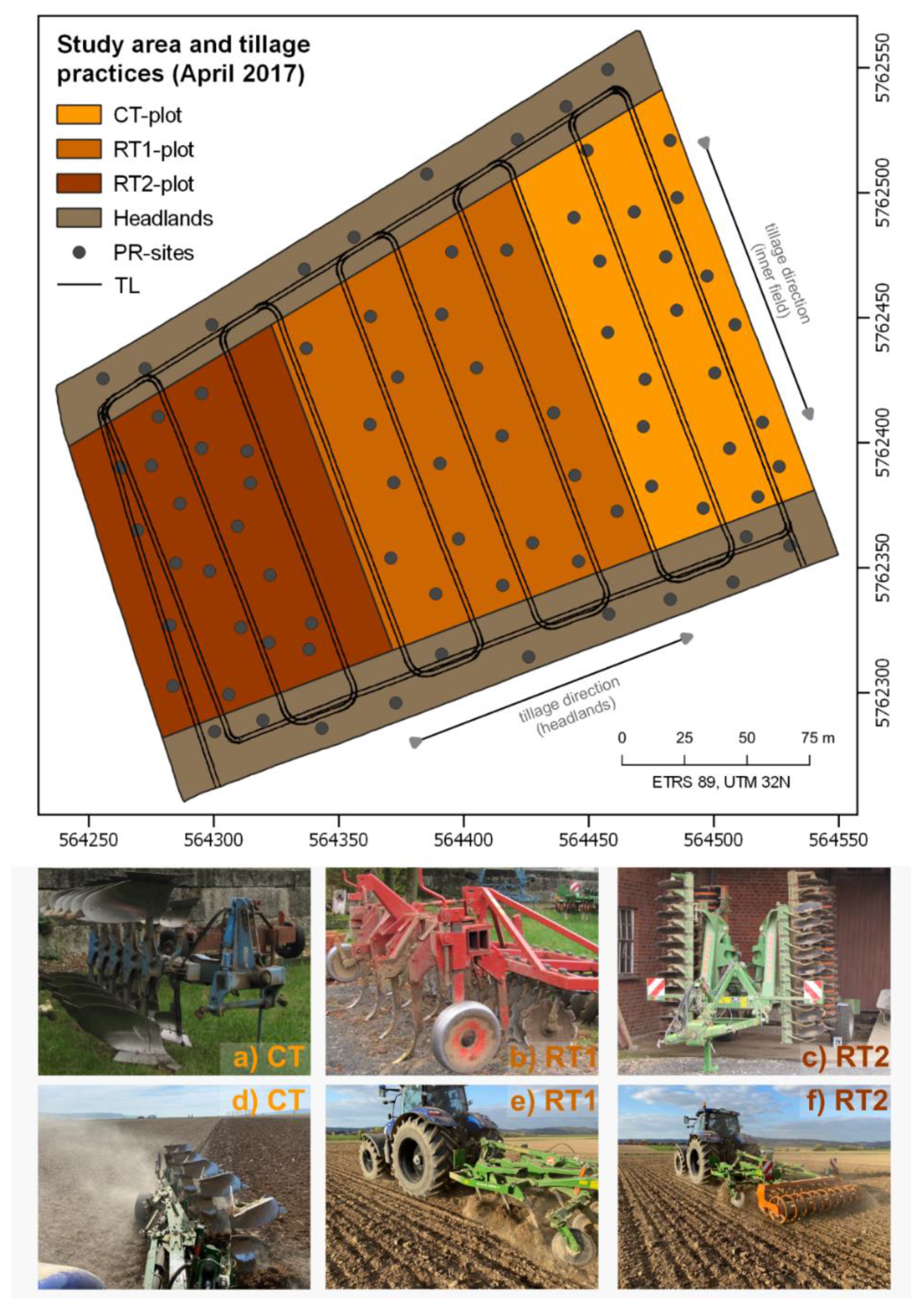
2.1. Study Area

The study area was located in Lower Saxony (Germany) and was one of the main study areas of the BonaRes-project “SOILAssist”. The field under study had a size of 5.5 ha and was separated into three areas with different tillage practices since 1996 (Figure 1).
The eastern part was conventionally tilled by moldboard plough to a depth of 30 cm (CT). In the central and western parts, reduced tillage with different degree of tillage intensity was established: (i) chisel plough to a depth of 25 cm (RT1) and (ii) disk harrow to a depth of 10 cm (RT2). According to Townsend et al. [47], RT1 can be classified as deep and RT2 as shallow reduced tillage.
After 18 years, the entire field was tilled with moldboard plough to a depth of 30 cm in October 2014, i.e., RT1 and RT2 were affected by OTIT. In the following year, the separation into the three tillage practices was re-established and conducted until now. For RT1, a composite tillage implement containing of a chisel and a harrow was used (Figure 1b,e). All three tillage implements (Figure 1a–c) were replaced by newer machinery types in October 2016 (Figure 1d–f), but without changing the tillage depth. All other field operations (e.g., sowing, fertilizing, harvest) were nearly identical for the three plots. Field traffic for spraying and fertilizing were conducted in tramlines (semi-permanent lanes) with a distance of 27 m. All other field traffic activities were random. A detailed description and analysis of all field traffic activities and the used machinery is given by Augustin et al. [50]. The headlands in the north and the south of the field were tilled with the chisel plough as used for the RT1 plot. The headland is the area of a field that has the highest field traffic intensity, since the turning maneuver of all field machinery occur in this area [50]. After harvest, all crop residues (straw, leaf of the beets, maize stubbles) were left on the field and were not removed.
The soil type of the study area was stagnic Luvisol [51] derived from deep weathered loess deposits. Soil texture is silt loam with 80% silt, 18% clay and 2% sand (average values). The fertile and high productive soil was in intensive agricultural use; typical crops were winter wheat (Triticum aestivum L.), sugar beets (Beta vulgaris L.) and maize (Zea mays L.). Crop rotation for the investigated period is given in Table 1. The climate is humid with mean annual precipitation of 741 mm and mean air temperature of 9.4 °C ([52], German Weather Service (DWD), weather station Hildesheim).

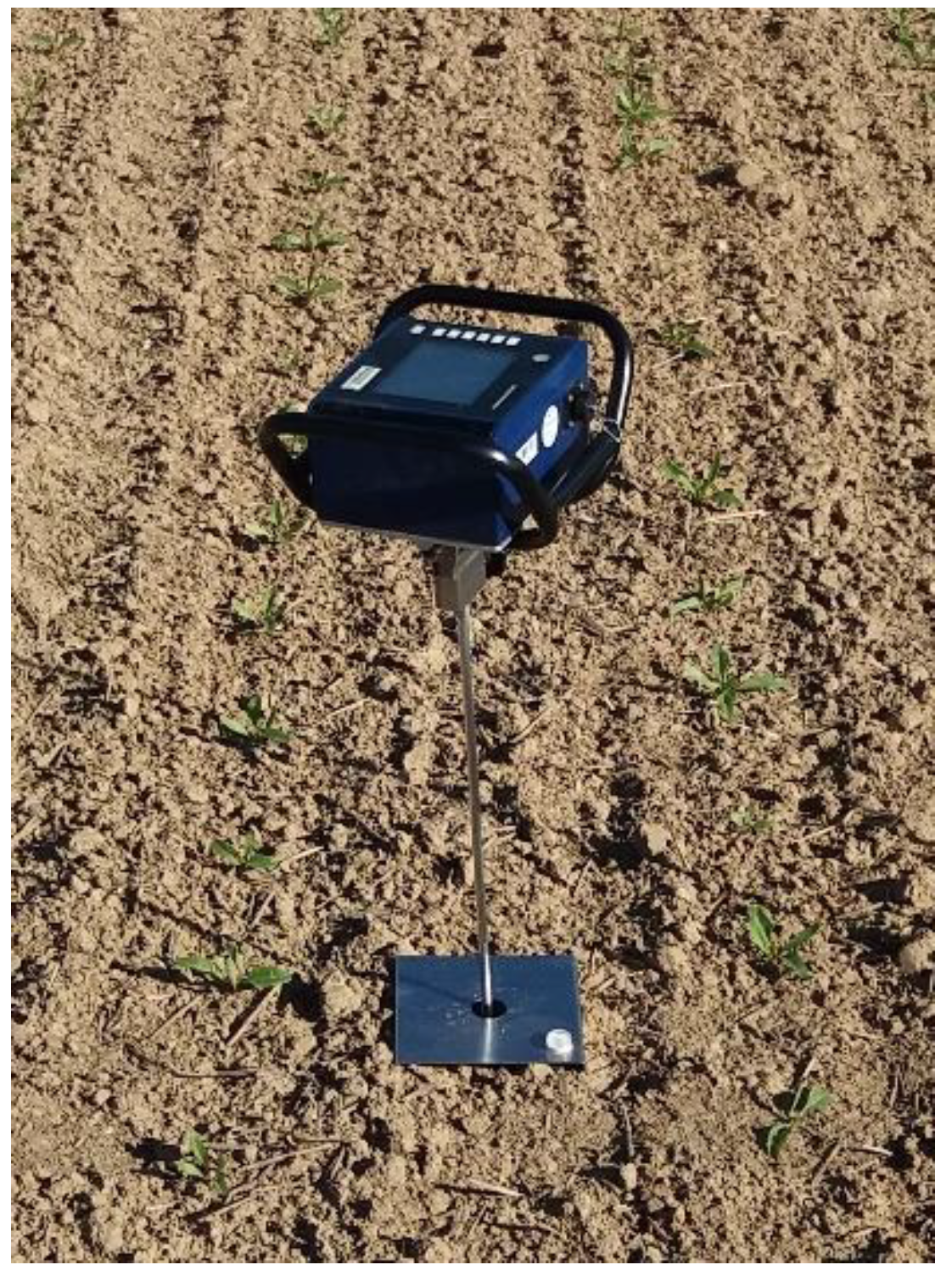
2.2. Measurement Design and Field Work

The fieldwork was carried out from 2014 to 2019 and focused on the measurement of the vertical penetration resistance of the soil. As short definition, penetration resistance gives the power (in MPa) which is necessary to press a defined cone into the soil (e.g., [53]). In June 2014, one measurement campaign was conducted before the OTIT. In the following year after OTIT, the penetration resistance was recorded three times (March, May and August 2015) to analyze the short-term effects. In the following years, one campaign per year was conducted to measure the penetration resistance (Table 1).
The locations for penetration resistance measurements were calculated using the stratified random point sampling method within the “Geospatial Modelling Environment” software (GME; version 0.7.2.1; [54]) connected to ArcGIS 10.1 (ESRI). Therefore, the field was divided into four subareas: CT, RT1, RT2 and the headlands. CT, RT1 and RT2 represented the three different tillage practices, while the headlands represented the area with the highest field traffic intensity [50,55]. For each subarea, a minimum of 15 points was calculated. Further boundary conditions for point selection were: (i) a minimum distance of 5 m between every generated point, (ii) a minimum distance of 5 m to known sampling points from earlier investigations, (iii) a minimum distance to the tramlines of 5 m and (iv) a minimum distance to field borders of 5 m. An identical procedure for point-calculation was used for the subsequent measurements. To avoid measurements at disturbed locations, all measured points from previous fieldwork got an additional distance-buffer of 5 m. Since the introduction of ArcGIS 10.3, GME was no longer supported. Therefore, we switched the random point calculation to QGIS. In this context, we changed the calculated points per area from 15 to 20 points to increase the point density for further analyses.
The randomly computed points were transferred to a handheld GPS (Juno SC, Trimble) which was used in the field to find the positions for the measurements. The penetration resistance was measured using a penetrologger (Penetrologger 06.15, Eijkelkamp; Figure 2) and a cone with a base area of 1 cm2 and an angle of 60°. The penetrologger was pressed into the soil by hand to a minimum depth of 45 cm at a mean velocity of 2 cm/s. The penetration resistance was automatically recorded in 1 cm depth intervals. As penetration resistance is highly variable, 5 parallel measurements were conducted at each point in a support size of 1 m2. In summary, between 300 and 400 measurements were performed during each field campaign, resulting in approximately 2500 measurements in total.
After penetration resistance measurements, all point positions were surveyed with a RTK-GPS (Viva CS 10, GNSS GS08plus, Leica) enabling an absolute accuracy of <20 cm.
In addition to the penetration resistance measurements, disturbed soil samples at 60 sites were collected with an auger (“Pürckhauer”) to analyze the soil texture and carbon content variations of the field. Both, soil texture and carbon content, are known to affect the soil penetration resistance [56,57,58]. Thus, their spatial distribution and variation must be considered for further analyses. The soil samples were collected at depth-intervals of 0–30 and 30–50 cm during the first investigation of the study area in March 2014 (Table 1). The point selection procedure for soil sampling was the same as for the determination of the locations for penetration resistance measurements.
As penetration resistance is sensitive to soil moisture [59,60], additional core samples were taken to determine the volumetric soil water content. Three to five sites in each tillage plot (CT, RT1 and RT2) were randomly selected to collect five core samples at each of this sites in a depth between 18 and 23 cm at all three dates in 2015, in May 2018 and in March 2019. The used core samples had a volume of 100 cm3 and a diameter of 6 cm. Further, the same core samples were used to determine the soil bulk density.

2.3. Laboratory Analyses

The disturbed soil samples were air-dried (35 °C), homogenized and sieved (<2 mm) for further analysis. The soil texture analyses were conducted by the sieve and pipette method according to Köhn [61]. Carbon content was determined with a C/N-Analyzer (EURO EA HEKAtech).
To determine the gravimetric soil water content and the bulk density, the core samples were weighed after soil sampling and subsequently dried at 105 °C for 24 h. Afterwards, the dried core samples were weighed again, and the volumetric soil water content was calculated [62,63].

2.4. Descriptive and Spatial Statistical Analyses

The statistical analyses were conducted with the software environment “R” [64]. For further analysis, the arithmetic means of the five replicate measurements of the penetration resistance per measuring site were calculated for each centimeter. Significant differences in means were tested using the Welch’s t-test.
Regionalization (also known as spatial interpolation) refers to methods used to map and analyze point observations in an area. Hamer et al. [65] provide an overview about the most common regionalization procedures. Since the regionalization of penetration resistance is based on the assumption that there is not a purely autocorrelative relationship in the spatial distribution of the target variable, but that other parameters influence this distribution, these other variables are initially regionalized. It is assumed that e.g., soil texture and carbon content exert a significant influence on penetration resistance [56]. Thus, both information, soil texture and carbon content, derived from the 60 sites of the field were used as spatial input variables for regionalization of penetration resistance. Regionalization of clay, silt and sand content for each soil layer (0–30 cm and 30–50 cm) was done using compositional kriging. Compositional kriging acknowledges the constant sum and non-negativity constraints of compositional data such as fractions of soil texture [66,67]. For carbon content, the ordinary kriging method was used [68,69]. For this purpose, automatically generated variograms were adapted to the point pairs and the values were regionalized by means of the autocorrelative behavior described in this way.
The tillage practices are assumed to have the strongest influence on the penetration resistance. However, since the procedures for the regionalization of the penetration resistance also include techniques that derive a regression between target variable and covariates, these categorical variables are converted using dummy coding [70].
To select the best fitting model to predict the spatial distribution of penetration resistance we compared the following regionalization methods using Leave-one-out cross-validations:
(i)
deterministic inverse distance weighting method (“gstat”, [71])
(ii)
geostatistical regionalization method ordinary kriging (“gstat”, [71]])
(iii)
machine learning methods multiple linear regression (“base R”, [64]), Regression Tree (“rpart”, [72]) and random forest (“randomForest” [73])
(iv)
procedures which combine geostatistical and machine learning methods such as kriging with external drift, regression tree kriging and random forest kriging (according to [65])
Two depth-intervals were selected to spatially predict penetration resistance: 16–25 cm and 36–45 cm. For regionalization, the arithmetic mean calculated from all penetration resistance values measured within these depth intervals were used. Based on the comparison of the prediction performance (cf. Table S1), the method with the lowest error for both depths and all years was selected for the final regionalization.
For the analyses of the volumetric soil water content and the bulk density, arithmetic means of the five core samples per measuring site were calculated.

3. Results

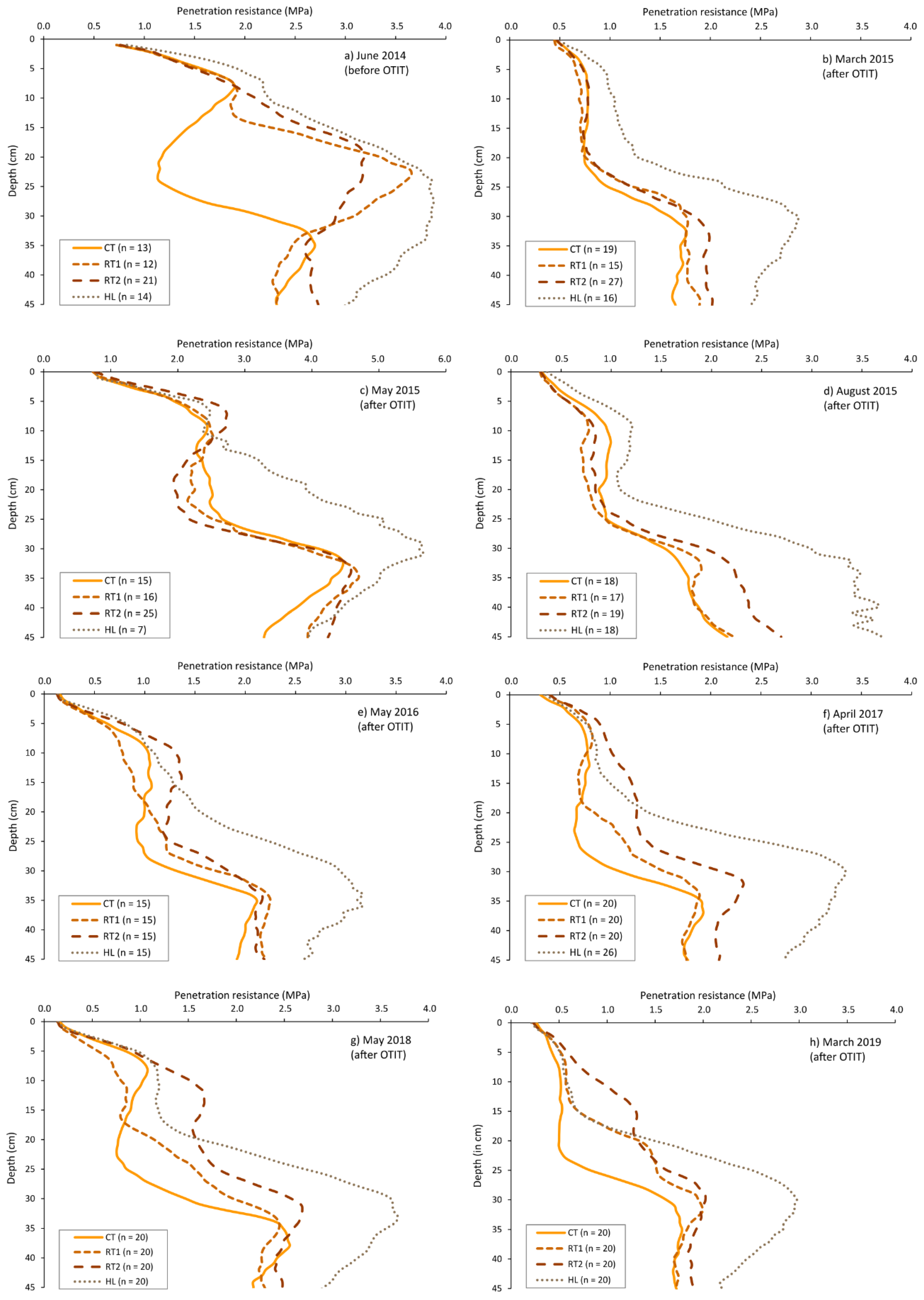
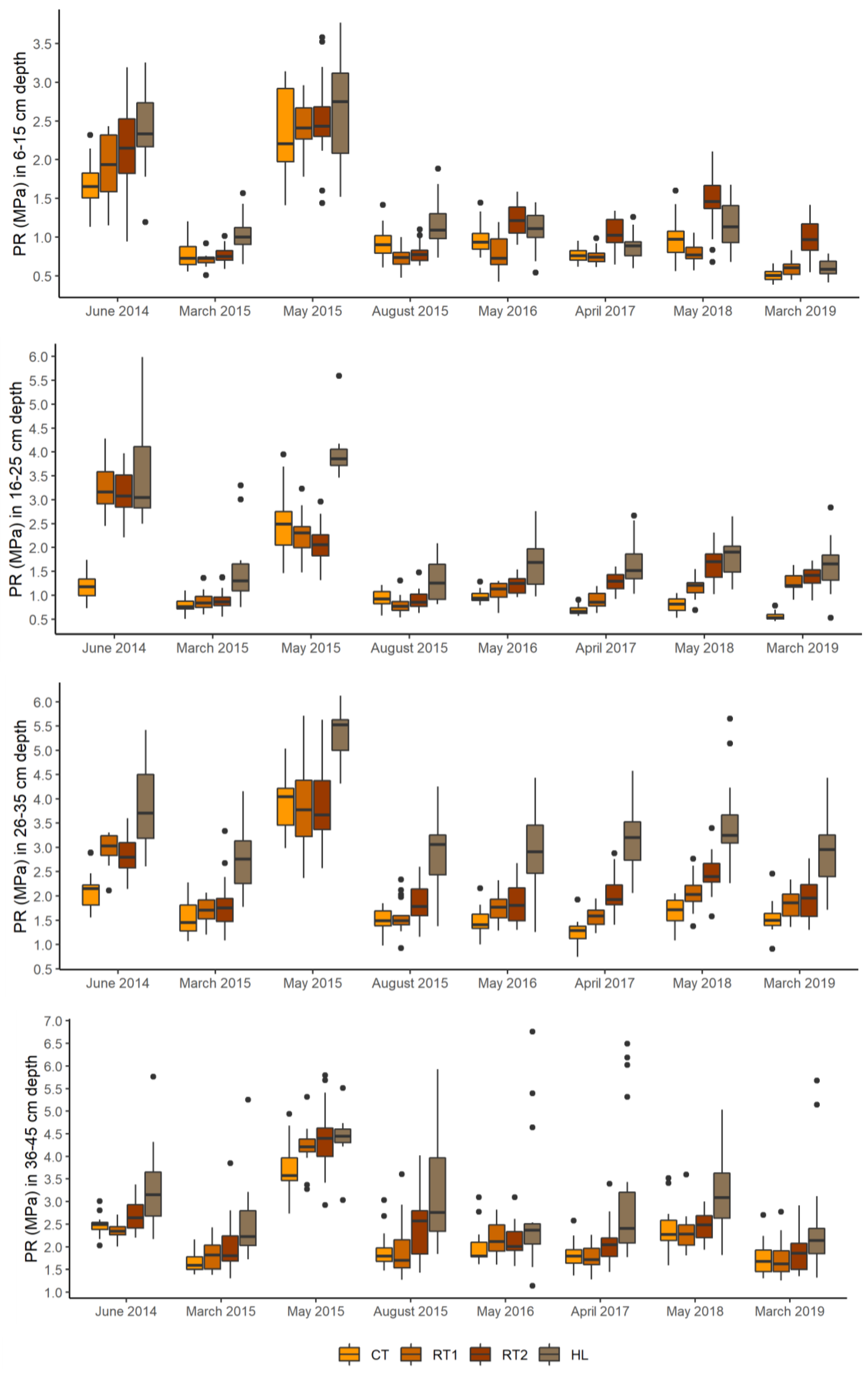
3.1. Penetration Resistance at Plot Scale

The depth profiles of the mean penetration resistance (Figure 3) and the associated box-whisker plots (Figure 4) were summarized in relation to the four field subsections (CT, RT1, RT2, HL). For each sampling point and date, the penetration resistance measurements of the individual subsections were averaged.
The penetration resistance recorded prior to OTIT in June 2014 revealed differences (p < 0.001) between CT and RT-plots (Figure 3a and Figure 4; Table 2). While penetration resistance increased to 1.8 MPa at a depth of 8 cm in all three treatments, penetration resistance strongly decreased to 1.1 MPa at a depth of about 25 cm in CT. In contrast, penetration resistance in both RT-plots continuously increased, reaching an averaged maximum of 3.2 MPa at a depth of 25 cm in RT2 and of 3.6 MPa at a depth of 22 cm in RT1. Below a depth of 33 cm the differences between the single tillage types disappear. Figure 3 further shows that penetration resistance was highest in the headlands, where a maximum of 3.9 MPa at a depth of 24 cm have been measured.
In 2015, the year after OTIT, the depth curves of RT1 and RT2 showed almost identical curve shapes as for CT (Figure 3b–d) and similar value distributions (Figure 4a–d). In March, May and August 2015, no differences between CT and the RT-plots occurred, except for three comparisons (Table 2). However, penetration resistance varied significantly (p < 0.01) within the season. In March penetration resistance was less than 1 MPa in all treatments to a depth of 20 cm. From 20 cm to 30 cm penetration resistance increased continuously to a maximum of 1.76 MPa (CT, RT1) and 1.95 MPa (RT2). The measurements revealed higher values in May. In the topmost 10 cm, penetration resistance increased continuously to 2.5 MPa. Although penetration resistance in CT remained nearly constant to a depth of 25 cm, it distinctly decreased in the RT-plots. Below 25 cm, the values increased steadily to the depths between 32 and 34 cm, reaching a maximum between 4.5–4.7 MPa in all treatments. In August, penetration resistance and the depth curves corresponded well to the measurements in March, with only slight differences between the single treatments.
In May 2016, the comparison between CT and RT1 further revealed no significant differences. In contrast, RT2 showed difference (p < 0.01) to CT in 6–15 and 16–25 cm and in 6–15 cm to RT1. One year later, in April 2017, all three plots differ significantly from each other in the topsoil (6–35 cm), except for CT-RT1 in 6–15 cm. The increase in penetration resistance in RT1 and RT2 is also apparent in Figure 3b and Figure 4b,c, where the distance between CT and RT1/2 respectively between RT1 and RT2 increased. The measurements in May 2018 revealed the same relationships as in April 2017, but with higher penetration resistance values in general. In March 2019, the comparison between CT and both RT-plots revealed the same differences as for 2018. In contrast to 2018, the differences between RT1 and RT2 are only significant for the depth 6–15 cm, but no longer for the soil layer beneath. In the subsoil layer (36–45 cm), no significant differences occurred between the three plots, except for May 2015 (CT-RT2).
Comparisons of penetration resistances between the interior sections and the headlands showed that measurements in the headlands were higher (p < 0.05) on all dates and nearly all depths (Figure 3 and Figure 4; Table 2).

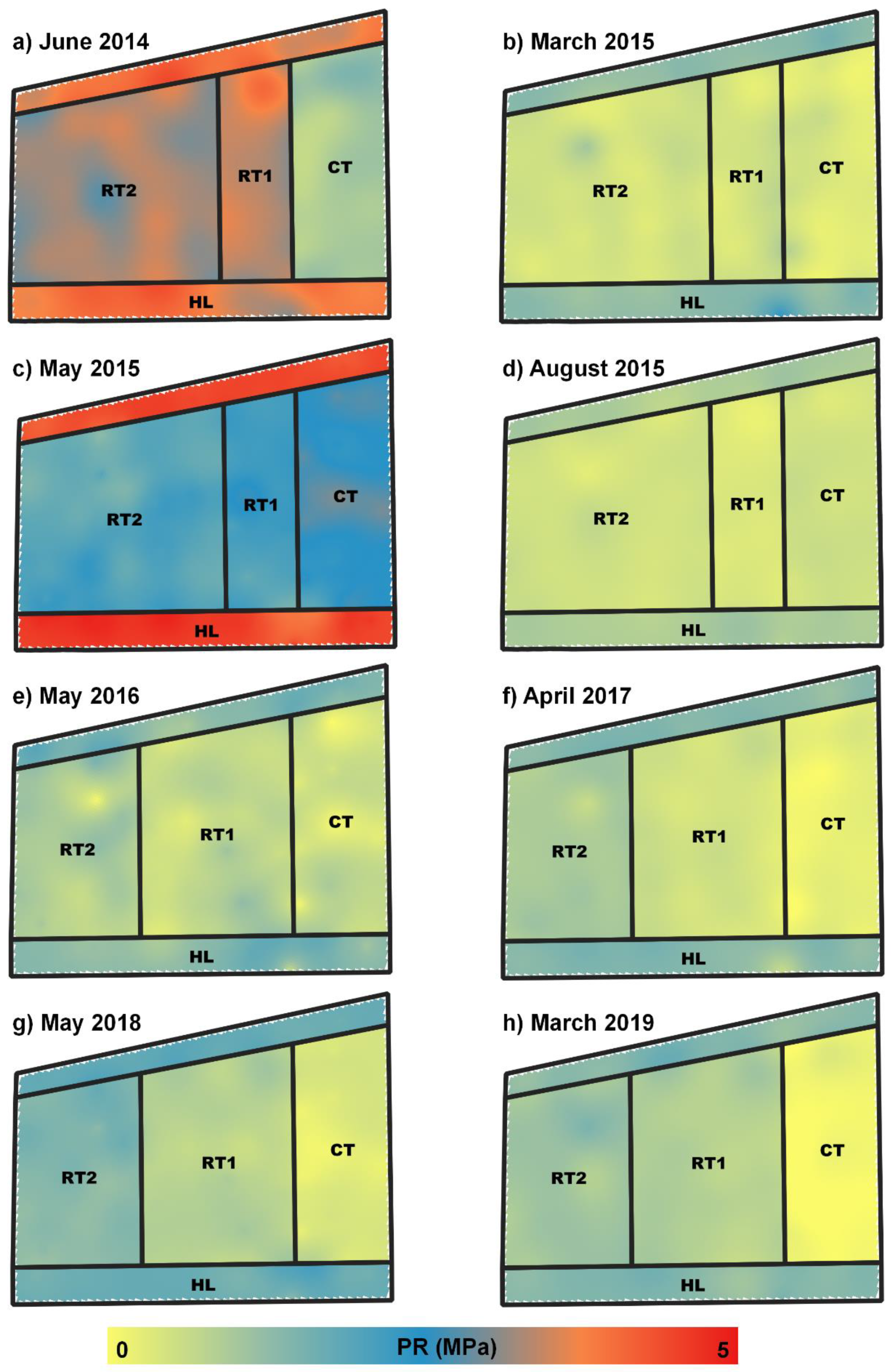
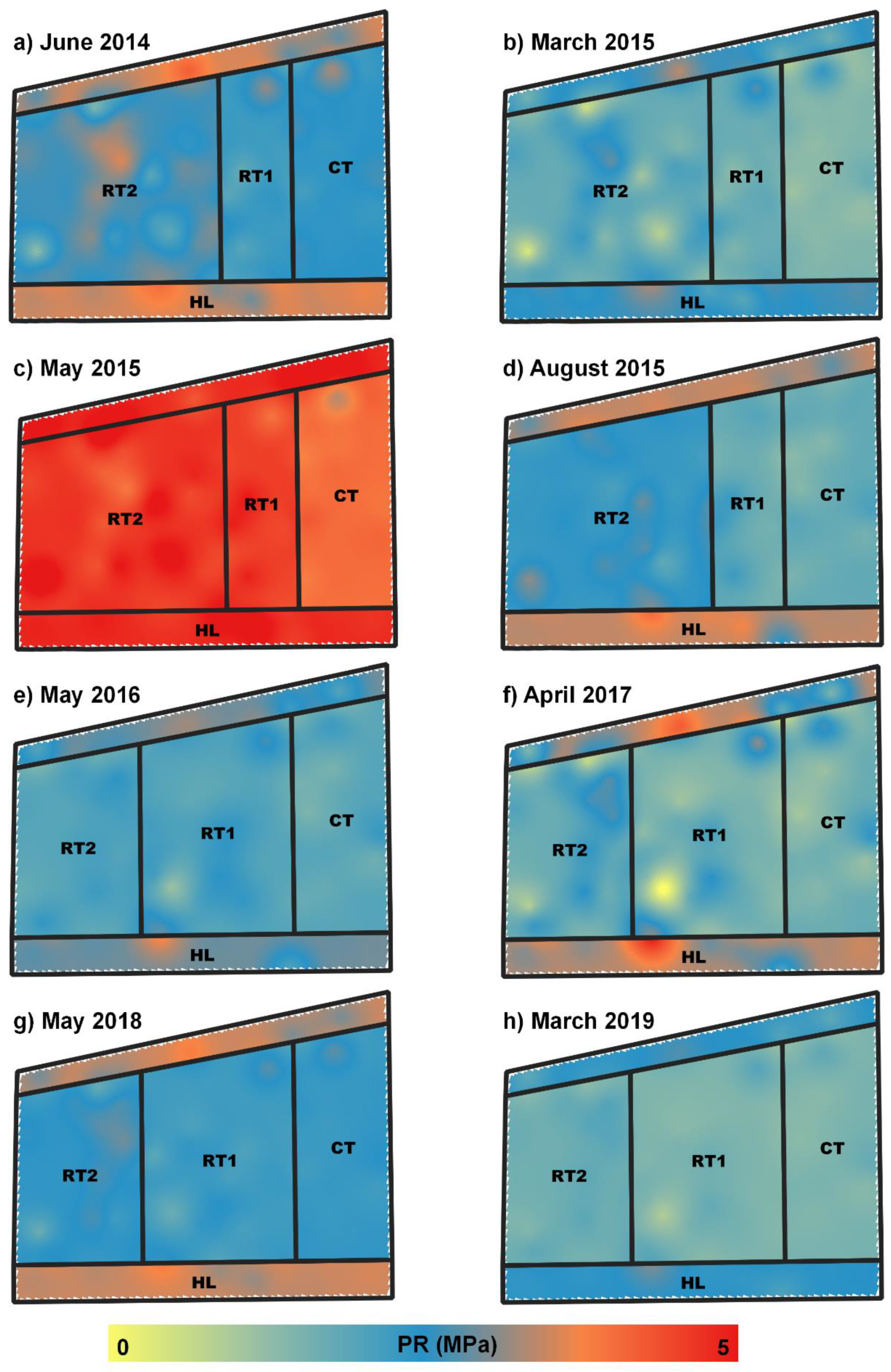
3.2. Spatial Patterns of Penetration Resistance

The errors of the regionalization procedures were determined through leave-one-out cross-validation. The residuals of each regionalization were then summarized using the mean absolute error (MAE) (Table S1). This error measure was chosen because isolated extreme values are typical for PR measurements. The commonly used root mean square error (RMSE) is associated with an overweighting of these outliers, while the MAE is less sensitive to the extremes.
The comparison (Table S1) showed that the single regionalization methods differ considerably, especially in 2014 and in May 2015, but only slightly over all years. None of the methods showed continuously the lowest error values. There was also no difference between pre-OTIT and post-OTIT. Most frequently, the predictions of the multiple linear regression (MLR) showed the lowest errors. In addition, the arithmetic mean for all years was the lowest error in the MLR procedure. Thus, the MLR procedure was chosen for the final regionalization (Figure 5 and Figure 6).
The MLR regionalization revealed differences in the spatial distribution of penetration resistance in the depth interval of 16–25 cm (Figure 5). Firstly, the inner field and the headlands could be spatially differentiated. On all dates, penetration resistance in the headlands was higher compared with those of the inner field. Although the values in the headlands varied widely over the season, the spatial pattern remained stable. Secondly, the three plots showed varying patterns among each other. Before OTIT, regionalized penetration resistance revealed clear differences between the three types of tillage (Figure 5a). The CT-plot showed lower values then both RT-plots. Directly after OTIT (Figure 5b–d), this subdivision in regionalization was no longer discernible. Since 2016, RT2 could be spatially distinguished from RT1 and CT (Figure 5e), followed by an increasing spatial differentiation between the three plots in the subsequent years (Figure 5f,g).
A similar trend could be seen in the importance of the covariates used for interpolation as shown by the absolute value of the t-statistic (Figure 7). The latter indicates the meaning of the individual co-variables on the prediction result. Before OTIT, only the soil parameters Ctot had an effect on the predicted penetration resistance values in soil depths between 16 and 25 cm. This effect is expressed by the slight variations of the interpolated penetration resistance inside the tillage practices (Figure 5a). These punctual influences of the interpolated total carbon content as well as the sand and clay contents—which themselves had no spatial tendency and only varied heterogeneously within small value range (cf. Section 3.3)—can be recognized in all predictions (Figure 5 and Figure 6). The tillage practices, particularly CT, determined the spatial forecast in 2014. After OTIT, the soil parameters gained increasing importance, although from 2017 onwards the importance of tillage practices increases again.
In the subsoil (36–45 cm), a clear spatial differentiation between the headlands and the three plots was identifiable for all dates (Figure 6). It also showed that penetration resistance strongly varies across the fields and throughout the years. In addition, nearly at each date single points with high respectively low penetration resistance within the field occurred. However, further differentiation of the three tillage plots as for the topsoil was not recognizable. This is also reflected in the t-statistic (Figure 7, 36–45 cm). Although tillage is usually more important than the other parameters, there was no change after 2014. On average, all values here had a lower importance (2.32) than the values of the depth between 16 and 25 cm (3.53).
For both depths, Figure 7 did not show a strong influence of the headland on the regionalization. In contrast to other machine learning methods, all covariates are always taken into account in Multiple Linear Regression. Since the dummy coding was used here, the values for moldboard plough, chisel plough and disk harrow were set to “0” if the headlands are set to “1”. But as this information is represented twice and led to the exclusion of a variable, the authors decided to delete the headland variable in order to be able to better compare the tillage methods.
For a similar reason, the silt was not considered as it showed a multicollinearity with clay and sand. The same applied to the sand content in the subsoil (36–45 cm). As it was also strongly correlated with the clay content in this depth, its influence is expressed by the clay content and is therefore not shown in Figure 7.

3.3. Soil Moisture, Bulk Density, Soil Texture and Carbon Content

The volumetric soil water content and the bulk density for the topsoil (18–23 cm depth) are shown in Table 3. The driest conditions were in May 2015 (around 25 vol.%), while in March 2015 the wettest conditions (35–39 vol.%) occurred. In the year after OTIT, CT had lightly higher volumetric soil water content compared to the RT-plots. In 2018 and 2019, the conditions reversed and both RT-plots had higher volumetric soil water contents, while RT2 showed the highest values. However, for all dates the variation of volumetric soil water content between the three plots was relatively low and not significant, except for March and August 2015.
The bulk density at the first measurement after OTIT in March 2015 revealed the lowest values in RT2 (1.38 g/cm3), followed by RT1 (1.40g/cm3) and CT (1.43 g/cm3). Two months later, in May 2015, all three plots exhibited the same bulk density (around 1.55 g/cm3). Thereafter, CT always revealed the lowest bulk density at each of the measuring dates, followed by RT1 and RT2.
No further soil samples were collected in 2016 and 2017, thus, no information about soil moisture or bulk density is available for that dates. The same is true for the soil properties before OTIT for this soil depth.
In the topsoil (0–30 cm), sand content was 3.2% (±1.0), silt content 78.9% (±2.0) and clay content 17.9% (±2.0). In the subsoil (30–50 cm), sand content was 2.8% (±1.0), silt content 77.9% (±2.6) and clay content 19.3% (±2.6). The carbon content was 1.22% (±0.17) in the topsoil and 0.72% (±0.17) in the subsoil.

4. Discussion

4.1. Temporal Effects of OTIT on Soil Penetration Resistance

The development of a compacted layer in the topsoil is typical in long-term reduced tillage as a result of soil settlement, soil compaction by field traffic and low loosening effects compared to conventional tillage [9,22,74]. These effects of long-term reduced tillage could be observed on the study area prior to OTIT. Compared to CT, both RT-plots showed higher values of penetration resistance in the topsoil (Figure 3a). A detailed description of the penetration resistance before OTIT is given by Kuhwald et al. [75].
The results of our study indicate that OTIT performed with a moldboard plough removed the compacted layer in the topsoil of both RT-plots. The former differences in penetration resistance between CT and both RT-plots (June 2014) were eliminated immediately after OTIT (2015). The same applies for the bulk density, which was in the same value range in all three plots after OTIT [32]. As expected [33,46], loosening and inversion by moldboard plough were able to remove the compacted layer in the topsoil and thus, one main aim of OTIT was reached. Thus, the three dates in 2015 showed no significant difference in penetration resistance in the topsoil. However, the variation between the dates was high, especially for May 2015 (Figure 4). The increase in pentation resistance in May 2015 was caused by low soil moisture (Table 3). With a water content of 25%, this date was the one with the lowest measured soil moisture. In August 2015, soil moisture increased again, resulting in a decrease of penetration resistance. This high sensitivity of penetration resistance to soil moisture is well known and frequently reported [56,60,76,77].
In May 2016, the first differences (p < 0.01) in penetration resistance between CT-RT2 and RT1-RT2 occurred. One year later, in April 2017, significant differences between CT and RT1 were observed. Two presumptions can be drawn from these results concerning the persistence effect of OTIT. The first one is that the enduring effect of OTIT on penetration resistance is relatively short. Already 18 months after OTIT, the re-development of a new compacted layer in RT2 had already started. From OTIT in October 2014 to the measurement in May 2016, field management throughout a complete winter wheat season (sowing, harvest; cf. Table 1) and over the first month of the silage maize season was carried out. All field traffic activities in this period are not related with very high soil compaction effects as is the case for silage maize or sugar beet harvest [19,78,79]. However, those field traffic activities were enough to re-establish a compacted layer in RT2 due to lower loosening effect by disk harrow.
The second presumption refers to the kind and depth of reduced tillage after OTIT. While significant differences in penetration resistance between CT and RT2 occurred after 19 months, it took 30 months until significant differences in penetration resistance between CT and RT1 developed. Reduced tillage with chisel plough is more intensive and deeper (25 cm) compared to disk harrow in RT2 (10 cm). Thus, the soil settlement and field traffic induced soil compaction effects in RT1 could be reduced to a greater extent, which led to a longer-lasting effect of OTIT on penetration resistance. However, differences between the three plots may have occurred earlier than the results indicate, because only one measurement per year was conducted since August 2015. For instance, it could be assumed that penetration resistance reached higher values already after silage maize harvest in autumn 2016. On our study area, silage maize harvest was carried out with heavy load machinery having wheel loads of about 7 Mg. In addition, the amount of wheel passage was high [50]. Both can increase the soil compaction and, therefore, also the penetration resistance [19,80]. Thus, the enduring effect of OTIT in RT1 might be reduced to 24 months.
Final penetration resistance measurements in March 2019 revealed further change between RT1 and RT2. In contrast to the previous two years, where RT1 and RT2 showed significant differences in penetration resistance at almost all depths, these differences disappeared. This holds especially true for the depth intervals from 16 to 25 cm and from 26 to 35 cm, indicating that the penetration resistance of both RT-treatments is approaching each other over time (Figure 3h). In autumn 2018, the sugar beet harvest was conducted with a self-propelled harvester which exhibited a maximum wheel load of 10 Mg and wheeled nearly 100% of the entire field [50]. Thus, the soil compaction risk especially in the topsoil was extremely high, although soil moisture was relatively low due to low precipitation (cf. Figure S1) during harvest. As a result, the penetration resistance between the two RT plots approximate. Thus, for our study area after one complete crop rotation, the state of penetration resistance corresponds approximately to the state observed before OTIT.

4.2. Spatial Effects of OTIT on Penetration Resistance

Figure 4 illustrates that the denser layer formed during long-term reduced tillage had been removed through one-time moldboard ploughing. OTIT led to a homogenization of the penetration resistances across the entire field, especially under moist soil conditions in March and August (Figure 5). Before OTIT in 2014 (Figure 5a), CT and RT can be clearly spatially distinguished. In 2015 (Figure 5b–d), after OTIT, the regionalization showed only slight differences between the three types of tillage. From 2016 onward, a difference between the plots becomes apparent.
The analysis of the various regionalization approaches has shown that there are only minimal differences between the methods insofar as no procedure consistently achieve the best results (Table S1). The fact that a model solely based on covariates, such as MLR, produces lower errors than geostatistical methods using Kriging (Table S1), leads to the conclusion that the spatial autocorrelation of the target variable provides much less information about the spatial distribution than the covariates. This implies that the tillage practice has a considerably stronger influence than the soil parameters used (Figure 7). Its effect is much more pronounced in the topsoil, suggesting that the penetration resistance is strongly influenced by tillage, especially in the soil depths directly changed by tillage.
Another influence on penetration resistance can be seen in the higher values in the regionalization (Figure 5a,c) and the higher MAE (Table S1) in June 2014 and May 2015. Before OTIT in June 2014, the long-term conservation tillage led to increased penetration resistance in both RT-plots [75]. In May 2015, the soil moisture was considerably lower (Table 3) compared to the other measuring dates, which led to higher penetration resistance values. These higher penetration resistance values led to the increased MAE.
The changes in penetration resistance are much less pronounced in the depth of 36–45 cm (Figure 6). The tillage practice is consistently less important here (Figure 7). The soil parameters are much more important relative to the tillage practice than at shallower depths. Thus, the influence of tillage practice on the penetration resistance in the subsoil is lower. Consequently, OTIT had no effect on subsoil penetration resistance. However, the headlands can be clearly distinguished from the inner field as a result of the intensive field traffic in this area [50].

4.3. Assessment, Advances and Limitations of Penetration Resistance Measurements

The previous chapters discussed the temporal and spatial aspects of penetration resistance before and after OTIT. A question that remains is: how to assess the penetration resistance values in terms of evaluating the effects of soil compaction after OTIT? One assessment may be based on the time, when significant differences between CT and RT occurred again. After 18 (RT2) and 30 (RT1) months, the positive effects of OTIT on penetration resistance were no longer measurable (cf. Section 4.1). Another assessment can be made by using the absolute values of penetration resistance. In literature, penetration resistance between 2 and 3 MPa, measured at field capacity, are assumed as upper limit values for root growth [81,82,83]. Exceeding these values may result in restricted root growth and lower plant biomass and yield. In contrast, Peixoto et al. [36] recommended the measurement of penetration resistance at lower soil moisture when the aim is to evaluate soil compaction. Based on laboratory measurements, they recommend measurement at 0.1 MPa (pF 3.0) instead of field capacity (around pF 1.8). For our study area, volumetric soil water content at field capacity (pF 1.8) is at 37% (±0.02). Related to pF 3.0, as recommended by Peixoto et al. [36], volumetric water content equals 28% (±0.03). Before OTIT, both RT-plots and the headlands revealed penetration resistance values greater than 2 MPa in the top- and subsoil (cf. Figure 3 and Figure 4). However, as no soil moisture information is available for the topsoil, an assignment to a pF-value is not feasible. However, at a depth of 30–35 cm, volumetric soil water content was at 32 vol.% and thus between pF 1.8 and 3.0 [75]. After OTIT, the measurements from March 2015 were conducted at soil moisture near field capacity, while measurements in May 2015 were conducted at pF > 3.0. All other measurements were between pF 1.8 and 3.0. The critical value of 2 MPa was reached in the topsoil (16–25 cm) only in May 2015, while measurements at the other dates were below 2 MPa. Only from a depth of 25 cm downward, values greater than 2 MPa occurred occasionally.
However, as long as no clear threshold value of penetration resistance for restricted root growths exists, an assessment based an absolute values is critical. This is one of the limitations in the use of penetration resistance for assessment purposes. In general, penetration resistance is often used in literature to evaluate the status of soil compaction (e.g., [84,85]). Some studies showed that there is a positive correlation between penetration resistance and bulk density [58,86], while others found contrary results [87]. These contrary results may be attributed to the high sensitivity of penetration resistance to soil moisture.
However, increased penetration resistance and bulk density do not necessarily indicate harmful soil compaction. Many soils under conservation tillage can exhibit higher penetration resistance but at the same time increased saturated hydraulic conductivity, infiltration rate or air permeability [9,75,87]. Thus, it must be kept in mind that penetration resistance alone may not able to give information about soil functionality like hydraulic conductivity or yield effects [33,75]. Furthermore, penetration resistance is highly sensitive to soil moisture state [56,60]. For comparisons, similar soil water contents are required. While measurements at field capacity are recommended to ensure comparability [53], measurement of penetration resistance at drier conditions may be necessary to assess soil compaction [36]. For the investigated field, soil moisture variation in the topsoil within the field was relatively low (cf. Table 3). However, variation in soil moisture during the investigated period showed clearly the effects of varying soil moisture states on the absolute values of penetration resistance. Thus, the greater the differences within a field (e.g., due to geomorphology or parent material variation), the greater the differences in penetration resistance, which may hamper a meaningful evaluation. Moreover, other soil formation processes such as cementation by oxides may result in increased penetration resistance [88]. However, as a fast and minimal-invasive measurement, penetration resistance has proven as a good indicator for a first evaluation of soil compaction states [89].

5. Conclusions

This study showed that OTIT can remove the compacted layer that has developed in long-term reduced tillage as indicated by penetration resistance measurements. Moreover, the spatio-temporal analyses of the following 5 years showed a relatively fast re-increase in penetration resistance in the reduced tilled plots (18 respectively 30 months). Thus, the positive effects of OTIT on soil compaction may noticeably short.
This study was conducted on high productive silty soils which are under intensive agricultural use. Especially the crops maize and sugar beets are related with high soil compaction risk. A change of crop rotation to crops with less soil compaction risk (e.g., rapeseed, oat) may extend the time until penetration resistance increases again. Further, the effects on clay or sandy soils may be different and must be part of future studies. In addition, the effect of OTIT on penetration resistance may last longer when the soil is affected by several freeze-thaw cycles in winter. However, the study area was not affected by intense freeze-thaw cycles during the investigated period due to relatively warm winters.
In summary, OTIT is one option to lower soil compaction in long-term conservation tillage. To prolong its positive effects, the field traffic impact after OTIT should be as low as possible, e.g., by reducing wheel loads and wheel pass frequencies or by choosing crops with low soil compaction risk. Additionally, an overall assessment of OTIT necessitates consideration of further topics such as energy consumption, effects on soil carbon content and effects on soil erosion.

Supplementary Materials

The following are available online at https://www.mdpi.com/2073-445X/9/12/482/s1.

Author Contributions

M.K. designed the study in collaboration with all co-authors. M.K. and W.B.H. conducted the data analyses, prepared the tables and figures and wrote the majority of the text. J.B. and R.D. contributed in reviewing and finalizing the manuscript. All authors have read and agreed to the published version of the manuscript.

Funding

The Federal Ministry of Education and Research (BMBF) supported this study within the framework of the BonaRes-initiative (Grant No.: 031B0684C). We acknowledge financial support for publications cost by Land Schleswig-Holstein within the funding programme Open Access Publikationsfonds.

Acknowledgments

We are grateful to A. Berger, J. Goldmann and M. Gosse for assistance in the laboratory. Furthermore, we thank C. Thomas, K. Augustin and F. Behrens for fieldwork support. The authors thank the anonymous reviewers for their commitment and very helpful comments on improving the manuscript.

Conflicts of Interest

The authors declare no conflict of interest.

References

  1. Pittelkow, C.M.; Liang, X.; Linquist, B.A.; Van Groenigen, K.J.; Lee, J.; Lundy, M.E.; Van Gestel, N.; Six, J.; Venterea, R.T.; Van Kessel, C. Productivity limits and potentials of the principles of conservation agriculture. Nature 2015, 517, 365–368. [Google Scholar] [CrossRef]
  2. Kassam, A.; Friedrich, T.; Derpsch, R. Global spread of Conservation Agriculture. Int. J. Environ. Stud. 2018, 76, 29–51. [Google Scholar] [CrossRef]
  3. Prestele, R.; Hirsch, A.L.; Davin, E.L.; Seneviratne, S.I.; Verburg, P.H. A spatially explicit representation of conservation agriculture for application in global change studies. Glob. Chang. Biol. 2018, 24, 4038–4053. [Google Scholar] [CrossRef] [PubMed]
  4. Busari, M.A.; Kukal, S.S.; Kaur, A.; Bhatt, R.; Dulazi, A.A. Conservation tillage impacts on soil, crop and the environment. Int. Soil Water Conserv. Res. 2015, 3, 119–129. [Google Scholar] [CrossRef] [Green Version]
  5. Sanaullah, M.; Usman, M.; Wakeel, A.; Cheema, S.A.; Ashraf, I.; Farooq, M. Terrestrial ecosystem functioning affected by agricultural management systems: A review. Soil Tillage Res. 2020, 196, 104464. [Google Scholar] [CrossRef]
  6. FAO. Conservation Agriculture—Revised Version; AG Dept Factsheets: Rome, Italy, 2017. [Google Scholar]
  7. Luo, Z.; Wang, E.; Sun, O.J. Soil carbon change and its responses to agricultural practices in Australian agro-ecosystems: A review and synthesis. Geoderma 2010, 155, 211–223. [Google Scholar] [CrossRef]
  8. Li, Y.; Chang, S.X.; Tian, L.; Zhang, Q. Conservation agriculture practices increase soil microbial biomass carbon and nitrogen in agricultural soils: A global meta-analysis. Soil Biol. Biochem. 2018, 121, 50–58. [Google Scholar] [CrossRef]
  9. Horn, R. Time Dependence of Soil Mechanical Properties and Pore Functions for Arable Soils. Soil Sci. Soc. Am. J. 2004, 68, 1131–1137. [Google Scholar] [CrossRef]
  10. Tebrügge, F.; Düring, R.-A. Reducing tillage intensity—A review of results from a long-term study in Germany. Soil Tillage Res. 1999, 53, 15–28. [Google Scholar] [CrossRef]
  11. Lal, R.; Reicosky, D.C.; Hanson, J.D. Evolution of the plow over 10,000 years and the rationale for no-till farming. Soil Tillage Res. 2007, 93, 1–12. [Google Scholar] [CrossRef]
  12. Lal, R. Restoring Soil Quality to Mitigate Soil Degradation. Sustainability 2015, 7, 5875–5895. [Google Scholar] [CrossRef] [Green Version]
  13. Nail, E.L.; Young, D.L.; Schillinger, W.F. Diesel and glyphosate price changes benefit the economics of conservation tillage versus traditional tillage. Soil Tillage Res. 2007, 94, 321–327. [Google Scholar] [CrossRef]
  14. Lahmar, R. Adoption of conservation agriculture in Europe: Lessons of the KASSA project. Land Use Policy 2010, 27, 4–10. [Google Scholar] [CrossRef]
  15. Lou, Y.; Xu, M.; Chen, X.; He, X.; Zhao, K. Stratification of soil organic C, N and C:N ratio as affected by conservation tillage in two maize fields of China. CATENA 2012, 95, 124–130. [Google Scholar] [CrossRef]
  16. Deubel, A.; Hofmann, B.; Orzessek, D. Long-term effects of tillage on stratification and plant availability of phosphate and potassium in a loess chernozem. Soil Tillage Res. 2011, 117, 85–92. [Google Scholar] [CrossRef]
  17. Bajwa, A.A. Sustainable weed management in conservation agriculture. Crop Prot. 2014, 65, 105–113. [Google Scholar] [CrossRef]
  18. Nichols, V.; Verhulst, N.; Cox, R.; Govaerts, B. Weed dynamics and conservation agriculture principles: A review. Field Crops Res. 2015, 183, 56–68. [Google Scholar] [CrossRef] [Green Version]
  19. Destain, M.-F.; Roisin, C.; Dalcq, A.-S.; Mercatoris, B.C.N. Effect of wheel traffic on the physical properties of a Luvisol. Geoderma 2016, 262, 276–284. [Google Scholar] [CrossRef]
  20. Blanco-Canqui, H.; Ruis, S.J. No-tillage and soil physical environment. Geoderma 2018, 326, 164–200. [Google Scholar] [CrossRef]
  21. Nunes, M.R.; Denardin, J.E.; Pauletto, E.A.; Faganello, A.; Pinto, L.F.S. Mitigation of clayey soil compaction managed under no-tillage. Soil Tillage Res. 2015, 148, 119–126. [Google Scholar] [CrossRef] [Green Version]
  22. Bogunovic, I.; Pereira, P.; Kisic, I.; Sajko, K.; Sraka, M. Tillage management impacts on soil compaction, erosion and crop yield in Stagnosols (Croatia). CATENA 2018, 160, 376–384. [Google Scholar] [CrossRef]
  23. D’Haene, K.; Vermang, J.; Cornelis, W.M.; Leroy, B.L.M.; Schiettecatte, W.; de Neve, S.; Gabriels, D.; Hofman, G. Reduced tillage effects on physical properties of silt loam soils growing root crops. Soil Tillage Res. 2008, 99, 279–290. [Google Scholar] [CrossRef]
  24. Daraghmeh, O.A.; Jensen, J.R.; Petersen, C.T. Soil structure stability under conventional and reduced tillage in a sandy loam. Geoderma 2009, 150, 64–71. [Google Scholar] [CrossRef]
  25. Vogeler, I.; Horn, R.; Wetzel, H.; Krümmelbein, J. Tillage effects on soil strength and solute transport. Soil Tillage Res. 2006, 88, 193–204. [Google Scholar] [CrossRef]
  26. Dang, Y.P.; Seymour, N.P.; Walker, S.R.; Bell, M.J.; Freebairn, D.M. Strategic tillage in no-till farming systems in Australia’s northern grains-growing regions: I. Drivers and implementation. Soil Tillage Res. 2015, 152, 104–114. [Google Scholar] [CrossRef]
  27. Dang, Y.P.; Moody, P.W.; Bell, M.J.; Seymour, N.P.; Dalal, R.C.; Freebairn, D.M.; Walker, S.R. Strategic tillage in no-till farming systems in Australia’s northern grains-growing regions: II. Implications for agronomy, soil and environment. Soil Tillage Res. 2015, 152, 115–123. [Google Scholar] [CrossRef]
  28. Dang, Y.P.; Balzer, A.; Crawford, M.; Rincon-Florez, V.; Liu, H.; Melland, A.R.; Antille, D.; Kodur, S.; Bell, M.J.; Whish, J.P.M.; et al. Strategic tillage in conservation agricultural systems of north-eastern Australia: Why, where, when and how? Environ. Sci. Pollut. Res. Int. 2018, 25, 1000–1015. [Google Scholar] [CrossRef]
  29. Baan, C.D.; Grevers, M.C.J.; Schoenau, J.J. Effects of a single cycle of tillage on long-term no-till prairie soils. Can. J. Soil Sci. 2009, 89, 521–530. [Google Scholar] [CrossRef]
  30. Crawford, M.H.; Rincon-Florez, V.; Balzer, A.; Dang, Y.P.; Carvalhais, L.C.; Liu, H.; Schenk, P.M. Changes in the soil quality attributes of continuous no-till farming systems following a strategic tillage. Soil Res. 2015, 53, 263–273. [Google Scholar] [CrossRef]
  31. Quincke, J.A.; Wortmann, C.S.; Mamo, M.; Franti, T.; Drijber, R.A.; García, J.P. One-Time Tillage of No-Till Systems. Agron. J. 2007, 99, 1104–1110. [Google Scholar] [CrossRef]
  32. Kuhwald, M.; Blaschek, M.; Brunotte, J.; Duttmann, R. Comparing soil physical properties from continuous conventional tillage with long-term reduced tillage affected by one-time inversion. Soil Use Manag. 2017, 33, 611–619. [Google Scholar] [CrossRef]
  33. Çelik, İ.; Günal, H.; Acar, M.; Acir, N.; Bereket Barut, Z.; Budak, M. Strategic tillage may sustain the benefits of long-term no-till in a Vertisol under Mediterranean climate. Soil Tillage Res. 2019, 185, 17–28. [Google Scholar] [CrossRef]
  34. Blanco-Canqui, H.; Wortmann, C.S. Does occasional tillage undo the ecosystem services gained with no-till: A review. Soil Tillage Res. 2020, 198, 104534. [Google Scholar] [CrossRef]
  35. Peixoto, D.S.; Silva, L.d.C.M.d.; Melo, L.B.B.d.; Azevedo, R.P.; Araújo, B.C.L.; Carvalho, T.S.d.; Moreira, S.G.; Curi, N.; Silva, B.M. Occasional tillage in no-tillage systems: A global meta-analysis. Sci. Total Environ. 2020, 745, 140887. [Google Scholar] [CrossRef] [PubMed]
  36. Peixoto, D.S.; Silva, B.M.; Oliveira, G.C.d.; Moreira, S.G.; da Silva, F.; Curi, N. A soil compaction diagnosis method for occasional tillage recommendation under continuous no tillage system in Brazil. Soil Tillage Res. 2019, 194, 104307. [Google Scholar] [CrossRef]
  37. Crawford, M.H.; Bell, K.; Kodur, S.; Dang, Y.P. The Influence of Tillage Frequency on Crop Productivity in Sub-Tropical to Semi-Arid Climates. J. Crop Sci. Biotechnol. 2018, 21, 13–22. [Google Scholar] [CrossRef]
  38. Liu, H.; Crawford, M.; Carvalhais, L.C.; Dang, Y.P.; Dennis, P.G.; Schenk, P.M. Strategic tillage on a Grey Vertosol after fifteen years of no-till management had no short-term impact on soil properties and agronomic productivity. Geoderma 2016, 267, 146–155. [Google Scholar] [CrossRef]
  39. Kettler, T.A.; Lyon, D.J.; Doran, J.W.; Powers, W.L.; Stroup, W.W. Soil Quality Assessment after Weed-Control Tillage in a No-Till Wheat–Fallow Cropping System. Soil Sci. Soc. Am. J. 2000, 64, 339–346. [Google Scholar] [CrossRef] [Green Version]
  40. Baker, D.B.; Johnson, L.T.; Confesor, R.B.; Crumrine, J.P. Vertical Stratification of Soil Phosphorus as a Concern for Dissolved Phosphorus Runoff in the Lake Erie Basin. J. Environ. Qual. 2017, 46, 1287–1295. [Google Scholar] [CrossRef] [Green Version]
  41. Melland, A.R.; Antille, D.L.; Dang, Y.P. Effects of strategic tillage on short-term erosion, nutrient loss in runoff and greenhouse gas emissions. Soil Res. 2017, 55, 201. [Google Scholar] [CrossRef]
  42. Smith, D.R.; Warnemuende, E.A.; Huang, C.; Heathman, G.C. How does the first year tilling a long-term no-tillage field impact soluble nutrient losses in runoff? Soil Tillage Res. 2007, 95, 11–18. [Google Scholar] [CrossRef]
  43. Chauhan, B.S.; Singh, R.G.; Mahajan, G. Ecology and management of weeds under conservation agriculture: A review. Crop Prot. 2012, 38, 57–65. [Google Scholar] [CrossRef]
  44. Renton, M.; Flower, K.C. Occasional mouldboard ploughing slows evolution of resistance and reduces long-term weed populations in no-till systems. Agric. Syst. 2015, 139, 66–75. [Google Scholar] [CrossRef]
  45. Nunes, M.R.; Pauletto, E.A.; Denardin, J.E.; Suzuki, L.E.A.S.; van Es, H.M. Dynamic changes in compressive properties and crop response after chisel tillage in a highly weathered soil. Soil Tillage Res. 2019, 186, 183–190. [Google Scholar] [CrossRef]
  46. Leao, T.P.; da Silva, A.P.; Tormena, C.A.; Giarola, N.F.; Figueiredo, G.C. Assessing the immediate and residual effects of chiseling for ameliorating soil compaction under long-term no-tillage. J. Soil Water Conserv. 2014, 69, 431–438. [Google Scholar] [CrossRef]
  47. Townsend, T.J.; Ramsden, S.J.; Wilson, P. How do we cultivate in England? Tillage practices in crop production systems. Soil Use Manag. 2016, 32, 106–117. [Google Scholar] [CrossRef] [Green Version]
  48. Salem, H.M.; Valero, C.; Muñoz, M.Á.; Rodríguez, M.G.; Silva, L.L. Short-term effects of four tillage practices on soil physical properties, soil water potential, and maize yield. Geoderma 2015, 237–238, 60–70. [Google Scholar] [CrossRef] [Green Version]
  49. Alvarez, R.; Steinbach, H.S. A review of the effects of tillage systems on some soil physical properties, water content, nitrate availability and crops yield in the Argentine Pampas. Soil Tillage Res. 2009, 104, 1–15. [Google Scholar] [CrossRef]
  50. Augustin, K.; Kuhwald, M.; Brunotte, J.; Duttmann, R. Wheel Load and Wheel Pass Frequency as Indicators for Soil Compaction Risk: A Four-Year Analysis of Traffic Intensity at Field Scale. Geosciences 2020, 10, 292. [Google Scholar] [CrossRef]
  51. FAO. World reference base for soil resources. International soil classification system for naming soils and creating legends for soil maps. In World Soil Resources Report 106; FAO: Rome, Italy, 2014. [Google Scholar]
  52. DWD. Climate Data Center (CDC). Available online: https://cdc.dwd.de/portal/ (accessed on 21 August 2020).
  53. Arriaga, F.J.; Lowery, B.; Raper, R. Soil Penetrometers and Penetrability. In Encyclopedia of Agrophysics; Gliński, J., Horabik, J., Lipiec, J., Eds.; Springer Netherlands: Dordrecht, The Netherlands, 2011; pp. 757–760. ISBN 978-90-481-3585-1. [Google Scholar]
  54. Beyer, H.L. Geospatial Modelling Environment (Version 0.7.2.1). Available online: http://www.spatialecology.com/gme/ (accessed on 3 March 2014).
  55. Duttmann, R.; Brunotte, J.; Bach, M. Spatial analyses of field traffic intensity and modeling of changes in wheel load and ground contact pressure in individual fields during a silage maize harvest. Soil Tillage Res. 2013, 126, 100–111. [Google Scholar] [CrossRef]
  56. Kumar, A.; Chen, Y.; Sadek, A.; Rahman, S. Soil cone index in relation to soil texture, moisture content, and bulk density for no-tillage and conventional tillage. Agric. Eng. Int. CIGR J. 2012, 14, 26–37. [Google Scholar]
  57. Dexter, A.R.; Czyż, E.A.; Gaţe, O.P. A method for prediction of soil penetration resistance. Soil Tillage Res. 2007, 93, 412–419. [Google Scholar] [CrossRef]
  58. Kılıç, K.; Özgöz, E.; Akbaş, F. Assessment of spatial variability in penetration resistance as related to some soil physical properties of two fluvents in Turkey. Soil Tillage Res. 2004, 76, 1–11. [Google Scholar] [CrossRef]
  59. Vaz, C.M.P.; Manieri, J.M.; de Maria, I.C.; Tuller, M. Modeling and correction of soil penetration resistance for varying soil water content. Geoderma 2011, 166, 92–101. [Google Scholar] [CrossRef]
  60. Vaz, C.M.P.; Bassoi, L.H.; Hopmans, J.W. Contribution of water content and bulk density to field soil penetration resistance as measured by a combined cone penetrometer–TDR probe. Soil Tillage Res. 2001, 60, 35–42. [Google Scholar] [CrossRef] [Green Version]
  61. Gee, G.W.; Bauder, J.W. Particle-size Analysis. In Methods of Soil Analysis: Part 1; Soil Science Society of America; American Society of Agronomy: Madison, WI, USA, 1986; pp. 383–411. [Google Scholar]
  62. Blake, G.R.; Hartge, K.H. Bulk density. In Methods of Soil Analysis: Part 1; Soil Science Society of America; American Society of Agronomy: Madison, WI, USA, 1986; pp. 363–375. [Google Scholar]
  63. Gardner, W.H. Water Content. In Methods of Soil Analysis: Part 1; Soil Science Society of America; American Society of Agronomy: Madison, WI, USA, 1986; pp. 493–544. [Google Scholar]
  64. R Core Team. R: A Language and Environment for Statistical Computing; R Foundation for Statistical Computing: Vienna, Austria, 2020. [Google Scholar]
  65. Hamer, W.B.; Birr, T.; Verreet, J.-A.; Duttmann, R.; Klink, H. Spatio-Temporal Prediction of the Epidemic Spread of Dangerous Pathogens Using Machine Learning Methods. IJGI 2020, 9, 44. [Google Scholar] [CrossRef] [Green Version]
  66. De Gruijter, J.J.; Walvoort, D.J.J.; van Gams, P.F.M. Continuous soil maps—A fuzzy set approach to bridge the gap between aggregation levels of process and distribution models. Geoderma 1997, 77, 169–195. [Google Scholar] [CrossRef]
  67. Walvoort, D.J.J.; De Gruijter, J.J. Compositional Kriging: A Spatial Interpolation Method for Compositional Data. Math. Geol. 2001, 33, 951–966. [Google Scholar] [CrossRef]
  68. Yao, X.; Yu, K.; Deng, Y.; Liu, J.; Lai, Z. Spatial variability of soil organic carbon and total nitrogen in the hilly red soil region of Southern China. J. For. Res. 2019, 210, 455. [Google Scholar] [CrossRef] [Green Version]
  69. Hu, C.; Li, F.; Xie, Y.H.; Deng, Z.M.; Hou, Z.Y.; Li, X. Spatial distribution and stoichiometry of soil carbon, nitrogen and phosphorus along an elevation gradient in a wetland in China. Eur. J. Soil Sci. 2019. [Google Scholar] [CrossRef]
  70. Erjavec, N. Dummy Variables. International Encyclopedia of Statistical Science; Springer: Berlin/Heidelberg, Germany, 2011; pp. 407–408. [Google Scholar]
  71. Pebesma, E.J. Multivariable geostatistics in S: The gstat package. Comput. Geosci. 2004, 30, 683–691. [Google Scholar] [CrossRef]
  72. Therneau, T.; Atkinson, B. Rpart: Recursive Partitioning and Regression Trees. R Package Version 4.1-15. Available online: https://github.com/bethatkinson/rpart (accessed on 10 August 2020).
  73. Liaw, A.; Wiener, M. Classification and Regression by randomForest. R. News 2002, 2, 18–22. [Google Scholar]
  74. Jirků, V.; Kodešová, R.; Nikodem, A.; Mühlhanselová, M.; Žigová, A. Temporal variability of structure and hydraulic properties of topsoil of three soil types. Geoderma 2013, 204–205, 43–58. [Google Scholar] [CrossRef]
  75. Kuhwald, M.; Blaschek, M.; Minkler, R.; Nazemtseva, Y.; Schwanebeck, M.; Winter, J.; Duttmann, R. Spatial analysis of long-term effects of different tillage practices based on penetration resistance. Soil Use Manag. 2016, 32, 240–249. [Google Scholar] [CrossRef]
  76. Whalley, W.R.; To, J.; Kay, B.D.; Whitmore, A.P. Prediction of the penetrometer resistance of soils with models with few parameters. Geoderma 2007, 137, 370–377. [Google Scholar] [CrossRef]
  77. Gao, W.; Watts, C.W.; Ren, T.; Whalley, W.R. The effects of compaction and soil drying on penetrometer resistance. Soil Tillage Res. 2012, 125, 14–22. [Google Scholar] [CrossRef]
  78. Peth, S.; Horn, R.; Fazekas, O.; Richards, B.G. Heavy soil loading its consequence for soil structure, strength, deformation of arable soils. J. Plant Nutr. Soil Sci. 2006, 169, 775–783. [Google Scholar] [CrossRef]
  79. Kuhwald, M.; Dörnhöfer, K.; Oppelt, N.; Duttmann, R. Spatially Explicit Soil Compaction Risk Assessment of Arable Soils at Regional Scale: The SaSCiA-Model. Sustainability 2018, 10, 1618. [Google Scholar] [CrossRef] [Green Version]
  80. Koch, H.-J.; Dieckmann, J.; Büchse, A.; Märländer, B. Yield decrease in sugar beet caused by reduced tillage and direct drilling. Eur. J. Agron. 2009, 30, 101–109. [Google Scholar] [CrossRef]
  81. Pardo, A.; Amato, M.; Chiarandà, F.Q. Relationships between soil structure, root distribution and water uptake of chickpea (Cicer arietinum L.). Plant growth and water distribution. Eur. J. Agron. 2000, 13, 39–45. [Google Scholar] [CrossRef]
  82. Otto, R.; Silva, A.P.; Franco, H.C.J.; Oliveira, E.C.A.; Trivelin, P.C.O. High soil penetration resistance reduces sugarcane root system development. Soil Tillage Res. 2011, 117, 201–210. [Google Scholar] [CrossRef]
  83. Bengough, A.G.; McKenzie, B.M.; Hallett, P.D.; Valentine, T.A. Root elongation, water stress, and mechanical impedance: A review of limiting stresses and beneficial root tip traits. J. Exp. Bot. 2011, 62, 59–68. [Google Scholar] [CrossRef] [PubMed] [Green Version]
  84. Botta, G.F.; Tolon-Becerra, A.; Lastra-Bravo, X.; Tourn, M. Tillage and traffic effects (planters and tractors) on soil compaction and soybean (Glycine max L.) yields in Argentinean pampas. Soil Tillage Res. 2010, 110, 167–174. [Google Scholar] [CrossRef]
  85. Braunack, M.V.; Johnston, D.B. Changes in soil cone resistance due to cotton picker traffic during harvest on Australian cotton soils. Soil Tillage Res. 2014, 140, 29–39. [Google Scholar] [CrossRef]
  86. Barik, K.; Aksakal, E.L.; Islam, K.R.; Sari, S.; Angin, I. Spatial variability in soil compaction properties associated with field traffic operations. CATENA 2014, 120, 122–133. [Google Scholar] [CrossRef]
  87. Gozubuyuk, Z.; Sahin, U.; Ozturk, I.; Celik, A.; Adiguzel, M.C. Tillage effects on certain physical and hydraulic properties of a loamy soil under a crop rotation in a semi-arid region with a cool climate. CATENA 2014, 118, 195–205. [Google Scholar] [CrossRef]
  88. Bayat, H.; Kolahchi, Z.; Valaey, S.; Rastgou, M.; Mahdavi, S. Iron and magnesium nano-oxide effects on some physical and mechanical properties of a loamy Hypocalcic Cambisol. Geoderma 2019, 335, 57–68. [Google Scholar] [CrossRef]
  89. Peixoto, D.S.; Silva, B.M.; Godinho Silva, S.H.; Karlen, D.L.; Moreira, S.G.; Pereira da Silva, A.A.; Vilela de Resende, Á.; Norton, L.D.; Curi, N. Diagnosing, Ameliorating, and Monitoring Soil Compaction in No-Till Brazilian Soils. Agrosyst. Geosci. Environ. 2019, 2, 1–14. [Google Scholar] [CrossRef] [Green Version]
Figure 1. Study area with the plots separated by different tillage practices and the headlands (April 2017). CT: continuously conventional tilled plot; RT1: reduced tilled plot (chisel plough), affected by one-time inversion tillage; RT2 reduced tilled plot (disc harrow), affected by one-time inversion tillage; PR-sites: Sites of penetration resistance measurements. TL: Tramlines. Photographs (ac) show the tillage implements of 2014 and 2015, photographs (df) the tillage implements for 2016–2019.
Land 09 00482 g001
Figure 2. Photograph of the used penetrologger.
Land 09 00482 g002
Figure 3. Penetration resistance profiles from 0 to 45 cm depth in 1 cm intervals. For each sampling date (ah), the penetration resistance measurements were averaged for the three former tillage practices (CT: continuously conventional tilled plot, both reduced tilled plots affected by one-time inversion tillage (RT1: chisel plough; RT2: disc harrow). Records in the headlands (HL) were separated from those of the inner field and displayed on an individual graph.
Land 09 00482 g003
Figure 4. Box-whisker plots of penetration resistance (PR) comparing continuously conventional tilled plot (CT), both reduced tilled plots affected by one-time inversion tillage (RT1: chisel plough; RT2: disc harrow) and the headlands (HL) at 6–15 cm, 16–25 cm, 26–35 cm, and 36–45 cm.
Land 09 00482 g004
Figure 5. Predicted penetration resistance (PR) in the depth of 16–25 cm using Multiple Linear Regression (MLR). Conventional tilled plot (CT), both reduced tilled plots affected by one-time inversion tillage (RT1: chisel plough; RT2: disc harrow) and the headlands (HL).
Land 09 00482 g005
Figure 6. Predicted penetration resistance (PR) in the depth of 36–45 cm using Multiple Linear Regression (MLR). Conventional tilled plot (CT), both reduced tilled plots affected by one-time inversion tillage (RT1: chisel plough; RT2: disc harrow) and the headlands (HL).
Land 09 00482 g006
Figure 7. Importance of the variables expressed by the absolute value of the t-statistic for each parameter of the MLR models used to interpolate the penetration resistance (Figure 5 and Figure 6; CT: continuously conventional tilled plot, both reduced tilled plots affected by one-time inversion tillage (RT1: chisel plough; RT2: disc harrow); Ctot: total carbon).
Land 09 00482 g007
Table 1. Crop rotation, important field activities and dates of field work.
YearField CropPrimary TillageSowingHarvestFieldwork
2014Sugar beets20–21 March 201423 April 20148 and 16 October 201410–14 March a and 11–13 June b 2014
2014/15Winter wheat18 October 201418 October 201413 August 201523–27 March bc, 26–29 May bc, 19–21 August bc 2015
2016Maize21 and 22 April 201623 April 201627 September 20169–11 May b 2016
2016/17Winter wheat4 October 20164 October 20169 August 201710–11 April b 2017
2018Sugar beets8 and 9 April 201810 April 201825 October 20186–9 May bc 2018
2018/19Winter wheat26 October 201826 October 201830 July 201925–29 March bc 2019
a: collection of disturbed soil samples, b: measurement of penetration resistance, c: collection of undisturbed soil samples. A detailed description of all used machinery and all field traffic activities is given by Agustin et al. [50].
Table 2. Significance of differences in mean penetration resistance comparing conventional tillage, reduced tillage practices and the headlands, subdivided into 10-cm depth intervals.
Depth in cm Depth in cm
6–1516–2526–3536–45 6–1516–2526–3536–45
June 2014 aCT-RT1n.s.******n.s.May 2016 bCT-RT1n.s.n.s.n.s.n.s.
CT-RT2n.s.******n.s.CT-RT2*****n.s.n.s.
RT1-RT2n.s.n.s.n.s.** RT1-RT2***n.s.n.s.n.s.
HL-IF********** HL-IFn.s.********
March 2015 bCT-RT1n.s.n.s.n.s.n.s.April 2017 bCT-RT1n.s.******n.s.
CT-RT2n.s.n.s.n.s.n.s.CT-RT2*********n.s.
RT1-RT2n.s.n.s.n.s.n.s. RT1-RT2*********n.s.
HL-IF************ HL-IFn.s.*********
May 2015 bCT-RT1n.s.n.s.n.s.n.s.May 2018 bCT-RT1********n.s.
CT-RT2n.s.n.s.n.s.**CT-RT2*********n.s.
RT1-RT2n.s.n.s.n.s.n.s. RT1-RT2********n.s.
HL-IFn.s.******n.s. HL-IFn.s.*********
August 2015 bCT-RT1**n.s.n.s.n.s.March 2019 bCT-RT1*******n.s.
CT-RT2n.s.n.s.**n.s.CT-RT2********n.s.
RT1-RT2n.s.n.s.n.s.n.s. RT1-RT2***n.s.n.s.n.s.
HL-IF************ HL-IFn.s.*********
n.s.: not significant; ** significant at p < 0.01; *** significant at p < 0.001; a: before one-time inversion tillage; b: after one-time inversion tillage; CT: continuously conventional tilled plot; RT1: reduced tilled plot (chisel plough), affected by one-time inversion tillage; RT2 reduced tilled plot (disc harrow), affected by one-time inversion tillage.
Table 3. Comparison of volumetric soil water content and bulk density after OTIT in a depth between 18 and 23 cm.
March 2015May 2015August 2015May 2018March 2019
Tillage PlotVSWC
%
BD
g/cm3
VSWC
%
BD
g/cm3
VSWC
%
BD
g/cm3
VSWC
%
BD
g/cm3
VSWC
%
BD
g/cm3
CT38.5
(±1.1) a
1.43
(±0.03) a
25.2
(±0.3) a
1.55
(±0.03) a
36.0
(±0.6) a
1.44
(±0.01) a
29.3
(±2.2) a
1.27
(±0.06) a
31.7
(±0.6) a
1.31
(±0.02) a
RT135.8
(±2.2) ab
1.40
(±0.04) a
24.9
(±2.0) a
1.55
(±0.05) a
34.9
(±0.4) b
1.45
(±0.03) a
32.1
(±2.2) a
1.36
(±0.06) b
31.8
(±1.1) a
1.39
(±0.03) b
RT234.6
(±1.9) bc
1.38
(±0.06) a
24.5
(±4.1) a
1.54
(±0.09) a
33.8
(±1.2) b
1.46
(±0.02) a
33.4
(±0.9) a
1.46
(±0.03) c
31.9
(±1.0) a
1.45
(±0.03) c
VSWC = volumetric soil water content; BD = bulk density; (±) = standard deviation; CT: continuously conventional tilled plot; RT1: reduced tilled plot (chisel plough), affected by one-time inversion tillage; RT2 reduced tilled plot (disc harrow), affected by one-time inversion tillage; same letters indicate no significant differences at p < 0.05 (two-sample t-test) within the three tillage plots for the single soil physical properties. Values from 2015 first published by Kuhwald et al. [30].
Publisher’s Note: MDPI stays neutral with regard to jurisdictional claims in published maps and institutional affiliations.

