Forest Area Change in the Shifting Landscape Mosaic of the Continental United States from 2001 to 2016

Abstract

The landscape context (i.e., anthropogenic setting) of forest change partly determines the social-ecological outcomes of the change. Furthermore, forest change occurs within, is constrained by, and contributes to a dynamic landscape context. We illustrate how information about local landscape context can be incorporated into regional assessments of forest area change. We examined the status and change of forest area in the continental United States from 2001 to 2016, quantifying landscape context by using a landscape mosaic classification that describes the dominance and interface (i.e., juxtaposition) of developed and agriculture land in relation to forest and other land. The mosaic class changed for five percent of total land area and three percent of total forest area. The least stable classes were those comprising the developed interface. Forest loss rates were highest in developed-dominated landscapes, but the forest area in those landscapes increased by 18 percent as the expansion of developed landscapes assimilated more forest area than was lost from earlier developed landscapes. Conversely, forest loss rates were lowest in agriculture-dominated landscapes where there was a net loss of five percent of forest area, even as the area of those landscapes also increased. Exposure of all land to nearby forest removal, fire, and stress was highest in natural-dominated landscapes, while exposure to nearby increases in developed and agriculture land was highest in developed- and agriculture-dominated landscapes. We discuss applications of our approach for mapping, monitoring, and modeling landscape and land use change.

1. Highlights

The landscape context changed for 5.3 percent of the area of the continental United States. The landscape context was least stable in the interfaces between developed and undeveloped land.

The percent of forest area exhibiting a change of landscape context (3.2 percent) was larger than the net percent loss of forest area (2.6 percent).

Forest loss rates were highest in developed landscapes but there was a 17.7 percent increase of forest area in those landscapes because they expanded into forested areas.

Conversely, forest loss rates were lowest in agricultural landscapes but there was a 4.7 percent decrease of forest area in those landscapes, even as the area of those landscapes also increased.

The landscape context of forest change provides new evidence that most forest loss was temporary and was the result of pervasive forestry operations.

2. Introduction

The importance of forest and landscape changes are well-documented in the ecology and land use literature. To support natural resource management and strategic forest planning pursuant to the United States Resources Planning Act (RPA; P.L. 93-378, 88 Stat 475, as amended), the objective of this study was to examine forest change in the continental United States (CONUS) from 2001 to 2016 in relation to the dynamic landscape context within which the forest changes occurred. Forest change is common throughout the forests of North America. Much of the evidence of recent forest change comes from temporal analyses of satellite images, primarily by evaluating vegetation indices in terms of stand-clearing events. Masek et al. [1] reported a loss of 0.9% of forest area per year from 1990 to 2000, with local rates approaching 3% per year. Hansen et al. [2] estimated the mean annual forest loss from 2000 to 2005 was ~50,000 km² per year, which is equivalent to an annual loss of ~0.9%. In the CONUS, Schleeweis et al. [3] found that similar rates of forest disturbance were sustained over a longer time period during 1986–2020. While climate change likely plays a role in forest loss [4], pervasive forestry operations appear to be the primary driver of forest change over most of the CONUS, with secondary drivers (e.g., insects, diseases, fire) affecting an increasing area of forest over time [1,3,5,6]. Forest loss due to land use conversion from forest to agriculture or urban land persists longer than other forest area changes, and although such conversions are smaller in total area, they are also pervasive and locally important where they occur [6,7].

Despite the evidence of large forest losses, the total CONUS “forestland” area (i.e., the area that is “used” as forest) has been stable for several decades [8,9]. These seemingly disparate findings are reconciled by Coulston et al. [10], who noted that forest land use does not imply continuous forest cover, and that net change of forest cover also depends on forest cover gain which balances forest cover loss. Supporting both perspectives are CONUS land cover data from 2001 to 2016 which show that the large area of forest cover loss approximated the area gained, and that most of the transitions from (or to) forest cover were typically to (or from) shrub and grass forest cover [7]. Those types of transitions are consistent with the attribution of forest loss to forestry operations because grass and shrub covers are transitional, early-succession land covers that accompany natural or artificial forest regeneration [9].

Both net and gross forest area changes have additional shortcomings as indicators of forest change because they ignore not only the spatial pattern of change but also the landscape context (or “setting”) within which the change occurs. The fact that forest is both lost and gained during a specified interval implies that the spatial distribution of the forest cover must change over that interval, even if net forest area remains the same. The spatial patterns of forest change are not necessarily uniform with respect to landscape context, and the rate of change varies substantially among different types of landscapes even as the landscapes themselves change over time [11]. Especially important is the appearance or expansion of intensive land uses such as agriculture and infrastructure (e.g., buildings, roads) near forest areas, which sets up new ecological risks, societal concerns, and management challenges for forests. That is so because the landscape context partly determines the specific effects of a forest change, including the value that society places on that event, and it constrains forest management options and efficacy. For example, a wildfire in a suburban area has a very different set of ecological and social-economic consequences when compared to a fire in a wilderness area, and in both settings fire management options are constrained by the transportation infrastructure, and restoration efficacy depends on what type of forest is restored [12]. Similarly, invasive species management must consider landscape context because nearby intensive land uses increase forest invasibility, introduce exotic species, and constrain management options [13,14,15,16]. Local forest managers have long considered landscape context, as evidenced by forested stream buffers [17], visual screens along roadways [18], and the location of forest-based recreation experiences [19]. There is now a need for regional assessments to also consider the geography of forest change, as it relates to the evolving landscape context within which the change occurs.

A notable example in the United States is the recent focus on the “wildland-urban interface” which arose in response to concerns about water quality and wildfire [20]. From a broader perspective, however, the expansion of the wildland-urban interface is only a part of the total picture of landscape change. Urban expansion also encroaches upon adjacent agricultural landscapes which contain forest, and in agriculture-urban interfaces the forest may be valued mainly for its rarity. In contrast, the dynamics of forest within agricultural settings depend primarily on the relative economic benefit of tree crops versus other crops [21] and incentives such as the Conservation Reserve Program [22]. An even broader perspective recognizes the goal of “keeping forests as forest” [23] which implies maintenance of forest-dominated landscapes even as expanding agriculture and urban land uses compete with forest land use and form interface areas within those landscapes. Put simply, forest cannot be sustained unless forested landscapes are sustained [11]. Even casual observation shows that continued expansion of an urban (or agriculture) interface within a forested landscape leads to a landscape that is dominated by developed (or agricultural) land and that the remnant forest exists within a novel landscape context. From a systems theoretic perspective, such changes in landscape “dominance” have social-ecological implications that are more fundamental than those arising in landscape “interfaces” [24].

Qualitative concepts like landscape context and setting have been quantified for regional forest assessments [25,26]. This study was designed to improve the 2020 CONUS RPA assessment by extending landscape analyses to consider forest area dynamics in relation to landscape change over time. We characterized overall landscape change and then refined the analysis to examine forest change within the changing landscapes. Our conceptual model has three parts to consider land cover change, exposure to nearby change processes, and the landscape context of the exposure and change. Both conceptually and in practice, changes to and from forest cover occur at specific locations, such that transition matrices prepared from land cover maps provide an appropriate model for analyses. We implemented analyses of forest cover change using the National Land Cover Database (NLCD) [7]. We also conceptualized the exposure of a given location to a nearby change in terms of the edge effects of that change, which typically permeates the immediate neighborhood of the change [27,28]. We evaluated five types of exposures in the neighborhood of each location. Three types of forest change (forest removal, forest fire, and forest stress) were identified using the North American Forest Dynamics–Attribution (NAFD-ATT) disturbance attribution map [3], and two types of land use change (increased agriculture or developed cover) were identified from the NLCD land cover maps. More than one change process can (and often does) occur in the same neighborhood, for example where forest removal is followed by increased developed cover. For simplicity, we ignored interactions among change processes and analyzed each process type separately. The conceptual model of landscape context emphasizes the importance of intensive human land uses (i.e., agriculture and development), which have been the primary drivers of global forest area change for centuries [29]. We implemented that concept by using the landscape mosaic classification [30], which is an indicator of overall ecological condition [31] that also quantifies landscape dominance and interfaces [32]. Each location was described by the proportions of agriculture and developed land covers in relation to all other land cover within a surrounding neighborhood. For consistency with forest cover change data, we implemented the landscape mosaic classification using the same NLCD land cover data.

The first objective of our investigation was to examine overall changes in the landscape mosaic, dominance, and interface in the continental United States from 2001 to 2016. The second objective was to characterize the exposure to change processes that occurred within each landscape mosaic from 2001 to 2010, and to evaluate how much of each mosaic class area was exposed to those processes. Our third objective was to examine forest change in relation to changes of the landscape context including to the landscape mosaic, dominance, and interface from 2001 to 2016. We discuss the results in terms of evidence supporting whether forest change was temporary versus permanent, and natural versus anthropogenic, and we suggest applications of our approach for mapping, monitoring, and modeling landscape and land use change.

3. Materials and Methods

3.1. Synopsis

We implemented our conceptual models in a raster framework by classifying each 0.09-ha location (a 30 m by 30 m pixel) in the continental United States according to: its landscape mosaic class as determined in the surrounding 65.61-ha (27 pixels by 27 pixels) neighborhood in 2001 and 2016, and thus according to its landscape dominance and landscape interface classes which are aggregations of the mosaic classes; the forest cover status (forest, nonforest) at that location in 2001 and 2016, and; the evidence (yes or no) of exposure to five types of change processes within the surrounding 4.41-ha (7 pixels by 7 pixels) neighborhood from 2001 to 2010. The landscape mosaic naturally changes with the size of the neighborhood (see below and Supplemental Material) and our choice of a 65.61-ha neighborhood size was made after exploring several sizes [32] to achieve a balance between characterizing changes of landscape dominance (a coarser-scale attribute) and landscape interface (a finer-scale attribute). The choice of a 4.41-ha neighborhood size for evaluating change processes equates to an assumed edge effect distance of ~100 m [33] which is conservative in the sense that the location at the center of the neighborhood is almost certain to be exposed to ecological edge effects of one kind or another [27,28]. The change processes were summarized based on their landscape mosaic class in 2001. The maps of landscape mosaic were then intersected with forest maps in 2001 and 2016, yielding transition matrices that were summarized by flow charts and measures of landscape persistence and recruitment as described below.

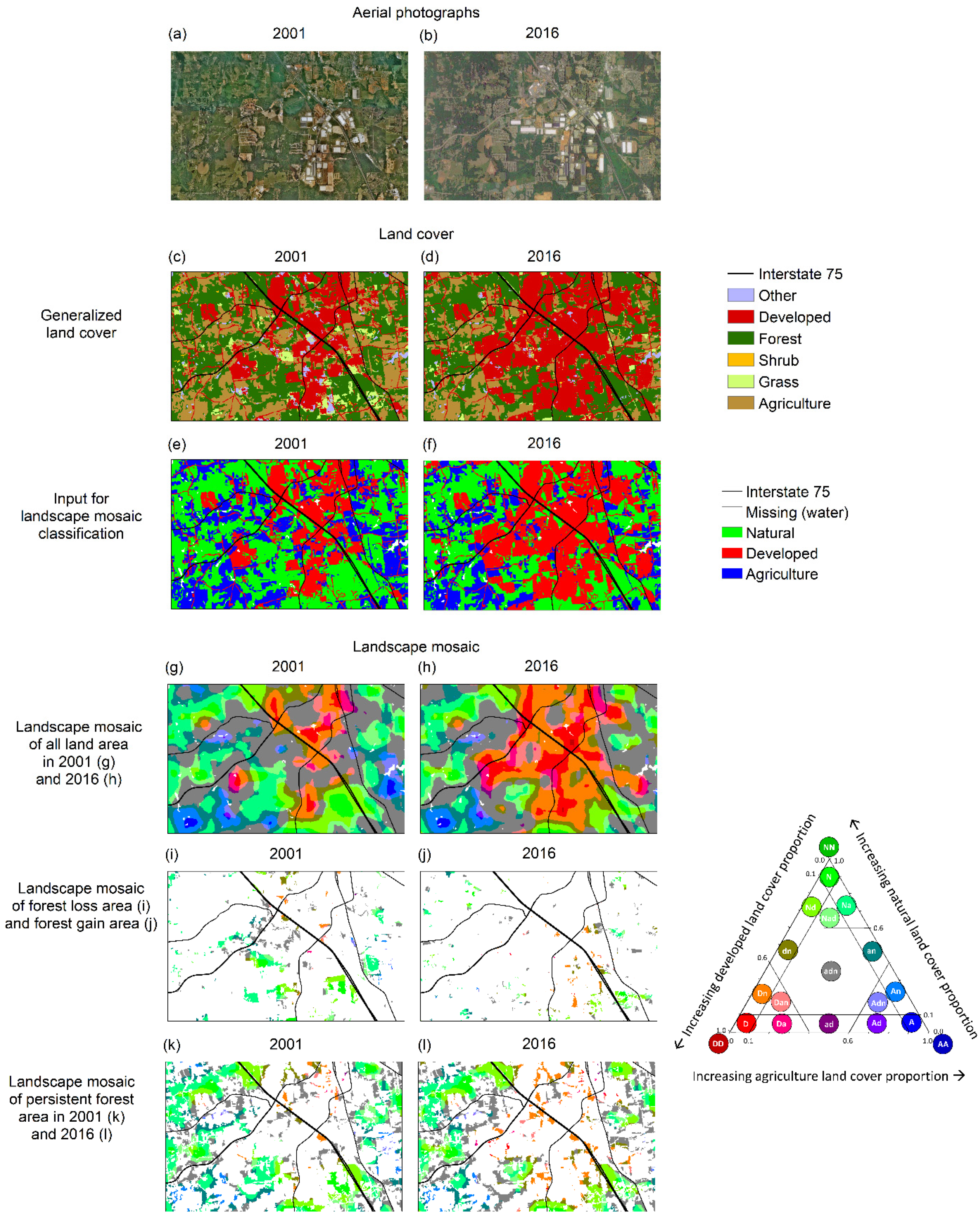
3.2. Land Cover Data

We used the CONUS NLCD land cover maps for 2001, 2011, and 2016 [34,35,36]. The NLCD maps were derived primarily from Landsat Thematic Mapper images and were produced at a spatial resolution of 0.09 ha with a thematic resolution of 16 land cover classes [7]. We defined forest land as the three NLCD upland forest cover classes and the woody wetlands cover class, developed land as the four NLCD developed cover classes (which incorporated impervious roads), and agriculture land as the NLCD pasture/hay and cultivated crop cover classes. For analysis of land cover change, we used the NLCD definitions of shrub land and grass land, and combined all remaining NLCD classes (water, ice, herbaceous wetland, and barren) into an “other” class. Changes of forest area in relation to landscape mosaic were evaluated for the time period 2001 to 2016. To support the analysis of change processes, we also evaluated changes of agriculture and developed land from 2001 to 2011. The NLCD maps defined the spatial extent of our study area.

3.3. Change Process Data

For comparisons with landscape mosaics in 2001, we evaluated neighborhood change processes from 2001 to 2011 from two sources. From the NAFD-ATT forest disturbance database [3] we identified the most recent major disturbance for each 0.09-ha location in the CONUS from 2001 to 2010. Disturbance by removals was defined as locations with tree stems mechanically severed from their trunks and where the land use was and remained forest. Disturbance by fire was defined as locations where evidence of forest fire existed regardless of cause, severity, or land use. Disturbance by stress was defined as locations where a stress-related spectral trend is evident in natural (primarily woody) vegetation environments, most likely resulting from insects, diseases, or drought. Each location was assigned one or more of those change processes according to their occurrence (yes or no) in a 4.41-ha neighborhood surrounding that location. Using the NLCD database [7], we evaluated the time period 2001 to 2011 to identify two types of land use change (yes or no; indicating a net increase in agriculture or developed land area) in the surrounding 4.41-ha neighborhood. The sum of the area exposed to all change processes was found to be larger than the total change area because more than one change process can occur near a given location, and a given change exposes all locations within its neighborhood. Hereafter, the five types of change processes are referred to as removal, fire, stress, agriculture, and developed.

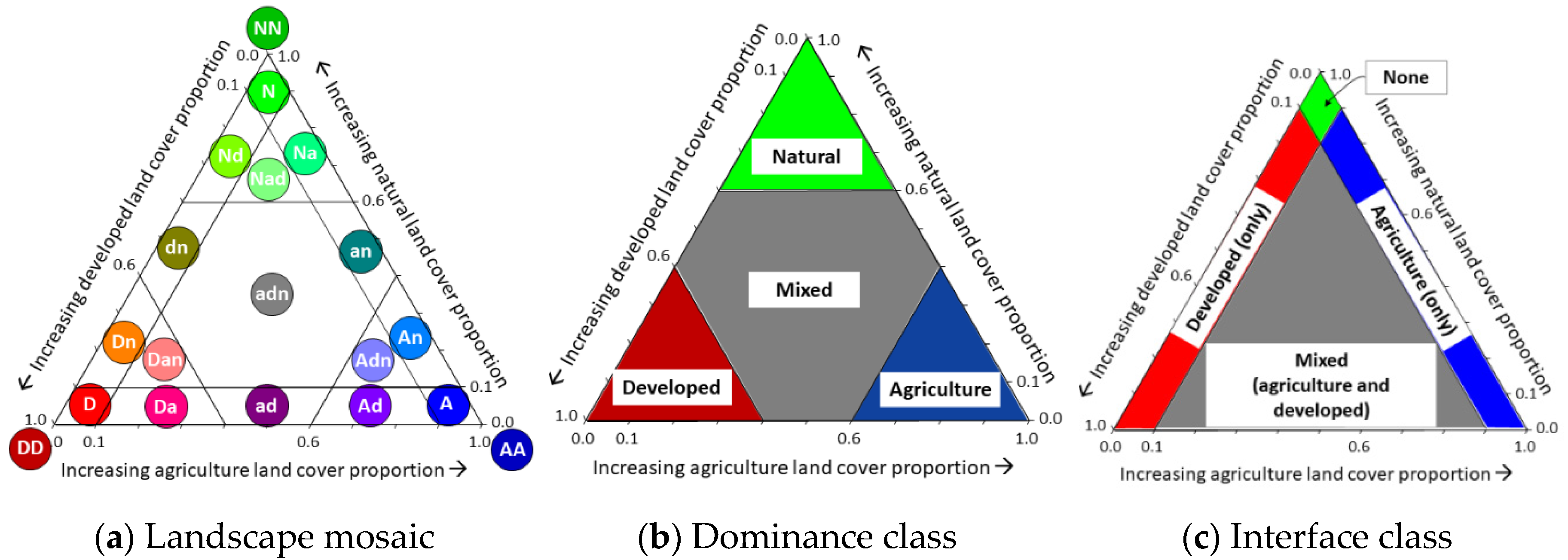
3.4. Landscape Mosaic Classification

The land cover maps were used to determine the landscape mosaic class of each 0.09-ha location in 2001 and 2016. The landscape mosaic classification of a given location is determined by the relative proportions of agriculture, developed, and natural (i.e., all other) land cover in the surrounding 65.61-ha neighborhood. Water is treated as missing data. The 19 mosaic classes were defined in a ternary chart by the threshold proportions of 0.1, 0.6, and 1.0 along each of the three axes (Figure 1a). The mosaic names indicate the presence (0.1 threshold), dominance (0.6), or uniqueness (1.0) of each land cover type. A lower-case letter (a—agriculture, d—developed, n—natural) in a mosaic name indicates a relative proportion of at least 0.1 but less than 0.6, and an upper-case letter (A, D, N) indicates a proportion of at least 0.6 but less than 1.0. Neighborhoods containing only one land cover (at the corners of the ternary chart) were classified as AA, DD, and NN, and a letter did not appear if the respective land cover proportion was less than 0.1. Landscape dominance was defined by reference to the 0.6 threshold values, yielding four dominance classes called natural, agriculture, developed, and mixed (Figure 1b). Landscape interfaces were defined by reference to the 0.1 threshold values, yielding four interface classes called agriculture, developed, mixed (i.e., both agriculture and developed), and none (i.e., neither agriculture nor developed) (Figure 1c). Hereafter, the three classifications are referred to as mosaic, dominance, and interface. An area near McDonough, Georgia (USA) (Figure 2a,b) illustrates the landscape mosaic classification and the geography of forest change in relation to mosaic change from 2001 to 2016. Land cover change in the neighborhood of a given location (Figure 2c,d) often resulted in a change of the mosaic for that location (Figure 2g,h). Overlaying forest masks for each year, the components of total forest change are forest loss from a mosaic class (Figure 2i), forest gain into a mosaic class (Figure 2j), and mosaic change in the neighborhood of persistent forest (compare Figure 2k,l).

4. Analysis

We summarized the mosaic changes for all locations by a transition matrix which has 19 state descriptors corresponding to the mosaic classes. To focus on forest dynamics in relation to mosaic changes, the mosaic maps were intersected with the forest maps in each year, and then combined across years. The corresponding transition matrix has 18 states, 17 of which indicate forest within a mosaic classes (by definition, forest does not occur in the mosaics AA and DD), and one which indicates the nonforest state. Exposures to forest change processes from 2001 to 2011 were summarized in relation to landscape mosaics in 2001. Recognizing that most land (and forest) area did not change over time, we constructed two metrics to help interpret the diagonal elements (i.e., the unchanged land) of the mosaic transition matrices from 2001 to 2016. The persistence of a mosaic (and of forest in a mosaic) was defined as the percentage of 2001 area that remained in the same class until 2016, and recruitment into that class was defined as the percentage of 2016 area that was not in that class in 2001. We used flow diagrams to visualize and summarize the transitions between classes that comprise the off-diagonal elements of a transition matrix. No statistical testing was performed since the data constituted a complete census of all land area. There was measurement error within the NLCD land cover maps [37] and the NAFD-ATT forest disturbance database but investigating measurement error propagation was beyond the scope of this study.

5. Results

5.1. Land Cover Change

The land cover transitions from 2001 to 2016 (

Table 1. Land cover change in the continental United States (CONUS), 2001 to 2016. The original 16 NLCD land cover classes were generalized to the six shown here; see Homer et al. (2020) for additional explanation.

	Land Cover in 2001
Land Cover in 2016	Forest	Grass	Shrub	Agriculture	Developed	Other 1	2016 Total
	km2
Forest	2,226,444	31,457	43,147	12,284	1	12,291	2,325,625
Grass	68,852	986,363	53,521	6823	1	2693	1,118,253
Shrub	71,484	36,030	1,647,723	4267	0	588	1,760,093
Agriculture	2634	32,908	6565	1,776,797	9	1750	1,820,663
Developed	7941	3928	3625	11,856	399,748	1268	428,366
Other	10,822	2201	1001	3856	1	318,383	336,264
2001 total	2,388,178	1,092,888	1,755,582	1,815,885	399,760	336,972	7,789,264

¹ Includes water, ice, herbaceous wetland, and barren land covers.

) are a necessary reference for results presented later. The developed land area increased by 7.2% and there was very little loss. While the net change of agriculture area was small in comparison (0.3%), the gross gain plus gross loss of agriculture area was equivalent to 4.6% of the original agriculture area. When examining transitions for one time period, a gain and loss of a given cover cannot occur at the same location; therefore the roughly 11.8% of total gross change of intensive land use (agriculture 4.6% plus developed 7.2%) indicates a substantial potential for geographic shifts of the landscape mosaic. Similarly, net forest loss was only 2.6% of the original forest area, but total forest change was equivalent to 11.0% of the original forest area, indicating substantial potential for changes of forest area in relation to the landscape mosaic.

The 15,494 km² gain of developed land from forest, shrub, or grass land with almost no reciprocal change suggests an expansion of developed-dominated landscapes. The net change of agriculture area was small but the gain from forest, shrub, or grass land was almost twice as large as the loss to those land types, suggesting an expansion of the agriculture-natural interface. However, there was almost five times more forest gain from agriculture than there was forest loss to agriculture, which suggests the forest area within agriculture-natural interfaces may have decreased even as the overall agriculture-natural interface area increased. A landscape analysis is required to evaluate the veracity of those suggestions.

5.2. Landscape Mosaic Change

The natural dominance class contained most of the total CONUS land area in both 2001 and 2016 (

Table 2. CONUS change of all land area, and of forest area only, from 2001 to 2016, by mosaic class.

			All Land Area			Forest Area
Dominance Class	Mosaic Class	Interface Class	2001	2016	Change	2001	2016	Change
			Thousand km2	Thousand km2	Percent	Thousand km2	Thousand km2	Percent
Agriculture	AA	Agriculture	103.5	103.8	0.3	-- a	--	--
	A	Agriculture	765.7	775.1	1.2	6.1	5.9	−3.6
	Ad	Mixed	61.3	65.0	6.0	0.7	0.7	0.0
	An	Agriculture	606.0	602.5	−0.6	61.0	58.0	−5.0
	Adn	Mixed	42.4	42.5	0.2	4.3	4.1	−3.7
Developed	DD	Developed	23.6	25.3	7.1	--	--	--
	D	Developed	56.4	66.2	17.5	0.6	0.7	21.5
	Dn	Developed	59.9	68.6	14.7	7.5	8.7	17.1
	Da	Mixed	12.2	15.7	28.5	0.1	0.2	28.6
	Dan	Mixed	7.2	8.4	16.8	0.6	0.7	19.1
Natural	NN	None	2976.6	2943.5	−1.1	932.4	896.4	−3.9
	N	None	1357.1	1362.3	0.4	721.3	713.6	−1.1
	Na	Agriculture	642.2	626.3	−2.5	317.0	302.8	−4.5
	Nd	Developed	200.8	209.8	4.5	109.1	111.9	2.6
	Nad	Mixed	57.5	58.5	1.7	33.1	32.9	−0.6
Mixed	ad	Mixed	12.0	14.1	17.1	0.2	0.2	9.4
	an	Agriculture	467.9	456.6	−2.4	134.0	126.8	−5.4
	dn	Developed	41.8	46.0	10.0	14.1	15.6	10.8
	adn	Mixed	155.9	161.6	3.6	46.1	46.4	0.6
All classes			7650.1	7651.7 b		2388.2	2325.6	−2.6 c

^a By definition, there is no forest in the DD or AA mosaics. ^b Total differs from 2001 because water area is excluded from both totals. ^c Change from 2001 to 2016 indicates net loss of forest area.

). For later reference, note that the relationship between the mosaic, dominance, and interface classes (Figure 1) is shown in Table 2. The mosaics in the developed dominance class contained the least area but exhibited the largest percentage increases, and there was a net increase in the area of all mosaics comprising the developed interface class. The diagonal elements of the 19 × 19 mosaic class transition matrix (Supplemental Table S1) were summarized by persistence and recruitment. With one exception (Nd), the most persistent mosaics were those that were not in an agriculture or developed interface, and the least persistent mosaics were those in the mixed interface (Figure 3). Recruitment was highest in the developed interface where expansion of the developed interface area is indicated by high persistence in some mosaics (e.g., Nd, Ad, Dn) and high turnover rates in transitional landscapes are indicated by low persistence in other mosaics (e.g., Dan, Da, ad, dn).

The flow diagrams of the off-diagonal elements of the mosaic transition matrix are shown in Supplemental Figure S1. With a few exceptions, most of the changes of mosaic class area occurred within dominance classes. In the developed dominance class, mosaic changes indicated a concentration of area into the D and DD mosaic classes. In contrast to other dominance classes, the gains in the developed dominance class were distributed more evenly among mosaics both within and outside of that dominance class, and there was relatively little loss from the developed dominance class. The mixed dominance class exhibited a more even distribution of mosaic loss and gain within and outside of that class, which is consistent with the definition of the mixed dominance class as a transitional state between the other three dominance classes.

Flow diagrams of CONUS land area change among dominance classes and among interface classes are shown in Figure 4. There was a net gain of area in the developed dominance class, and a net loss of area in the natural dominance class (Figure 4a). The mixed dominance class was transitional in the sense that most of the increase in the developed dominance class came from the mixed dominance class, and most of the decrease in the natural dominance class went to the mixed dominance class. The mixed dominance class was also transitional with respect to changes between the natural and agriculture dominance classes, but unlike the developed dominance class, there were changes in both directions. The expansion of developed landscapes was also evident in the transitions among interface classes (Figure 4b).

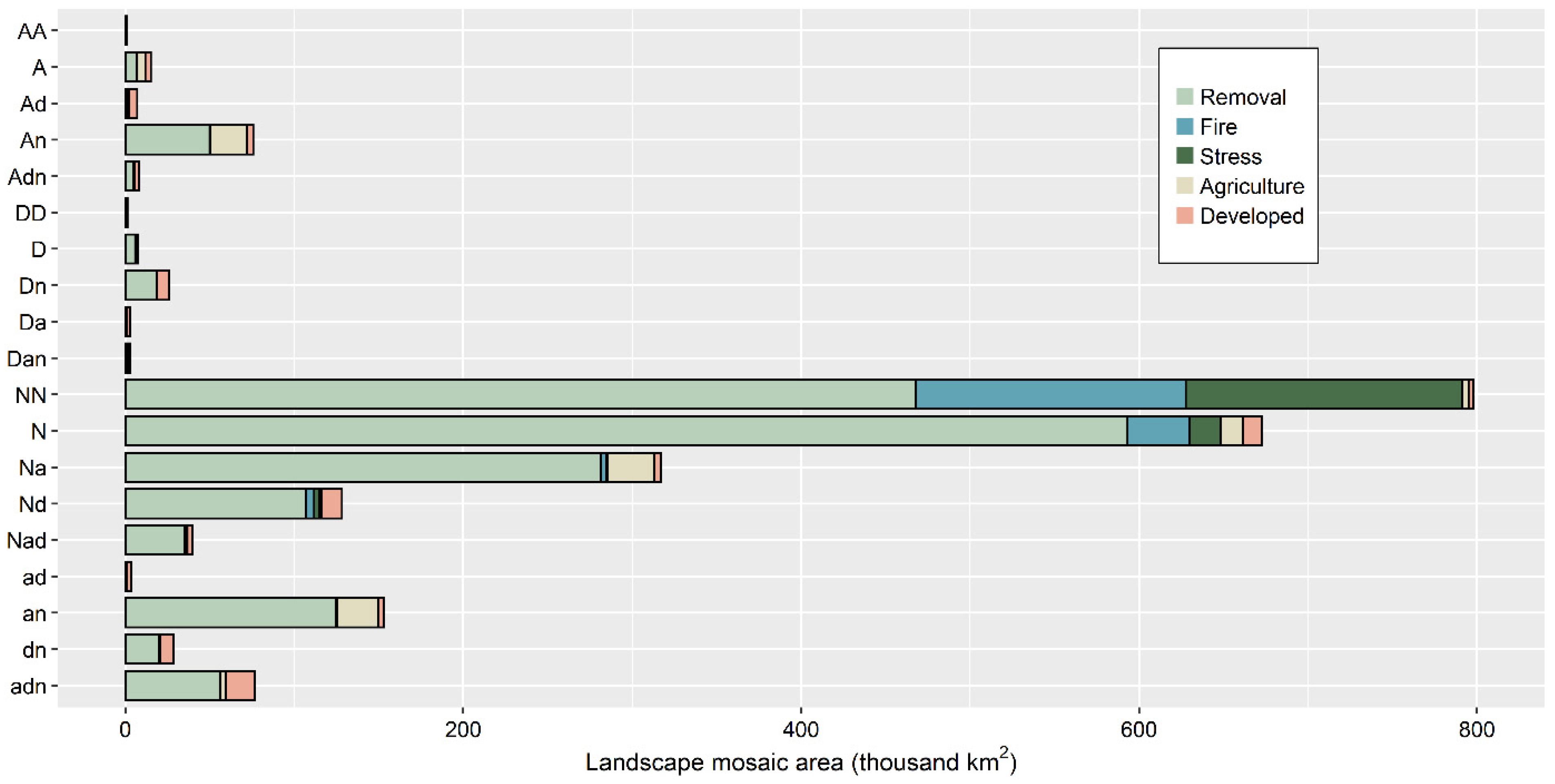
5.3. Change Processes in Landscape Mosaics

The area of each mosaic that was exposed to different types of change processes within a 4.41-ha neighborhood varied substantially among mosaics (Figure 5). The relatively large area of change in the natural dominance class was not surprising because those mosaics contained most of the total area and most of the forest area in 2001 (Table 2). Removal was the most frequent type of change process and increases of agriculture or developed land uses were the least frequent. Exposure to fire or stress was common only in the NN and N mosaics. Exposure to increased agriculture land use was concentrated in the agriculture interface, and with one exception (mosaic N) the exposure to increased developed land use was concentrated in the developed interface.

To account for differences in the total area of each mosaic class, the class area that was exposed to each type of change process was expressed as the percent of total class area (

Table 3. CONUS shares of landscape mosaic area in 2001 that were exposed to five types of change processes in a surrounding 4.41 ha neighborhood by 2011. Changes are not mutually exclusive; i.e., a given neighborhood may contain more than one type of change. Excludes area that was water in 2001.

		Type of Change Process, 2001 to 2011
Landscape Mosaic Class	Area in 2001	Forest Removal	Forest Fire	Forest Stress	Increased Agriculture	Increased Developed
	Thousand km2	Percent of Area in 2001
AA	104	—— a	— b	—	——	——
A	769	——	—	—	——	——
Ad	62	2.5	——	—	——	8.2
An	613	8.1	——	—	3.5	——
Adn	43	11.0	——	—	1.8	5.6
DD	24	5.1	——	—	—	—
D	58	10.2	——	—	—	2.3
Dn	62	29.5	——	——	——	11.4
Da	12	6.7	——	—	——	14.2
Dan	7	21.3	——	—	——	16.1
NN	3011	15.5	5.3	5.4	——	——
N	1375	43.1	2.7	1.4	——	——
Na	652	43.2	——	——	4.3	——
Nd	213	50.1	2.3	1.4	——	5.8
Nad	59	59.5	——	——	2.0	4.6
ad	12	4.6	——	—	——	22.7
an	474	26.3	——	—	5.1	——
dn	44	44.6	——	——	——	17.8
adn	161	34.7	——	—	2.2	10.7
All classes	7757	22.9	2.7	2.4	1.3	1.2

^a “——” indicates < 1, ^b “—” indicates < 0.1.

). More than one-half of the area of two mosaics (Nd, Nad) was exposed to change by removal, and that fraction exceeded one-third for four additional mosaics (N, Na, dn, and adn). Only in the NN mosaic was more than 5% of total area exposed to fire or stress, while values less than 1% were typical of almost all other mosaic classes. Exposure to increased agriculture or developed land uses exceeded 1% of total area primarily in the interface classes that contain at least 10% of the respective land cover.

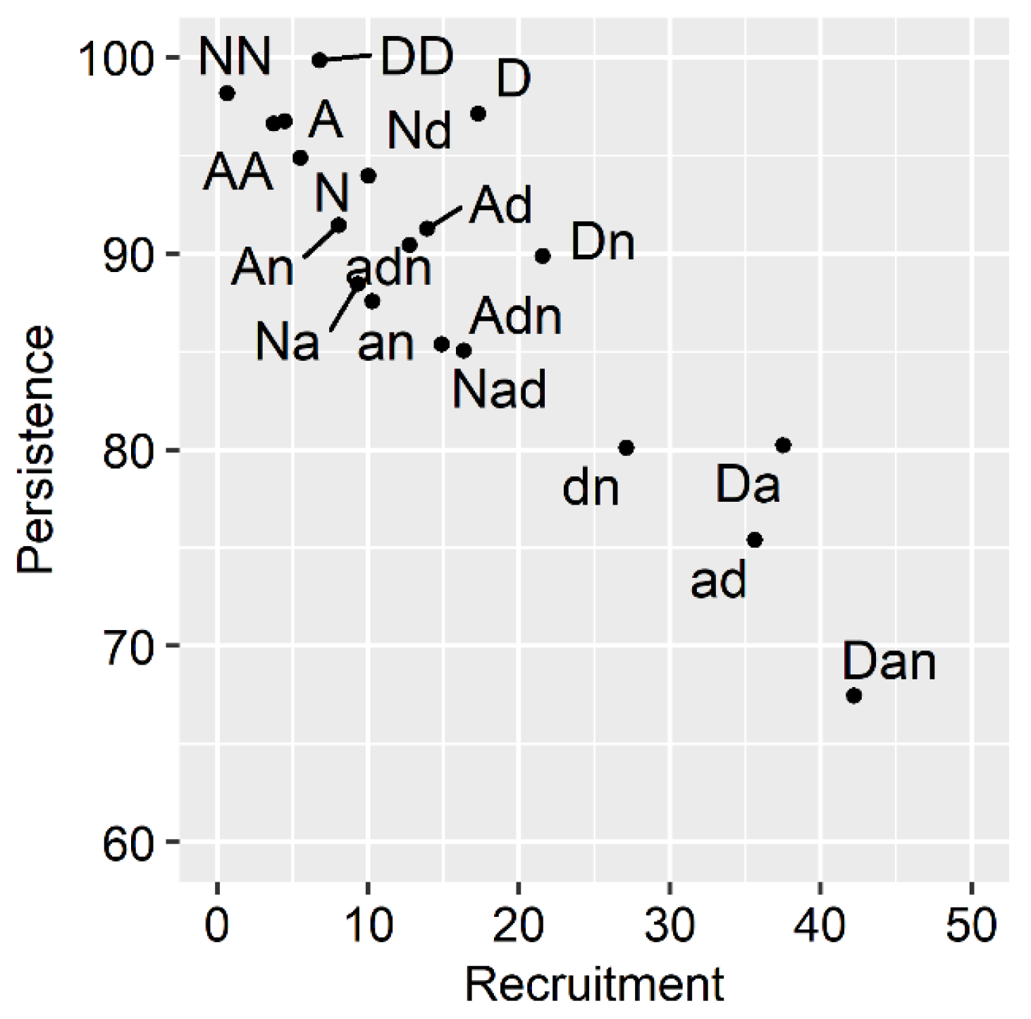
5.4. Forest and Landscape Mosaic Change

The forest area was concentrated in the mosaics comprising the natural dominance class, where most of the forest changes occurred (Table 2; Supplemental Figure S2). As a percent of forest area in 2001, increases of 17 to 29% occurred in the developed dominance class (D, Dn, Da, Dan), and increases of up to 11% were common in the mosaics of the developed interface. Decreases were common in the agriculture dominance and interface classes, unless the mosaic was also in the developed interface class. Compared to all land area, the persistence of forest area in mosaic classes was generally lower, and the recruitment was generally higher, because forest change involved both gains and losses, as well as changes of landscape mosaic for the persistent forest area (Supplemental Figure S3).

Forest changes in relation to mosaics were further evaluated by partitioning persistence and recruitment into components attributable to forest gain, forest loss and the shifting landscape mosaic (

Table 4. Components of forest area instability and recruitment from 2001 to 2016, by mosaic class. Recruitment and instability (the complement of persistence) are defined in the text. The components of total change include either forest gain or forest loss, and the change of mosaic class for area that was forest at both dates. The AA and DD mosaics are not shown because they contain no forest.

	Forest Instability			Forest Recruitment
Mosaic	Forest Loss	Mosaic Change	Total Change	Forest Gain	Mosaic Change	Total Change
	Percent	Percent	Percent	Percent	Percent	Percent
A	2.7	4.7	7.5	1.6	2.4	4.1
Ad	5.1	9.3	14.4	2.3	12.1	14.4
An	3.2	5.9	9.1	2.4	2.0	4.4
Adn	4.5	12.5	17.0	2.7	11.1	13.8
D	9.8	0.6	10.5	1.6	24.7	26.3
Dn	10.7	1.9	12.6	1.6	23.8	25.3
Da	13.0	14.0	27.0	3.5	39.7	43.2
Dan	11.7	24.2	35.8	3.0	43.1	46.1
NN	7.2	0.8	8.0	3.1	1.2	4.3
N	7.5	2.8	10.2	6.0	3.3	9.3
Na	5.5	7.3	12.8	4.8	3.9	8.7
Nd	6.9	2.9	9.8	3.9	8.2	12.1
Nad	5.9	11.4	17.2	4.2	12.6	16.8
ad	10.7	15.7	26.5	2.9	29.9	32.8
an	4.3	7.9	12.2	3.6	3.6	7.2
dn	9.6	10.3	19.9	2.2	25.5	27.7
adn	6.3	6.6	12.9	3.5	9.9	13.4
All forest	6.8	3.2	10.0	4.3	3.3	7.6

). Persistence was expressed as “instability” (i.e., 1 minus persistence) of the 2001 forest area, and recruitment referred to gains into a mosaic class between 2001 and 2016. Forest loss rates were highest (10–13%) in the mosaics comprising the developed dominance class, lowest (3–5%) in those comprising the agriculture dominance class, and intermediate (6–7%) in those comprising the natural dominance class. In the mixed dominance class, the rate of forest loss was generally lower for the mosaics which contain at least 10% agriculture land than for those which contain at least 10% developed land. The rate of change of mosaic class for the persistent forest depended more on interface class than on dominance class. The rate of a mosaic change was lowest (1–3%) in mosaic classes that are not in an interface (A, D, NN, N), and generally higher (9–24%) in the interface class that contains at least 10% of both agriculture and developed cover (e.g., Adn, Dan, Nad, Ad, Da, ad). All types of change, total instability and total recruitment were typically high in the mosaic classes with at least 10% developed cover, where most of the changes were due to the shifting mosaic. The large forest recruitment without forest gain into the mosaic classes with at least 10% developed cover is evidence that expanding developed landscapes assimilated more of the persistent forest from 2001 to 2016. The supplemental material contains the 18 × 18 forest and mosaic transition matrix (Supplemental Table S2) and the flow diagrams of the off-diagonal elements of that matrix (Supplemental Figure S2).

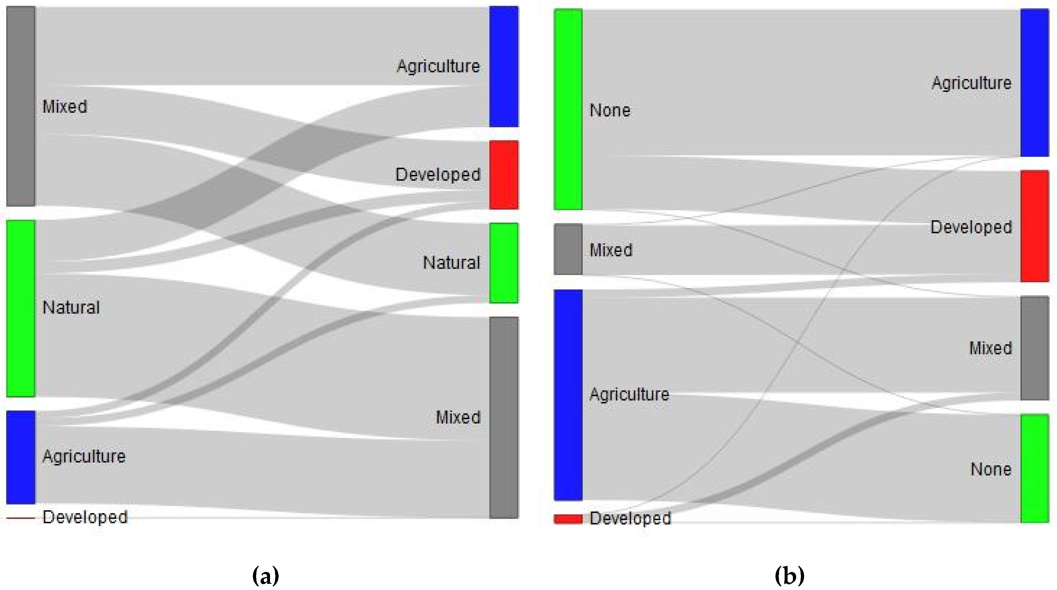
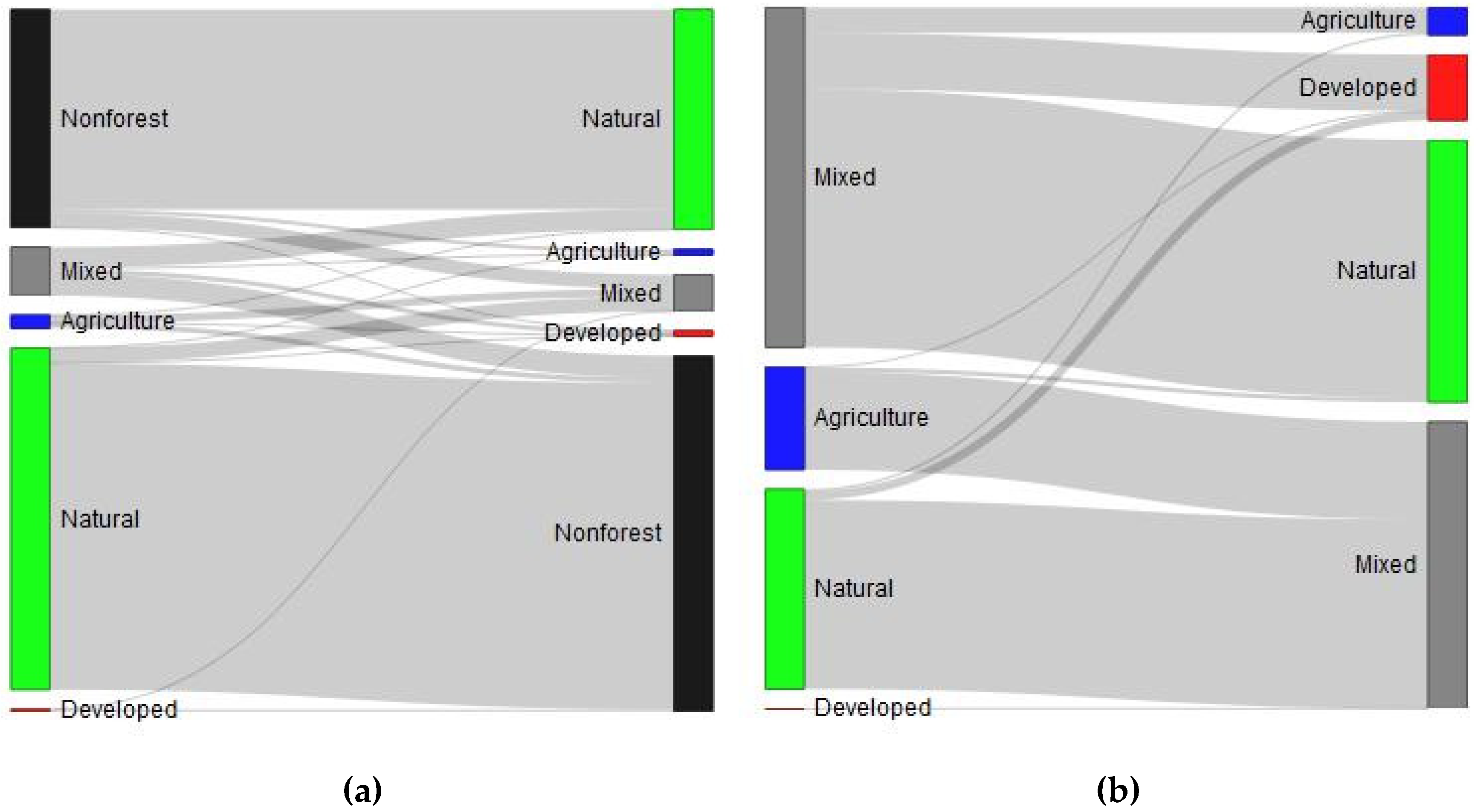
5.4.1. Forest and Landscape Dominance Change

The transition matrix of forest change in relation to landscape dominance class (Supplemental Table S3) clarifies the contributions of dominance change to total forest change. Compared to an overall 2.6% net loss of forest area, which approximates the percentage losses in the natural and mixed dominance classes, there was a net loss of 4.7% of forest in the agriculture dominance class and a net gain of 17.7% in the developed dominance class (

Table 5. Forest area change by landscape dominance class in the continental United States, 2001 to 2016. In addition to the percent of total gross change attributable to forest loss or gain (as shown), the percent of total gross change attributable to the shifting landscape mosaic can be obtained by subtraction from 100. Nonforest statistics are shown for comparison.

	Total Area		Net Change	Gross Loss		Gross Gain
Dominance Class	2001	2016		Total Change	Forest Loss	Total Change	Forest Gain
	Thousand km2		Percent	Thousand km2	Percent a	Thousand km2	Percent a
Agriculture	72	69	−4.7	6	39	3	62
Developed	9	10	17.7	1	99	3	7
Natural	2113	2058	−2.6	156	95	100	91
Mixed	194	189	−2.8	22	45	17	39
All forest	2388	2326	−2.6	184	88	122	81
For comparison:
Nonforest	5401	5464	1.2	162	100	99	100

^a Percent of total change area.

). Almost all forest change in the natural dominance class was due to forest gain and loss. In contrast, in the developed dominance class most of the loss was attributable to forest loss but most of the gain was due to the shifting mosaic. The opposite occurred in the agriculture dominance class, for which most of the loss was due to the shifting mosaic and most of the gain was due to forest gain. Roughly 40% of forest change in the mixed dominance class was attributable to forest loss and gain. Considering forest change in all dominance classes, the shares of change attributable to forest loss and gain (88% and 81%) approximated the shares in the natural dominance class (95% and 91%) because the natural dominance class contained 84% of the total change area.

In terms of forest area flows between landscape dominance classes and nonforest (Figure 6a) the most important flows were reciprocal between nonforest and forest in the natural dominance class. In terms of dominance change of persistent forest (Figure 6b), the most important flows were reciprocal between the natural and mixed dominance classes which favored an increase of forest area in the natural dominance class. Reciprocal flows between the agriculture and mixed dominance classes favored a decrease of forest area in the agriculture dominance class. The developed dominance class was essentially a “sink” with forest area flows coming from (in decreasing order of area) the mixed, natural, and agriculture dominance classes.

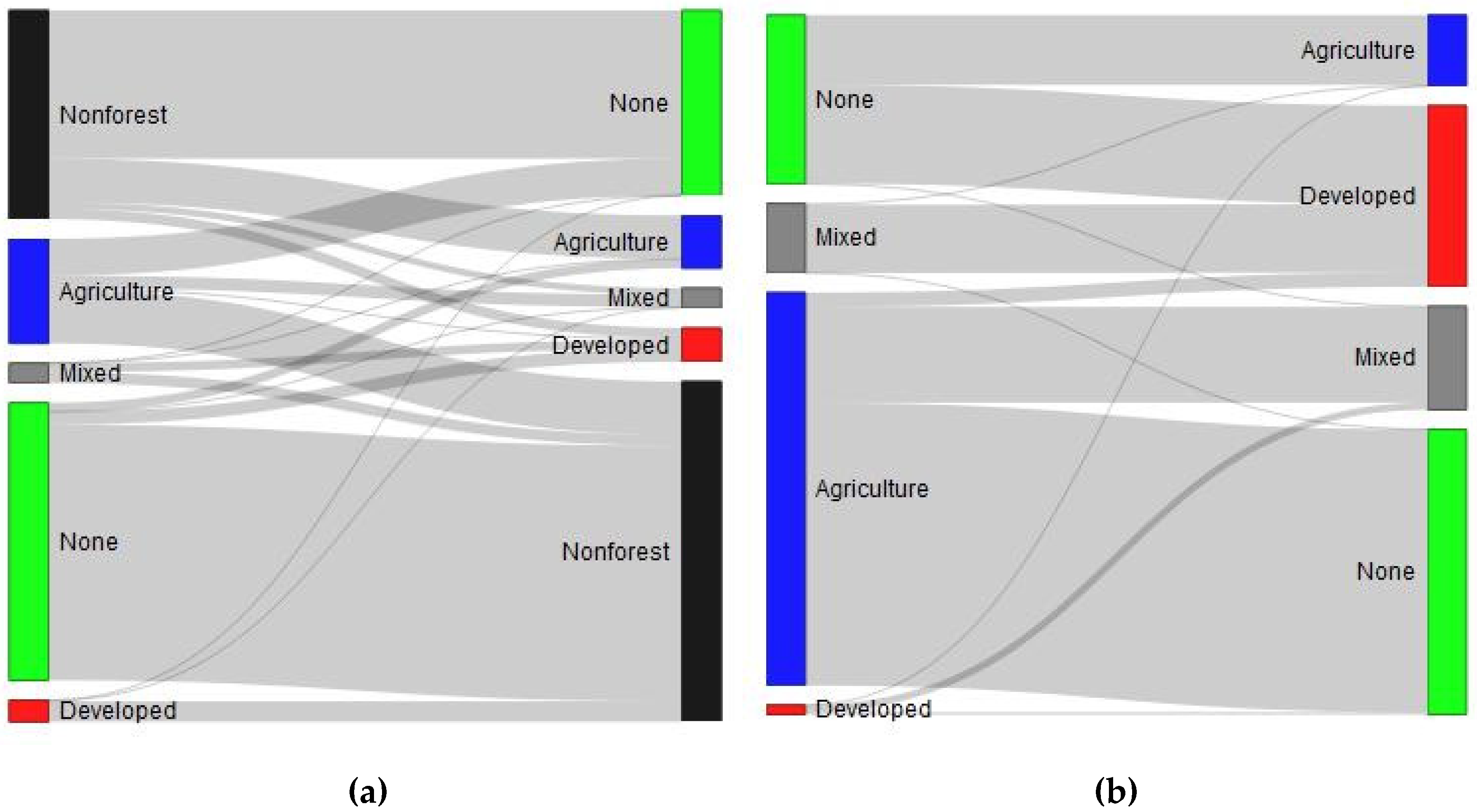
5.4.2. Forest and Landscape Interface Change

The transition matrix of forest change in relation to interface class (Supplemental Table S4) clarifies the contributions of interface change to total forest change. Overall results (

Table 6. Forest area change by interface class in the continental United States, 2001 to 2016. In addition to the percent of total gross change attributable to forest loss or gain (as shown), the percent of total gross change attributable to the shifting landscape mosaic can be obtained by subtraction from 100. Comparable statistics for nonforest areas are shown in Table 5.

	Total Area		Net Change	Gross Loss		Gross Gain
Interface Class	2001	2016		Total Change	Forest Loss	Total Change	Forest Gain
	Thousand km2		Percent	Thousand km2	Percent a	Thousand km2	Percent a
Agriculture	518	494	−4.8	50	51	25	82
Developed	131	137	4.4	10	94	16	30
Mixed	85	85	0.1	9	55	10	33
None	1654	1610	−2.6	132	92	88	80
All forest	2388	2326	−2.6	201	80	139	71

^a Percent of total change area.

) were broadly like changes in relation to dominance class (Table 5), except the increase in the developed interface was smaller than the increase in the developed dominance class and the share of gain attributable to forest gain was larger. There was almost no change in the forest area in the mixed interface class. Flow diagrams of forest change in relation to landscape interface and nonforest (Figure 7a) indicate the most important flows were between nonforest and the agriculture or “none” interface classes. For the interface changes of attributable to the shifting mosaic (Figure 7b), the most important flows were from the agriculture interface class, to the “none” class (resulting from a loss of agriculture land), and to the mixed class (resulting from a gain of developed land). As was the case for developed dominance, the developed interface class was essentially a sink, with almost all of the flow of forest area coming from the “none” and mixed classes; the former was the result of increased developed land and the latter resulted from a loss of agriculture land.

6. Discussion

The geography of change matters, and land managers and planners need to know the landscape context within which changes occurred or would be expected. In this study of landscape changes from 2001 to 2016, land cover changes resulted in a change of landscape mosaic for an area equivalent to 5.3% of the total area of the continental United States (excluding water area). Whether measured by forest-nonforest transitions or by the shifting landscape mosaic of persistent forest, forest dynamics within those landscapes was a major contributor to overall change. From 2001 to 2016, the forest area decreased by 2.6%, but the total gross change (11.0%) was more than four times larger than net change. An additional 3.2% of the persistent forest experienced a change of landscape mosaic. Thus, landscape mosaic change affected an area equivalent to 29% of the total gross change and increased the overall rate of change from 11.0% to 14.2% of the total forest area in 2001. To put those numbers in perspective, the equivalent average annual rate of change (~0.9%) is roughly the same as the annual North America forest loss rates [1,2].

The nature of land cover data makes it difficult to use that data alone to establish whether the forest change was temporary versus permanent, or natural versus anthropogenic, but information about the landscape context of forest change provides some of the best evidence to date that most of the change was temporary. The land cover data alone (Table 1) support the conclusion [1] that most forest canopy cover change is temporary and due to pervasive forestry operations. Of the 161,733 km² of gross forest cover loss, 87% was converted to shrub or grass cover, and 75% of the gross forest cover gain was conversion from shrub or grass covers which typically appear after forestry operations. The contextual information provided by the landscape mosaic classification strengthens that evidence by showing that most forest loss and gain occurs in landscapes containing relatively little agriculture or developed land. However, we also found evidence that a substantial area of forest loss was probably permanent simply because it occurred in developed landscapes, and that more forest area was assimilated into newly developed landscapes where the likelihood of future forest loss is higher. If present trends of increases in human population and development continue, then there will be more permanent conversions and thus less forest area available to support not only forestry operations but also all other forest-based amenities such as water and recreation [25]. Over the long term, the sustainability of all forest amenities depends on sustaining the forested landscapes within which the forest can be used as forest.

Our results concerning exposure to forest change processes are generally consistent with earlier studies in that change was a common event, and forest removal was the most important type of change [1,3,5]. With one exception, we found that exposure to fire and stress was common only in natural landscapes. We attribute the exception (mosaic Nd) mosaic to events occurring near isolated roads (a type of developed land cover) in mostly forested landscapes [38]. The relatively large exposures to forest removal in many of the mosaic classes that were not dominated by natural cover are explained by noting that expansion of agriculture and developed land area often requires forest removal. We found that exposure to increased agriculture or developed land uses occurred primarily in landscapes that were already agricultural or developed landscapes, lending additional support to the argument that intensified land use is not a major component of forest dynamics in remote areas.

The extensive human “footprint” may consider many types of human activities [39,40]. The landscape mosaic classification can be viewed as the component of the human footprint which identifies the signals of intensive land uses near otherwise natural areas. Typical investigations of such interface areas have focused on the expansion of developed area and the wildland-urban interface where trees co-occur with houses [41,42]. Our results for expansion of the developed interface class are generally consistent with those investigations, but we also found evidence of urban expansion into agricultural landscapes where trees also occur. Several aspects of our approach could be useful in future studies of various types of interface. Unlike current procedures for mapping wildland-urban interface [42], the mosaic is mapped at a fixed (and higher) spatial resolution (equal to the resolution of the land cover data), stationarity need not be assumed within the housing density regions which define the wildland-urban interface classes, and the modifiable area unit problem [43] is postponed until after the mosaics are mapped. With landscape mosaics as a basis, the housing density thresholds used to define the wildland-urban interface (or other aspects of the human footprint) can be incorporated later as a refinement of the landscape mosaic map. Use of the same landscape mosaic classification for different refinements permits, for example, consistent analysis of the wildland-urban, agriculture-urban, and wildland-agriculture interfaces, which would be important when investigating land use impacts on broad-scale spatial processes such as pollination or the spread of invasive species. Even without further analysis, temporal animations of the shifting landscape mosaic help to visualize the type, location, scale, and velocity of changes in the human footprint (see Supplemental Videos).

This study addressed questions about the causes and consequences of forest and landscape pattern changes at regional scale. The synoptic data we used are essential for assessing landscape patterns consistently over such a large area and are a first step to guide broad policy [24]. A synoptic assessment helps to refine the scope of future research by identifying where some questions should be asked in more detail, and why the investigation is important in terms of local societal values and resource management opportunities. Predicting and managing the local impacts of change will always depend on circumstances such as the specific landscape history [44], the cause of the change [45], and the specific question or species that is being addressed [46]. However, such detailed investigations typically require more detailed spatial and thematic data that are either unavailable or inconsistent over large regions. One can argue the relative merits of up-scaling versus down-scaling approaches to address a given question across scales, but as a practical matter neither approach can stand alone if cross-disciplinary integration is envisioned. For that purpose, we believe the landscape mosaic classification can provide a consistent synoptic and local framework for spatial analysis of land use change, one which can accommodate a variety of disciplinary perspectives and investigations.

We can suggest several paths for future research and applications of landscape mosaics. Our focal class was forest, but the same approach could be used to explore change of agriculture land which is another important resource that is threatened by development [47,48]. Alternatively, point (or field plot) data could be attributed with mosaic classes to explore temporal changes of that data in relation to landscape context [49]. The demonstrated dependence of forest change on landscape mosaic suggests the use of landscape mosaics as independent variables in models of future forest change. Alternatively, the “spatial credibility” of predicted land use changes could be validated by comparing historical evolutions with the predicted future evolution of the landscape mosaic. Markov chain models of landscape mosaic change may be useful when there are no other predictor data [50]. For that application, the 18 × 18 transition matrix that we used to summarize forest change simply adds a mosaic label to the forest states in a traditional 2 × 2 (forest-nonforest) transition matrix. Using methods and terminology from Hill et al. [51], the nonforest state is “substrate,” and a Markov chain analysis of mosaic “community dynamics” provides many descriptors of landscape and forest dynamics. For example, relative convergence rates towards steady state distributions of landscape mosaics alone and forest within landscape mosaics indicate the sustainability of forest area within a shrinking area of forested landscapes [11]. We specified a mosaic neighborhood size that is relevant to understanding local land use changes in the United States. However, the landscape mosaic is scale-dependent, and the neighborhood size is simply a tuning parameter. Larger (or smaller) neighborhood sizes will characterize lower (or higher) spatial frequencies of land cover variance (Supplemental Figure S4). Following a multi-scale analysis, a “scale domain” at a given location is a range of neighborhood size over which the mosaic class is invariant. Discontinuities on a map of scale domains could represent locations of mosaic “tipping points” and indicate their spatial scales. In principle, a ternary classification can be applied to any categorical map, and software is available to use other data and threshold values [52]. Our research demonstrates that it is feasible and informative to examine forest change within a changing landscape context at a high spatial resolution and at a continental extent.

References

1. Masek, J.G.; Huang, C.; Wolfe, R.; Cohen, W.; Hall, F.; Kutler, J.; Nelson, P. North American forest disturbance mapped from a decadal Landsat record. Remote. Sens. Environ. 2008, 112, 2914–2926. [Google Scholar] [CrossRef]
2. Hansen, M.C.; Stehman, S.V.; Potapov, P.V. Quantification of global gross forest cover loss. Natl. Acad. Sci. USA 2010, 107, 8650–8655. [Google Scholar] [CrossRef] [PubMed] [Green Version]
3. Schleeweis, K.G.; Moisen, G.G.; Schroeder, T.A.; Toney, C.; Freeman, E.A.; Goward, S.N.; Huang, C.; Dungan, J.R. US National Maps Attributing Forest Change: 1986–2010. Forestry 2020, 11, 653. [Google Scholar] [CrossRef]
4. Sommerfeld, A.; Senf, C.; Buma, B.; D’Amato, A.W.; Després, T.; Díaz-Hormazábal, I.; Fraver, S.; Frelich, L.E.; Gutiérrez, Á.G.; Hart, S.J.; et al. Patterns and drivers of recent disturbances across the temperate forest biome. Nat. Commun. 2018, 9, 4355. [Google Scholar] [CrossRef] [PubMed]
5. Cohen, W.B.; Yang, Z.; Stehman, S.V.; Schroeder, T.A.; Bell, D.M.; Masek, J.G.; Huang, C.; Meigs, G.W. Forest disturbance across the conterminous United States from 1985–2012: The emerging dominance of forest decline. For. Ecol. Manag. 2016, 360, 242–252. [Google Scholar] [CrossRef]
6. Curtis, P.G.; Slay, C.M.; Harris, N.L.; Tyukavina, A.; Hansen, M.C. Classifying drivers of global forest loss. Science 2018, 361, 1108–1111. [Google Scholar] [CrossRef] [PubMed]
7. Homer, C.; Dewitz, J.; Jin, S.; Xian, G.; Costello, C.; Danielson, P.; Gass, L.; Funk, M.; Wickham, J.; Stehman, S.; et al. Conterminous United States land cover change patterns 2001–2016 from the 2016 National Land Cover Database. ISPRS J. Photogramm. Remote Sens. 2020, 162, 184–199. [Google Scholar] [CrossRef]
8. Oswalt, S.N.; Smith, W.B.; Miles, P.D.; Pugh, S.A. Forest Resources of the United States, 2017: A Technical Document Supporting the Forest Service 2020 RPA Assessment; Gen. Tech. Rep. WO-97; U.S. Department of Agriculture, Forest Service, Washington Office: Washington, DC, USA, 2019; 223p. [CrossRef] [Green Version]
9. Nelson, M.D.; Riitters, K.H.; Coulston, J.W.; Domke, G.M.; Greenfield, E.J.; Langner, L.L.; Nowak, D.J.; O’Dea, C.B.; Oswalt, S.N.; Reeves, M.C.; et al. Defining the United States Land Base: A Technical Document Supporting the USDA Forest Service 2020 RPA Assessment; Gen. Tech. Rep. NRS-191; U.S. Department of Agriculture, Forest Service, Northern Research Station: Madison, WI, USA, 2020; 70p. [CrossRef]
10. Coulston, J.W.; Reams, G.A.; Wear, D.N.; Brewer, C.K. An analysis of forest land use, forest land cover and change at policy-relevant scales. Forestry 2013, 87, 267–276. [Google Scholar] [CrossRef]
11. Riitters, K.H.; Wickham, J.D.; Wade, T.G. An indicator of forest dynamics using a shifting landscape mosaic. Ecol. Indic. 2009, 9, 107–117. [Google Scholar] [CrossRef]
12. Pacheco, A.P.; Claro, J.; Fernandes, P.M.; De Neufville, R.; Oliveira, T.M.; Borges, J.G.; Rodrigues, J.C. Cohesive fire management within an uncertain environment: A review of risk handling and decision support systems. For. Ecol. Manag. 2015, 347, 1–17. [Google Scholar] [CrossRef]
13. Vicente, J.R.; Alves, P.; Randin, C.; Guisan, A.; Honrado, J.P. What drives invasibility? A multi-model inference test and spatial modelling of alien plant species richness patterns in northern Portugal. Ecography 2010, 33, 1081–1092. [Google Scholar] [CrossRef]
14. Vilà, M.; Ibáñez, I. Plant invasions in the landscape. Landsc. Ecol. 2011, 26, 461–472. [Google Scholar] [CrossRef]
15. Riitters, K.; Potter, K.; Iannone, B.V.; Oswalt, C.M.; Fei, S.; Guo, Q. Landscape correlates of forest plant invasions: A high-resolution analysis across the eastern United States. Divers. Distrib. 2017, 24, 274–284. [Google Scholar] [CrossRef] [Green Version]
16. Silva, R.G.; Zenni, R.D.; Rosse, V.P.; Bastos, L.S.; Berg, E.V.D. Landscape-level determinants of the spread and impact of invasive grasses in protected areas. Biol. Invasions 2020, 22, 3083–3099. [Google Scholar] [CrossRef]
17. Sweeney, B.W.; Newbold, J.D. Streamside Forest Buffer Width Needed to Protect Stream Water Quality, Habitat, and Organisms: A Literature Review. JAWRA J. Am. Water Resour. Assoc. 2014, 50, 560–584. [Google Scholar] [CrossRef]
18. Wolf, K.L. Freeway roadside management: The urban forest beyond the white line. J. Arboric. 2003, 29, 127–136. [Google Scholar]
19. Buist, L.J.; Hoots, T.A. Recreation opportunity spectrum approach to resource planning. J. For. 1982, 80, 84–86. [Google Scholar] [CrossRef]
20. Sommers, W.T. The emergence of the wildland-urban interface concept. For. Hist. Today Fall 2008, 12–18. [Google Scholar]
21. Lewis, D.J. An economic framework for forecasting land-use and ecosystem change. Resour. Energy Econ. 2010, 32, 98–116. [Google Scholar] [CrossRef] [Green Version]
22. Reichelderfer, K.; Boggess, W.G. Government Decision Making and Program Performance: The Case of the Conservation Reserve Program. Am. J. Agric. Econ. 1988, 70, 1–11. [Google Scholar] [CrossRef] [Green Version]
23. Malmsheimer, R.W.; Bowyer, J.L.; Fried, J.S.; Gee, E.; Izlar, R.; Miner, R.A.; Munn, I.A.; Oneil, E.; Stewart, W.C. Managing forests because carbon matters: Integrating energy, products, and land management policy. J. For. 2011, 109, S7–S50. [Google Scholar]
24. O’Neill, R.V.; Hunsaker, C.T.; Jones, K.B.; Riitters, K.H.; Wickham, J.D.; Schwartz, P.M.; Goodman, I.A.; Jackson, B.L.; Baillargeon, W.S. Monitoring Environmental Quality at the Landscape Scale. Bioscience 1997, 47, 513–519. [Google Scholar] [CrossRef] [Green Version]
25. USDA Forest Service. Future of America’s Forest and Rangelands: Forest Service 2010 Resources Planning Act Assessment; Gen. Tech. Rep. WO-87; USDA Forest Service: Washington, DC, USA, 2012; 198p. [CrossRef]
26. Luz, N.; Garrastazu, M.; Rosot, M.A.D.; Maran, J.C.; De Oliveira, Y.M.M.; Franciscon, L.; Cardoso, D.J.; De Freitas, J.V. Brazilian National Forest Inventory—A landscape scale approach to monitoring and assessing forested landscapes. Pesqui. Florest. Bras. 2018, 38. [Google Scholar] [CrossRef]
27. Murcia, C. Edge effects in fragmented forests: Implications for conservation. Trends Ecol. Evol. 1995, 10, 58–62. [Google Scholar] [CrossRef]
28. Forman, R.T.T.; Alexander, L.E. Roads and their major ecological effects. Annu. Rev. Ecol. Syst. 1998, 29, 207–231. [Google Scholar] [CrossRef] [Green Version]
29. Turner, B.L., II; Clark, W.C.; Kates, R.W.; Richards, J.F.; Mathews, J.T.; Meyer, W.B. The Earth as Transformed By Human Action; Cambridge University Press: Cambridge, UK, 1990. [Google Scholar]
30. Riitters, K.H.; Wickham, J.D.; Vogelmann, J.E.; Jones, K.B. National land-cover pattern data. Ecology 2000, 81, 604. [Google Scholar] [CrossRef]
31. Heinz Center. Landscape Pattern Indicators for the Nation: A Report from the Heinz Center’s Landscape Pattern Task Group; The H. John Heinz III Center for Science, Economics and the Environment: Washington, DC, USA, 2008; p. 108. [Google Scholar]
32. Riitters, K. Spatial Patterns of Land Cover in the United States: A Technical Document Supporting the Forest Service 2010 RPA Assessment; Gen. Tech. Rep. SRS-136; Department of Agriculture Forest Service, Southern Research Station: Asheville, NC, USA, 2011; 64p.
33. Riitters, K.H.; Wickham, J.D. How far to the nearest road? Front. Ecol. Environ. 2003, 1, 125–129. [Google Scholar] [CrossRef]
34. USGS. NLCD 2001 Land Cover (2016 Edition); US Geological Survey: Sioux Falls, SD, USA, 2019.
35. USGS. NLCD 2011 Land Cover (2016 Edition); US Geological Survey: Sioux Falls, SD, USA, 2019.
36. USGS. NLCD 2016 Land Cover (2016 Edition); US Geological Survey: Sioux Falls, SD, USA, 2019.
37. Wickham, J.; Stehman, S.V.; Gass, L.; Dewitz, J.A.; Sorenson, D.G.; Granneman, B.J.; Poss, R.V.; Baer, L.A. Thematic accuracy assessment of the 2011 National Land Cover Database (NLCD). Remote Sens. Environ. 2017, 191, 328–341. [Google Scholar] [CrossRef] [Green Version]
38. Riitters, K.H.; Coulston, J.W.; Wickham, J.D. Fragmentation of forest communities in the eastern United States. For. Ecol. Manag. 2012, 263, 85–93. [Google Scholar] [CrossRef]
39. Theobald, D.M. A general model to quantify ecological integrity for landscape assessments and US application. Landsc. Ecol. 2013, 28, 1859–1874. [Google Scholar] [CrossRef]
40. Theobald, D.M.; Kennedy, C.; Chen, B.; Oakleaf, J.; Baruch-Mordo, S.; Kiesecker, J. Earth transformed: Detailed mapping of global human modification from 1990 to 2017. Earth Syst. Sci. Data 2020, 12, 1953–1972. [Google Scholar] [CrossRef]
41. Radeloff, V.C.; Hammer, R.B.; Stewart, S.I.; Fried, J.S.; Holcomb, S.S.; McKeefry, J.F. The wildland–urban interface in the united states. Ecol. Appl. 2005, 15, 799–805. [Google Scholar] [CrossRef] [Green Version]
42. Radeloff, V.C.; Helmers, D.P.; Kramer, H.A.; Mockrin, M.H.; Alexandre, P.M.; Bar-Massada, A.; Butsic, V.; Hawbaker, T.J.; Martinuzzi, S.; Syphard, A.D. Rapid growth of the US wildland-urban interface raises wildfire risk. Proc. Natl. Acad. Sci. USA 2018, 115, 3314–3319. [Google Scholar] [CrossRef] [PubMed] [Green Version]
43. Jelinski, D.E.; Wu, J. The modifiable areal unit problem and implications for landscape ecology. Landsc. Ecol. 1996, 11, 129–140. [Google Scholar] [CrossRef]
44. Flinn, K.M.; Vellend, M. Recovery of forest plant communities in post-agricultural landscapes. Front. Ecol. Environ. 2005, 3, 243–250. [Google Scholar] [CrossRef]
45. Turner, M.G. Landscape Ecology: What Is the State of the Science? Annu. Rev. Ecol. Evol. Syst. 2005, 36, 319–344. [Google Scholar] [CrossRef]
46. Fahrig, L. Effects of Habitat Fragmentation on Biodiversity. Annu. Rev. Ecol. Evol. Syst. 2003, 34, 487–515. [Google Scholar] [CrossRef] [Green Version]
47. Bouma, J.; Varallyay, G.; Batjes, N.H. Principal land use changes anticipated in Europe. Agric. Ecosyst. Environ. 1998, 67, 103–119. [Google Scholar] [CrossRef]
48. Van Vliet, J.; De Groot, H.L.; Rietveld, P.; Verburg, P.H. Manifestations and underlying drivers of agricultural land use change in Europe. Landsc. Urban Plan. 2015, 133, 24–36. [Google Scholar] [CrossRef]
49. Riitters, K.; Costanza, J. The landscape context of family forests in the United States: Anthropogenic interfaces and forest fragmentation from 2001 to 2011. Landsc. Urban Plan. 2019, 188, 64–71. [Google Scholar] [CrossRef]
50. Sun, B.; Robinson, D.T. Comparisons of Statistical Approaches for Modelling Land-Use Change. Land 2018, 7, 144. [Google Scholar] [CrossRef] [Green Version]
51. Hill, M.F.; Witman, J.D.; Caswell, H. Markov Chain Analysis of Succession in a Rocky Subtidal Community. Am. Nat. 2004, 164, E46–E61. [Google Scholar] [CrossRef] [PubMed]
52. Vogt, P.; Riitters, K. GuidosToolbox: Universal digital image object analysis. Eur. J. Remote. Sens. 2017, 50, 352–361. [Google Scholar] [CrossRef]
Figure 1. The landscape mosaic classification identifies 19 landscape mosaic classes (a), four landscape dominance classes (b), and four interface classes (c). The color assigned to a mosaic (a) is based on the proportions of developed (red), natural (green), and agriculture (blue) land in that mosaic class.
Land 09 00417 g001
Figure 2. The landscape mosaic classification is illustrated for an area of approximately 80 km2 near McDonough, Georgia, USA, in 2001 (a) and 2016 (b). The land cover maps for each year (c,d) were prepared for landscape mosaic classification (e,f), converted to maps of the landscape mosaic (g,h), and combined with forest-nonforest maps (c,d) for the corresponding years to identify changes of landscape mosaic class associated with forest loss (i), forest gain (j), and the shifting mosaic of persistent forest (c,f,k,l). Major roads are shown for comparison. The landscape mosaic plot at lower right is the map legend for panels (g) through (l). Sources: (a) USGS and Google Earth, (b) Google Earth, (cf) [34,36].
Land 09 00417 g002
Figure 3. Persistence and recruitment of CONUS land area by landscape mosaic class. Persistence is the percentage of 2001 area that remained in that class until 2016, and recruitment is the percentage of 2016 area that was not in that class in 2001. Excludes water area.
Land 09 00417 g003
Figure 4. Flow diagrams of CONUS land area change among (a) dominance classes and (b) interface classes. The total of dominance class change was 172,006 km2, and the total of interface class change was 152,602 km2. Within each diagram, flow is from 2001 (left) to 2016 (right). Flows less than 5 km2 are not shown. Excludes water area. Interactive versions of the flow diagrams are contained in Supplemental Material.
Land 09 00417 g004
Figure 5. Landscape mosaic class area in 2001 that was exposed to five types of forest change processes in a surrounding 4.41 ha neighborhood by 2011. The types of change are not mutually exclusive; i.e., a given neighborhood may contain more than one type of change. Excludes area that was water in 2001.
Land 09 00417 g005
Figure 6. Flow diagrams of CONUS forest area change among dominance classes and nonforest, showing (a) total change and (b) the subset of change attributable to the shifting mosaic. The total area of all changes was 283,677 km2, and the total area of the shifting mosaic was 22,763 km2. Within each diagram, the flow is from 2001 (left) to 2016 (right). Flows less than 5 km2 are not shown. Interactive versions of the flow diagrams are contained in Supplemental Material.
Land 09 00417 g006
Figure 7. Flow diagrams of CONUS forest area change among interface classes and nonforest, showing (a) total change and (b) the subset of change attributable to the shifting mosaic. The total area of all changes was. 300,552 km2, and the total area of the shifting mosaic was 39,638 km2. Within each diagram, flow is from 2001 (left) to 2016 (right). Flows less than 5 km2 are not shown. Interactive versions of the flow diagrams are contained in Supplemental Material.
Land 09 00417 g007