Article

A Trend Analysis of Leaf Area Index and Land Surface Temperature and Their Relationship from Global to Local Scale

1
Department of Geography, Faculty of Arts, Soran University, Soran 44008, Iraq
2
Scientific Research Centre, Delzyan Campus, Soran University, Soran 44008, Iraq
3
Department of Geography, Adamu Augie College of Education, Argungu 861231, Nigeria
4
Jolexy Environmental Services Ltd., Edmonton, AB T5T 7C9, Canada
5
Centre for Landscape and Climate Research, School of Geography, Geology and the Environment, University of Leicester, Leicester LE1 7RH, UK
6
National Centre for Earth Observation, University of Leicester, Leicester LE1 7RH, UK
*
Author to whom correspondence should be addressed.
Land 2020, 9(10), 388; https://doi.org/10.3390/land9100388
Submission received: 27 August 2020 / Revised: 5 October 2020 / Accepted: 9 October 2020 / Published: 12 October 2020

Abstract

:
Although the way in which vegetation phenology mediates the feedback of vegetation to climate systems is now well understood, the magnitude of these changes is still unknown. A thorough understanding of how the recent shift in phenology may impact on, for example, land surface temperature (LST) is important. To address this knowledge gap, it is important to quantify these impacts and identify patterns from the global to the regional scale. This study examines the trend and linear regression modeling of the leaf area index (LAI) and LST derived from the moderate resolution imaging spectroradiometer (MODIS) data, specifically to assess their spatial distribution and changing trends at the continental and regional scales. The change detection analysis of interannual variability in the global LAI and LST between two periods (2003–2010 and 2011–2018) demonstrates more positive LAI trends than negative, while for LST most changes were not significant. The relationships between LAI and LST were assessed across the continents to ascertain the response of vegetation to changes in LST. The regression between LAI and LST was negative in Australia (R2 = 0.487 ***), positive but minimal in Africa (R2 = 0.001), positive in North America (R2 = 0.641 ***), negative in Central America (R2 = 0.119), positive in South America (R2 = 0.253 *) and positive in Europe (R2 = 0.740 ***). Medium temperatures enhance photosynthesis and lengthen the growing season in Europe. We also found a significant greening trend in China (trendp = 0.16 ***) and India (trendp = 0.13 ***). The relationships between LAI and LST in these most prominent greening countries of the world are R2 = 0.06 and R2 = 0.25 for China and India, respectively. Our deductions here are twofold—(1) In China, an insignificant association appeared between greening trend and temperature. (2) In India, the significant greening trend may be a factor in lowering temperatures. Therefore, temperature may stabilize if the greening trend continues. We attribute the trends in both countries to the different land use management and climate mitigation policies adopted by these countries.

1. Introduction

Global environmental change is strongly influenced by the land surface processes through biosphere–atmosphere exchanges of energy, carbon dioxide, water vapour and other materials [1]. Over the past few decades, significant efforts have been made by scientists to provide remote sensing leaf area index (LAI) products for use by the global change research community. These products include GLOBCARBON (global biophysical products terrestrial carbon studies) [2], GLASS (global land surface satellite) [3], GLOBMAP [4], LAI3g [5], MERIS [6], MODIS Collection 5 (C5) [7] and MODIS Collection 6 (C6) [8]. The development of these remote sensing products is encouraging the study of vegetation dynamics. For example, the assessments of vegetation dynamics at local, regional or global scales have been the topics of many recent studies based on remotely derived LAI [9,10,11,12].
LAI, which is defined as “one half of the total green leaf area per unit horizontal ground surface area” [13,14], is used for the study of vegetation dynamics and as an input to many climate models [15]. LAI can be estimated from the field or by using remote sensing data. Even though direct and indirect estimations of LAI [16,17] are the most accurate, field measurements can be extremely time-consuming and labor intensive [17]. Remote sensing provides interesting opportunities for the estimation of LAI over large spatial and temporal scales. Although the remote sensing models require field-estimated LAI for calibration and validation [18], the estimates from remote sensing make LAI quite significant for the assessments of vegetation dynamics [19] and climate change [9] at regional and global scales [3,4,5,10,20].
Pan et al. [21] studied the spatiotemporal changes in global vegetation during 1982–2013 using ensemble empirical mode decomposition (EEMD) and two piecewise regression models. Their results demonstrate that global browning trends have advanced since the early 1990s, and also found greening-to-browning reversals, which are wide spread and cut across all continents [21]. However, more recent evidence [12] suggested that the Earth is greening. In contrast to Pan et al., Zhu et al. [12], who studied the LAI trends during 1982–2009, observed a persistent and widespread increase of growing season-integrated LAI (greening) over 25% to 50% of the global vegetated area, and a reduction in LAI for less than 4% of the globe [12]. Similarly, Chen et al. [22] provided an in-depth analysis of Earth greening using LAI (2000–2017), in which they showed evidence that human land-use management is a key driver of the ‘Greening Earth’. They observed that China and India present prominent greening patterns globally, with China alone accounting for 25% of the global net increase in leaf area, while India’s has increased by over 35% since 2000.
The phenomenon of Earth’s greening trend is now fairly well understood, although greening-to-browning reversals are likely to occur in the future and are largely dependent on vegetation–climate feedback [23,24]. However, it is still unclear how Earth’s greening is influencing climate change at the regional and global scales, such as how these greening trends are affecting the warming or cooling of the Earth. The feedback of vegetation to climate change is manifold due to varying species complexities, phenology [25], and the inherent climatic condition of a given location, specifically in terms of temperature [26] (e.g., Northern or mid-latitude). It is important to find out the influence of vegetation productivity on temperature or how plant communities respond to changes in temperature at regional (e.g., China and India) and global scales [23]. Peng et al. [27] investigated the impacts of afforestation on land surface temperature (LST) using the satellite measurements of LST from planted forests and adjacent grasslands or croplands (from 2003 to 2010) in China, to evaluate how afforestation affects LST. Their results show reduced daytime LST by about 1.1 ± 0.5 °C (mean ± 1 SD) and increased night-time LST by about 0.2 ± 0.5 °C, on average. They explained that the observed daytime cooling was due to increased evapotranspiration, while night-time warming is found to increase with latitude and decrease with average rainfall. An investigation into the changing trends of LAI and LST, and their interannual variability at the regional and global scales, could reveal ecological processes and biosphere–atmosphere interactions, setting the basis for monitoring vegetation and climate feedback [12,19,28]. This study demonstrates the contrasting responses of regional weather and climate variability to the widespread greening pattern. It can have many implications for ecological processes, agriculture, forestry, human health, and the global economy [24].
In this study, we used trend analyses and linear regression modeling with the LAI and land surface temperature (LST) data, which are available from the moderate resolution imaging spectroradiometer (MODIS) sensor observations, to (i) assess the changing trends of LAI and LST during the period 2003–2018 at the continental scale, (ii) find out the relationship between the LAI and LST at the continental scale, and (iii) explore the relationship between the LAI and LST, mean air temperature, total precipitation and specific humidity over the most prominent greening countries of the world (China and India) during the investigation period. The novelty of this research is the application of cloud computing through the Google Earth Engine (GEE) to assess the trends of LAI and LST, and the associations between them, from the global to local scale, with a focus on China and India.

2. Data and Methodology

2.1. Data

The Aqua daytime LST (MYD11A2 V6) from 2003 to 2018 was used in the study. The analysis covers data for the entire year. Cloud-contaminated LST was removed from this level of LST product by the data provider. MODIS is the main instrument aboard both the Terra and Aqua satellites [29]. Each pixel value of the LST data is the mean of an 8-day period [30]. The LAI product, “MCD15A3H V6” level 4, was utilized for this study. It is a composite of 4-day data with a spatial resolution of 500 m (Table 1). For product generation, the algorithm selected the best pixel available from the Terra and Aqua sensors over 4 days [31]. The specific humidity NOAA CFSV2 [32], mean air temperature and total precipitation ERA5 [33] products of India and China were used to find their relationship with LAI in order to assess how changes in greening impact these climatic variables.

2.2. Method

2.2.1. Data Pre-Processing

Earth Engine Code Editor [34] was used to process and analyze the LST and LAI data from 2003 to 2018. Filtration in GEE was used to select the data collection ID, the period of study, and the bands of interest (Table 1). The LST and LAI values were multiplied by scale factors 0.02 and 0.1, respectively [30,31]. The LST and LAI time series data were prepared based on the mean pixels value of 2003–2010 and 2011–2018, as the first and second period, respectively. Then, the values of LST and LAI were extracted for the globe, each continent, and the countries of interest (Table A1, Table A2 and Table A3). For the analysis, a 1 km resolution was adopted. The LAI, air, total precipitation and specific humidity products were resampled in GEE to 1 km by the nearest neighbor method. Figures were created in the R program [35] by using packages such as “ggpubr”, “tidyverse”, “dplyr” and “ggplot2” [36,37,38,39].

2.2.2. Change Detection Method

For detecting changes in LAI and LST from 2003 to 2018, the data were divided into two periods: from 2003–2010 (reference period) and from 2011–2018 (experimental period). Simple subtraction image differencing was used in order to investigate the spatiotemporal variations in vegetation and temperature dynamics (Equation (1)). Note that only the statistically significant changes (p < 0.05) were shown and insignificant changes (p ≥ 0.05) were masked out. To investigate the influence of increasing LAI in the most greening countries [22], trends and relationships between LAI and LST were assessed in both China and India.
D i f f e r e n c e = i m a g e 2 i m a g e 1
where i m a g e 2 is the average LST or LAI from 2011 to 2018, and i m a g e 1 is the average LAT or LAI from 2003 to 2010.

2.2.3. Statistical Analyses

Two basic statistical operations (trend and regression analyses) were performed to evaluate changes in LAI and LST and their relationships at the continental and regional scales. All statistical operations were performed in R program.

Trend Analysis

Annual trend and trend during the period (trendp) of the study were calculated by using Equation (2), the Theil–Sen approach (TSA) in the “zyp” package [40]. The advantage of this trend estimator is that it yields accurate confidence intervals and it is resistant to outliers [41]. The significance of the trend was examined by using a Kendall test [42] (Equation (3)).
b = M e d i a n   ( x j x l j l )   l < j
where b is the estimation of the slope of the trend for LAI and LST, and x l is the l th observation. Trend: trendp/number of years.
s = i = 1 n 1 j = i + 1 n s i g n ( x j x i )
s i g n ( x j x i ) = { 1   i f   x j x i > 0 0   i f   x j x i = 0 1   i f   x j x i < 0
where x 1 , x 2 x n represent n LAI and LST points, x j represents the LAI and LST points at time j and S is the Mann–Kendall test. A negative slope implies decreasing LAI and LST, while a positive slope shows increasing LAI or LST. A value of 0 shows no trend.

Relationship between LAI and LST

A simple linear relationship was used to assess the relationship between the LAI and climatic variables. The coefficient of determination (R-squared) values were extracted from Equation (4). R-squaring was used to assess the strength of the relationship between the LAI and LST, mean air temperature, total precipitation and specific humidity. The significance level was evaluated at α0.05. LAI was used as the response variable while climatic variables were used as the predictor variables
R 2 = 1 Sum ( R [ i ] 2 ) / Sum ( ( y [ i ] y * ) 2 )
where y* is the mean of y[i] if there is an intercept, and it is zero otherwise.

3. Results

We present results of the trends and relationships between LAI and LST at the global and continental scales, and for most greening countries, in the following subsections.

3.1. Global LAI and LST

3.1.1. Mean of LAI and LST for 2018

The LAI product (“MODIS/006/MCD15A3H”) was used to compute the spatial distribution of the global mean LAI for 2018 (Figure 1a). In 2018, large greening was observed around the southeast region of North America, the Amazon in South America, Central Africa, and Southeast Asia. Likewise, the LST product (“MODIS/006/MYD11A2”) was used to compute the spatial distribution of the global mean LST for 2018 (Figure 1b). The regions with higher LST include Southwest America, northeastern Amazon, North Africa, West Africa, Australia, and some parts of the southwest of Asia. All regions with the largest greening, as observed in Figure 1a, consistently demonstrate a moderate LST of 302 to 307 K.

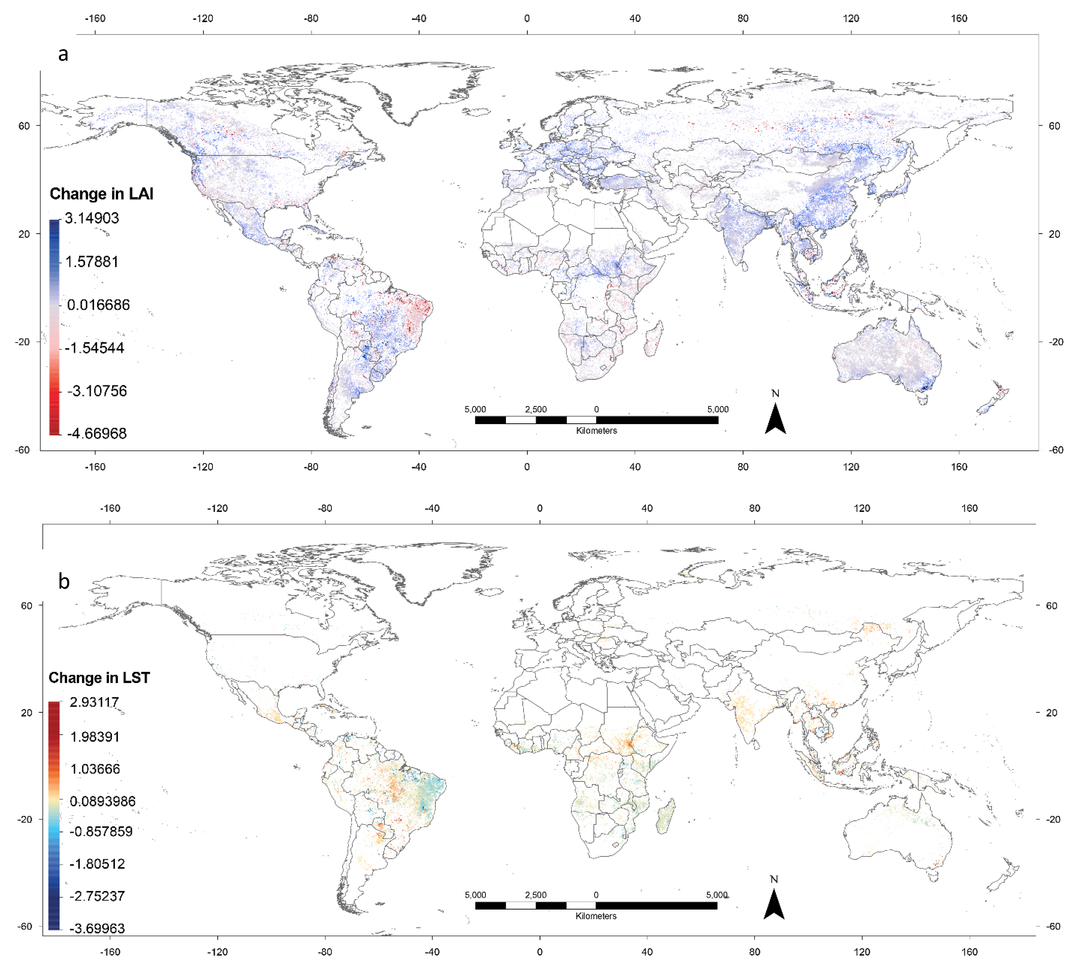
3.1.2. Change in Global LAI and LST during 2003 to 2018

Changes in mean LAI and LST between the reference (2003–2010) and experimental (2011–2018) periods were quantitatively analyzed through image differencing in order to investigate the spatiotemporal variations in vegetation and temperature dynamics (Figure 2a,b). Note that only the statistically significant changes (p < 0.05) are shown. Globally, the spatiotemporal variations of LAI with positive trends were more widespread than the negative trends during the study period (2003–2018). In fact, the areas with the most notable differences in LAI between the reference and experimental period (demonstrating an increasing trend), were in South and North America, Europe, Central Africa, Southeast and Southwest Asia, and Australia (Figure 2a). The observed LAI increases ranged between 0.016 and 3.149 m2/m2. LAI decreased in parts of North America, Africa, and the northeast of South America. This is demonstrated especially in South America by negative values (−4.669 to −1.545 m2/m2) over a large proportion of its vegetated surface since 2003. Changes in mean LST between the reference and experimental periods were very much insignificant across most of the globe (Figure 2b). Areas with increased LST were observed in central South America (the Amazon), some parts of Europe and Southwest Asia. During this period, the increase in LST ranged between 0.089 and 2.931, while negative changes ranged from −3.699 to −0.805 K, as seen in the Amazon and eastern Central Africa (Figure 2b).

3.2. Continental LAI and LST

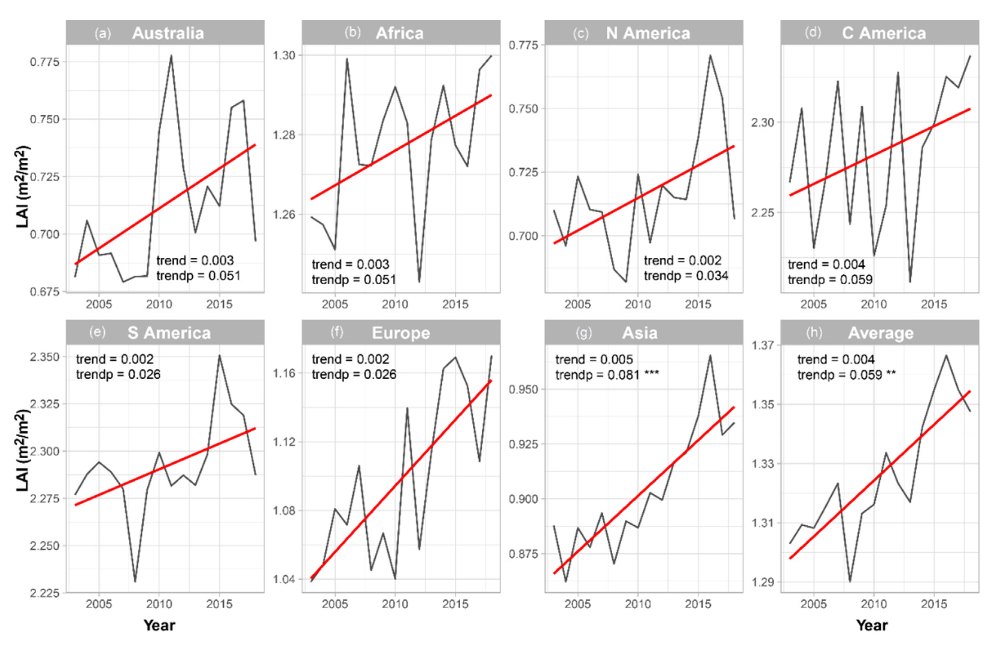
3.2.1. Trends of Continental LAI

The temporal pattern of trends in LAI for different continents is shown in Figure 3a–h. Both the annual trend and trend during the period (trendp) were estimated for each continent. In all cases, during the study period (2003–2018), all continents demonstrated a greening trend even though the rate of change in LAI varied. The year to year trend of LAI ranged between 0.002 and 0.005, while for the trend period it was 0.026 to 0.081. The Asian continent had the most significant trendp (0.081). Overall, the average LAI for all the continents exhibited a significant greening over the study period.

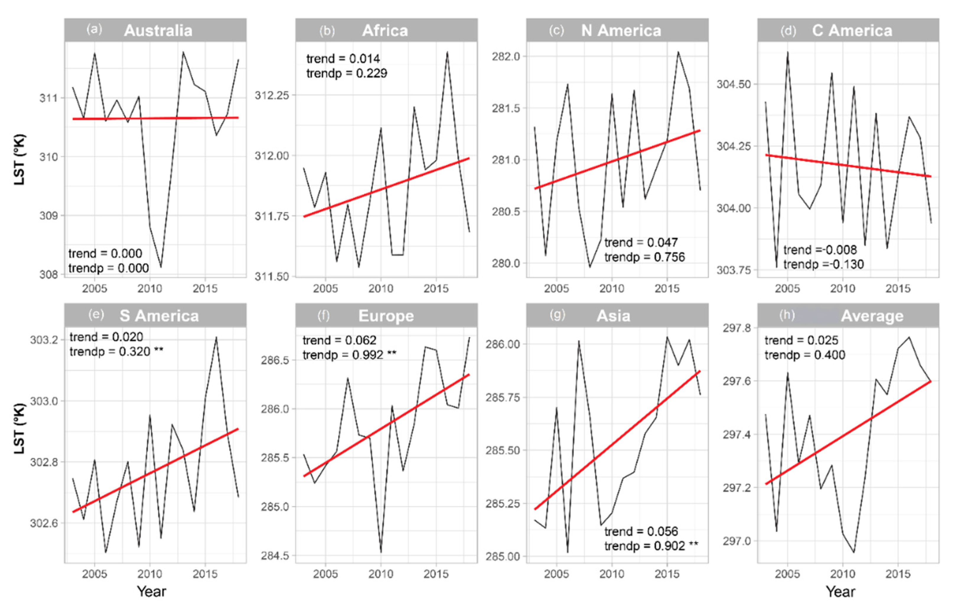
3.2.2. Trend of Continental LST

The temporal trends in LST for different continents can be seen in Figure 4a–h. Both trend and trendp were estimated for each continent. The changing trends of LST varied by continent. For example, in Australia, no trend was observed, however there was a very sharp drop in LST in 2010. In Africa (trendp = 0.229) and North America (trendp = 0.756), an increasing trend was observed. In contrast, a decreasing trend of LST was observed for Central America. Although the increasing trend of LST was greater in South America (trendp = 0.320) compared to Africa, Europe (trendp = 0.992) and Asia (trendp = 0.902) had the most significant increase in LST over the study period.

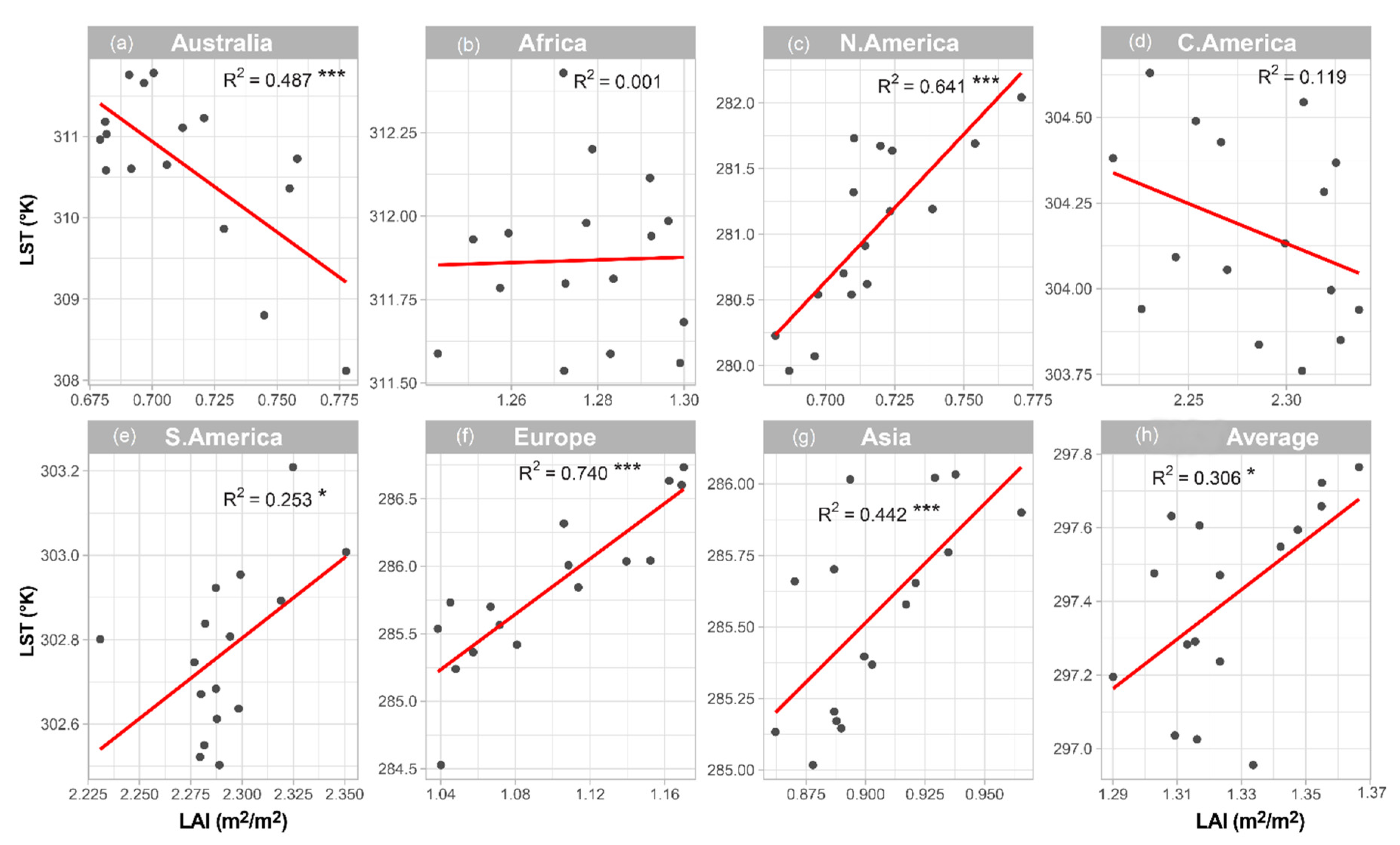
3.2.3. LAI and LST Continental Relationship

The relationship between LAI and LST was assessed for each continent to ascertain the response of vegetation to changes in LST (Figure 5a–h). In Australia, a moderate inverse relationship was observed between the LAI and LST (R2 = 0.487). No significant relationship was found in Africa (R2 = 0.001), while a strong/significant relationship was observed in North America’s LST (R2 = 0.641). This demonstrates high sensitivity of photosynthetic vegetation to LST on this continent. In Central America, a weak inverse relationship was found (R2 = 0.119). Again, a weak but significant relationship was observed for South America (R2 = 0.253). A strong positive relationship was observed in Europe (R2 = 0.740), and this was the most significant relationship compared with all the other continents. This may indicate that vegetation responds strongly to changes in LST in Europe. In Asia, a moderate positive relationship was observed (R2 = 0.442). The relationship between the average LAI and the LST for all continents showed a positive relationship (R2 = 0.306).

3.3. LAI and LST in the Most Greening Countries during 2003 to 2018

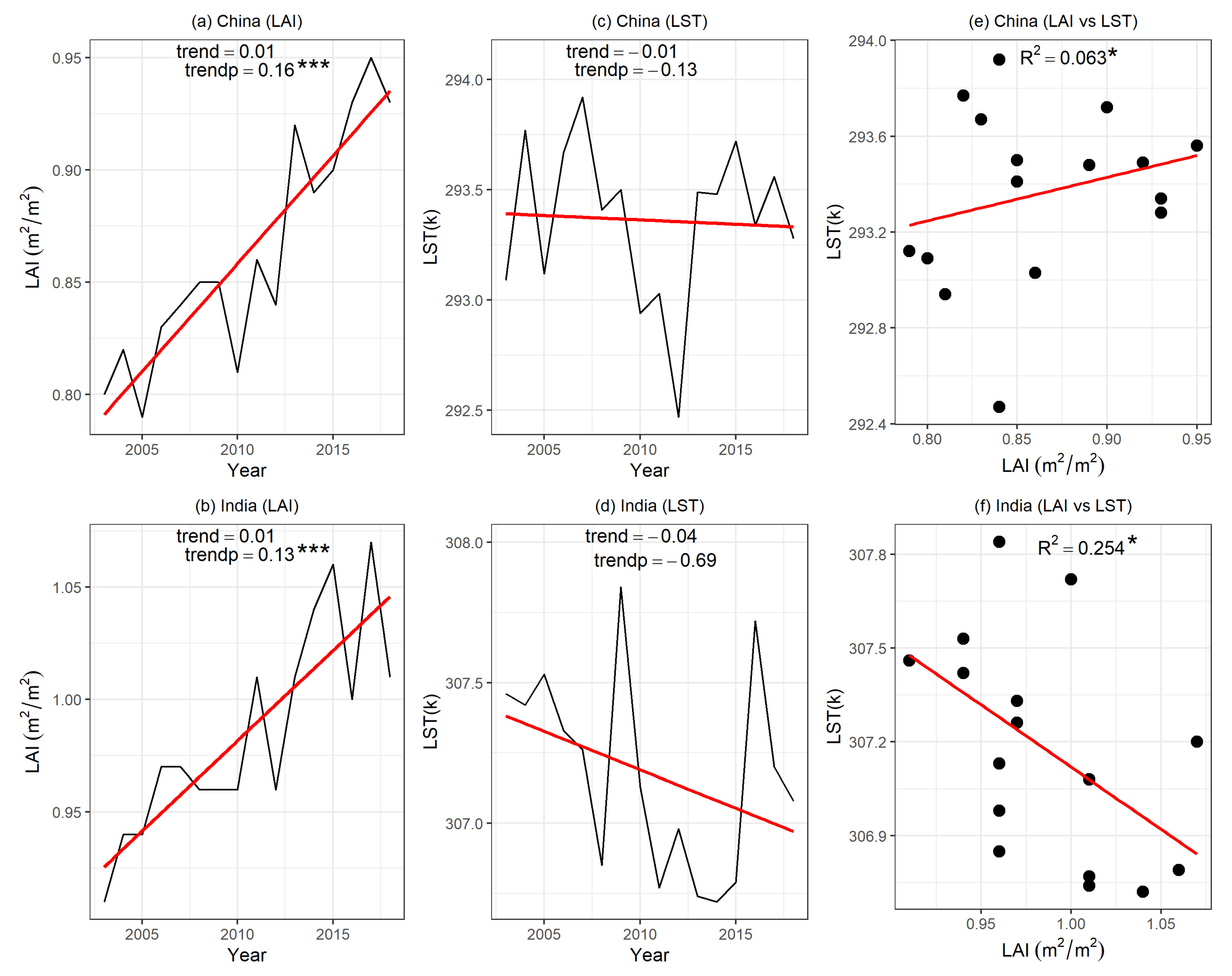
3.3.1. Trend of LAI and LST in China and India

Figure 6a–f demonstrates the trends of LAI and LST for China and India. The LAI for the two countries increased during 2003 to 2018. The trends exhibited significant positive change, with trendp = 0.16 *** and trendp = 0.13 *** for China and India, respectively (Figure 6b). However, the increase in the LAI is higher (0.79–0.935/LAI) in China (Figure 6a) than in India (0.925–1.05/LAI) (Figure 6b). The LST for the two also varied. In China, there was no significant trend (trendp = −0.13) in LST (Figure 6c). In India, there was a negative trend (trendp = −0.69) in LST (Figure 6d).

3.3.2. Relationship between LAI and LST in China and India

The relationships between the LAI and LST for two countries were assessed to ascertain if LAI responds to change in LST (Figure 6e,f). Despite the significant positive change in LAI over the study period in China, the relationship between the LAI and LST was not significant (R2 = 0.063). This is possibly due to there being no significant change in LST for this particular country over the study period. Conversely, although India showed a weak inverse relationship between the LST and LAI (R2 = 0.254), this relationship is stronger than what was found for China. This is because the country demonstrates a decreasing LST trend especially, from 2010 to 2015 (Figure 6d).

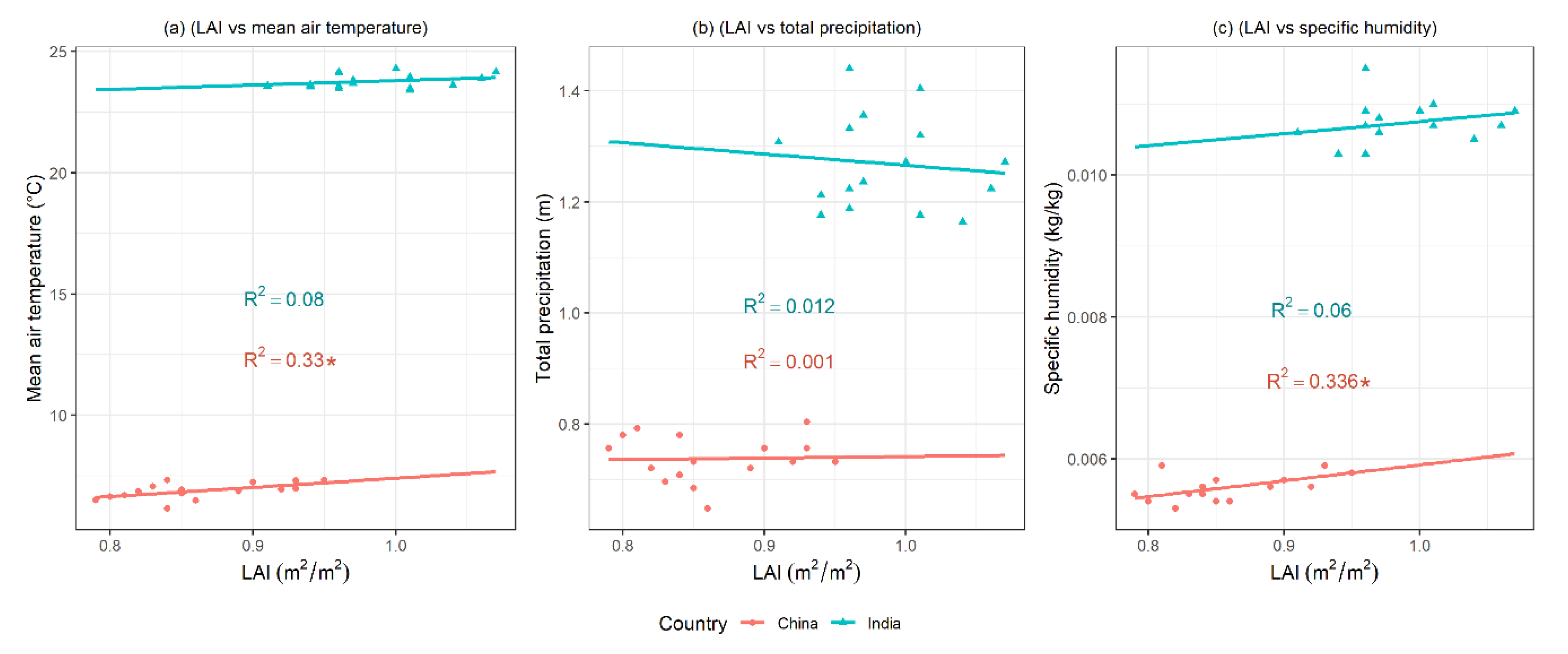
3.3.3. Relationship between LAI and Air Temperature, Humidity and Precipitation in China and India

The relationships between the LAI and air temperature, specific humidity, and total precipitation for China and India were assessed to determine if climatic variables are associated with changes in LAI (Figure 7a–c). Despite the significant positive change of LAI over the study period in India, the relationship between the LAI and selected climatic variables (mean air temperature, annual specific humidity, and the annual total precipitation) was not significant. In China, a weak positive relationship between LAI and air temperature (R2 = 0.33) and specific humidity (R2 = 0.336) was observed. The country displayed increasing air temperature and specific humidity in association with increasing LAI during the study period (Figure 7a,c). Meanwhile, no relationship was observed between total precipitation and LAI trend in both India and China (Figure 7b).

4. Discussion

This study examined the trend and linear regression modeling of level 4 LAI and LST derived from MODIS data, specifically to assess their spatial distribution and changing trends at the continental and regional scales. We employed a change-detection approach to quantify the interannual variability in the global LAI and LST between two periods (2003–2010 and 2011–2018). To address some of the peculiarities among regions, such as that of the most prominent greening countries in the world, the relationships between the LAI and LST over China and India were investigated. An investigation into the changing trends of LAI and LST, and their interannual variability at the regional and global levels, could reveal ecological processes and biosphere–atmosphere interactions, setting the basis for monitoring vegetation and climate feedback [12,19,28].
The current study highlights the spatial details of the changing global LAI and LST by mapping the spatial patterns of linear trends between two periods (2003–2010 and 2011–2018). Globally, the spatiotemporal variations in LAI demonstrate more positive trends than negative (Figure 2a). This is consistent with the findings of previous research that observed an increase in growing season integrated LAI (greening) from 25% to 50% of the global vegetated area during 1982–2009 [12]. In fact, the areas with notable differences in LAI between the reference period (2003–2010) and 2011–2018, showing an increasing trend, are in South and North America, Europe, Central Africa, and Southeast and Southwest Asia. However, Eurasia demonstrates a more subtle greening than North America [43]. Recent evidence suggests that some of these regions (e.g., China) have an increased greening trend [22], and historically, most of these regions have records of growing LAI [11,12,44]. This study found greening and browning trends of the global LAI in the ranges of 0.016 to 3.15 and −4.669 to −1.545, respectively. Conversely, changes in LST between 2003 and 2010 and 2011 and 2018 were very much insignificant across a large proportion of the globe (Figure 2b). Areas with positive increases in LST were observed in Central America, the Amazon, some parts of Europe and Southwest Asia. The increases and decreases in LST ranged from 0.089 to 2.931 and −3.699 to −0.805 K, respectively.
To understand the spatial pattern of the global LAI and LST more effectively, we assessed their temporal trends and relationships per continent. The trend of the LAI and LST varied by continent. In general, all continents demonstrate a greening trend. The most significant greening trend (trendp = 0.081) was found in Asia. This can be explained by the increase in land use management activities (e.g., agriculture) in this part of the world [22]. For the LST, the most significant trends were found in South America, Europe and Asia. The relationship between the LAI and LST further indicates how differences in LST within continents affect the LAI trend. The strong inverse relationship between the LAI and the LST in Australia (Figure 5), and the absence of trend in Africa, are likely due to the increasing anthropogenic activities (e.g., fires, deforestation, drought, etc.) and high interannual variability [45,46,47]. In contrast, LAI and LST in North America (R2 = 0.64 ***), Europe (R2 = 0.4 ***), and Asia (R2 = 0.64 ***) have indicated significant relationships (Figure 5). The socio-economic and biophysical characteristics of these regions differ compared to other regions, such as medium temperature in Europe, which enhances plants’ photosynthetic activities. Zhu et al. [12] and Zhu et al. [12] disclosed that in the northern high latitudes, rising temperatures, which enhance photosynthesis and lengthen the growing season, are the dominant climatic factor contributing to greening trends. In Asia, for example, increased agricultural activities in countries such as China and India contribute substantially to greening trends. The conversion of the relationship between LST and LAI from positive to inverse in different regions could be attributed to decreasing photosynthesis when the temperature exceeds the temperature optimum of photosynthesis (20 to 30 °C) [48,49].
From our results, we observed a significant greening trend, with trendp = 0.16 *** and trendp = 0.13 *** (Figure 6a,b) for China and India, respectively. These results together confirmed the findings of a recent study by Chen et al. (2019), despite a slight difference in the temporal observations of the satellite data assessed by the two studies. However, this study found an insignificant LST trend, R2 = 0.002, for China (Figure 6c), and a weak negative trend (R2 = 0.13) for India (Figure 6d). In addition to quantifying the relationship between the LAI and LST in these countries, this study also provides an important insight into how the vegetation dynamics in these greening parts of the globe affect the LST derived from data from a 16-year MODIS time series. Since the photosynthesis of vegetation requires an optimum temperature, changes in temperature also affect vegetation dynamics. An insignificant relationship was found between LAI and LST in China. In contrast to the relationship observed in India, a weak inverse (R2 = 0.24) was observed. A recent study by Yu et al. [50] studied the impact of recent vegetation greening on temperature and precipitation over China. The study found a surface cooling of 0.11 °C and a precipitation increase of 0.02 mm/d during summer in response to China’s widespread greening. The study assessed the regional variability of climatic responses to greening. Northern China showed significant cooling, while no significant temperature changes were observed in southern China. They discussed that vegetation greening is influencing the occurrence of extreme climate events by decreasing the number of heatwave days (by 1–3 days, particularly in northern China), reducing drought events in northern China, and minimizing the risk of floods in southern China.
The differences between China and India, in terms of their changes in LAI and the relationship between LAI and LST, could be due to the differences in the nature of land use/cover (e.g., forest or cropland) that were to found to contribute substantially to the greening of these two countries. This is because the feedback of vegetation to climate ais mediated by phenology, which is largely influenced by factors such as albedo, surface roughness and canopy conductance [25]. China accounts for 25% of the global net increase in leaf area, and a large proportion of the contribution comes from forests (42%) and croplands (32%). This assists us in stabilizing the climate by lowering the temperature (Yu et al. [50]), while in India, the greening is mostly from the croplands (82%), and only a negligible proportion is from forests (4.4%) [22]. The phenomenon of an increase in LAI leading to decreasing LST in India can be explained based on the influence of all the factors mentioned above, but of particular importance is the surface roughness length. Richardson et al. [25] disclosed that increases in surface roughness length are associated with an increase in the efficiency with which sensible heat is transferred from the surface, but surface roughness length varies according to seasonal changes in canopy structure. In agricultural crops, surface roughness increases substantially over the course of the growing season, as there is transition from bare ground to tall plants. In India, the greening trend was high from 2011 to 2018. The poor relationship between the LAI and precipitation may be due to the influence of ecosystem management practices in China and India [12]. We attribute these changes in greening to land use management and the climate mitigation options adopted by these countries.

5. Conclusions

This study presented the trends of and linear regression modeling for level 4 LAI and LST derived from MODIS data, specifically to assess their spatial distribution and their changing trends at the continental and regional scales. For example, China and India were determined as the most greening parts of the globe. The following conclusions can be drawn:
  • The current study highlights the spatial details of the changing global LAI and LST by mapping the spatial patterns of linear trends between two periods (2003–2010 and 2011–2018). Globally, the spatiotemporal variations in LAI between both periods demonstrate more positive trends than negative;
  • The continental patterns of LAI and LST trends, and their linear relationships, indicated that LAI and LST varied by continent. In general, during the study period (2003–2018), all continents demonstrated a greening trend, with the most significant greening trend (trendp = 0.081) in Asia. The relationships between the LAI and LST in North America (R2 = 0.64 ***), Europe (R2 = 0.4 ***) and Asia (R2 = 0.64 ***) were very significant;
  • We observed a significant greening trend for China and India, respectively (trendp = 0.16 *** and trendp = 0.13 ***), from 2003 to 2018. These results together confirmed the results presented by Chen et al. [22], despite a slight difference in the temporal observations of the satellite data product assessed by the two studies. Besides this, the study also found an insignificant LST trend for China (trendp = –0.13) and a weak negative trend for India (trendp = –0.69).
  • An insignificant relationship between the LAI and LST in China (R2 = 0.057) is indicative of the impact of the positive greening trend on LAI. In contrast, a weak inverse relationship (R2 = 0.24) was observed for India and is attributed to a strong positive change in LAI in recent times, in this particular country, as observed in this study.
  • A weak positive relationship between LAI and mean air temperature and specific humidity was observed in China. However, no relationship was found between LAI and selected climatic variables in India.

Author Contributions

Conceptualization, A.R.; Data curation, A.R.; Formal analysis, S.I. and A.R.; Investigation, A.R.; Methodology, A.R.; Visualization, A.R. and A.R.O.; Writing—original draft, A.R., S.I. and H.B.; Writing—review and editing, A.R., S.I., A.R.O. and H.B. All authors have read and agreed to the published version of the manuscript.

Funding

This research is supported by the National Centre for Earth Observation (NERC).

Conflicts of Interest

The authors declare no conflict of interest.

Appendix A

Table A1. Continental LAI from 2003 to 2018 that was extracted from the MODIS 006/MCD15A3H product.
YearAustraliaAfricaN. AmericaC. AmericaS. AmericaEuropeAsiaContinental Average
20030.6641.2130.7792.2572.3500.9601.1051.333
20040.6911.2100.7682.3002.3610.9731.0891.342
20050.6731.2050.8012.2232.3691.0091.1041.341
20060.6771.2490.7842.2612.3620.9851.1091.347
20070.6641.2270.7852.3142.3541.0241.1171.355
20080.6661.2220.7612.2352.3020.9651.0921.321
20090.6661.2360.7512.3002.3560.9881.1141.344
20100.7291.2450.8002.2182.3740.9811.1181.352
20110.7621.2350.7692.2452.3561.0551.1221.363
20120.7121.1970.7912.3192.3610.9951.1041.354
20130.6841.2340.7822.2032.3541.0351.1401.347
20140.7041.2450.7852.2772.3701.0711.1511.372
20150.6951.2340.8142.2922.4261.0641.1681.385
20160.7381.2280.8462.3162.3971.0841.1781.398
20170.7421.2490.8282.3112.3921.0201.1521.385
20180.6811.2520.7792.3292.3581.0791.1611.377
Table A2. Continental LST from 2003 to 2018 that was extracted from the Aqua daytime 006/MYD11A2 product.
YearAustraliaAfricaN. AmericaC. AmericaS. AmericaEuropeAsiaContinental Average
2003311.55311.38284.29304.45302.98283.56295.42299.09
2004311.00311.30283.13303.77302.82283.28295.57298.69
2005312.13311.38284.17304.64303.04283.85295.76299.28
2006310.91311.07284.71304.08302.72283.34295.41298.89
2007311.29311.26283.56304.01302.92284.45295.98299.07
2008310.93311.01283.05304.11302.99283.89295.71298.81
2009311.37311.25283.21304.56302.73283.71295.56298.91
2010309.13311.60284.43303.96303.20283.25295.64298.74
2011308.42311.07283.60304.52302.75283.99295.49298.55
2012310.20311.01284.86303.88303.15283.80295.46298.91
2013312.14311.65283.60304.40303.04284.03295.74299.23
2014311.56311.39283.80303.86302.88284.41295.85299.11
2015311.46311.43284.09304.14303.26284.56296.06299.29
2016310.73311.93284.88304.39303.46284.34296.04299.39
2017311.06311.50284.61304.31303.14284.35296.10299.30
2018312.00311.21283.68303.96302.91284.50295.82299.15
Table A3. LAI and LST of China and India from 2003 to 2018 that was extracted from the MODIS 006/MCD15A3H and Aqua daytime 006/MYD11A2 products.
YearLAI (China)LST (China)LAI (India)LST (India)
20030.80293.090.91307.46
20040.82293.770.94307.42
20050.79293.120.94307.53
20060.83293.670.97307.33
20070.84293.920.97307.26
20080.85293.410.96306.85
20090.85293.500.96307.84
20100.81292.940.96307.13
20110.86293.031.01306.77
20120.84292.470.96306.98
20130.92293.491.01306.74
20140.89293.481.04306.72
20150.90293.721.06306.79
20160.93293.341.00307.72
20170.95293.561.07307.20
20180.93293.281.01307.08

References

  1. Asner, G.P.; Martin, R.E. Airborne spectranomics: Mapping canopy chemical and taxonomic diversity in tropical forests. Front. Ecol. Environ. 2009, 7, 269–276. [Google Scholar] [CrossRef] [Green Version]
  2. Deng, F.; Chen, J.M.; Plummer, S.; Chen, M.; Pisek, J. Algorithm for global leaf area index retrieval using satellite imagery. IEEE Trans. Geosci. Remote Sens. 2006, 44, 2219–2229. [Google Scholar] [CrossRef] [Green Version]
  3. Xiao, Z.; Liang, S.; Wang, J.; Xiang, Y.; Zhao, X.; Song, J. Long-time-series global land surface satellite leaf area index product derived from MODIS and AVHRR surface reflectance. IEEE Trans. Geosci. Remote Sens. 2016, 54, 5301–5318. [Google Scholar] [CrossRef]
  4. Liu, Y.; Liu, R.; Chen, J.M. Retrospective retrieval of long-term consistent global leaf area index (1981–2011) from combined AVHRR and MODIS data. J. Geophys. Res. Biogeosci. 2012, 117. [Google Scholar] [CrossRef]
  5. Zhu, Z.; Bi, J.; Pan, Y.; Ganguly, S.; Anav, A.; Xu, L.; Samanta, A.; Piao, S.; Nemani, R.R.; Myneni, R.B. Global data sets of vegetation leaf area index (LAI) 3g and fraction of photosynthetically active radiation (FPAR) 3g derived from global inventory modeling and mapping studies (GIMMS) normalized difference vegetation index (NDVI3g) for the period 1981 to 2011. Remote Sens. 2013, 5, 927–948. [Google Scholar]
  6. Tum, M.; Günther, K.P.; Böttcher, M.; Baret, F.; Bittner, M.; Brockmann, C.; Weiss, M. Global gap-free MERIS LAI time series (2002–2012). Remote Sens. 2016, 8, 69. [Google Scholar] [CrossRef] [Green Version]
  7. Shabanov, N.V.; Huang, D.; Yang, W.; Tan, B.; Knyazikhin, Y.; Myneni, R.B.; Ahl, D.E.; Gower, S.T.; Huete, A.R.; Aragão, L.E.O. Analysis and optimization of the MODIS leaf area index algorithm retrievals over broadleaf forests. IEEE Trans. Geosci. Remote Sens. 2005, 43, 1855–1865. [Google Scholar] [CrossRef] [Green Version]
  8. Yan, K.; Park, T.; Yan, G.; Chen, C.; Yang, B.; Liu, Z.; Nemani, R.R.; Knyazikhin, Y.; Myneni, R.B. Evaluation of MODIS LAI/FPAR product collection 6. Part 1: Consistency and improvements. Remote Sens. 2016, 8, 359. [Google Scholar] [CrossRef] [Green Version]
  9. Buermann, W.; Dong, J.; Zeng, X.; Myneni, R.B.; Dickinson, R.E. Evaluation of the utility of satellite-based vegetation leaf area index data for climate simulations. J. Clim. 2001, 14, 3536–3550. [Google Scholar] [CrossRef]
  10. Myneni, R.B.; Yang, W.; Nemani, R.R.; Huete, A.R.; Dickinson, R.E.; Knyazikhin, Y.; Didan, K.; Fu, R.; Juárez, R.I.N.; Saatchi, S.S. Large seasonal swings in leaf area of Amazon rainforests. Proc. Natl. Acad. Sci. USA 2007, 104, 4820–4823. [Google Scholar] [CrossRef] [Green Version]
  11. Piao, S.; Yin, G.; Tan, J.; Cheng, L.; Huang, M.; Li, Y.; Liu, R.; Mao, J.; Myneni, R.B.; Peng, S. Detection and attribution of vegetation greening trend in China over the last 30 years. Glob. Chang. Biol. 2015, 21, 1601–1609. [Google Scholar] [CrossRef] [PubMed]
  12. Zhu, Z.; Piao, S.; Myneni, R.B.; Huang, M.; Zeng, Z.; Canadell, J.G.; Ciais, P.; Sitch, S.; Friedlingstein, P.; Arneth, A.; et al. Greening of the Earth and its drivers. Nat. Clim. Chang. 2016, 6, 791–795. [Google Scholar] [CrossRef]
  13. Chen, J.M.; Black, T.A. Defining leaf area index for non-flat leaves. Plant Cell Environ. 1992, 15, 421–429. [Google Scholar] [CrossRef]
  14. Global Climate Observing System. Available online: https://public.wmo.int/en/programmes/global-climate-observing-system (accessed on 27 August 2020).
  15. Yan, H.; Wang, S.Q.; Billesbach, D.; Oechel, W.; Zhang, J.H.; Meyers, T.; Martin, T.A.; Matamala, R.; Baldocchi, D.; Bohrer, G. Global estimation of evapotranspiration using a leaf area index-based surface energy and water balance model. Remote Sens. Environ. 2012, 124, 581–595. [Google Scholar] [CrossRef] [Green Version]
  16. Gower, S.T.; Kucharik, C.J.; Norman, J.M. Direct and indirect estimation of leaf area index, fAPAR, and net primary production of terrestrial ecosystems. Remote Sens. Environ. 1999, 70, 29–51. [Google Scholar] [CrossRef]
  17. Jonckheere, I.; Fleck, S.; Nackaerts, K.; Muys, B.; Coppin, P.; Weiss, M.; Baret, F. Review of methods for in situ leaf area index determination: Part I. Theories, sensors and hemispherical photography. Agric. For. Meteorol. 2004, 121, 19–35. [Google Scholar] [CrossRef]
  18. Asner, G.P.; Scurlock, J.M.; Hicke, J.A. Global synthesis of leaf area index observations: Implications for ecological and remote sensing studies. Glob. Ecol. Biogeogr. 2003, 12, 191–205. [Google Scholar] [CrossRef] [Green Version]
  19. Turner, D.P.; Cohen, W.B.; Kennedy, R.E.; Fassnacht, K.S.; Briggs, J.M. Relationships between leaf area index, fapar, and net primary production of terrestrial ecosystems. Remote Sens. Environ. 1999, 70, 52–68. [Google Scholar] [CrossRef]
  20. Munier, S.; Carrer, D.; Planque, C.; Camacho, F.; Albergel, C.; Calvet, J.-C. Satellite Leaf Area Index: Global scale analysis of the tendencies per vegetation type over the last 17 years. Remote Sens. 2018, 10, 424. [Google Scholar] [CrossRef] [Green Version]
  21. Pan, N.; Feng, X.; Fu, B.; Wang, S.; Ji, F.; Pan, S. Increasing global vegetation browning hidden in overall vegetation greening: Insights from time-varying trends. Remote Sens. Environ. 2018, 214, 59–72. [Google Scholar] [CrossRef]
  22. Chen, C.; Park, T.; Wang, X.; Piao, S.; Xu, B.; Chaturvedi, R.K.; Fuchs, R.; Brovkin, V.; Ciais, P.; Fensholt, R. China and India lead in greening of the world through land-use management. Nat. Sustain. 2019, 2, 122–129. [Google Scholar] [CrossRef] [PubMed]
  23. Huang, M.; Piao, S.; Ciais, P.; Peñuelas, J.; Wang, X.; Keenan, T.F.; Peng, S.; Berry, J.A.; Wang, K.; Mao, J. Air temperature optima of vegetation productivity across global biomes. Nat. Ecol. Evol. 2019, 3, 772–779. [Google Scholar] [CrossRef]
  24. Peñuelas, J.; Filella, I. Phenology feedbacks on climate change. Science 2009, 324, 887–888. [Google Scholar] [CrossRef] [PubMed] [Green Version]
  25. Richardson, A.D.; Keenan, T.F.; Migliavacca, M.; Ryu, Y.; Sonnentag, O.; Toomey, M. Climate change, phenology, and phenological control of vegetation feedbacks to the climate system. Agric. For. Meteorol. 2013, 169, 156–173. [Google Scholar] [CrossRef]
  26. Cowles, J.; Boldgiv, B.; Liancourt, P.; Petraitis, P.S.; Casper, B.B. Effects of increased temperature on plant communities depend on landscape location and precipitation. Ecol. Evol. 2018, 8, 5267–5278. [Google Scholar] [CrossRef] [PubMed]
  27. Peng, S.-S.; Piao, S.; Zeng, Z.; Ciais, P.; Zhou, L.; Li, L.Z.; Myneni, R.B.; Yin, Y.; Zeng, H. Afforestation in China cools local land surface temperature. Proc. Natl. Acad. Sci. USA 2014, 111, 2915–2919. [Google Scholar] [CrossRef] [Green Version]
  28. Tao, F.; Chen, Y.; Fu, B. Impacts of climate and vegetation leaf area index changes on global terrestrial water storage from 2002 to 2016. Sci. Total Environ. 2020, 724, 138298. [Google Scholar] [CrossRef]
  29. modis.gsfc.nasa.gov MODIS. Available online: https://modis.gsfc.nasa.gov/about/ (accessed on 12 September 2020).
  30. Wan, Z.; Hook, S.; Hulley, G. MYD11A2 MODIS/Aqua Land Surface Temperature/Emissivity 8-Day L3 Global 1km SIN Grid V006. Available online: https://doi.org/10.5067/MODIS/MYD11A2.006 (accessed on 12 September 2020).
  31. Myneni, Y.K.R. MCD15A3H MODIS/Terra+Aqua Leaf Area Index/FPAR 4-day L4 Global 500m SIN Grid V006; LP DAAC: Sioux Falls, SD, USA, 2015. [Google Scholar] [CrossRef]
  32. Saha, S.; Moorthi, S.; Wu, X.; Wang, J.; Nadiga, S.; Tripp, P.; Behringer, D.; Hou, Y.T.; Chuang, H.-Y.; Iredell, M. NCEP climate forecast system version 2 (CFSv2) 6-hourly products. In Research Data Archive at the National Center for Atmospheric Research, Computational and Information Systems Laboratory; NCEP: Boulder, CO, USA, 2011. [Google Scholar] [CrossRef]
  33. ECMWF. Copernicus Climate Change Service (C3S) ERA5: Fifth generation of ECMWF atmospheric reanalyses of the global climate. In Copernicus Climate Change Service Climate Data Store (CDS); ECMWF: Reading, UK, 2017. [Google Scholar]
  34. Gorelick, N.; Hancher, M.; Dixon, M.; Ilyushchenko, S.; Thau, D.; Moore, R. Google Earth Engine: Planetary-scale geospatial analysis for everyone. Remote Sens. Environ. 2017, 202, 18–27. [Google Scholar] [CrossRef]
  35. Team, R.C. R: A Language And Environment for Statistical Computing; The R Foundation for Statistical Computing: Vienna, Austria, 2020. [Google Scholar]
  36. Wickham, H.; Francois, R.; Henry, L.; Müller, K. dplyr: A Grammar of Data Manipulation. R package version 0.4. 3. The R Foundation for Statistical Computing, Vienna. 2015. Available online: https://CRAN.R-project.org/package=dplyr (accessed on 12 October 2020).
  37. Wickham, H. The Tidyverse. R package ver. 2017. Available online: https://slides.nyhackr.org/presentations/The-Tidyverse_Hadley-Wickham.pdf (accessed on 12 October 2020).
  38. Kassambara, A. Package “ggpubr”.’ggplot2’ Based Publication Ready Plots Version. 2020. Available online: https://CRAN.R-project.org/package=clinfun (accessed on 12 October 2020).
  39. Wickham, H.; Chang, W.; Wickham, M.H. Package ‘ggplot2.’ Create Elegant Data Visualisations Using the Grammar of Graphics Version. 2020. Available online: https://ggplot2.tidyverse.org/reference/ggplot2-package.html (accessed on 12 October 2020).
  40. Bronaugh, D.; Werner, A.; Bronaugh, M.D. Package ‘zyp.’ CRAN Repository. 2009. Available online: https://cran.biodisk.org/web/packages/zyp/zyp.pdf (accessed on 12 October 2020).
  41. Carslaw, D.C. Section 15 Theil-Sen Trends | The Openair Book. Available online: https://bookdown.org/david_carslaw/openair/sec-TheilSen.html (accessed on 12 October 2020).
  42. Yue, S.; Pilon, P.; Cavadias, G. Power of the Mann–Kendall and Spearman’s rho tests for detecting monotonic trends in hydrological series. J. Hydrol. 2002, 259, 254–271. [Google Scholar] [CrossRef]
  43. Yan, K.; Park, T.; Chen, C.; Xu, B.; Song, W.; Yang, B.; Zeng, Y.; Liu, Z.; Yan, G.; Knyazikhin, Y. Generating global products of lai and fpar from snpp-viirs data: Theoretical background and implementation. IEEE Trans. Geosci. Remote Sens. 2018, 56, 2119–2137. [Google Scholar] [CrossRef]
  44. Jiang, C.; Ryu, Y.; Fang, H.; Myneni, R.; Claverie, M.; Zhu, Z. Inconsistencies of interannual variability and trends in long-term satellite leaf area index products. Glob. Chang. Biol. 2017, 23, 4133–4146. [Google Scholar] [CrossRef] [PubMed]
  45. Valentini, R.; Arneth, A.; Bombelli, A.; Castaldi, S.; Cazzolla Gatti, R.; Chevallier, F.; Ciais, P.; Grieco, E.; Hartmann, J.; Henry, M. A full greenhouse gases budget of Africa: Synthesis, uncertainties, and vulnerabilities. Biogeosciences 2014, 11, 381–407. [Google Scholar] [CrossRef] [Green Version]
  46. Bombelli, A.; Henry, M.; Castaldi, S.; Adu-Bredu, S.; Arneth, A.; De Grandcourt, A.; Grieco, E.; Kutsch, W.L.; Lehsten, V.; Rasile, A. An outlook on the Sub-Saharan Africa carbon balance. Biogeosciences 2009, 6, 2193–2205. [Google Scholar] [CrossRef] [Green Version]
  47. Jiao, T.; Williams, C.A.; Rogan, J.; De Kauwe, M.G.; Medlyn, B.E. Drought impacts on australian vegetation during the millennium drought measured with multisource spaceborne remote sensing. J. Geophys. Res. Biogeosciences 2020, 125, e2019JG005145. [Google Scholar] [CrossRef]
  48. Wardlaw, I.F. Temperature control of translocation. In Mechanism of Regulation of Plant Growth; Bielske, R.L., Ferguson, A.R., Cresswell, M.M., Eds.; Bull. Royal Soc.: Wellington, New Zealand, 1974; pp. 533–538. [Google Scholar]
  49. Abrol, Y.P.; Ingram, K.T. Effects of higher day and night temperatures on growth and yields of some crop plants. In Global Climate Change and Agricultural Production: Direct and Indirect Effects of Changing Hydrological, Pedological and Plant Physiological Processes; Wiley: Chichester, UK, 1996; pp. 124–140. [Google Scholar]
  50. Yu, L.; Liu, Y.; Liu, T.; Yan, F. Impact of recent vegetation greening on temperature and precipitation over China. Agric. For. Meteorol. 2020, 295, 108197. [Google Scholar] [CrossRef]
Figure 1. (a) Mean leaf area index (LAI) and (b) mean land surface temperature (LST) during 2018.
Land 09 00388 g001
Figure 2. (a) Difference between mean LAI of 2003–2010 and 2011–2018, and (b) mean LST of 2003–2010 and 2011–2018 in kelvin. Insignificant changes (p > 0.05) have been masked out.
Land 09 00388 g002
Figure 3. Trend of continental LAI from 2003 to 2018. ***: p < 0.001, **: p < 0.01.
Land 09 00388 g003
Figure 4. Trend of continental LST from 2003 to 2018. **: p < 0.01.
Land 09 00388 g004
Figure 5. Continental relationship between LAI and LST from 2003 to 2018. ***: p < 0.001, *: p < 0.05.
Land 09 00388 g005
Figure 6. (af): Trend of LAI and LST in China and India, and relationship between them, from 2003 to 2018. ***: p < 0.001, *: p < 0.05.
Land 09 00388 g006
Figure 7. Relationship between LAI and annual mean air temperature (a), specific humidity (b) and total precipitation (c) in China and India from 2003 to 2018. *: p < 0.05.
Land 09 00388 g007
Table 1. Details of the data used in the research from 2003 to 2018.
DataTemporal ResolutionSpatial ResolutionData ID in GEESelected Band
Daytime Land Surface Temperature (Aqua)8 days1 kmMODIS/006/MYD11A2LST_Day_1km
Leaf Area Index 4 days 500 mMODIS/006/MCD15A3HLai
Air temperatureMonthly0.25 arc degreesECMWF/ERA5/MONTHLYmean_2m_air_temperature
Total precipitationMonthly0.25 arc degreesECMWF/ERA5/MONTHLYtotal_precipitation
Specific humidityFour times per day0.2 arc degreesNOAA/CFSV2/FOR6HSpecific_humidity_height_above_ground

