Abstract
Northern Botswana is influenced by various socio-ecological drivers of landscape change. The African elephant (Loxodonta africana) is one of the leading sources of landscape shifts in this region. Developing the ability to assess elephant impacts on savanna vegetation is important to promote effective management strategies. The Moving Standard Deviation Index (MSDI) applies a standard deviation calculation to remote sensing imagery to assess degradation of vegetation. Used previously for assessing impacts of livestock on rangelands, we evaluate the ability of the MSDI to detect elephant-modified vegetation along the Chobe riverfront in Botswana, a heavily elephant-impacted landscape. At broad scales, MSDI values are positively related to elephant utilization. At finer scales, using data from 257 sites along the riverfront, MSDI values show a consistent negative relationship with intensity of elephant utilization. We suggest that these differences are due to varying effects of elephants across scales. Elephant utilization of vegetation may increase heterogeneity across the landscape, but decrease it within heavily used patches, resulting in the observed MSDI pattern of divergent trends at different scales. While significant, the low explanatory power of the relationship between the MSDI and elephant utilization suggests the MSDI may have limited use for regional monitoring of elephant impacts.
1. Introduction
Savanna ecosystems cover approximately one-fifth of the Earth’s land surface, extending from tropical to semi-arid regions [1,2]. Such areas are characterized by a continuous herbaceous layer with intermittent trees and/or shrubs [3]. This broad definition covers everything from areas of almost continuous woody cover to areas that are mostly grassland with a few sparse trees [1,4]. In light of this variability, savannas are typically defined by the complex interactions between tree and grass layers [1]. These interactions play an important role in the functioning of savannas by regulating nutrient cycling and resource availability, influencing the biomass and diversity of organisms the savanna can support [5,6]. In addition to extensive plant and animal populations, savannas are home to an increasing proportion of the world’s human population as well as the majority of its rangeland and livestock [1]. They are also among the ecosystems predicted to be the most sensitive to climate change [7], raising concerns about compounding effects of recent increases in the prevalence of droughts, crop failure, and water scarcity [8].
Savannas are the dominant land cover type in Africa, covering over half the continent [1,2]. While the abiotic template of rainfall, fire, and soil nutrients sets the broad patterns for savanna dynamics and diversity in Africa [9,10,11,12], biotic influences of humans and wildlife may also strongly influence savanna patterns and processes [3,13,14]. At local scales, herbivory and fire can have as large an effect on savanna dynamics as climate [3,15]. Elephants (Loxodonta africana) have received some of the greatest attention for their ability to influence savanna dynamics due to their large size and conspicuous effects on vegetation [16,17,18,19,20]. As a keystone species, elephants exert an impact on the environment disproportionate to their abundance [21]. They can cause direct mortality of trees when foraging and may increase susceptibility of trees to fire and frost [22]. Furthermore, elephants may reduce seedling recruitment and promote grass production where trees are removed, as well as altering vegetation structure and nutrient cycling [22,23,24]. Many of these processes play a beneficial role in savannas, making elephants an important part of a healthy ecosystem.
A recent report from a collaboration of international agencies stresses the dire threat to elephant populations in many parts of sub-Saharan Africa due to poaching, with populations in Central and West Africa facing possible elimination [25]. Poaching levels in southern Africa, however, have been lower than the rest of Africa and elephant populations in many areas have increased steadily since the early 1900s [25]. Ironically, there have been concerns raised in southern and East Africa about the negative impacts high elephant densities may have on vegetation and other herbivores, the so-called “elephant problem” [26,27,28].
Southern Africa is home to the world’s largest population of African elephants [29]. These animals serve as the basis for a booming tourism industry, generating jobs and revenue for local communities [30]. However, they are also a source of human-wildlife conflict, raiding crops and killing people and livestock [31,32,33]. In addition, modification of vegetation structure by elephants may affect other wildlife species positively or negatively, with ramifications for ecosystem sustainability. In systems where elephants promote open savannas, grazers are likely to benefit from increased food availability. For example, buffalo (Syncerus caffer) appear to prefer grazing in areas recently utilized by elephants in Tanzania and Botswana [34,35]. In Kenya’s Tsavo National Park, dramatic reductions in elephant numbers due to poaching led to increasing tree cover and a reduction in grazers such as kongoni (Acelaphus buselaphus), oryx (Oryx beisa), and zebra (Equus quagga) [36]. While opening of habitats by elephants may benefit grazers, some browser species are likely to be negatively impacted. Bushbuck (Tragelaphus scriptus) depend on thick cover and the bushbuck population in Chobe National Park, Botswana, declined between the 1960s and 1990s as increases in elephants led to a more open habitat [37]. Similarly, both lesser kudu (Tragelaphus imberbis) and bushbuck were eliminated from Amboseli National Park in Kenya as a result of vegetation changes caused by elephants [38]. Some mixed-feeders, however, like impala (Aepyceros melampus) and greater kudu (Tragelaphus strepsiceros) preferentially browse trees with accumulated elephant impact in Chobe National Park [39,40]. Similarly, impala and steinbuck (Raphicerus campestris) preferentially utilize elephant-impacted habitat in Hwange National Park, Zimbabwe [41]. Managers in elephant-dominated areas need information about the distribution of elephant impacts so that effective management decisions can be made which balance the needs of various wildlife species. Remote sensing indices offer the potential to provide these types of information.
The Moving Standard Deviation Index (MSDI) is a moving standard deviation filter applied to remotely sensed images to assess degradation [42]. Processes increasing soil heterogeneity can lead to habitat degradation in semi-arid systems [43]. By expressing the variability in vegetation and soil, the MSDI is used to indicate levels of habitat degradation. Validation studies in semi-arid rangelands of both South Africa and Australia show that areas with higher MSDI values exhibit increased degradation [42,44]. This spectral-based degradation assessment technique is an ideal application of remotely sensed data in semi-arid landscapes as it provides continuous and repeatable measures of patterns across the study area and has been shown to operate well in complex regions [42,45].
The MSDI is traditionally applied in a 3 × 3-pixel moving window to the red band of remote sensing imagery [42]. The red band is used due to its inherent correlation with physiological properties of plants, as chlorophyll in plant leaves absorbs red wavelengths of energy along the electromagnetic spectrum. This absorption makes the red band sensitive to variation in both exposed soil and vegetation content, meaning that highly vegetated areas should have low levels of reflection in red wavelengths [46]. Numerous examples in the literature demonstrate the effectiveness of the red band for detecting vegetation patterns [46,47,48,49]. Furthermore, combining the red band with a contrasting band that exhibits strong reflection in highly vegetated areas, such as the near-infrared band, produces a reliable metric for total chlorophyll content and changes in leaf pigmentation due to senescence [50,51,52,53]. Semi-arid landscapes exhibit complex tree-grass-shrub relationships and highly seasonal variation in land cover that are influenced by shifts in rainfall, complicating traditional remote sensing assessments [54,55]. The principles outlined above, however, allow such complex and intermingled ecosystems to be studied to detect vegetation change. For example, Archibald and Scholes [56] utilized the normalized difference vegetation index (NDVI) to assess phenological patterns and vegetation differentiation in African savannas. Such spectral-based measures have been validated in semi-arid environments and show good correspondence with field conditions [53,57]. Previous research has shown that NDVI is positively related to elephant densities in African savannas [58]. This study investigates whether the MSDI allows identification of areas that have been heavily modified by elephants.
Elephants generally exhibit a patchy foraging style, leading to heterogeneity in woody cover that may be identified by the MSDI. Indeed, Nellis et al. [59] and Robinson et al. [60] applied a similar approach to elephant-impacted habitat in northern Botswana using digitized Space Shuttle photography. While these papers performed only a qualitative validation, they found MSDI values in elephant-modified areas were three to eight times higher than those with relatively undisturbed vegetation in Chobe National Park. Robinson et al. [60] call for a quantitative analysis of their findings but, to our knowledge, this has never been completed and the approach has not since been applied to elephants and their impacts.
We address this by evaluating the ability of the MSDI as a means of detecting elephant-modified habitat via remote sensing in the riverfront area of Chobe National Park. We first compare MSDI values at coarse scales between areas with differing elephant utilization intensities and then use quantitative vegetation plots to assess the utility of the MSDI at a fine scale. Alternative covariates that may drive MSDI trends are also investigated. We furthermore assess new approaches to the MSDI by running calculations on vegetation indices and the near infrared band as well as the traditional red band and by varying the window size used in the standard deviation calculation. Chobe National Park presents an excellent opportunity for such a study as it contains high densities of elephants and little vegetation modification by humans. Finding a successful means of detecting elephant impacts via satellite remote sensing will provide the opportunity to monitor changes in elephant utilization of vegetation over time as well as across larger spatial extents than are currently possible. This offers the potential for a better understanding of how elephants change landscapes, informing successful management strategies that can better meet the needs of elephants and other wildlife populations.
2. Methods Section
2.1. Study Area
This study focuses on the riverfront area in northern Chobe National Park, Botswana (Figure 1). Chobe National Park (hereafter, Chobe) was established in 1968 as the first national park in Botswana [61] and is second only to Gemsbok National Park in size, spanning 10,360 km2 [62,63]. Vegetation along the riverfront is primarily comprised of riparian-fringe woodland along the river’s edge, dominated by Croton megalobotrys, Capparis tomentosa, and Combretum mossambicense, and transitions to Baikiaea plurijuga-dominated woodland about 1–2 km inland from the river [64,65]. The phenology of vegetation in the park (the timing of leaf production and greening) follows closely with precipitation patterns. The area is characterized by a distinct wet (mid October–April) and dry season (May–mid October). In a typical year, trees and other woody vegetation green up prior to the first seasonal rains [56,66,67,68]. Though still open to debate, many think this early greening of woody species is due to a deep rooting system and water storage [56,66,67,68]. Grasses, however, are highly dependent on the first rains of the season. Once the onset of the wet season occurs, there is typically a lag of approximately three weeks before grasses turn green [69]. Rainfall is generally uniform across the riverfront study area, due to its relatively small spatial extent of approximately 400 km2. Variation in soil composition within the study area is minimal [70]. Soils are primarily composed of nutrient-poor Kalahari sand except for a strip of alluvial soils along the riparian fringe [35]. While fire plays an important role in many savannas [11,12], the Botswana Department of Wildlife and National Parks actively manages to prevent fires (pers. obs.) and fire is not considered to be an important factor in the riverfront ecosystem [35,64].
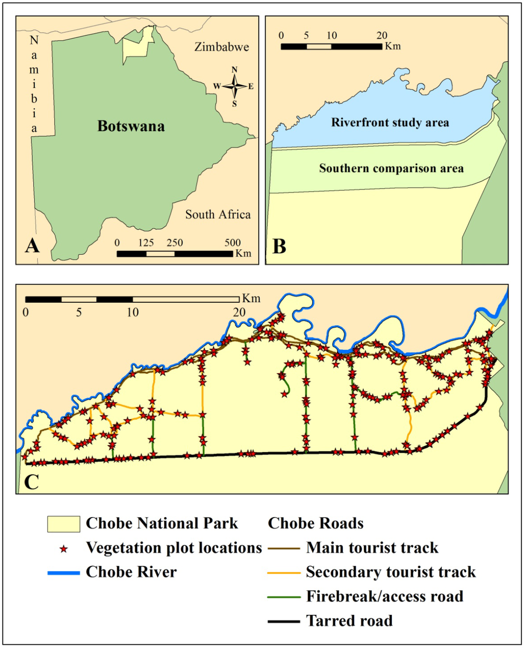
Figure 1.
Chobe National Park lies in the northeast corner of Botswana (A). The utility of the Moving Standard Deviation Index (MSDI) for identifying elephant impacts was assessed primarily along the Chobe riverfront, which was compared to an area of lower elephant utilization to the south (B). Elephant utilization of vegetation was assessed in 257 vegetation plots along the Chobe riverfront (C). Sampling was constrained to utilize roads and tracks due to the prevalence of wildlife in the park. Main tourist tracks are dirt tracks heavily utilized by tourists many times each day. Secondary tourist tracks experience moderate usage by tourists. Firebreaks and access roads are not open to the public and are rarely utilized. The tarred road is highly utilized by vehicles. All points were constrained to be at least 50 m from the tarred road to avoid negative influences of this traffic.

Chobe is home to a wide variety of wildlife, including 38 species of large mammals weighing more than 7 kg [71]. It also is inhabited by abundant bird species and provides a refuge for many birds of prey [72]. Chobe is most famously known, however, for its elephant population. Currently, northern Botswana has between 120,000–150,000 individuals, forming the largest population on the continent [29]. Chobe contains more elephants than any other protected area in Botswana with over 40,000 animals [29]. While elephant numbers are high within the park, densities in specific areas vary seasonally. Elephants concentrate along the Chobe riverfront in the dry season, resulting in local densities around 4 animals per km2, and then disperse southwards in the wet season as temporary pans fill with water, reducing riverfront densities to around 0.5 animals per km2 [73]. Concerns about the impacts of increasing numbers of elephants in Chobe on vegetation and wildlife have been voiced for the past 40 years [71] and have prompted a number of studies into the influences of elephants in this system [35,40,64,65,74]. Studies have shown dramatic changes in vegetation along the riverfront due to elephant impacts [64]. These effects are compounded by those of other large herbivores, which may prevent affected vegetation from regenerating [74,75].
Chobe National Park lies at the heart of the Kavango-Zambezi Transfrontier Conservation Area (KAZA TFCA). Formally established by treaty in 2011, this TFCA spans five countries (Angola, Botswana, Namibia, Zambia, and Zimbabwe) and will eventually cover between 250,000 to over 500,000 km2 [76,77]. One of the driving factors behind establishment of the TFCA is the desire to protect the largest continuous population of elephants in Africa, with around 250,000 individuals residing within and around the TFCA borders [76,77]. The KAZA TFCA will ultimately contain at least 36 national parks, game reserves, community conservancies, and game management areas with a goal of allowing movement of elephants and other species across international boundaries [76,77]. This conforms with recent calls for a metapopulation approach to managing elephant populations through the use of “megaparks” [78,79].
2.2. Remote Sensing Data Preparation and MSDI Calculation
Remote sensing data were obtained from the Moderate Resolution Imaging Spectroradiometer (MODIS). Initial assessment of multiple remote sensing products indicated that while Landsat 7 ETM+ offered higher spatial resolution, Scan Line Corrector issues for our study period made it unsuitable for our purposes. MODIS imagery at a 250 m resolution was the next best product available. The broader spatial scale of MODIS also fits well with management decisions made at landscape to regional scales, such as those spanning the Kavango-Zambezi Transfrontier Conservation Area. Level 3 images from the MOD09Q1 product were obtained from the USGS Land Processes Distributed Active Archive Center (LP DAAC) [80]. The Chobe riverfront study area, as well as a section of the park of approximately equal area to the south of the riverfront (see Section 2.3 below), were buffered by 500 m and extracted from MODIS tile H20V10. Further preprocessing, including projection and resampling, was conducted using the MODIS Reprojection Tool (MRT) [81]. The MOD09Q1 product is a two band (red: 620–670 nm; near infrared: 841–876 nm) 8-day composite. Each pixel contains the best observation across the 8-day period to eliminate imagery issues associated with clouds, aerosol loading, and shadow. Images were obtained for three dates: 14 April, 8 May, and 27 July 2012. The April image corresponds to the interannual stable period of greenness in the landscape, May is the start of the dry season when grass begins to die but woody vegetation retains greenness, July is the middle of the dry season and corresponds to our field sampling dates. While our field records of elephant utilization only match the final image, the browsing evidence we recorded is cumulative, meaning that our measures captured areas highly utilized by elephants in the April and May dates as well as in July. There is a possibility that some elephant utilization recorded in our field data occurred after the April and May image dates, but due to the relatively short time span this is not likely to have a major effect on our findings.
Subsequent analysis was performed on the red and near-infrared (NIR) MOD09Q1 bands, as well as three calculated spectral indices: the normalized difference vegetation index (NDVI), soil-adjusted vegetation index (SAVI), and modified soil-adjusted vegetation index (MSAVI2). Vegetation indices, also called spectral indices, assess savanna vegetation condition and monitor processes such as primary productivity [82,83,84,85,86]. Numerous studies have shown that satellite-derived vegetation indices are proxy measures of canopy greenness, cover, and structure [86]. The first index considered, NDVI, conveys plant “greenness” or photosynthetic activity [87]. It is one of the most commonly used vegetation indices and has played an influential role in wildlife ecology and management [88]. The index takes advantage of the fact that photosynthetically active vegetation absorbs red light and reflects NIR light [89,90]. With a theoretical range of −1 to +1, where +1 indicates high levels of photosynthetic activity, the index is calculated on a per-pixel basis according to the following formula [89,90]:
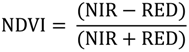
The SAVI index is used for landscapes with low vegetation cover and numerous exposed soil surfaces, similar to those seen along the Chobe riverfront. Regions with varying levels of exposed soil exhibit different amounts of reflected light in the red and NIR wavelengths. The SAVI index was developed as a modification of NDVI to correct for soil brightness when vegetation cover is low [51]. SAVI is calculated similarly to NDVI but includes a soil brightness correction factor (L) which is determined based on the amount of green vegetation in the study area [51]. Calculated on a per-pixel basis, SAVI uses the following formula [51]:
As with NDVI, the theoretical range of SAVI spans from −1 to +1 with +1 indicating higher levels of photosynthetic vegetation [51]. The last index included in this study, MSAVI2, is a revision of the modified soil-adjusted vegetation index (MSAVI). Like the SAVI index, MSAVI2 corrects for areas with a high degree of exposed soil. This index is a refinement of SAVI that minimizes user error in setting the correction factor by more reliably and simply calculating a soil brightness correction factor [91]. The index also ranges from −1 to +1 and is calculated per-pixel according to the following formula [91]:

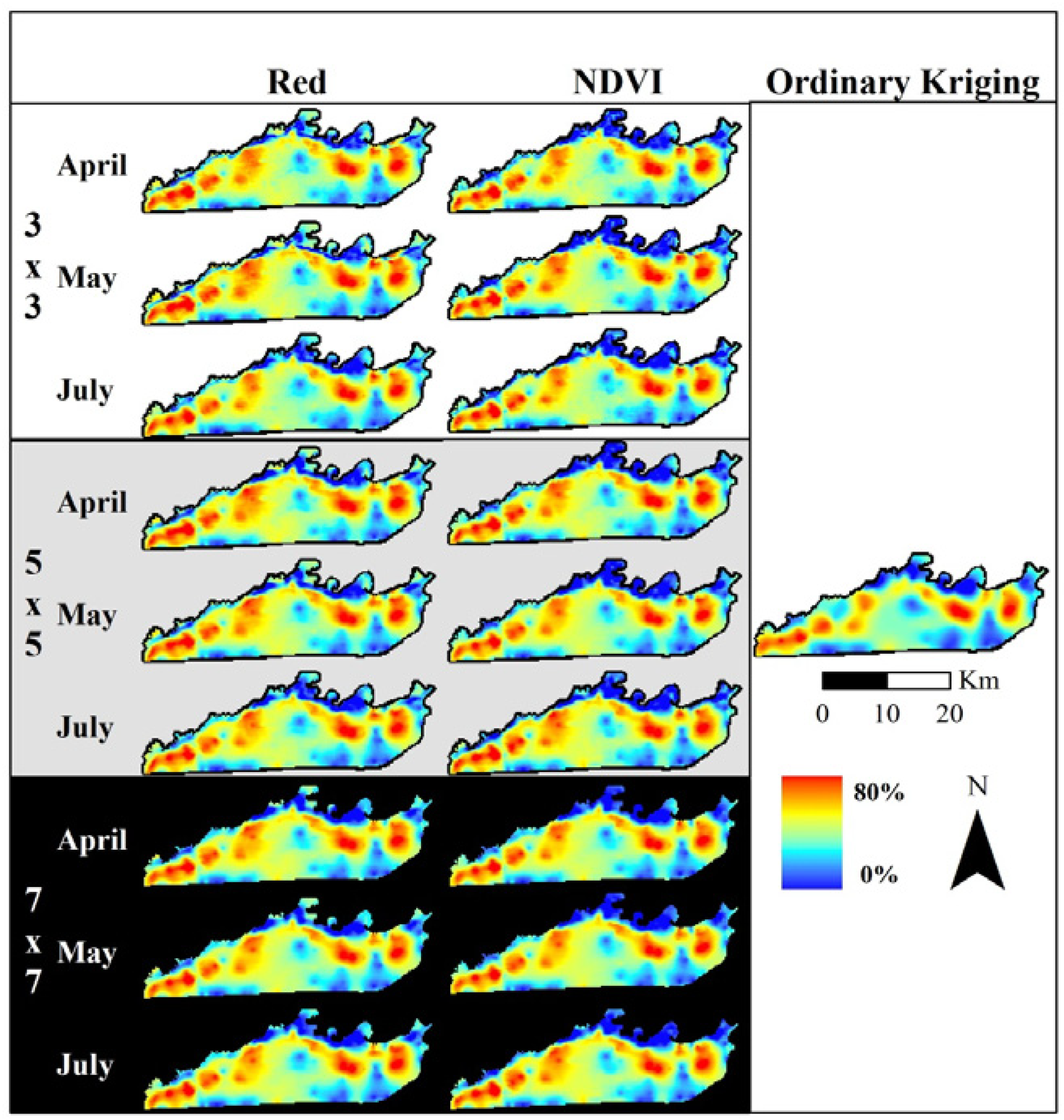
The MSDI for each band and date was calculated using a moving standard deviation window with the “raster” package [92] in the statistical program R [93]. Results were similar across bands so only the red band (Figure 2) and NDVI (Figure 3) are shown here for illustrative purposes. For NIR, SAVI, and MSAVI2, see Supplementary Materials Figures S1−S3. We varied the window size used in this analysis, assessing 3 × 3-, 5 × 5-, and 7 × 7-pixel moving windows. The calculation used to derive the MSDI results in an index that takes the units of the input data and has a minimum value of zero and a maximum value determined by the values of the pixels evaluated. Because of this variable maximum, MSDI values cannot be directly compared between bands, though general trends across bands can be assessed.
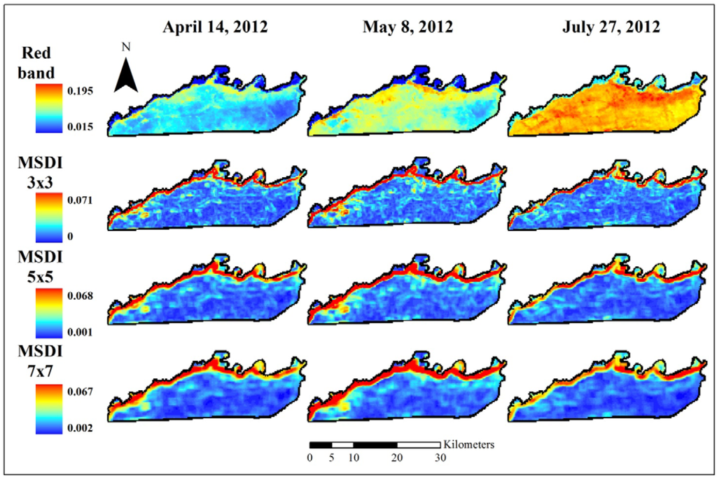
Figure 2.
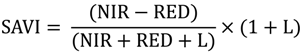
Red band MODIS data used to assess elephant utilization of vegetation along the Chobe riverfront, Chobe National Park, Botswana. The top row shows the base reflectance images for the three dates assessed in this project. Subsequent rows show the Moving Standard Deviation Index (MSDI) values calculated using 3 × 3-, 5 × 5-, and 7 × 7-pixel moving windows, respectively.
Figure 2.
Red band MODIS data used to assess elephant utilization of vegetation along the Chobe riverfront, Chobe National Park, Botswana. The top row shows the base reflectance images for the three dates assessed in this project. Subsequent rows show the Moving Standard Deviation Index (MSDI) values calculated using 3 × 3-, 5 × 5-, and 7 × 7-pixel moving windows, respectively.

2.3. Coarse Assessment of MSDI
The ability of the MSDI to discriminate between areas of higher and lower elephant utilization at a coarse scale was assessed by comparing the riverfront study area (high elephant utilization) with an area of approximately equal size to the south of the riverfront (low elephant utilization; Figure 1B). Dung counts conducted in the riverfront and southern areas during a previous study investigating elephant impacts on trees in Chobe National Park [65,94] were used to compare relative elephant density in areas north and south of the main tarred road. Previous research has indicated a positive relationship between elephant density and utilization levels in similar systems [95]. Dung counts were collected during a similar time of year as the imagery used in this study [94] and should reflect utilization patterns during the study period. Dung plots counted all elephant dung within a 10 × 100 m transect to give an estimate of relative animal use of sites [94,96]. While issues have been raised about the use of dung counts to measure mammal densities [97], Barnes [98] showed that they are as effective as other methods of estimation for elephants. MSDI values were extracted from 200 random points in each section. Equality of variances for the two samples was assessed using Fisher’s F-test [99]. Based on F-test results, mean MSDI values for the two areas were compared using an unequal variance t-test [100]. This procedure was repeated 100 times for each MSDI band and date to assess stability of observed patterns.

Figure 3.
Normalized difference vegetation index (NDVI) data used to assess elephant utilization of vegetation along the Chobe riverfront, Chobe National Park, Botswana. The top row shows the base images for the three dates assessed in this project. Subsequent rows show the Moving Standard Deviation Index (MSDI) values calculated using 3 × 3-, 5 × 5-, and 7 × 7-pixel moving windows, respectively. These indices are unitless. NDVI ranges from −1 to +1 while the MSDI has a minimum value of zero and a maximum determined by the data.

2.4. Fine Assessment of MSDI
MSDI maps for the riverfront area of Chobe National Park were assessed against quantitative vegetation plots to investigate the ability of the MSDI to identify elephant utilization at finer scales.
2.4.1. Field Data Collection
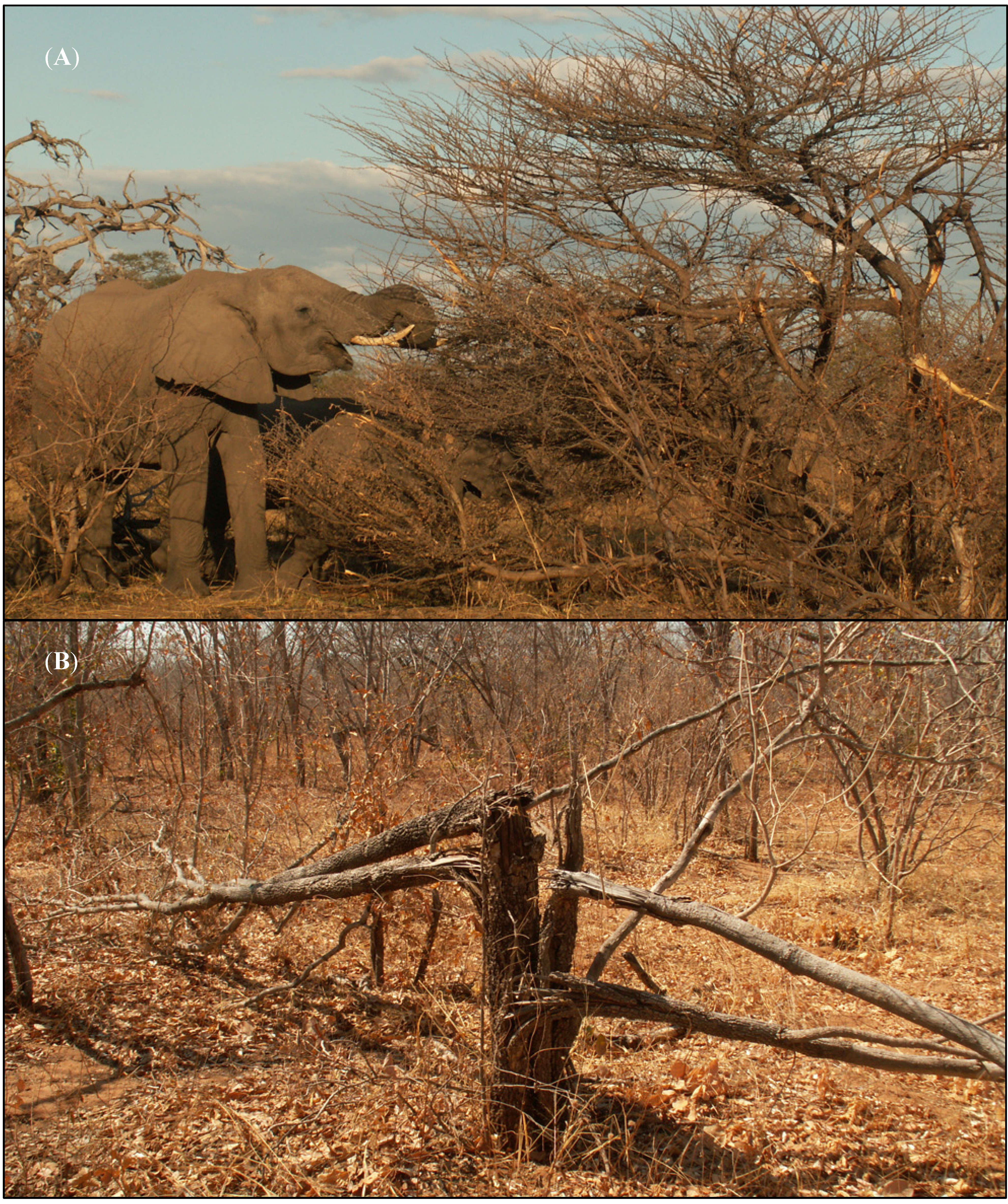
Field data assessing utilization of vegetation by elephants were collected from mid-July to early August 2012. A total of 257 vegetation plots were assessed in the Chobe riverfront area (Figure 1C). Vegetation plots covered a 60 × 60 m area with records made of the percentage of woody vegetation highly utilized by elephants. Elephant browsing is distinctive, easily differentiating plants utilized by elephants from those browsed by other species (pers. obs.). Trees were considered highly utilized if elephants had removed major branches or if the main meristem was broken (Figure 4). In addition, percent coverage of woody vegetation was visually estimated by two observers, with any discrepancies averaged to produce final values.
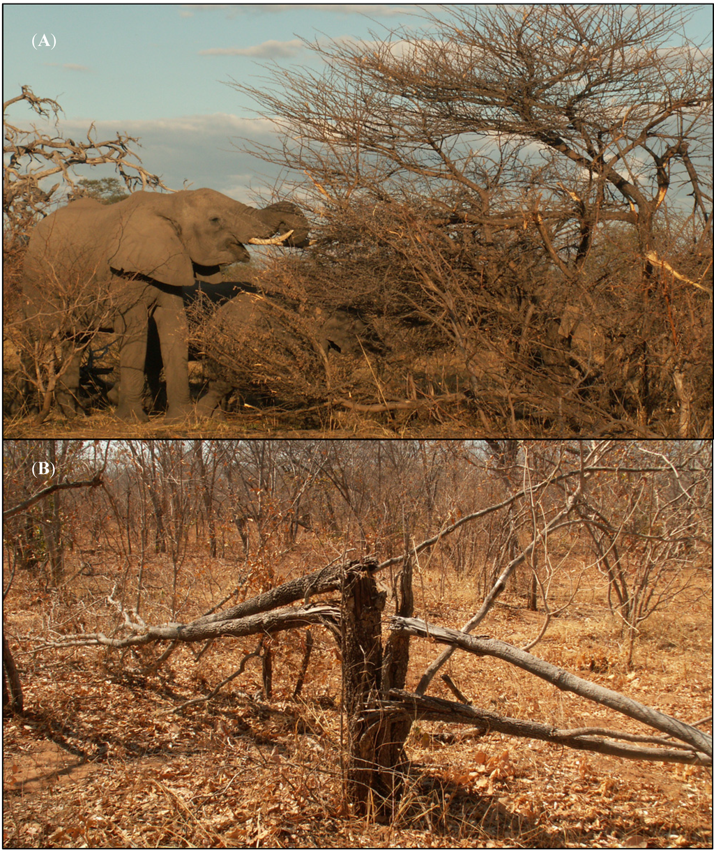
Figure 4.
(A) Elephant browsing on woody vegetation. Note the obvious evidence of past utilization on the tree to the right. (B) High elephant utilization in Chobe National Park. Elephants often break large branches and knock over trees while foraging. Photo credit: T. Fullman.
Figure 4.
(A) Elephant browsing on woody vegetation. Note the obvious evidence of past utilization on the tree to the right. (B) High elephant utilization in Chobe National Park. Elephants often break large branches and knock over trees while foraging. Photo credit: T. Fullman.
Vegetation plot locations were randomly generated using the randomPoints function of the “dismo” package in R [101]. Plots were constrained to be at least 100 m apart. In addition, the prevalence of wildlife in the park necessitated that plots be assessed within 100 m of roads. The “roads” in Chobe, however, varied greatly from a main tarred road to dirt tracks regularly used by tourists, to firebreaks and access roads infrequently traveled (Figure 1C). Plots were constrained to be at least 50 m away from the tarred road to minimize road-based effects [64,102]. Dirt tracks and firebreaks were allowed to be closer to plots, as elephants regularly utilize these areas. Seventy vegetation plots (27.24%) included tracks and firebreaks. Mann-Whitney U-tests for variance of means and Analysis of Covariance (ANCOVA) tests of subset regression equations showed no difference between samples with and without tracks, so all samples were combined in subsequent analyses.
2.4.2. Statistical Analysis
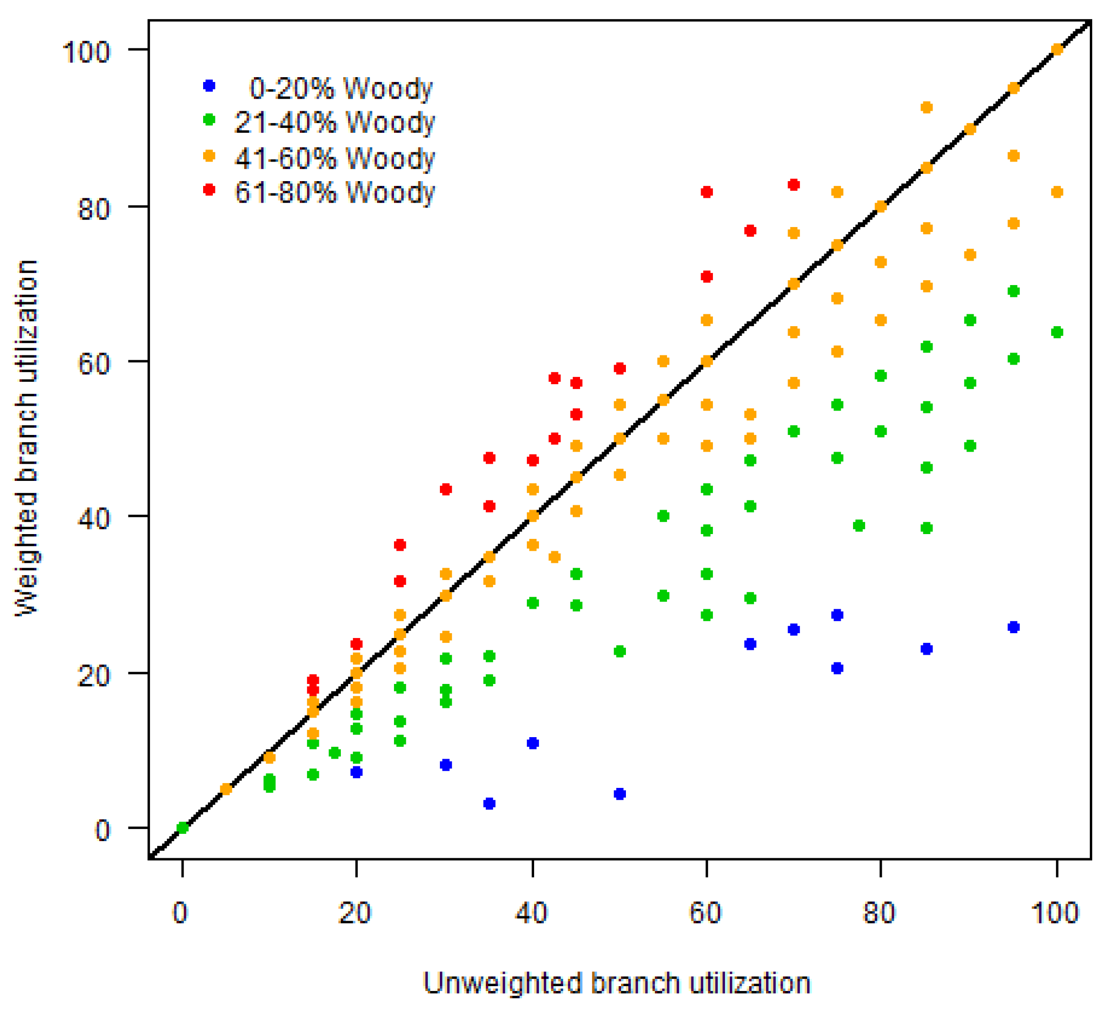
To better account for interactions between woody cover and elephant utilization, a weighted measure of utilization was calculated. The level of elephant utilization for a plot was assessed independently of the percentage of woody vegetation in the plot (i.e., A plot containing 25% trees, all of which were highly utilized, and a plot with 50% trees, all highly utilized, would each have received an elephant utilization score of 100%). To make these more directly comparable, we calculated a weighted measure of elephant utilization according to the following formula:
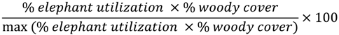
This weighted measure penalizes the utilization values of plots with few trees and emphasizes those with higher woody cover (Figure 5), following the idea that plots with high utilization but low woody cover are likely to have different MSDI signatures than those with high utilization and high woody cover.
Local and global Moran’s I tests [103,104] were used to check for spatial autocorrelation in the vegetation plot data. Failing to incorporate spatial autocorrelation in regression models can lead to incorrect statistical inference from inefficient or biased parameter estimates [105]. To avoid this, spatial simultaneous autoregressive (SAR) models were fit between weighted elephant utilization and MSDI values in Chobe [106]. For an overview of SAR models as well as their implementation in R, see Kissling and Carl [107]. Spatial SAR models can be fit in a spatial lag or spatial error form. Spatial error models include autocorrelation in the error term, as
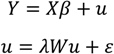 where, as in Ordinary Least Squares (OLS) regression, β is the vector of slopes associated with the explanatory variables X. Unlike in OLS regression, however, the error term, u, is spatially weighted using the weights matrix, W, and the spatial error coefficient, λ. Remaining uncorrelated error is indicated by ε. Spatial error models tend to be used in situations where spatial autocorrelation is not fully explained by the explanatory variables [107]. Spatial lag models, on the other hand, assume that spatial structure comes from factors that are an inherent property of the response variable itself and so include a spatially lagged dependent variable as an additional predictor. Such models follow the form
where ρ is the spatial coefficient and the other terms are the same as in Equation (5). Spatial weights matrices used to develop models were determined using neighborhood distances of 4000 m based on analysis of autocorrelation using variograms. Row standardization was used in developing weights matrices since points had unequal numbers of neighbors [108]. Lagrange Multiplier tests [109] were used to determine which type of spatial model (i.e., spatial error or spatial lag) was best suited to each predictor variable. Moran’s I tests, Lagrange Multiplier tests and SAR models were run using the “spdep” package in R [110].
where, as in Ordinary Least Squares (OLS) regression, β is the vector of slopes associated with the explanatory variables X. Unlike in OLS regression, however, the error term, u, is spatially weighted using the weights matrix, W, and the spatial error coefficient, λ. Remaining uncorrelated error is indicated by ε. Spatial error models tend to be used in situations where spatial autocorrelation is not fully explained by the explanatory variables [107]. Spatial lag models, on the other hand, assume that spatial structure comes from factors that are an inherent property of the response variable itself and so include a spatially lagged dependent variable as an additional predictor. Such models follow the form
where ρ is the spatial coefficient and the other terms are the same as in Equation (5). Spatial weights matrices used to develop models were determined using neighborhood distances of 4000 m based on analysis of autocorrelation using variograms. Row standardization was used in developing weights matrices since points had unequal numbers of neighbors [108]. Lagrange Multiplier tests [109] were used to determine which type of spatial model (i.e., spatial error or spatial lag) was best suited to each predictor variable. Moran’s I tests, Lagrange Multiplier tests and SAR models were run using the “spdep” package in R [110].
Y = ρWY + Xβ + ε
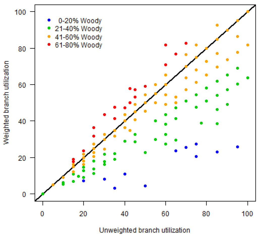
Figure 5.
Relationship between unweighted and weighted measures of elephant utilization along the Chobe riverfront, Botswana. The 1:1 line is indicated in black for comparison. The weighted utilization measure penalizes the values of plots with few trees (blue and green), shifting them below the 1:1 line, and emphasizes those with higher woody cover (red), shifting them above the line. See text for details.
Kriging was used to enable assessment of elephant utilization at scales finer than the 250 m resolution of a MODIS pixel. Originally developed to assist in mining operations, kriging enables interpolated mapping of a physical process, based on analysis of spatially explicit data [111,112]. Here the process of interest is elephant utilization of vegetation, with the vegetation plots serving as observations of a continuous underlying process of utilization. Ordinary kriging uses only information about the spatial relationship between observations and does not include any explanatory covariates [106,113], allowing assessment that is independent of the 250 m MODIS pixel size. In addition, universal kriging was conducted using MSDI as the explanatory covariate. This approach allows the mean of the modeled process to vary according to explanatory covariates in a regression-like framework [106,113]. Comparing ordinary and universal kriging approaches allowed assessment of whether observed trends changed with inclusion of MODIS-scale MSDI values. Kriging was carried out in the “gstat” package in R [114]. Kriging models were assessed via leave-one-out cross validation [115,116].
2.4.3. Assessment of Alternative Covariates
To assess the degree to which other environmental covariates might be driving observed MSDI patterns we assessed the correlation of each MSDI date and band with nine covariates. The covariates assessed were elevation, slope, distance to the Chobe River, distance to roads/tracks, vegetation class, latitude and longitude, and two hydrology measures—flow direction, reflecting the path water is expected to take across a landscape, and flow accumulation, reflecting where water on a landscape is expected to aggregate. Elevation was obtained from the ASTER Global Digital Elevation Model (ASTER GDEM is a product of METI and NASA), which presents elevation at a 30 × 30 m spatial resolution. Slope and hydrology layers were derived from the elevation layer in ArcGIS (version 9.3, ESRI Inc., Redlands, CA, USA). Distance to roads was determined from shapefiles combined with self-generated GPS tracks. Vegetation classes were derived from White’s vegetation map [117]. A systematic grid of approximately 500 points, spaced at least 250 m apart, was used to sample covariates in each of the riverfront and southern sections of the park (Figure 1B). The correlation was assessed between these covariates and MSDI values sampled at the same locations.
To assess the effect that the Chobe River and main tourist tracks might have on our regression findings we subset the field data from the riverfront and ran additional spatial regression analyses on the subset data. Points lying within 250 m of the main tourist tracks lining the Chobe River (Figure 1C) were extracted as the river subset. They were compared against the inland subset—all points greater than 250 m from main tourist tracks. Spatial regression analyses as described above were conducted on each subset to evaluate the relationship between the MSDI and elephant utilization.
3. Results
3.1. Coarse Assessment of MSDI
Dung density levels were significantly higher for elephants in the riverfront study area compared to the southern section (Mann-Whitney U test p < 0.05). Fisher’s F-test results for each of the 100 iterations of every band and date combination showed strongly significant results (p < 0.0001), indicating unequal variance in MSDI values between riverfront and southern sections. In light of this, unequal variance t-tests were run for each band, date, and iteration. Results were strongly significant for each of these tests (t range = 2.97–13.18, df range = 201–272, all p < 0.005), with MSDI values higher in the riverfront section compared to the southern section. Thus, MSDI values were significantly higher in areas of higher elephant dung density, revealing increased heterogeneity at a landscape scale in areas used heavily by elephants.
3.2. Fine Assessment of MSDI
3.2.1. Regression Assessment of Elephant Utilization
Local and global Moran’s I tests indicated significant spatial structure in the weighted elephant utilization data, necessitating use of spatial regression models. Lagrange Multiplier tests showed spatial structure in the Chobe National Park elephant utilization dataset was best accounted for using spatial error models for all bands, indices, and window sizes except the 3 × 3 SAVI and MSAVI2 models for 27 July, which had a slightly more significant spatial lag rather than spatial error model. However, Kissling and Carl [107] found that spatial lag models showed less consistent results than spatial error models, leading to higher likelihood of bias. In light of this, and to maintain consistency, we used a spatial error model for these data as well. Doing so did not greatly alter any of the regression parameters.
The relationship between elephant utilization and MSDI values was consistent across all bands, image dates, and window sizes (Table 1). Weighted elephant utilization was negatively related to MSDI values in all models and showed highly significant relationships (all p < 0.005). Model comparison via Akaike Information Criterion (AIC) [118,119] indicated better model fit for all spatial models compared to non-spatial Ordinary Least Squares (OLS) models (Table 1). While all regression coefficients were highly significant, the explanatory power of these relationships, as described by the coefficient of determination (R2) was generally low, with values ranging between 0.11 and 0.24 (Table 1).

Table 1.
Spatial regression results for weighted elephant utilization in the riverfront region of Chobe National Park, Botswana. See Equation (5) in the text for spatial error simultaneous autoregressive model formulation. Values in parentheses indicate standard error estimates for regression parameters. All estimates have p < 0.005 (n = 257 for all models). All dates are in 2012.
| Image | Window | Date | Intercept | MSDI | Lambda | RMSE | R2 | ΔAIC | |||
|---|---|---|---|---|---|---|---|---|---|---|---|
| Red | 3 × 3 | 14/4 | 50.120 | (3.857) | −824.476 | (124.373) | 0.631 | (0.101) | 20.69 | 0.22 | 23.1 |
| 8/5 | 49.039 | (3.934) | −601.929 | (88.871) | 0.648 | (0.098) | 20.61 | 0.23 | 24.9 | ||
| 27/7 | 46.934 | (3.549) | −674.380 | (148.144) | 0.575 | (0.112) | 21.59 | 0.16 | 16.7 | ||
| 5 × 5 | 14/4 | 52.748 | (4.388) | −850.280 | (122.238) | 0.673 | (0.093) | 20.51 | 0.24 | 27.6 | |
| 8/5 | 50.096 | (4.170) | −531.774 | (87.233) | 0.653 | (0.097) | 20.91 | 0.21 | 24.9 | ||
| 27/7 | 49.925 | (3.889) | −742.468 | (130.328) | 0.615 | (0.104) | 21.11 | 0.19 | 20.4 | ||
| 7 × 7 | 14/4 | 53.283 | (4.546) | −811.058 | (130.336) | 0.669 | (0.093) | 20.85 | 0.21 | 25.7 | |
| 8/5 | 50.040 | (4.202) | −473.364 | (90.751) | 0.637 | (0.100) | 21.29 | 0.18 | 22.3 | ||
| 27/7 | 50.046 | (4.034) | −674.057 | (128.717) | 0.619 | (0.103) | 21.30 | 0.18 | 20.3 | ||
| NIR | 3 × 3 | 14/4 | 47.391 | (3.531) | −326.513 | (46.806) | 0.616 | (0.104) | 20.55 | 0.24 | 20.6 |
| 8/5 | 47.356 | (3.724) | −282.070 | (40.693) | 0.638 | (0.100) | 20.55 | 0.24 | 23.0 | ||
| 27/7 | 45.927 | (3.338) | −365.119 | (92.122) | 0.541 | (0.118) | 21.83 | 0.14 | 13.5 | ||
| 5 × 5 | 14/4 | 48.374 | (3.919) | −298.169 | (43.662) | 0.651 | (0.097) | 20.59 | 0.23 | 23.6 | |
| 8/5 | 47.707 | (3.903) | −233.403 | (38.227) | 0.642 | (0.099) | 20.92 | 0.21 | 22.8 | ||
| 27/7 | 48.385 | (3.586) | −418.671 | (82.998) | 0.575 | (0.112) | 21.41 | 0.17 | 16.2 | ||
| 7 × 7 | 14/4 | 48.565 | (4.010) | −269.858 | (43.968) | 0.648 | (0.098) | 20.90 | 0.21 | 22.7 | |
| 8/5 | 47.750 | (3.934) | −205.667 | (38.498) | 0.632 | (0.101) | 21.24 | 0.18 | 21.2 | ||
| 27/7 | 48.468 | (3.747) | −386.700 | (83.097) | 0.584 | (0.110) | 21.55 | 0.16 | 16.8 | ||
| NDVI | 3 × 3 | 14/4 | 48.601 | (3.580) | −213.858 | (44.825) | 0.561 | (0.114) | 21.53 | 0.16 | 16.0 |
| 8/5 | 47.277 | (3.482) | −192.491 | (34.795) | 0.586 | (0.110) | 21.21 | 0.19 | 18.0 | ||
| 27/7 | 46.938 | (3.479) | −429.337 | (94.926) | 0.564 | (0.114) | 21.61 | 0.15 | 16.4 | ||
| 5 × 5 | 14/4 | 50.779 | (4.328) | −206.896 | (40.974) | 0.638 | (0.100) | 21.35 | 0.17 | 22.9 | |
| 8/5 | 49.110 | (3.752) | −175.571 | (33.094) | 0.597 | (0.108) | 21.29 | 0.18 | 18.7 | ||
| 27/7 | 49.559 | (3.816) | −427.776 | (76.246) | 0.608 | (0.106) | 21.16 | 0.19 | 21.0 | ||
| 7 × 7 | 14/4 | 50.412 | (4.504) | −175.691 | (40.219) | 0.637 | (0.100) | 21.60 | 0.15 | 21.9 | |
| 8/5 | 49.905 | (4.026) | −164.583 | (31.986) | 0.617 | (0.104) | 21.33 | 0.18 | 19.8 | ||
| 27/7 | 50.220 | (3.941) | −404.006 | (73.008) | 0.614 | (0.104) | 21.18 | 0.19 | 21.3 | ||
| SAVI | 3 × 3 | 14/4 | 48.743 | (3.436) | −318.769 | (52.687) | 0.576 | (0.112) | 21.00 | 0.20 | 17.1 |
| 8/5 | 47.949 | (3.537) | −321.785 | (51.739) | 0.601 | (0.107) | 20.90 | 0.21 | 19.2 | ||
| 27/7 | 44.719 | (3.341) | −415.079 | (145.690) | 0.522 | (0.122) | 22.16 | 0.11 | 12.2 | ||
| 5 × 5 | 14/4 | 49.486 | (3.887) | −275.062 | (48.632) | 0.619 | (0.103) | 21.13 | 0.19 | 20.7 | |
| 8/5 | 48.114 | (3.789) | −255.448 | (48.091) | 0.612 | (0.105) | 21.27 | 0.18 | 19.8 | ||
| 27/7 | 47.986 | (3.618) | −554.728 | (126.871) | 0.562 | (0.114) | 21.67 | 0.15 | 16.1 | ||
| 7 × 7 | 14/4 | 49.351 | (4.045) | −238.349 | (47.728) | 0.621 | (0.103) | 21.39 | 0.17 | 20.4 | |
| 8/5 | 47.926 | (3.884) | −217.275 | (46.835) | 0.608 | (0.105) | 21.53 | 0.16 | 19.1 | ||
| 27/7 | 48.700 | (3.799) | −550.661 | (127.308) | 0.574 | (0.112) | 21.67 | 0.15 | 17.1 | ||
| MSAVI2 | 3 × 3 | 14/4 | 48.834 | (3.410) | −338.572 | (56.729) | 0.569 | (0.113) | 21.04 | 0.20 | 16.4 |
| 8/5 | 48.073 | (3.526) | −350.666 | (56.679) | 0.598 | (0.107) | 20.92 | 0.21 | 18.9 | ||
| 27/7 | 44.804 | (3.333) | −428.316 | (149.076) | 0.519 | (0.122) | 22.15 | 0.11 | 11.9 | ||
| 5 × 5 | 14/4 | 49.652 | (3.851) | −295.497 | (52.541) | 0.612 | (0.105) | 21.15 | 0.19 | 20.0 | |
| 8/5 | 48.106 | (3.776) | −275.033 | (52.561) | 0.609 | (0.105) | 21.31 | 0.18 | 19.5 | ||
| 27/7 | 48.144 | (3.609) | −581.133 | (132.513) | 0.558 | (0.115) | 21.67 | 0.15 | 15.7 | ||
| 7 × 7 | 14/4 | 49.419 | (4.006) | −253.828 | (51.741) | 0.613 | (0.105) | 21.43 | 0.17 | 19.6 | |
| 8/5 | 47.857 | (3.854) | −233.194 | (51.171) | 0.603 | (0.106) | 21.56 | 0.16 | 18.6 | ||
| 27/7 | 48.764 | (3.776) | −573.581 | (132.332) | 0.570 | (0.113) | 21.67 | 0.15 | 16.6 | ||
Note: NIR = Near Infrared; NDVI = Normalized Difference Vegetation Index; SAVI = Soil-Adjusted Vegetation Index; MSAVI2 = Modified Soil-Adjusted Vegetation Index; RMSE = Root mean square error; ΔAIC indicates the difference in the Akaike Information Criterion between the spatial and non-spatial forms of the regression model (AICnon-spatial—AICspatial), thus positive ΔAIC indicates model improvement over the non-spatial form.
While model fits were similar across dates and bands, the 7 × 7-pixel window size consistently showed the worst performance in terms of root mean square error (RMSE) and R2 values when looking across the three image dates. Beyond this, the various bands and indices differed in whether better performance was obtained with a 3 × 3- or 5 × 5-pixel window size. The MSDI values calculated using NIR, SAVI, and MSAVI2 showed highest performance for a 3 × 3-pixel window size while the red band and NDVI showed highest performance at a 5 × 5-pixel window size. Averaging across the three window sizes, model results generally showed highest performance in April and May, with the exception of NDVI, which occasionally displayed comparable July values. Model results for the 3 × 3-pixel window sizes were consistently best in May while model results for the 5 × 5 and 7 × 7 window sizes were generally best in April, with the exception of NDVI where they exhibited their highest R2 and lowest RMSE values in July.
3.2.2. Kriging Assessment of Elephant Utilization
Fitted variogram models for both ordinary and universal kriging are given in Table 2. All models indicated the highest levels of elephant utilization of woody vegetation were patchily distributed and found at intermediate distances from the river’s edge. Ordinary kriging of elephant utilization was best modeled using a spherical variogram while universal kriging models all utilized exponential variograms. Ordinary kriging suggested a higher range than universal kriging models but otherwise had similar results (Table 2). As with the regression results, model parameters (range, sill, and nugget) from models considering MSDI were similar across dates, bands and indices (Table 2). Cross-validation showed similar results between ordinary kriging and universal kriging in terms of RMSE and R2 values. While moderate overall, explanatory power for the kriging models was higher than that for the regression models (R2 range = 0.34–0.41 for kriging and 0.11–0.24 for regression). Values for RMSE were slightly lower for kriging compared to regression models (RMSE range = 18.05–19.06 for kriging and 20.51–22.16 for regression). Predictions of weighted elephant utilization were highly similar across all dates, images, and window sizes under universal kriging (Figure 6, Supplementary Materials Figure S4).
Table 2.
Kriging variogram parameters and cross-validation results for weighted elephant utilization in the Chobe riverfront, Chobe National Park, Botswana. n = 257 for all models.
| Method | Covariate | Window | Date | Variogram | Range | Sill | Nugget | RMSE | R2 |
|---|---|---|---|---|---|---|---|---|---|
| Ordinary | Constant | Spherical | 3,653 | 592 | 251 | 18.85 | 0.36 | ||
| Universal | Red | 3 × 3 | 4/14/2012 | Exponential | 1,314 | 512 | 185 | 18.50 | 0.38 |
| 5/8/2012 | Exponential | 1,342 | 517 | 158 | 18.21 | 0.40 | |||
| 7/27/2012 | Exponential | 1,291 | 552 | 181 | 18.88 | 0.35 | |||
| 5 × 5 | 4/14/2012 | Exponential | 1,400 | 515 | 185 | 18.27 | 0.40 | ||
| 5/8/2012 | Exponential | 1,392 | 531 | 185 | 18.37 | 0.39 | |||
| 7/27/2012 | Exponential | 1,429 | 537 | 189 | 18.45 | 0.38 | |||
| 7 × 7 | 4/14/2012 | Exponential | 1,365 | 527 | 189 | 18.50 | 0.38 | ||
| 5/8/2012 | Exponential | 1,322 | 541 | 187 | 18.65 | 0.37 | |||
| 7/27/2012 | Exponential | 1,369 | 545 | 185 | 18.54 | 0.38 | |||
| NIR | 3 × 3 | 4/14/2012 | Exponential | 1,350 | 506 | 183 | 18.32 | 0.39 | |
| 5/8/2012 | Exponential | 1,390 | 516 | 160 | 18.05 | 0.41 | |||
| 7/27/2012 | Exponential | 1,219 | 557 | 183 | 18.96 | 0.35 | |||
| 5 × 5 | 4/14/2012 | Exponential | 1,497 | 517 | 203 | 18.34 | 0.39 | ||
| 5/8/2012 | Exponential | 1,495 | 533 | 201 | 18.41 | 0.39 | |||
| 7/27/2012 | Exponential | 1,341 | 540 | 194 | 18.59 | 0.37 | |||
| 7 × 7 | 4/14/2012 | Exponential | 1,443 | 527 | 206 | 18.54 | 0.38 | ||
| 5/8/2012 | Exponential | 1,399 | 541 | 202 | 18.66 | 0.37 | |||
| 7/27/2012 | Exponential | 1,264 | 546 | 178 | 18.68 | 0.37 | |||
| NDVI | 3 × 3 | 4/14/2012 | Exponential | 1,243 | 541 | 164 | 18.73 | 0.36 | |
| 5/8/2012 | Exponential | 1,227 | 532 | 134 | 18.26 | 0.40 | |||
| 7/27/2012 | Exponential | 1,194 | 548 | 149 | 18.77 | 0.36 | |||
| 5 × 5 | 4/14/2012 | Exponential | 1,305 | 550 | 167 | 18.64 | 0.37 | ||
| 5/8/2012 | Exponential | 1,321 | 538 | 181 | 18.64 | 0.37 | |||
| 7/27/2012 | Exponential | 1,286 | 532 | 159 | 18.40 | 0.39 | |||
| 7 × 7 | 4/14/2012 | Exponential | 1,276 | 560 | 171 | 18.82 | 0.36 | ||
| 5/8/2012 | Exponential | 1,327 | 542 | 185 | 18.75 | 0.36 | |||
| 7/27/2012 | Exponential | 1,313 | 534 | 174 | 18.44 | 0.38 | |||
| SAVI | 3 × 3 | 4/14/2012 | Exponential | 1,234 | 517 | 170 | 18.52 | 0.38 | |
| 5/8/2012 | Exponential | 1,286 | 522 | 152 | 18.20 | 0.40 | |||
| 7/27/2012 | Exponential | 1,128 | 567 | 166 | 19.05 | 0.34 | |||
| 5 × 5 | 4/14/2012 | Exponential | 1,357 | 533 | 191 | 18.59 | 0.37 | ||
| 5/8/2012 | Exponential | 1,347 | 539 | 190 | 18.62 | 0.37 | |||
| 7/27/2012 | Exponential | 1,199 | 546 | 169 | 18.81 | 0.36 | |||
| 7 × 7 | 4/14/2012 | Exponential | 1,319 | 543 | 190 | 18.74 | 0.36 | ||
| 5/8/2012 | Exponential | 1,304 | 547 | 193 | 18.81 | 0.36 | |||
| 7/27/2012 | Exponential | 1,181 | 547 | 162 | 18.81 | 0.36 | |||
| Universal | MSAVI2 | 3 × 3 | 4/14/2012 | Exponential | 1,215 | 518 | 170 | 18.55 | 0.38 |
| 5/8/2012 | Exponential | 1,276 | 522 | 152 | 18.22 | 0.40 | |||
| 7/27/2012 | Exponential | 1,123 | 566 | 169 | 19.06 | 0.34 | |||
| 5 × 5 | 4/14/2012 | Exponential | 1,347 | 532 | 191 | 18.60 | 0.37 | ||
| 5/8/2012 | Exponential | 1,344 | 540 | 190 | 18.63 | 0.37 | |||
| 7/27/2012 | Exponential | 1,201 | 545 | 174 | 18.81 | 0.36 | |||
| 7 × 7 | 4/14/2012 | Exponential | 1,309 | 543 | 190 | 18.75 | 0.36 | ||
| 5/8/2012 | Exponential | 1,296 | 548 | 193 | 18.81 | 0.36 | |||
| 7/27/2012 | Exponential | 1,160 | 545 | 161 | 18.82 | 0.36 |
Note: NIR = Near Infrared; NDVI = Normalized Difference Vegetation Index; SAVI = Soil-Adjusted Vegetation Index; MSAVI2 = Modified Soil-Adjusted Vegetation Index; RMSE = Root mean square error; Units for range, sill and nugget are meters.

Figure 6.
Percent elephant utilization interpolated across the Chobe riverfront using universal kriging with the Moving Standard Deviation Index (MSDI) as the explanatory variable and ordinary kriging considering only vegetation plot data. The white, grey, and black sections indicate the three window sizes used for MSDI calculations while rows within sections indicate the imagery dates. The ordinary kriging prediction is only based on field data and does not conform to any particular date. Results for the near-infrared band and the SAVI and MSAVI2 indices were highly similar and are presented in the Supplementary Materials, Figure S4.
As with the regression models, model performance in terms of RMSE and R2 was worst for universal kriging using the 7 × 7-pixel window MSDI images. Additionally, results for July images displayed lower R2 and higher RMSE values than those for April or May, with the exception of NDVI. Once again, SAVI and MSAVI2 showed higher performance using a 3 × 3-pixel window size, when averaging across dates, while the red band and NDVI showed better performance with a 5 × 5-pixel window size. The validation data for MSDI calculated on the NIR band showed equal performance for 3 × 3- and 5 × 5-pixel window sizes. May images generally provided the best performance, once again with the exception of NDVI.
3.3. Assessment of Alternative Covariates
Pearson’s correlation coefficients between alternative environmental covariates and MSDI values are given for the Chobe riverfront and southern comparison area (Figure 1B) in Table 3 and Table 4, respectively. The relationship between covariates and MSDI values was generally weak across all dates and bands. One exception to this occurred in the riverfront study area. In this area, distance to the Chobe River and elevation (themselves strongly correlated, r = 0.868), had moderately negative relationships (range: −0.773 to −0.425) with all MSDI bands (Table 3). There were no strong correlations in the southern comparison area (Table 4).
To further investigate the effect of the Chobe River, field data were subset into river and inland groups (see Methods for details) and spatial regression models were evaluated. The relationship between elephant utilization and MSDI was generally maintained for the river subset (Supplementary Materials Table S1), but broke down for the inland subset (Supplementary Materials Table S2). For the river subset, the negative relationship between MSDI and elephant utilization remained significant for all dates and window sizes for NDVI, and most dates and window sizes for the red and NIR bands (Supplementary Materials Table S1). The SAVI and MSAVI2 indices were less consistent, exhibiting a number of non-significant relationships (Supplementary Materials Table S1). In the inland subset, only the red band displayed significant relationships between MSDI and elephant utilization, all other bands and indices were insignificant (Supplementary Materials Table S2). Interestingly, the relationship between MSDI and elephant utilization changed to be positive in the inland subset for the red band.
4. Discussion
The ability of the Moving Standard Deviation Index (MSDI) to identify elephant-modification of vegetation was assessed in Chobe National Park, Botswana. At a coarse scale, MSDI values were significantly higher in a region with higher elephant utilization, compared to a less utilized region. At a finer scale, focusing on just the highly utilized Chobe riverfront, weighted elephant utilization showed a negative relationship with MSDI values (Table 1), reversing the coarse-scale trend. Assessment of alternative covariates that could influence the observed patterns suggested that proximity to the Chobe River might be correlated with higher MSDI values (Table 3). Subset models built on river and inland vegetation plots affirmed that while the negative relationship between MSDI and elephant utilization was generally maintained for the river subset (Supplementary Materials Table S1), it was mostly non-significant for the inland subset (Supplementary Materials Table S2).
Table 3.
Pearson’s correlation coefficients between environmental covariates and Moving Standard Deviation Index (MSDI) values along the Chobe riverfront, Botswana. All dates are in 2012.
| Image | Window | Date | Long. | Lat. | Elev. | Dist. Road | Dist. River | Flow Acc. | Flow Dir. | Slope | Veg. Class |
|---|---|---|---|---|---|---|---|---|---|---|---|
| Red | 3 × 3 | 14/4 | −0.150 | 0.357 | −0.590 | −0.254 | −0.492 | 0.061 | 0.024 | 0.218 | 0.337 |
| 8/5 | −0.149 | 0.304 | −0.543 | −0.286 | −0.471 | 0.047 | 0.032 | 0.226 | 0.314 | ||
| 27/7 | 0.003 | 0.419 | −0.594 | −0.238 | −0.456 | 0.026 | −0.025 | 0.165 | 0.310 | ||
| 5 × 5 | 14/4 | −0.135 | 0.469 | −0.709 | −0.302 | −0.600 | 0.037 | 0.032 | 0.162 | 0.401 | |
| 8/5 | −0.122 | 0.427 | −0.679 | −0.346 | −0.590 | 0.018 | 0.036 | 0.176 | 0.382 | ||
| 27/7 | −0.013 | 0.513 | −0.700 | −0.299 | −0.568 | 0.000 | −0.001 | 0.170 | 0.376 | ||
| 7 × 7 | 14/4 | −0.118 | 0.523 | −0.769 | −0.329 | −0.664 | 0.036 | 0.027 | 0.141 | 0.438 | |
| 8/5 | −0.114 | 0.471 | −0.739 | −0.364 | −0.653 | 0.013 | 0.037 | 0.153 | 0.414 | ||
| 27/7 | −0.016 | 0.540 | −0.738 | −0.324 | −0.619 | −0.021 | 0.012 | 0.161 | 0.414 | ||
| NIR | 3 × 3 | 14/4 | −0.046 | 0.388 | −0.602 | −0.215 | −0.460 | 0.011 | −0.016 | 0.197 | 0.278 |
| 8/5 | −0.059 | 0.363 | −0.573 | −0.237 | −0.459 | 0.004 | −0.001 | 0.200 | 0.275 | ||
| 27/7 | 0.104 | 0.465 | −0.618 | −0.187 | −0.468 | −0.009 | −0.039 | 0.142 | 0.304 | ||
| 5 × 5 | 14/4 | −0.034 | 0.499 | −0.714 | −0.269 | −0.566 | −0.013 | 0.000 | 0.147 | 0.341 | |
| 8/5 | −0.050 | 0.461 | −0.684 | −0.301 | −0.562 | −0.013 | 0.012 | 0.167 | 0.340 | ||
| 27/7 | 0.107 | 0.538 | −0.688 | −0.254 | −0.554 | −0.012 | −0.008 | 0.168 | 0.356 | ||
| 7 × 7 | 14/4 | −0.044 | 0.528 | −0.751 | −0.284 | −0.616 | −0.019 | 0.007 | 0.130 | 0.369 | |
| 8/5 | −0.060 | 0.497 | −0.731 | −0.316 | −0.620 | −0.017 | 0.020 | 0.148 | 0.376 | ||
| 27/7 | 0.096 | 0.558 | −0.713 | −0.278 | −0.600 | −0.023 | 0.017 | 0.170 | 0.386 | ||
| NDVI | 3 × 3 | 14/4 | −0.105 | 0.412 | −0.642 | −0.187 | −0.505 | 0.053 | −0.020 | 0.129 | 0.332 |
| 8/5 | −0.023 | 0.487 | −0.680 | −0.146 | −0.515 | 0.022 | −0.056 | 0.049 | 0.316 | ||
| 27/7 | −0.058 | 0.364 | −0.595 | −0.169 | −0.434 | −0.010 | −0.071 | 0.124 | 0.263 | ||
| 5 × 5 | 14/4 | −0.121 | 0.484 | −0.707 | −0.252 | −0.590 | 0.034 | 0.015 | 0.116 | 0.377 | |
| 8/5 | −0.017 | 0.551 | −0.746 | −0.224 | −0.597 | 0.004 | −0.025 | 0.090 | 0.358 | ||
| 27/7 | −0.099 | 0.431 | −0.681 | −0.231 | −0.520 | 0.010 | −0.053 | 0.125 | 0.316 | ||
| 7 × 7 | 14/4 | −0.137 | 0.509 | −0.729 | −0.294 | −0.631 | 0.033 | 0.024 | 0.114 | 0.399 | |
| 8/5 | −0.025 | 0.575 | −0.773 | −0.265 | −0.643 | 0.009 | −0.010 | 0.084 | 0.380 | ||
| 27/7 | −0.116 | 0.455 | −0.710 | −0.270 | −0.559 | 0.002 | −0.043 | 0.117 | 0.345 | ||
| SAVI | 3 × 3 | 14/4 | −0.054 | 0.402 | −0.631 | −0.260 | −0.502 | 0.030 | 0.008 | 0.206 | 0.313 |
| 8/5 | −0.029 | 0.430 | −0.649 | −0.261 | −0.529 | 0.023 | 0.011 | 0.180 | 0.316 | ||
| 27/7 | 0.032 | 0.378 | −0.579 | −0.145 | −0.425 | −0.025 | −0.069 | 0.129 | 0.252 | ||
| 5 × 5 | 14/4 | −0.058 | 0.488 | −0.720 | −0.323 | −0.600 | 0.010 | 0.030 | 0.155 | 0.362 | |
| 8/5 | −0.023 | 0.497 | −0.718 | −0.331 | −0.606 | −0.003 | 0.027 | 0.165 | 0.356 | ||
| 27/7 | 0.010 | 0.447 | −0.663 | −0.225 | −0.511 | 0.001 | −0.038 | 0.138 | 0.299 | ||
| 7 × 7 | 14/4 | −0.076 | 0.505 | −0.743 | −0.346 | −0.642 | 0.008 | 0.036 | 0.139 | 0.383 | |
| 8/5 | −0.043 | 0.510 | −0.744 | −0.347 | −0.649 | −0.001 | 0.036 | 0.144 | 0.376 | ||
| 27/7 | 0.001 | 0.470 | −0.687 | −0.254 | −0.543 | −0.002 | −0.023 | 0.139 | 0.323 | ||
| MSAVI2 | 3 × 3 | 14/4 | −0.040 | 0.390 | −0.611 | −0.270 | −0.489 | 0.027 | 0.015 | 0.216 | 0.301 |
| 8/5 | −0.022 | 0.414 | −0.625 | −0.274 | −0.517 | 0.022 | 0.025 | 0.195 | 0.306 | ||
| 27/7 | 0.043 | 0.387 | −0.584 | −0.144 | −0.430 | −0.026 | −0.067 | 0.129 | 0.253 | ||
| 5 × 5 | 14/4 | −0.039 | 0.483 | −0.708 | −0.334 | −0.592 | 0.006 | 0.037 | 0.159 | 0.353 | |
| 8/5 | −0.016 | 0.485 | −0.703 | −0.340 | −0.598 | −0.003 | 0.033 | 0.171 | 0.348 | ||
| 27/7 | 0.025 | 0.458 | −0.667 | −0.226 | −0.514 | 0.001 | −0.036 | 0.142 | 0.301 | ||
| 7 × 7 | 14/4 | −0.057 | 0.499 | −0.732 | −0.356 | −0.635 | 0.006 | 0.041 | 0.142 | 0.374 | |
| 8/5 | −0.034 | 0.500 | −0.731 | −0.354 | −0.642 | −0.001 | 0.041 | 0.147 | 0.367 | ||
| 27/7 | 0.016 | 0.476 | −0.688 | −0.253 | −0.544 | −0.002 | −0.019 | 0.141 | 0.322 |
Table 4.
Pearson’s correlation coefficients between environmental covariates and Moving Standard Deviation Index (MSDI) values in the southern comparison area of Chobe National Park, Botswana. All dates are in 2012.
| Image | Window | Date | Long. | Lat. | Elev. | Dist. Road | Dist. River | Flow Acc. | Flow Dir. | Slope | Veg. Class |
|---|---|---|---|---|---|---|---|---|---|---|---|
| Red | 3 × 3 | 14/4 | −0.346 | −0.010 | −0.366 | −0.185 | −0.342 | 0.062 | −0.028 | 0.031 | 0.018 |
| 8/5 | −0.384 | −0.059 | −0.314 | −0.110 | −0.383 | −0.026 | −0.034 | 0.019 | −0.014 | ||
| 27/7 | −0.300 | 0.042 | −0.218 | −0.136 | −0.321 | −0.022 | −0.035 | 0.037 | −0.006 | ||
| 5 × 5 | 14/4 | −0.450 | −0.005 | −0.416 | −0.182 | −0.449 | 0.013 | −0.054 | 0.007 | 0.010 | |
| 8/5 | −0.477 | −0.040 | −0.377 | −0.152 | −0.479 | −0.033 | −0.058 | 0.010 | −0.018 | ||
| 27/7 | −0.395 | 0.096 | −0.310 | −0.202 | −0.427 | −0.036 | −0.027 | −0.021 | 0.010 | ||
| 7 × 7 | 14/4 | −0.491 | −0.017 | −0.444 | −0.172 | −0.485 | −0.011 | −0.072 | 0.005 | 0.011 | |
| 8/5 | −0.526 | −0.039 | −0.401 | −0.140 | −0.525 | −0.054 | −0.088 | 0.005 | −0.031 | ||
| 27/7 | −0.485 | 0.078 | −0.366 | −0.230 | −0.517 | −0.062 | −0.056 | −0.027 | −0.004 | ||
| NIR | 3 × 3 | 14/4 | −0.285 | −0.093 | −0.210 | −0.055 | −0.270 | −0.031 | −0.028 | −0.038 | 0.027 |
| 8/5 | −0.296 | −0.100 | −0.233 | −0.071 | −0.291 | −0.065 | −0.033 | −0.006 | 0.017 | ||
| 27/7 | 0.135 | 0.248 | −0.120 | −0.214 | 0.108 | −0.035 | 0.070 | 0.092 | 0.121 | ||
| 5 × 5 | 14/4 | −0.422 | −0.082 | −0.296 | −0.093 | −0.413 | −0.067 | −0.071 | −0.023 | 0.029 | |
| 8/5 | −0.430 | −0.113 | −0.307 | −0.122 | −0.428 | −0.062 | −0.083 | 0.001 | 0.036 | ||
| 27/7 | 0.116 | 0.382 | −0.167 | −0.268 | 0.068 | −0.016 | 0.060 | 0.072 | 0.165 | ||
| 7 × 7 | 14/4 | −0.489 | −0.082 | −0.345 | −0.121 | −0.478 | −0.062 | −0.100 | −0.007 | 0.015 | |
| 8/5 | −0.506 | −0.120 | −0.342 | −0.122 | −0.501 | −0.084 | −0.086 | 0.002 | 0.035 | ||
| 27/7 | 0.095 | 0.432 | −0.181 | −0.278 | 0.040 | −0.017 | 0.033 | 0.030 | 0.144 | ||
| NDVI | 3 × 3 | 14/4 | −0.101 | 0.292 | −0.357 | −0.259 | −0.129 | 0.119 | 0.000 | 0.076 | 0.063 |
| 8/5 | −0.203 | 0.215 | −0.307 | −0.238 | −0.235 | 0.060 | 0.022 | 0.064 | −0.002 | ||
| 27/7 | −0.186 | 0.101 | −0.218 | −0.190 | −0.212 | 0.019 | −0.020 | 0.048 | 0.010 | ||
| 5 × 5 | 14/4 | −0.141 | 0.344 | −0.396 | −0.266 | −0.172 | 0.073 | −0.002 | 0.035 | 0.079 | |
| 8/5 | −0.229 | 0.264 | −0.341 | −0.255 | −0.264 | 0.036 | −0.003 | 0.018 | −0.021 | ||
| 27/7 | −0.272 | 0.104 | −0.290 | −0.232 | −0.303 | −0.008 | −0.028 | 0.010 | 0.019 | ||
| 7 × 7 | 14/4 | −0.115 | 0.357 | −0.388 | −0.240 | −0.138 | 0.050 | −0.005 | 0.022 | 0.084 | |
| 8/5 | −0.217 | 0.293 | −0.338 | −0.251 | −0.254 | 0.027 | −0.021 | 0.014 | −0.034 | ||
| 27/7 | −0.340 | 0.118 | −0.353 | −0.277 | −0.370 | −0.017 | −0.033 | −0.009 | 0.008 | ||
| SAVI | 3 × 3 | 14/4 | 0.043 | 0.306 | −0.239 | −0.177 | 0.015 | 0.160 | −0.019 | 0.072 | 0.074 |
| 8/5 | −0.092 | 0.249 | −0.253 | −0.245 | −0.121 | 0.135 | 0.012 | 0.070 | 0.029 | ||
| 27/7 | −0.102 | 0.089 | −0.204 | −0.169 | −0.116 | 0.012 | −0.009 | 0.058 | 0.044 | ||
| 5 × 5 | 14/4 | 0.027 | 0.391 | −0.299 | −0.211 | 0.001 | 0.101 | −0.019 | 0.042 | 0.097 | |
| 8/5 | −0.083 | 0.318 | −0.290 | −0.283 | −0.115 | 0.087 | 0.015 | 0.007 | 0.022 | ||
| 27/7 | −0.133 | 0.116 | −0.247 | −0.211 | −0.153 | −0.016 | −0.008 | 0.034 | 0.068 | ||
| 7 × 7 | 14/4 | 0.051 | 0.406 | −0.295 | −0.170 | 0.035 | 0.068 | −0.011 | 0.031 | 0.099 | |
| 8/5 | −0.051 | 0.354 | −0.277 | −0.268 | −0.084 | 0.071 | −0.010 | 0.005 | 0.005 | ||
| 27/7 | −0.158 | 0.151 | −0.293 | −0.252 | −0.176 | −0.023 | −0.014 | 0.014 | 0.059 | ||
| MSAVI2 | 3 × 3 | 14/4 | 0.068 | 0.326 | −0.246 | −0.174 | 0.041 | 0.135 | −0.010 | 0.079 | 0.075 |
| 8/5 | −0.044 | 0.262 | −0.237 | −0.240 | −0.073 | 0.140 | 0.021 | 0.051 | 0.037 | ||
| 27/7 | −0.055 | 0.112 | −0.206 | −0.171 | −0.068 | 0.017 | 0.013 | 0.075 | 0.064 | ||
| 5 × 5 | 14/4 | 0.066 | 0.405 | −0.275 | −0.202 | 0.042 | 0.084 | −0.030 | 0.046 | 0.102 | |
| 8/5 | −0.019 | 0.337 | −0.255 | −0.285 | −0.051 | 0.082 | 0.011 | 0.006 | 0.050 | ||
| 27/7 | −0.080 | 0.140 | −0.239 | −0.221 | −0.097 | −0.005 | 0.007 | 0.050 | 0.092 | ||
| 7 × 7 | 14/4 | 0.074 | 0.428 | −0.296 | −0.173 | 0.058 | 0.055 | −0.012 | 0.041 | 0.119 | |
| 8/5 | 0.014 | 0.374 | −0.246 | −0.272 | −0.016 | 0.083 | −0.004 | 0.004 | 0.031 | ||
| 27/7 | −0.100 | 0.175 | −0.280 | −0.240 | −0.116 | −0.028 | −0.005 | 0.024 | 0.085 |
These varying results may reflect the ways in which elephants influence landscapes across multiple scales. Kriging results affirm that elephant utilization of vegetation is patchy (Figure 6, Supplementary Materials Figure S4), but patches of utilization can be relatively large, coving 130–360 ha [120]. Thus, at a coarse scale elephant impacts increase the overall heterogeneity of land cover, resulting in our observation of higher MSDI values in regions with greater utilization by elephants. This is likely why previous studies suggested that higher levels of MSDI correspond to increasing modification of vegetation by elephants [59,60]. These studies used a coarser assessment than we did, with 667 m pixels [60] as compared with our 250 m MODIS pixels. At finer scales, however, our spatial regression analyses reveal a negative relationship between MSDI values and elephant utilization. This indicates that areas showing high elephant utilization tend to show greater homogeneity (lower standard deviation) than those with less utilization. While this is not apparent across an entire landscape, it is likely to be valid within a patch heavily utilized by elephants. Studies in southern Africa have shown increases in shrubs under growing elephant numbers, often leading to dense, fairly homogenous, shrub layers [64,120,121,122]. Thus, elephant utilization may lead to increased homogeneity within patches through removal of large trees and promotion of more uniform shrub forms, resulting in lower MSDI values.
A homogenizing influence of elephants is likely to be especially strong near the Chobe River, which is known to influence elephant utilization of vegetation in the park [65], and was emphasized in our findings. The river provides the primary source of water in the dry season and is used heavily by elephants due to their high water requirements. This area has scare vegetation and large amounts of bare soil, due in part to extensive trampling by large herbivores (Figure 7). Such an area will contrast strongly with nearby vegetation and water, resulting in very high MSDI values along the river’s edge (Figure 2 and Figure 3, Supplementary Materials Figures S1–S3). While large amounts of bare soil have been considered synonymous with high levels of elephant impact [59], we feel this oversimplifies the situation. Our study attempts to detect modification of vegetation structure by elephants, not just areas where all plants have been removed. By definition, this imposes some limitations on our assessment.
The thin riparian fringe along the river’s edge has a long history of high utilization, reducing the prevalence of large trees [64]. The way our data were collected, this absence of trees results in low records of utilization, helping explain why the highly utilized river’s edge predicts relatively low levels of utilization. This is demonstrated by the kriged maps generated from our field data, which show lower utilization right along the river’s edge and increased utilization beyond this where woody vegetation is plentiful but distances to water are still moderate (Figure 6, Supplementary Materials Figure S4).
Previous studies using the MSDI assessed only the standard deviation of the red band [42,44,123,124]. Because our interest was in assessing modification of vegetation, we expanded this to consider MSDI values calculated on the near infrared (NIR) band, as well as on three vegetation indices used to assess savanna vegetation. Interestingly, all of our models showed similar trends regardless of the band or index used to calculate the MSDI (Table 1). Also, predictions across the riverfront using universal kriging offered similar results for all bands and indices (Figure 6, Supplementary Materials Figure S4). These similarities likely result from the MSDI’s emphasis of variability across the landscape rather than direction of pattern. Soil and vegetation show contrasting patterns of reflection in red and NIR bands, which are picked up by the MSDI. The three indices considered are derived from various combinations and transformations of the red and NIR bands (see Equations (1)–(3)), thus areas with patches of soil and vegetation should show higher standard deviations whether one is considering the bands or indices.
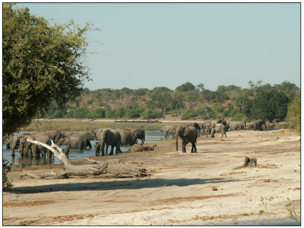
Figure 7.
The river’s edge in Chobe National Park, Botswana, is highly utilized by elephants and other species in the dry season. Extensive trampling results in scare vegetation and large amounts of bare soil, influencing Moving Standard Deviation Index (MSDI) values for this area. Photo credit: T. Fullman.

Our work also departed from previous studies by investigating the effect of changing the window size used in the standard deviation calculation. Previous studies used a 3 × 3-pixel window [42,44,123,124], and we added 5 × 5- and 7 × 7-pixel window sizes. Our analyses showed that while results were generally similar to smaller window sizes, a 7 × 7-pixel window resulted in lower model accuracy. Whether the 3 × 3- or 5 × 5-pixel window size offered better error reduction and explanatory power depended on the band or index used in the calculation. Interestingly, our evaluation showed that for the red band, a 5 × 5-pixel window size offered slightly better performance than the 3 × 3-pixel window used in previous studies. While it is unlikely that the general relationships highlighted in previous studies using a 3 × 3-pixel window on the red band would change if assessed with a 5 × 5-pixel window, our findings nonetheless suggest that future MSDI studies on the MODIS red band include a 5 × 5-pixel window along with the traditional 3 × 3.
While there is a statistically significant relationship between the MSDI and elephant utilization, the explanatory power of this relationship is relatively low, as indicated by the low R2 values (Table 1). Comparison between the ordinary and universal kriging models agree with this, showing similar R2 and RMSE values between models with and without the effects of the MSDI considered (Table 2). This suggests that while a relationship exists between MSDI values and elephant utilization, there may be other factors also influencing the MSDI. The presence of herbaceous vegetation may be one such factor. Vegetation indices, such as those used here in calculation of the MSDI, provide information about primary productivity but do not directly distinguish between reflectance from woody and herbaceous vegetation without additional information considering phenological shifts [46,86]. In light of this, the presence of herbaceous vegetation underneath a tree canopy may mask the changes in woody vegetation structure in which we are interested. This is likely another reason why the edge of the Chobe River, where both woody and herbaceous cover has typically been removed (Figure 7), showed such high MSDI values. The moderate spatial resolution of MODIS pixels at 250 m may also have influenced our results. The MSDI appears most suited to demonstrate coarse-scale trends reflecting increased heterogeneity due to patchy foraging across a landscape. Identifying finer-scale patches of high elephant use, however, may require imagery at finer spatial scales. Previous attempts to detect elephant impacts with remotely sensed methods have often used finer-scale imagery [125,126] or aerial photography [64,120]. While Scan Line Corrector issues with the Landsat 7 ETM+ satellite prevented evaluation of the MSDI using Landsat imagery, there is hope that with the newly launched Landsat 8 satellite, such analyses may be possible in the future. The cost of such finer-scale analyses will likely be in the extent that they can be generalized to inform regional management. Because of the importance of managing elephants not just in Chobe but across the entire Kavango-Zambezi Transfrontier Conservation Area, methods should ideally be developed that link findings from finer resolution images with coarser images like MODIS to provide information on regional patterns. In the meantime, while the MSDI provides information about elephant utilization, it does not seem to have a strong enough pattern to be effective for monitoring elephant impacts.
5. Conclusions
The United Nations Environment Programme (UNEP) recently released a policy brief on ecosystem management in Africa, which emphasizes the importance of maintaining healthy ecosystems for human well-being [127]. The brief points out that gaps in knowledge are one of the greatest impediments to developing an ecosystems approach to development and stresses the need for research and monitoring of ecological systems to enhance management decision making. Techniques to monitor agents of land cover change, such as elephants, using remote sensing can provide this much-needed information. A remotely-sensed measure of vegetation change due to elephants will allow a direct evaluation of how growing elephant densities over time result in altered levels of impact, a key concern for management [20]. It will also allow assessment of elephant impacts in places that have limited access for studies on the ground (such as Angola in the recent past).
We undertook the quantitative assessment of the Moving Standard Deviation Index (MSDI) called for by Robinson et al. [60]. Our findings confirm that at coarse scales there is a positive relationship between the MSDI and elephant utilization. At finer scales, however, we found that MSDI values are negatively related to elephant utilization of vegetation. This appears to be due to differences in within-patch and between-patch effects of elephants. While the patchiness of elephant utilization increases overall landscape heterogeneity, there may be a homogenizing effect of elephant herbivory at finer spatial scales. Although the relationship between the MSDI and elephant utilization is significant, the low explanatory power of our models suggests the MSDI may not be an effective means for distinguishing elephant-modified vegetation in Chobe National Park. It is unclear whether similar trends will hold for other systems with different types of vegetation. It would be interesting to see whether the MSDI is more effective at distinguishing elephant impacts in areas of higher soil nutrients, such as East Africa, as well as in succulent thicket ecosystems of South Africa, where elephant impacts are likely to result in vegetation removal, rather than coppice regrowth [24]. While the MSDI does not fully capture elephant utilization patterns, the potential value of remote assessment for informing management decisions of elephants and their impacts across Africa argues for its continued development.
Acknowledgments
Funding for this project was provided by NASA Project NNX09AI25G: Understanding and predicting the impact of climate variability and climate change on land use and land cover change via socio-economic institutions in Southern Africa, the Cleveland Metroparks Zoo and Cleveland Zoological Society, the National Science Foundation under Grant No. 0801544 in the Quantitative Spatial Ecology, Evolution and Environment IGERT Program at the University of Florida, and Idea Wild. The authors wish to thank K. Tjinjeka for assistance with fieldwork and for invaluable help in plant identification and B. Child for use of a field vehicle. Comments from J. Southworth, B. Child, E. Holmes, and three anonymous reviewers greatly improved the manuscript. P. Waylen provided T.J.F. with time for analysis and writing of the manuscript. Finally, thanks to the Botswana Department of Wildlife and National Parks for providing permission and support for this project.
Author Contributions
T.J.F. developed the study design, collected the field data and performed the analysis. E.L.B. prepared the remote sensing imagery and calculated the vegetation indices. Both authors contributed to the writing of the manuscript.
Conflicts of Interest
The authors declare no conflict of interest.
References
- Scholes, R.J.; Archer, S.R. Tree-grass interactions in Savannas. Annu. Rev. Ecol. Syst. 1997, 28, 517–544. [Google Scholar] [CrossRef]
- Sankaran, M.; Hanan, N.P.; Scholes, R.J.; Ratnam, J.; Augustine, D.J.; Cade, B.S.; Gignoux, J.; Higgins, S.I.; Le Roux, X.; Ludwig, F.; et al. Determinants of woody cover in African savannas. Nature 2005, 438, 846–849. [Google Scholar] [CrossRef]
- Skarpe, C. Dynamics of savanna ecosystems. J. Veg. Sci. 1992, 3, 293–300. [Google Scholar] [CrossRef]
- Loarie, S.R.; van Aarde, R.J.; Pimm, S.L. Elephant seasonal vegetation preferences across dry and wet savannas. Biol. Conserv. 2009, 142, 3099–3107. [Google Scholar] [CrossRef]
- Weltzin, J.F.; Coughenour, M.B. Savanna tree influence on understory vegetation and soil nutrients in northwestern Kenya. J. Veg. Sci. 1990, 1, 325–334. [Google Scholar] [CrossRef]
- Belsky, A.J. Influences of trees on savanna productivity: Tests of shade, nutrients, and tree-grass competition. Ecology 1994, 75, 922–932. [Google Scholar] [CrossRef]
- Sala, O.E.; Chapin, F.S., III; Armesto, J.J.; Berlow, E.; Bloomfield, J.; Dirzo, R.; Huber-Sanwald, E.; Huenneke, L.F.; Jackson, R.B.; Kinzig, A.; et al. Global biodiversity scenarios for the year 2100. Science 2000, 287, 1770–1774. [Google Scholar] [CrossRef]
- Desanker, P.V.; Justice, C.O. Africa and global climate change: Critical issues and suggestions for further research and integrated assessment modeling. Clim. Res. 2001, 17, 93–103. [Google Scholar] [CrossRef]
- Bell, R.H.V. The Effect of Soil Nutrient Availability on Community Structure in African Ecosystems. In Ecology of Tropical Savannas; Huntley, B.J., Walker, B.H., Eds.; Springer-Verlag: Berlin, Germany, 1982; pp. 193–216. [Google Scholar]
- Olff, H.; Ritchie, M.E.; Prins, H.H.T. Global environmental controls of diversity in large herbivores. Nature 2002, 415, 901–904. [Google Scholar] [CrossRef]
- Staver, A.C.; Archibald, S.; Levin, S.A. The global extent and determinants of savanna and forest as alternative biome states. Science 2011, 334, 230–232. [Google Scholar] [CrossRef]
- Staver, A.C.; Archibald, S.; Levin, S.A. Tree cover in Sub-Saharan Africa: Rainfall and fire constrain forest and savanna as alternative stable states. Ecology 2011, 92, 1063–1072. [Google Scholar] [CrossRef]
- Turner, B.L.; Skole, D.; Sanderson, S.; Fischer, G.; Fresco, L.; Leemans, R. Land-Use and Land-Cover Change. Science/Research Plan; IGBP Report No. 35 and HDP Report No. 7; International Geosphere-Biosphere Programme/Human Dimensions of Global Environmental Change Programme: Stockholm, Sweden/Geneva, Switzerland, 1995. [Google Scholar]
- Geist, H.J.; Lambin, E.F.; Rindfuss, R.R. Land Use and Land Cover Change. In Land-Use and Land-Cover Change: Local Processes and Global Impacts; Springer: New York, NY, USA, 2006; pp. 1–8. [Google Scholar]
- Cumming, D.H. The Influence of Large Herbivores on Savanna Structure in Africa. In Ecology of Tropical Savannas; Huntley, B.J., Walker, B.H., Eds.; Springer-Verlag: Berlin, Germany, 1982; pp. 217–245. [Google Scholar]
- Beuchner, H.K.; Dawkins, H.C. Vegetation change induced by elephants and fire in Murchison Falls National Park, Uganda. Ecology 1961, 42, 752–766. [Google Scholar] [CrossRef]
- Laws, R.M. Elephants as agents of habitat and landscape change in East Africa. Oikos 1970, 21, 1–15. [Google Scholar]
- Barnes, R.F.W. Effects of elephant browsing on woodlands in a Tanzanian National Park: Measurements, models and management. J. Appl. Ecol. 1983, 20, 521–540. [Google Scholar] [CrossRef]
- Goheen, J.R.; Keesing, F.; Allan, B.; Ogada, D.; Ostfeld, R. Net effects of large mammals on Acacia seedling survival in an African savanna. Ecology 2004, 85, 1555–1561. [Google Scholar] [CrossRef]
- Kerley, G.I.H.; Landman, M.; Kruger, L.; Owen-Smith, N.; Balfour, D.; de Boer, W.; Gaylard, A.; Lindsay, K.; Slotow, R. Effects of Elephants on Ecosystems and Biodiversity. In Elephant Management: A Scientific Assessment of South Africa; Scholes, R.J., Mennell, K.G., Eds.; Witwatersrand University Press: Johannesburg, South Africa, 2008; pp. 146–205. [Google Scholar]
- Paine, R.T. A note on trophic complexity and community stability. Am. Nat. 1969, 103, 91–93. [Google Scholar]
- Holdo, R.M. Elephants, fire, and frost can determine community structure and composition in Kalahari woodlands. Ecol. Appl. 2007, 17, 558–568. [Google Scholar] [CrossRef]
- Norton-Griffiths, M. The Influence of Grazing, Browsing, and Fire on the Vegetation Dynamics of the Serengeti. In Serengeti: Dynamics of an Ecosystem; Sinclair, A.R.E., Norton-Griffiths, M., Eds.; University of Chicago Press: Chicago, IL, USA, 1979; pp. 310–351. [Google Scholar]
- Kerley, G.I.H.; Landman, M. The impacts of elephants on biodiversity in the Eastern Cape subtropical thickets. S. Afr. J. Sci. 2006, 102, 395–402. [Google Scholar]
- United Nations Environment Programme (UNEP); Convention on International Trade in Endangered Species of Wild Fauna and Flora (CITES); International Union for Conservation of Nature (IUCN); TRAFFIC. Elephants in the Dust—The African Elephant Crisis; A Rapid Response Assessment; United Nations Environment Programme/GRID-Arendal. Available online: http://www.grida.no/publications/rr/elephants/ (accessed on 22 April 2013).
- Glover, J. The elephant problem at Tsavo. Afr. J. Ecol. 1963, 1, 30–39. [Google Scholar] [CrossRef]
- Barnes, R.F.W. The elephant problem in Ruaha National Park, Tanzania. Biol. Conserv. 1983, 26, 127–148. [Google Scholar] [CrossRef]
- Valeix, M.; Fritz, H.; Dubois, S.; Kanengoni, K.; Alleaume, S.; Said, S. Vegetation structure and ungulate abundance over a period of increasing elephant abundance in Hwange National Park, Zimbabwe. J. Trop. Ecol. 2007, 23, 87–93. [Google Scholar] [CrossRef]
- Blanc, J.J.; Barnes, R.F.W.; Craig, G.C.; Dublin, H.T.; Thouless, C.R.; Douglas-Hamilton, I.; Hart, J.A. African Elephant Status Report 2007: An Update from the African Elephant Database; Occasional Paper Series of the IUCN Species Survival Commission, No. 33; IUCN/SSC African Elephant Specialist Group, International Union for Conservation of Nature (IUCN): Gland, Switzerland, 2007. [Google Scholar]
- Blignaut, J.; de Wit, M.; Barnes, J. The Economic Value of Elephants. In Elephant Management: A Scientific Assessment of South Africa; Scholes, R.J., Mennell, K.G., Eds.; Witwatersrand University Press: Johannesburg, South Africa, 2008; pp. 446–476. [Google Scholar]
- Thouless, C.R. Conflict between humans and elephants on private land in northern Kenya. Oryx 1994, 28, 119–127. [Google Scholar] [CrossRef]
- Hoare, R.E. Determinants of human-elephant conflict in a land-use mosaic. J. Appl. Ecol. 1999, 36, 689–700. [Google Scholar] [CrossRef]
- Hoare, R.E. African elephants and humans in conflict: The outlook for co-existence. Oryx 2000, 34, 34–38. [Google Scholar]
- Prins, H.H.T. Chapter 6/7; Competition for Food/Patch Selection Predators and Grazing by Rule of Thumb. In Ecology and Behaviour of the African Buffalo: Social Inequality and Decision Making; Chapman & Hall: London, UK, 1996; pp. 154–203. [Google Scholar]
- Skarpe, C.; Aarrestad, P.A.; Andreassen, H.P.; Dhillion, S.S.; Dimakatso, T.; du Toit, J.T.; Duncan; Halley, J.; Hytteborn, H.; Makhabu, S.; Marl, M.; et al. The return of the giants: Ecological effects of an increasing elephant population. Ambio 2004, 33, 276–282. [Google Scholar]
- Inamdar, A. The Ecological Consequences of Elephant Depletion. Ph.D. Thesis, University of Cambridge, Cambridge, UK, 1996. [Google Scholar]
- Dipotso, F.M.; Skarpe, C.; Kelaeditse, L.; Ramotadima, M. Chobe bushbuck in an elephant-impacted habitat along the Chobe River. Afr. Zool. 2007, 42, 261–267. [Google Scholar] [CrossRef]
- Western, D.; Gichohi, H. Segregation effects and the impoverishment of savanna parks: The case for ecosystem viability analysis. Afr. J. Ecol. 1993, 31, 269–281. [Google Scholar] [CrossRef]
- Rutina, L.P.; Moe, S.R.; Swenson, J.E. Elephant Loxodonta africana driven woodland conversion to shrubland improves dry-season browse availability for impalas Aepyceros melampus. Wildl. Biol. 2005, 11, 207–213. [Google Scholar] [CrossRef]
- Makhabu, S.W.; Skarpe, C.; Hytteborn, H. Elephant impact on shoot distribution on trees and on rebrowsing by smaller browsers. Acta Oecol. 2006, 30, 136–146. [Google Scholar] [CrossRef]
- Valeix, M.; Fritz, H.; Sabatier, R.; Murindagomo, F.; Cumming, D.; Duncan, P. Elephant-induced structural changes in the vegetation and habitat selection by large herbivores in an African savanna. Biol. Conserv. 2011, 144, 902–912. [Google Scholar] [CrossRef]
- Tanser, F.C.; Palmer, A.R. The application of a remotely-sensed diversity index to monitor degradation patterns in a semi-arid, heterogeneous, South African landscape. J. Arid Environ. 1999, 43, 477–484. [Google Scholar] [CrossRef]
- Schlesinger, W.H.; Reynolds, J.F.; Cunningham, G.L.; Huenneke, L.F.; Jarrell, W.M.; Virginia, R.A.; Whitford, W.G. Biological feedbacks in global desertification. Science 1990, 247, 1043–1048. [Google Scholar]
- Jafari, R.; Lewis, M.M.; Ostendorf, B. An image-based diversity index for assessing land degredation in an arid environment in South Australia. J. Arid Environ. 2008, 72, 1282–1293. [Google Scholar] [CrossRef]
- Pickup, G.; Chewings, V.H. Forecasting patterns of erosion in arid lands from Landsat MSS data. Int. J. Remote Sens. 1988, 9, 69–84. [Google Scholar] [CrossRef]
- Jensen, J.R. Chapter 8: Image Enhancement. In Introductory Digital Image Processing: A Remote Sensing Perspective, 3rd ed.; Pearson Education, Inc.: Upper Saddle River, NJ, USA, 2005; pp. 301–322. [Google Scholar]
- Knipling, E.B. Physical and physiological basis for the reflectance of visible and near-infrared radiation from vegetation. Remote Sens. Environ. 1970, 1, 155–159. [Google Scholar] [CrossRef]
- Tucker, C.J. Red and photographic infrared linear combinations for monitoring vegetation. Remote Sens. Environ. 1979, 8, 127–150. [Google Scholar] [CrossRef]
- Chavez, P.S., Jr.; MacKinnon, D.J. Automatic detection of vegetation changes in the southwestern United States using remotely sensed images. Photogramm. Eng. Remote Sens. 1994, 60, 571–583. [Google Scholar]
- Horler, D.N.; Dockray, M.; Barber, J. The red edge of plant leaf reflectance. Int. J. Remote Sens. 1983, 4, 273–288. [Google Scholar] [CrossRef]
- Huete, A.R. A soil-adjusted vegetation index (SAVI). Remote Sens. Environ. 1988, 25, 295–309. [Google Scholar]
- Huete, A.R.; Liu, H.Q.; Batchily, K.; van Leeuwen, W. A comparison of vegetation indices over a global set of TM images for EOS-MODIS. Remote Sens. Environ. 1997, 59, 440–451. [Google Scholar]
- Huete, A.R.; Didan, K.; Miura, T.; Rodriguez, E.P.; Gao, X.; Ferreira, L.G. Overview of the radiometric and biophysical performance of the MODIS vegetation indices. Remote Sens. Environ. 2002, 83, 195–213. [Google Scholar]
- Loveland, T.R.; Reed, B.C.; Brown, J.L.; Ohlen, D.O.; Zhu, Z.; Yang, L.; Merchant, J.W. Development of a global land cover characteristics database and IGBP DISCover from 1 km AVHRR data. Int. J. Remote Sens. 2000, 21, 1303–1330. [Google Scholar] [CrossRef]
- Ecosystem Function in Savannas: Measurement and Modeling at Landscape to Global Scales; Hill, M.; Hanan, N.P. (Eds.) CRC Press: Boca Raton, FL, USA, 2011.
- Archibald, S.; Scholes, R.J. Leaf green-up in a semi-arid African savanna—Separating tree and grass responses to environmental cues. J. Veg. Sci. 2007, 18, 583–594. [Google Scholar]
- Fensholt, R.; Sandholt, I.; Stisen, S. Evaluating MODIS, MERIS, and VEGETATION vegetation indices using in situ measurements in a semiarid environment. IEEE Trans. Geosci. Remote Sens. 2006, 44, 1774–1786. [Google Scholar] [CrossRef]
- Duffy, J.P.; Pettorelli, N. Exploring the relationship between NDVI and African elephant population density in protected areas. Afr. J. Ecol. 2013, 50, 455–463. [Google Scholar] [CrossRef]
- Nellis, M.D.; Lulla, K.; Briggs, J.M.; Bussing, C.E. Interfacing geographic information systems and space shuttle photography for monitoring elephant impact in Botswana. Pap. Proc. Appl. Geogr. Conf. 1990, 13, 10–15. [Google Scholar]
- Robinson, J.A.; Lulla, K.P.; Kashiwagi, M.; Suzuki, M.; Nellis, M.D.; Bussing, C.E.; Long, W.J.L.; McKenzie, L.J. Conservation applications of astronaut photographs of earth: Tidal-flat loss (Japan), elephant effects on vegetation (Botswana), and seagrass and mangrove monitoring (Australia). Conserv. Biol. 2001, 15, 876–884. [Google Scholar] [CrossRef]
- Campbell, A.C. The national park and reserve system in Botswana. Biol. Conserv. 1973, 5, 7–14. [Google Scholar] [CrossRef]
- Cushman, S.A.; Chase, M.; Griffin, C. Elephants in space and time. Oikos 2005, 109, 331–341. [Google Scholar] [CrossRef]
- Child, G. Wildlife utilization and management in Botswana. Biol. Conserv. 1970, 3, 18–22. [Google Scholar] [CrossRef]
- Mosugelo, D.K.; Moe, S.R.; Ringrose, S.; Nellemann, C. Vegetation changes during a 36-year period in northern Chobe National Park, Botswana. Afr. J. Ecol. 2002, 40, 232–240. [Google Scholar] [CrossRef]
- Fullman, T.J.; Child, B. Water distribution at local and landscape scales affects tree utilization by elephants in Chobe National Park, Botswana. Afr. J. Ecol. 2013, 51, 235–243. [Google Scholar] [CrossRef]
- Reich, P.B.; Borchert, R. Water stress and tree phenology in a tropical dry forest in the lowlands of Costa Rica. J. Ecol. 1984, 72, 61–74. [Google Scholar] [CrossRef]
- Borchert, R. Soil and stem water storage determine phenology and distribution of tropical dry forest trees. Ecology 1994, 75, 1437–1449. [Google Scholar] [CrossRef]
- Borchert, R. Climatic periodicity, phenology and cambium activity in dry forest trees. IAWA J. 1999, 20, 239–247. [Google Scholar]
- Shisanya, C.A.; Recha, C.; Anyamba, A. rainfall variability and its impacts on NDVI in arid and semi-arid lands of Kenya. Int. J. Geosci. 2011, 2, 36–47. [Google Scholar] [CrossRef]
- Food and Agriculture Organization of the United Nations (FAO); International Institute for Applied Systems Analysis (IIASA); International Soil Reference and Information Centre (ISRIC); Institute of Soil Science-Chinese Academy of Sciences (ISSCAS); Joint Research Centre of the European Commission (JRC). Harmonized World Soil Database (Version 1.2); FAO/IIASA: Rome, Italy/Laxenburg, Austria, 2012. [Google Scholar]
- Child, G. An Ecological Survey of Northeastern Botswana; FAO #TA2563; Food and Agriculture Organization of the United Nations (FAO): Rome, Italy, 1968. [Google Scholar]
- Herremans, M.; Herremans-Tonnoeyr, D. Land use and the conservation status of raptors in Botswana. Biol. Conserv. 2000, 94, 31–41. [Google Scholar] [CrossRef]
- Gibson, D.S.C.; Craig, G.C.; Masogo, R.M. Trends of the elephant population in northern Botswana from aerial survey data. Pachyderm 1998, 25, 14–27. [Google Scholar]
- Barnes, M.E. Effects of large herbivores and fire on the regeneration of Acacia erioloba woodlands in Chobe National Park, Botswana. Afr. J. Ecol. 2001, 39, 340–350. [Google Scholar] [CrossRef]
- Moe, S.R.; Rutina, L.P.; Hytteborn, H.; du Toit, J.T. What controls woodland regeneration after elephants have killed the big trees? J. Appl. Ecol. 2009, 46, 223–230. [Google Scholar] [CrossRef]
- Peace Parks Foundation: The Global Solution. Available online: http://www.peaceparks.org/ (accessed on 17 September 2013).
- Kavango-Zambezi Transfrontier Conservation Area. Available online: http://www.kavangozambezi.org/ (accessed on 17 September 2013).
- Van Aarde, R.J.; Jackson, T.P.; Ferreira, S.M. Conservation science and elephant management in southern Africa. S. Afr. J. Sci. 2006, 102, 385–388. [Google Scholar]
- Van Aarde, R.J.; Jackson, T.P. Megaparks for meapopulations: Addressing the causes of locally high elephant numbers in southern Africa. Biol. Conserv. 2007, 134, 289–297. [Google Scholar] [CrossRef]
- USGS. LP DAAC Data Pool. Available online: https://lpdaac.usgs.gov/get_data/data_pool (accessed on 11 September 2012).
- USGS. LP DAAC MODIS Reprojection Tool. Available online: https://lpdaac.usgs.gov/tools/modis_reprojection_tool (accessed on 11 September 2012).
- Graetz, R.D.; Pech, R.R.; Davis, A.W. The assessment and monitoring of sparsely vegetated rangelands using calibrated Landsat data. Int. J. Remote Sens. 1988, 9, 1201–1222. [Google Scholar] [CrossRef]
- McNaughton, S.J.; Oesterheld, M.; Frank, D.A.; Williams, K.J. Ecosystem-level patterns of primary productivity and herbivory in terrestrial habitats. Nature 1989, 341, 142–144. [Google Scholar] [CrossRef]
- Chapin, F.S., III; Bret-Harte, M.S.; Hobbie, S.A.; Zhong, H. Plant functional types as predictors of transient responses of arctic vegetation to global change. J. Veg. Sci. 1996, 7, 347–358. [Google Scholar] [CrossRef]
- Holm, A.M.; Watson, I.W.; Loneragan, W.A.; Adams, M.A. Loss of patch-scale heterogeneity on primary productivity and rainfall-use efficiency in Western Australia. Basic Appl. Ecol. 2003, 4, 569–578. [Google Scholar] [CrossRef]
- Glenn, E.P.; Huete, A.R.; Nagler, P.L.; Nelson, S.G. Relationship between remotely-sensed vegetation indices, canopy attributes and plant physiological processes: What vegetation indices can and cannot tell us about the landscape. Sensors 2008, 8, 2136–2160. [Google Scholar] [CrossRef]
- Huete, A.; Justice, C.; van Leeuwen, W. MODIS Vegetation Index (MOD 13): Algorithm Theoretical Basis Document. Version 3; USGS Land Process Distributed Active Archive Center, 1999. Available online: http://modis.gsfc.nasa.gov/data/atbd/atbd_mod13.pdf (accessed on 4 December 2012).
- Pettorelli, N.; Ryan, S.; Mueller, T.; Bunnefeld, N.; Jędrzejewska, B.; Lima, M.; Kausrud, K. The Normalized Difference Vegetation Index (NDVI): Unforeseen successes in animal ecology. Clim. Res. 2011, 46, 15–27. [Google Scholar] [CrossRef]
- Huete, A.R.; Jackson, R.D. Suitability of spectral indices for evaluating vegetation characteristics on arid rangelands. Remote Sens. Environ. 1987, 23, 213–232. [Google Scholar] [CrossRef]
- Huete, A.R.; Jackson, R.D. Soil and atmosphere influences on the spectra of partial canopies. Remote Sens. Environ. 1988, 25, 89–105. [Google Scholar] [CrossRef]
- Qi, J.; Kerr, Y.; Chehbouni, A. External Factor Consideration in Vegetation Index Development. In Proceedings of the 6th International Symposium on Physical Measurements and Signatures in Remote Sensing, Val d’Isere, France, 17–21 January 1994; pp. 723–730.
- Hijmans, R.J.; van Etten, J. Raster: Geographic Data Analysis and Modeling, R Package Version 2.0-31; 2012. Available online: http://CRAN.R-project.org/package=raster (accessed on 27 March 2012).
- R Core Team. R: A Language and Environment for Statistical Computing; R Foundation for Statistical Computing: Vienna, Austria, 2012. Available online: http://www.R-project.org (accessed on 9 March 2012).
- Fullman, T.J. Spatial Dynamics of Elephant Impacts on Trees in Chobe National Park, Botswana. M.Sc. Thesis, University of Florida, Gainesville, FL, USA, 2009. [Google Scholar]
- Guldemond, R.; van Aarde, R. A meta-analysis of the impact of African elephants on savanna vegetation. J. Wildl. Manag. 2008, 72, 892–899. [Google Scholar]
- Young, T.P.; Palmer, T.M.; Gadd, M.E. Competition and compensation among cattle, zebras, and elephants in a semi-arid savanna in Laikipia, Kenya. Biol. Conserv. 2005, 122, 351–359. [Google Scholar] [CrossRef]
- Fuller, T.K. Do pellet counts index white-tailed deer numbers and population change? J. Wildl. Manag. 1991, 55, 393–396. [Google Scholar]
- Barnes, R.F.W. How reliable are dung counts for estimating elephant numbers? Afr. J. Ecol. 2001, 39, 1–9. [Google Scholar]
- Odén, A.; Wedel, H. Arguments for Fisher’s permutation test. Ann. Stat. 1975, 3, 518–520. [Google Scholar] [CrossRef]
- Ruxton, G.D. The unequal variance t-test is an underused alternative to Student’s t-test and the Mann-Whitney U test. Behav. Ecol. 2006, 17, 688–690. [Google Scholar] [CrossRef]
- Hijmans, R.J.; Phillips, S.; Leathwick, J.; Elith, J. Dismo: Species Distribution Modeling, R Package Version 0.7-23; 2012. Available online: http://CRAN.R-project.org/package=dismo (accessed on 9 March 2012).
- Nellemann, C.; Moe, S.R.; Rutina, L.P. Links between terrain characteristics and forage patterns of elephants (Loxodonta africana) in northern Botswana. J. Trop. Ecol. 2002, 18, 835–844. [Google Scholar]
- Moran, P.A.P. Notes on continuous stochastic phenomena. Biometrika 1950, 37, 17–23. [Google Scholar]
- Anselin, L. Local indicators of spatial association—LISA. Geogr. Anal. 1995, 27, 93–115. [Google Scholar] [CrossRef]
- Cliff, A.D.; Ord, J.K. Spatial Autocorrelation; Pion Limited: London, UK, 1973. [Google Scholar]
- Schabenberger, O.; Gotway, C.A. Statistical Methods for Spatial Data Analysis; Chapman & Hall/CRC: Boca Raton, FL, USA, 2005. [Google Scholar]
- Kissling, W.D.; Carl, G. Spatial autocorrelation and the selection of simultaneous autoregressive models. Glob. Ecol. Biogeogr. 2008, 17, 59–71. [Google Scholar]
- Chiang, C.-T.; Lian, I.-B.; Su, C.-C.; Tsai, K.-Y.; Lin, Y.-P.; Chang, T.-K. Spatiotemporal trends in oral cancer mortality and potential risks associated with heavy metal content in Taiwan soil. Int. J. Environ. Res. Public Health 2010, 7, 3916–3928. [Google Scholar] [CrossRef]
- Anselin, L.; Bera, A.K.; Florax, R.; Yoon, M.J. Simple diagnostic tests for spatial dependence. Reg. Sci. Urban Econ. 1996, 26, 77–104. [Google Scholar] [CrossRef]
- Bivand, R.; Altman, M.; Anselin, L.; Assuncao, R.; Berke, O.; Bernat, A.; Blanchet, G.; Blankmeyer, E.; Carvalho, M.; Christensen, B.; et al. Spdep: Spatial Dependence: Weighting Schemes, Statistics and Models, R Package Version 0.5-51; 2012. Available online: http://CRAN.R-project.org/package=spdep (accessed on 9 March 2012).
- Matheron, G. Principles of geostatistics. Econ. Geol. 1963, 58, 1246–1266. [Google Scholar] [CrossRef]
- Legendre, P.; Fortin, M.-J. Spatial pattern and ecological analysis. Vegetatio 1989, 80, 107–138. [Google Scholar] [CrossRef]
- Childés, J.-P.; Delfiner, P. Geostatistics: Modeling Spatial Uncertainty; Wiley: New York, NY, USA, 1999. [Google Scholar]
- Pebesma, E.J. Multivariable geostatistics in S: The gstat package. Comput. Geosci. 2004, 30, 683–691. [Google Scholar] [CrossRef]
- Davis, B.M. Uses and abuses of cross-validation in geostatistics. Math. Geol. 1987, 19, 241–248. [Google Scholar] [CrossRef]
- Bivand, R.S.; Pebesma, E.J.; Gómez-Rubio, V. Applied Spatial Data Analysis with R; Springer: New York, NY, USA, 2008. [Google Scholar]
- White, F. Vegetation of Africa—A Descriptive Memoir to Accompany the Unesco/AETFAT/UNSO Vegetation Map of Africa; Natural Resources Research Report XX; United Nation-Educational, Scientific and Cultural Organization: Paris, France, 1983; p. 356. [Google Scholar]
- Akaike, H. Information Theory and an Extension of the Maximum Likelihood Principle. In Second International Symposium on Information Theory; Petrov, B.N., Csaki, F., Eds.; Akademiai Kaido: Budapest, Hungary, 1973; pp. 267–281. [Google Scholar]
- Akaike, H. Prediction and Entropy. In A Celebration of Statistics; Atkinson, A.C., Fienberg, S.E., Eds.; Springer: New York, NY, USA, 1985; pp. 1–24. [Google Scholar]
- Teren, G.; Owen-Smith, N.; Erasmus, B.F.N. Structural and compositional riparian woodland change caused by extreme elephant impact in northern Botswana. S. Afr. J. Bot. 2011, 77, 560–561. [Google Scholar]
- Kalwij, J.M.; de Boer, W.F.; Mucina, L.; Prins, H.H.T.; Skarpe, C.; Winterbach, C. Tree cover and biomass increase in a southern African savanna despite growing elephant population. Ecol. Appl. 2010, 20, 222–233. [Google Scholar] [CrossRef]
- Teren, G.; Owen-Smith, N. Elephants and riparian woodland changes in the Linyanti region, northern Botswana. Pachyderm 2010, 47, 18–25. [Google Scholar]
- Tanser, F.; Palmer, A.R. Vegetation mapping of the Great Fish River basin, South Africa: Integrating spatial and multi-spectral remote sensing techniques. Appl. Veg. Sci. 2000, 3, 197–204. [Google Scholar] [CrossRef]
- Xu, D.; Kang, X.; Qiu, D.; Zhuang, D.; Pan, J. Quantitative assessment of desertification using landsat data on a regional scale—A case study in the Ordos Plateau, China. Sensors 2009, 9, 1738–1753. [Google Scholar] [CrossRef]
- Nellis, M.D.; Bussing, C.E. Spatial variation in elephant impact on the Zambezi teak forest in the Chobe National Park, Botswana. Geocarto Int. 1990, 2, 55–57. [Google Scholar] [CrossRef]
- Simms, C. The Utilisation of Satellite Images for the Detection of Elephant Induced Vegetation Change Patterns. M.Sc. Thesis, University of South Africa, Pretoria, South Africa, 2009. [Google Scholar]
- Munang, R.; Liu, J.; Chuku, C.A.; Codjoe, S.; Dovie, D.; Mkwambisi, D.D.; Rivington, M. Putting Ecosystem Management in the Vision of Africa’s Development: Towards a sustainable Green Economy. In UNEP Policy Series on Ecosystem Management; United Nations Environment Programme: Nairobi, Kenya, 2011. [Google Scholar]
© 2014 by the authors; licensee MDPI, Basel, Switzerland. This article is an open access article distributed under the terms and conditions of the Creative Commons Attribution license (http://creativecommons.org/licenses/by/3.0/).