Historical and Contemporary Geographic Data Reveal Complex Spatial and Temporal Responses of Vegetation to Climate and Land Stewardship


Abstract
:1. Introduction
1.1. Historical Data
1.2. Fusion of Historical and Contemporary Data
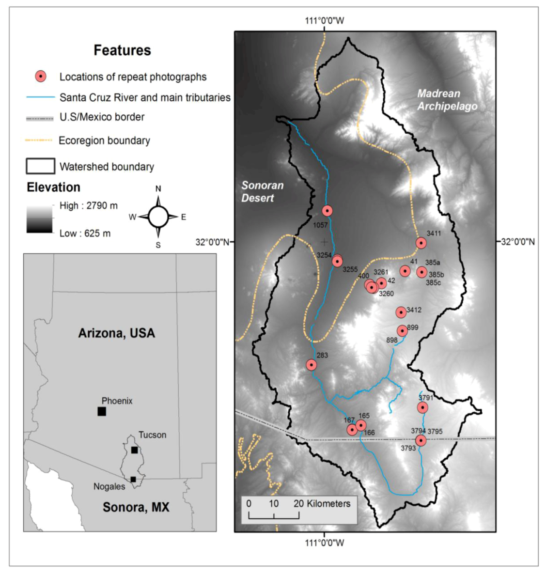
1.3. Study Area

1.4. Materials and Methods
1.4.1. Multitemporal Land Cover

| Date | Land Cover Maps | Deciduous Forest | Grassland | |||
| Overall Accuracy (%) | Kappa | Users (%) | Producers (%) | Users (%) | Producers (%) | |
| 1979 | 84.8 | 0.835 | 90 | 85 | 78 | 89 |
| 1989 | 84.3 | 0.829 | 92 | 80 | 74 | 65 |
| 1999 | 81.8 | 0.802 | 78 | 81 | 86 | 86 |
| 2009 | 86.5 | 0.854 | 86 | 84 | 83 | 80 |
1.4.2. Post-Classification Change Detection
1.4.3. Repeat Photography
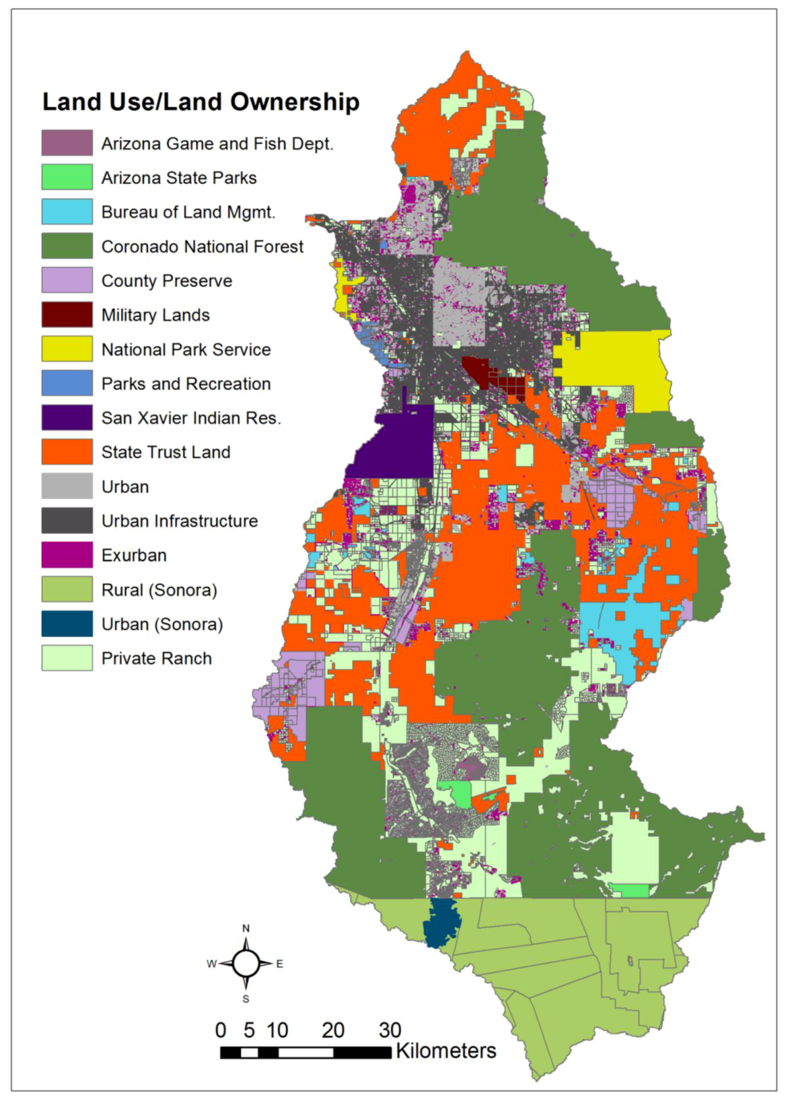
1.4.4. Land Ownership and Ecoregion
| Land Use/Land Ownership | Description | Area (ha) | # of units | Mean (ha) |
|---|---|---|---|---|
| AZ Game and Fish Dept. | Managed by Arizona Game and Fish Dept. | 1,498 | 67 | 22.4 |
| AZ State Parks | Parklands managed by the State of Arizona. | 3,819 | 56 | 68.2 |
| Bureau of Land Mgmt. | Uses range from ranching to conservation. | 21,359 | 276 | 65.2 |
| Coronado National Forest | Managed by US National Forest Service. | 190,175 | 466 | 451.9 |
| County Preserve | Ranches and open space purchased for conservation. | 24,495 | 440 | 49.1 |
| Exurban | 1.7–6.7 ha. Uses include rural homesteads and guest ranches. | 33,882 | 11,754 | 2.9 |
| Military Lands | Department of Defense lands. | 4,351 | 59 | 65.9 |
| National Park Service | Managed by US National Park Service. | 23,332 | 3 | 507.4 |
| Parks and Recreation | Parklands managed by Pima and Santa Cruz counties. | 2,799 | 142 | 18.6 |
| Private Ranch | > 6.8 ha. Uses include cattle grazing and agriculture. | 175,475 | 3,987 | 39.5 |
| Rural (Sonora) | Communal ejido lands. Uses include grazing and agriculture. | 98,714 | 27 | 3,655.0 |
| San Xavier Indian Res. | Managed by the Tohono O'odham Nation. | 15,447 | 8 | 1,931.0 |
| State Trust Land | AZ undeveloped lands auctioned to provide Trust revenue. | 175,685 | 641 | 193.6 |
| Urban | < 1.7 ha. High density urban to suburban ranch uses. | 53,946 | 127,737 | 0.4 |
| Urban (Sonora) | High density urban lands in and around Nogales, Sonora. | 3,749 | 143 | 26.2 |
| Urban Infrastructure | Road networks, freeways, airports. | 32,406 | 16 | 3,150.7 |

2. Results
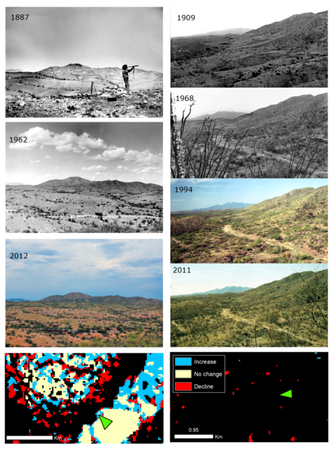
2.1. Photographic Evidence of Change, Pre-Land Cover (1887–1978)
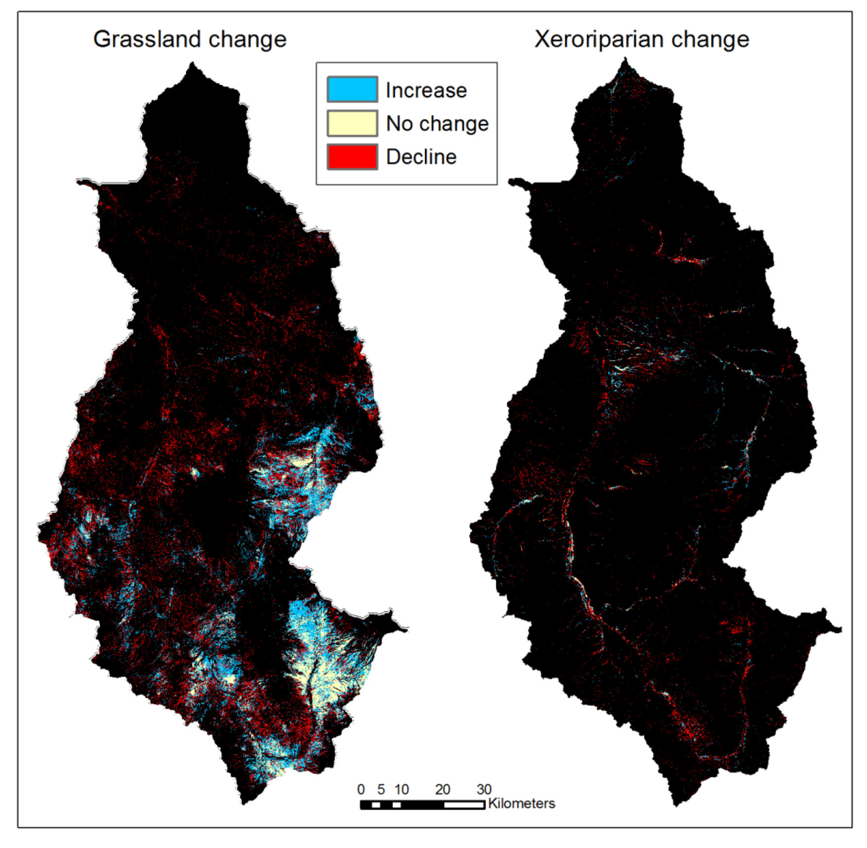
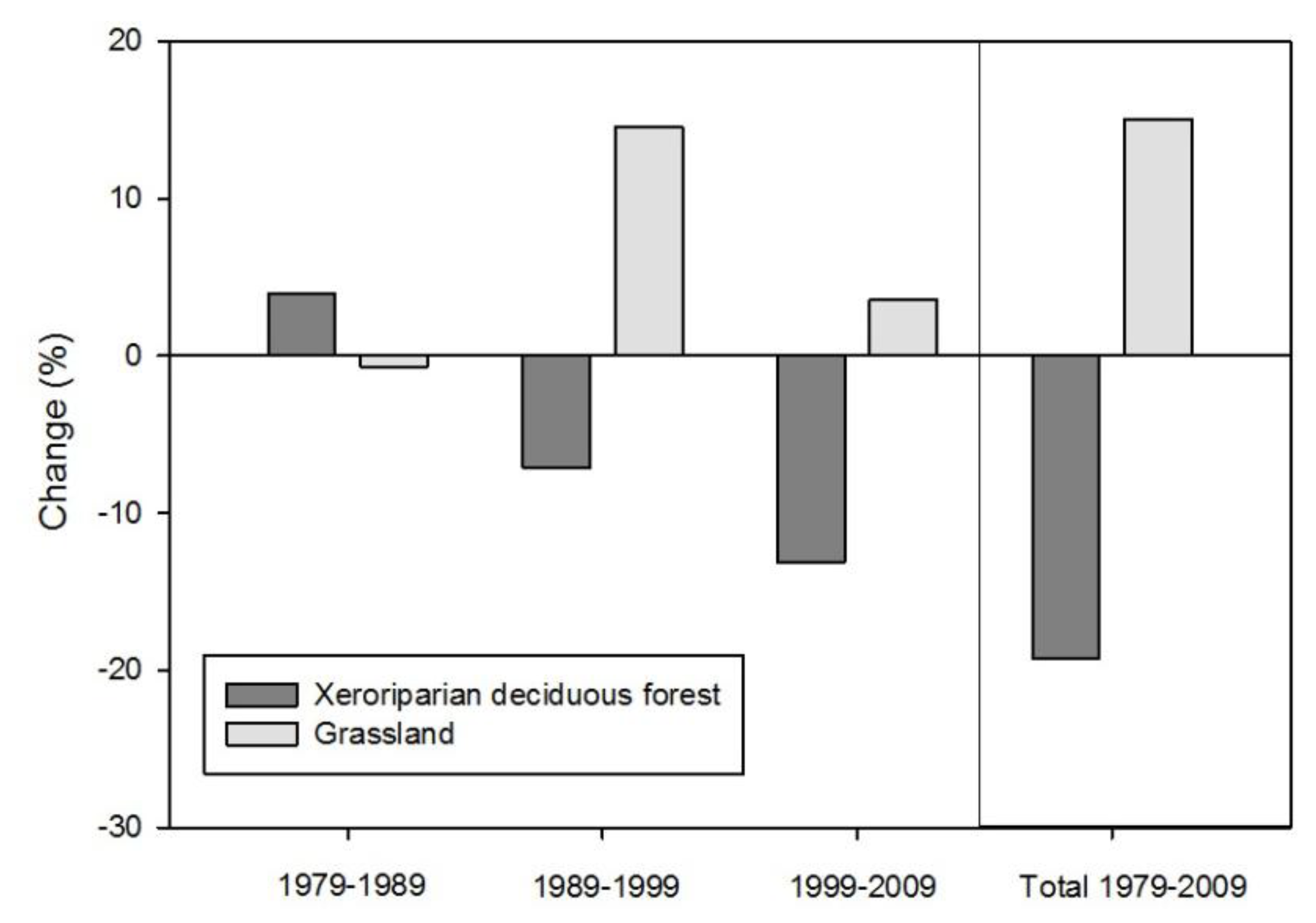
2.2. Broad Landscape-Scale Changes, 1979–2009
| Location | Stake # | 1st Date | Photos (n) | Land Use/Land Ownership | Vegetation | Historical ∆ | Recent ∆ | Mapped ∆* |
|---|---|---|---|---|---|---|---|---|
| Santa Cruz | 165 | 1887 | 4 | Private Ranch | Grassland | Grass (-) | Grass (+) | Grass (+) |
| Nogales | 166 | 1887 | 4 | Private Ranch | Grassland | Woody (+) | Woody (=) | Woody (=) |
| Nogales | 167 | 1887 | 4 | Private Ranch | Grassland | Woody (+) | Woody (=) | Woody (=) |
| Helvetia | 400 | 1909 | 4 | State Trust Land | Grassland | Woody (+) | Woody (=) | Woody (=) |
| Lopez Exclosure | 898 | 1977 | 4 | Coronado National Forest | Grassland | Grass (=) | Grass (=) | Grass (=) |
| Lopez Exclosure | 899 | 1977 | 4 | Private | Grassland | Grass (=) | Grass (-) | Grass (-) |
| Santa Rita Range | 3255 | 1978 | 2 | Coronado National Forest | Grassland | Grass (=) | Grass (=) | Grass (=) |
| Santa Rita Range | 3260 | 1978 | 2 | Coronado National Forest | Grassland | Grass (=) | Grass (=) | Grass (=) |
| Santa Rita Range | 3261 | 1978 | 3 | Coronado National Forest | Grassland | Grass (=) | Grass (=) | Grass (=) |
| Santa Rita | 3412 | 1955 | 3 | Private | Grassland | Grass (-) | Grass (-) | Grass (-) |
| San Rafael Valley | 3791 | 1932 | 3 | Private | Grassland | Grass (=) | Grass (=) | Grass (=) |
| Lochiel - MEX | 3793 | 1930 | 3 | Private | Grassland | Grass (-) | Grass (=) | Grass (=) |
| Lochiel - USA | 3793 | 1930 | 3 | Private | Grassland | Grass (=) | Grass (=) | Grass (=) |
| Total Wreck Mine | 358a | 1909 | 3 | State Trust Land | Grassland | Woody (+) | (=) | (=) |
| Total Wreck Mine | 385b | 1909 | 3 | State Trust Land | Grassland | Woody (+) | (=) | (=) |
| Total Wreck Mine | 385c | 1909 | 3 | State Trust Land | Grassland | Woody (+) | (=) | (=) |
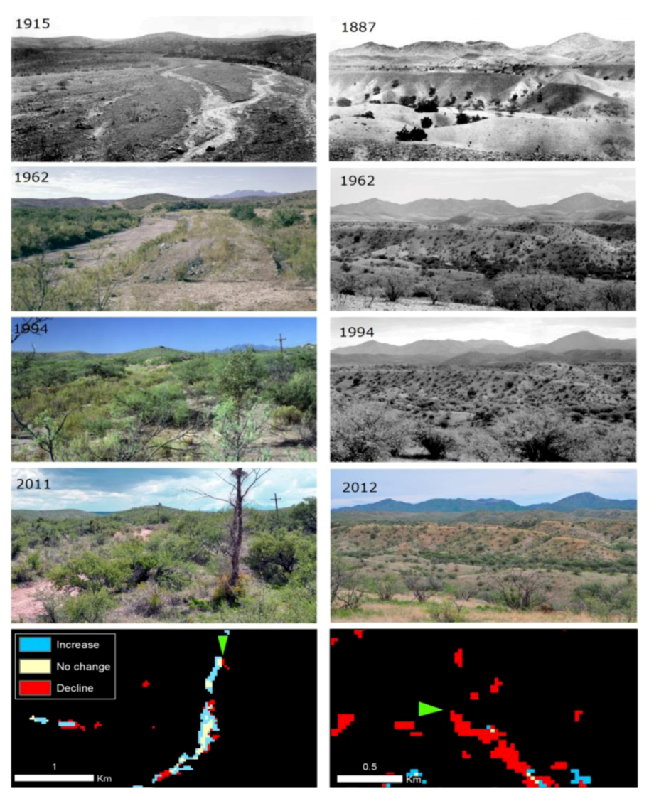
| Davidson Creek | 41 | 1915 | 4 | Exurban | Xeroriparian | Woody (+) | Woody (-) | Woody (-) |
| Rosemont Mine | 42 | 1910 | 4 | Coronado National Forest | Xeroriparian | Woody (+) | Woody (-) | Woody (=) |
| Yerba Buena | 165 | 1887 | 4 | Private Ranch | Xeroriparian | Woody (+) | Woody (-) | Woody (-) |
| Tumacacori | 283 | 1890 | 3 | National Park Service | Xeroriparian | Woody (+) | Woody (=) | Woody (=) |
| Santa Rita Range | 3254 | 1978 | 3 | Coronado National Forest | Xeroriparian | Woody (=) | Woody (+) | Woody (+) |
| San Rafael Valley | 3791 | 1932 | 3 | Private | Xeroriparian | Woody (+) | Woody (-) | Woody (-) |
| Lochiel | 3793 | 1930 | 3 | Private | Xeroriparian | Woody (+) | Woody (-) | Woody (-) |
| Martinez Hill | 1057 | 1912 | 4 | San Xavier Indian Res. | Xeroriparian | Woody (-) | Woody (-) | Woody (-) |
| Cienega Creek | 3411 | 1880 | 3 | County Preserve | Xeroriparian | Woody (+) | Woody (=) | Woody (=) |
| Cover Change | 1979–1989 | 1989–1999 | 1999–2009 |
|---|---|---|---|
| Shrubland to grassland | 39,436 | 31,602 | 32,582 |
| Grassland to shrubland | 39,941 | 24,474 | 30,661 |
| Grassland to developed | 1,657 | 493 | 873 |
| Grassland to barren | 724 | 392 | 1,029 |
| Net change grassland | −2,886 | 6,243 | 19 |
| Shrubland to xeroriparian | 5,317 | 2,620 | 2,434 |
| Xeroriparian to shrubland | 4,059 | 3,494 | 2,760 |
| Xeroriparian to developed | 810 | 1,058 | 800 |
| Xeroriparian to barren | 241 | 155 | 193 |
| Net change xeroriparian | 207 | −2,086 | −1319 |
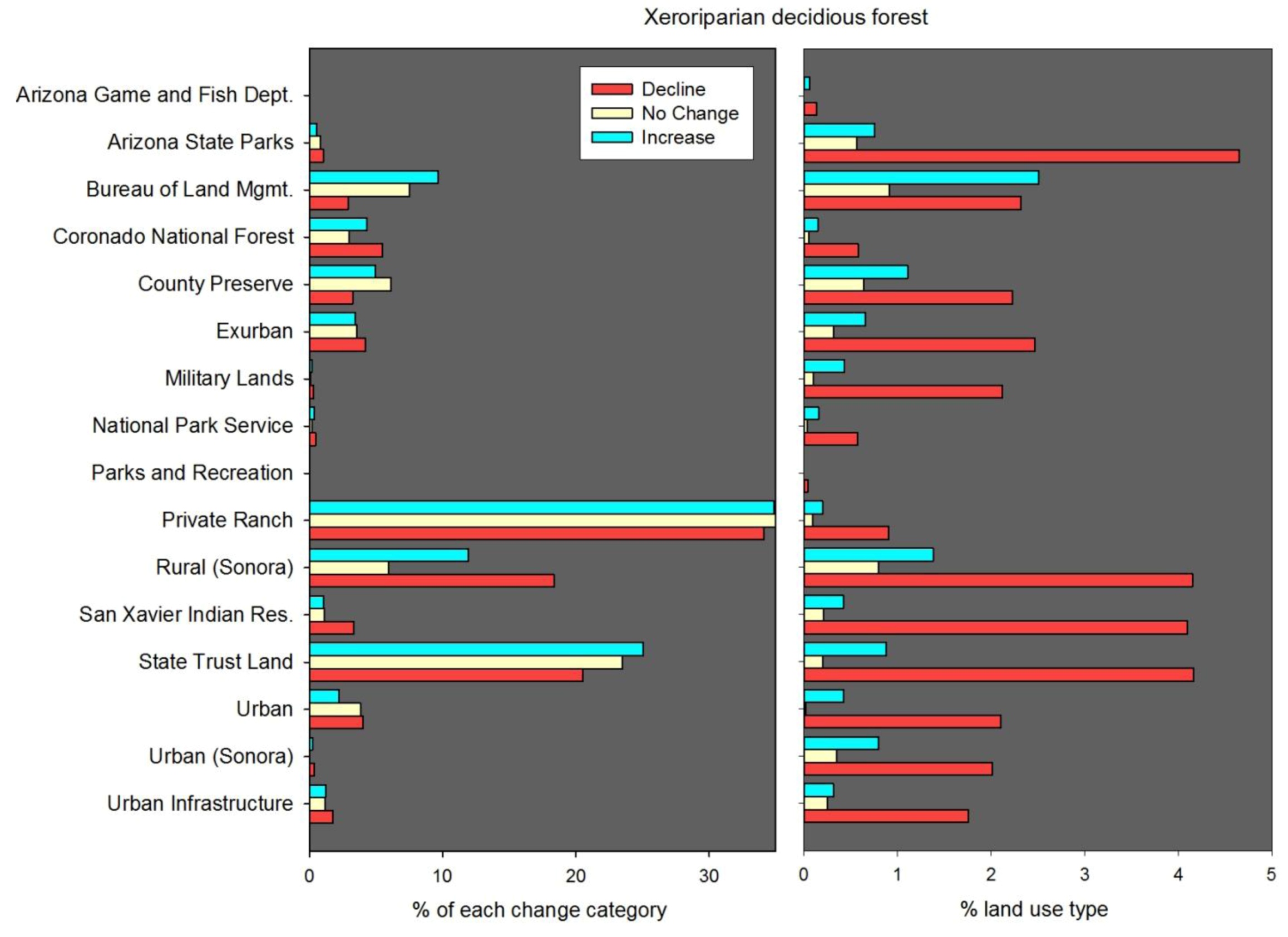
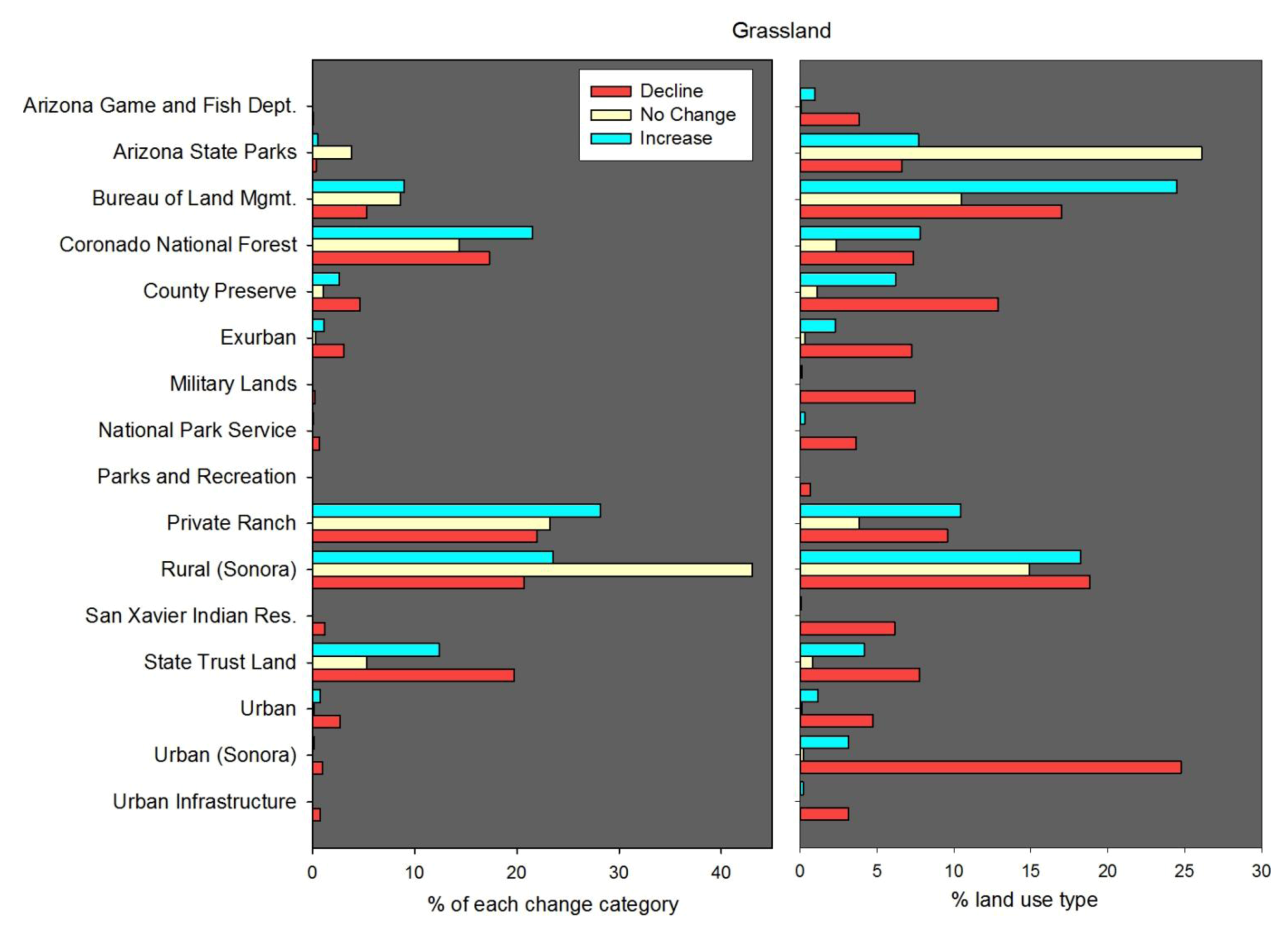
2.3. Broad Changes within Different Land-Use Units


2.4. Change within Ecoregions, 1979–2009

| Vegetation | Total Change within Each Ecoregion (%) | Ecoregion Specific | ||
|---|---|---|---|---|
| % Decline | % No Change | % Increase | ||
| Sonoran deciduous forest | 42.2 | 70.9 | 11.1 | 18.0 |
| Madrean deciduous forest | 57.8 | 67.6 | 10.1 | 22.4 |
| Sonoran grassland | 12.2 | 84.2 | 1.5 | 14.3 |
| Madrean grassland | 87.8 | 39.0 | 19.3 | 41.7 |
| Land Use/Land Ownership | Madrean Grassland (ha) | Sonoran Grassland (ha) | ||||
|---|---|---|---|---|---|---|
| Decline | No Change | Increase | Decline | No Change | Increase | |
| Arizona Game and Fish Dept. | 55 | 1 | 14 | NA | NA | NA |
| Arizona State Parks | 240 | 951 | 281 | 1 | 0 | 0 |
| Bureau of Land Mgmt. | 3447 | 2138 | 4985 | 13 | 0 | 1 |
| Coronado National Forest | 9976 | 3557 | 11709 | 196 | 0 | 1 |
| County Preserve | 2426 | 263 | 1361 | 612 | 0 | 106 |
| Exurban | 1250 | 80 | 580 | 746 | 2 | 51 |
| National Park Service | 159 | 0 | 37 | 335 | 0 | 1 |
| Parks and Recreation | NA | NA | NA | 17 | 0 | 1 |
| Private Ranch | 11531 | 5693 | 14963 | 2773 | 65 | 648 |
| Rural (Sonora) | 13473 | 10663 | 13032 | NA | NA | NA |
| San Xavier Indian Res. | NA | NA | NA | 805 | 1 | 12 |
| State Trust Land | 5455 | 1170 | 5513 | 7842 | 198 | 1647 |
| Urban | 919 | 35 | 404 | 848 | 1 | 22 |
| Urban (Sonora) | 661 | 6 | 84 | NA | NA | NA |
| Urban Infrastructure | NA | NA | NA | 497 | 1 | 30 |
2.5. Photographic Evidence of Change during the Land-Cover Period


2.6. Discussion
3. Conclusions
Acknowledgments
Conflict of Interest
References
- Turner, B.L.; Lambin, E.F.; Reenberg, A. The emergence of land change science for global environmental change and sustainability. Proc. Natl. Acad. Sci. USA 2007, 104, 20666–20671. [Google Scholar] [CrossRef]
- Stafford Smith, D.M.; McKeon, G.M.; Watson, I.W.; Henry, B.K.; Stone, G.S.; Hall, W.B.; Howden, S.M. Learning from episodes of degradation and recovery in variable Australian rangelands. Proc. Natl. Acad. Sci. USA 2007, 104, 20690–20695. [Google Scholar] [Green Version]
- Reynolds, J.F.; Smith, D.M.S.; Lambin, E.F.; Turner, B.L.; Mortimore, M.; Batterbury, S.P.J.; Downing, T.E.; Dowlatabadi, H.; Fernández, R.J.; Herrick, J.E.; et al. Global desertification: Building a science for dryland development. Science 2007, 316, 847–851. [Google Scholar]
- Bahre, C.J.; Bradbury, D.E. Vegetation change along the arizona-sonora boundary. An. Assoc. Am. Geogr. 1978, 68, 145–165. [Google Scholar] [CrossRef]
- Bahre, C.J. A Legacy of Change: Historic Human Impact on Vegetation in the Arizona Borderlands; University of Arizona Press: Tucson, AZ, USA, 1991. [Google Scholar]
- Swetnam, T.W.; Allen, C.D.; Betancourt, J.L. Applied historical ecology: Using the past to manage for the future. Ecol. Appl. 1999, 9, 1189–1206. [Google Scholar] [CrossRef]
- Turner, R.M.; Webb, R.H.; Bowers, J.E.; Hastings, J.R. The Changing Mile Revisited: An Ecological Study of Vegetation Change with Time in the Lower Mile of an Arid and Semiarid Region; University of Arizona Press: Tucson, AZ, USA, 2003. [Google Scholar]
- Bahre, C.J.; Shelton, M.L. Historic vegetation change, mesquite increases, and climate in southeastern Arizona. J. Biogeogr. 1993, 20, 489–504. [Google Scholar] [CrossRef]
- Archer, S. Tree-grass dynamics in a Prosopis-thornscrub savanna parkland: Reconstructing the past and predicting the future. Ecoscience 1995, 2, 83–99. [Google Scholar]
- Webb, R.H.; Leake, S.A.; Turner, R.M. The Ribbon of Green: Change in Riparian Vegetation in the Southwestern United States; University of Arizona Press: Tucson, AZ, USA, 2007. [Google Scholar]
- Poff, B.; Koestner, K.A.; Neary, D.G.; Henderson, V. Threats to riparian ecosystems in Western North America: An analysis of existing literature1. J. Am. Water Resour. Assoc. 2011, 47, 1241–1254. [Google Scholar] [CrossRef]
- Wilcox, B.P.; Thurow, T.L. Emerging issues in rangeland ecohydrology: Vegetation change and the water cycle. Rangel. Ecol. Manag. 2006, 59, 220–224. [Google Scholar] [CrossRef]
- Polyakov, V.O.; Nearing, M.A.; Stone, J.J.; Hamerlynck, E.P.; Nichols, M.H.; Holifield Collins, C.D.; Scott, R.L. Runoff and erosional responses to a drought-induced shift in a desert grassland community composition. J. Geophys. Res. 2010, 115, G04027. [Google Scholar] [CrossRef]
- Wilcox, B.P.; Turnbull, L.; Young, M.H.; Williams, C.J.; Ravi, S.; Seyfried, M.S.; Bowling, D.R.; Scott, R.L.; Germino, M.J.; Caldwell, T.G.; et al. Invasion of shrublands by exotic grasses: Ecohydrological consequences in cold versus warm deserts. Ecohydrology 2011, 5, 160–173. [Google Scholar]
- McClaran, M.P.; van Devender, T.R. The Desert Grassland; The University of Arizona Press: Tucson, AZ, USA, 1995. [Google Scholar]
- McPherson, G.R. Ecology and Management of North American Savannas; The University of Arizona Press: Tucson, AZ, USA, 1997. [Google Scholar]
- Wilson, T.B.; Thompson, T.L. Soil nutrient distributions of mesquite-dominated desert grasslands: Changes in time and space. Geoderma 2005, 126, 301–315. [Google Scholar] [CrossRef]
- Havstad, K.M.; James, D. Prescribed burning to affect a state transition in a shrub-encroached desert grassland. J. Arid Environ. 2010, 74, 1324–1328. [Google Scholar] [CrossRef]
- Brown, J.R.; Archer, S. Woody plant seed dispersal and gap formation in a North American subtropical savanna woodland: The role of domestic herbivores. Vegetatio 1988, 73, 73–80. [Google Scholar] [CrossRef]
- Brown, J.H.; Valone, T.J.; Curtin, C.G. Reorganization of an arid ecosystem in response to recent climate change. Proc. Natl. Acad. Sci. USA 1997, 94, 9729–9733. [Google Scholar] [CrossRef]
- Naiman, R.J.; Decamps, H.; McClain, M.E. Riparia: Ecology, Conservation, and Management of Streamside Communities; Elsevier Acadmeic Press: San Diego, CA, USA, 2005. [Google Scholar]
- Norman, L.M.; Villarreal, M.L.; Lara-Valencia, F.; Yuan, Y.; Nie, W.; Wilson, S.; Amaya, G.; Sleeter, R. Mapping socio-environmentally vulnerable populations access and exposure to ecosystem services at the US-Mexico borderlands. Appl. Geogr. 2012, 34, 413–424. [Google Scholar] [CrossRef]
- Poff, N.L.; Allan, J.D.; Bain, M.B.; Karr, J.R.; Prestegaard, K.L.; Richter, B.D.; Sparks, R.E.; Stromberg, J.C. The natural flow regime. BioScience 1997, 47, 769–784. [Google Scholar] [CrossRef]
- Belsky, A.J.; Matzke, A.; Uselman, S. Survey of livestock influences on stream and riparian ecosystems in the western United States. J. Soil Water Conserv. 1999, 54, 419–431. [Google Scholar]
- Sheridan, T.E. Cows, condos, and the contested commons: The political ecology of ranching on the Arizona-Sonora Borderlands. Hum. Organ. 2001, 60, 141–152. [Google Scholar]
- Curtin, C.G.; Sayre, N.F.; Lane, B.D. Transformations of the Chihuahuan Borderlands: Grazing, fragmentation, and biodiversity conservation in desert grasslands. Environ. Sci. Policy 2002, 5, 55–68. [Google Scholar] [CrossRef]
- Sayre, N.; deBuys, W.; Bestelmeyer, B.; Havstad, K. “The Range Problem” after a century of rangeland science: New research themes for altered landscapes. Rangel. Ecol. Manag. 2012. [Google Scholar] [CrossRef]
- Martin, S.C.; Severson, K.E. Vegetation response to the Santa Rita grazing system. J. Range Manag. 1988, 41, 291–295. [Google Scholar] [CrossRef]
- Geiger, E.L.; McPherson, G.R. Response of semi-desert grasslands invaded by non-native grasses to altered disturbance regimes. J. Biogeogr. 2005, 32, 895–902. [Google Scholar] [CrossRef]
- Briske, D.D.; Derner, J.D.; Brown, J.R.; Fuhlendorf, S.D.; Teague, W.R.; Havstad, K.M.; Gillen, R.L.; Ash, A.J.; Willms, W.D. Rotational grazing on rangelands: Reconciliation of perception and experimental evidence. Rangel. Ecol. Manag. 2008, 61, 3–17. [Google Scholar] [CrossRef]
- Peters, D.P.C.; Bestelmeyer, B.T.; Herrick, J.E.; Fredrickson, E.L.; Monger, H.C.; Havstad, K.M. Disentangling complex landscapes: New insights into arid and semiarid system dynamics. BioScience 2006, 56, 491–501. [Google Scholar] [CrossRef]
- Bestelmeyer, B.T.; Goolsby, D.P.; Archer, S.R. Spatial perspectives in state-and-transition models: A missing link to land management? J. Appl. Ecol. 2011, 48, 746–757. [Google Scholar] [CrossRef]
- Okin, G.S.; Parsons, A.J.; Wainwright, J.; Herrick, J.E.; Bestelmeyer, B.T.; Peters, D.C.; Fredrickson, E.L. Do changes in connectivity explain desertification? BioScience 2009, 59, 237–244. [Google Scholar] [CrossRef]
- Hart, R.H.; Laycock, W.A. Repeat photography on range and forest lands in the western United States. J. Range Manag. 1996, 49, 60–67. [Google Scholar] [CrossRef]
- Webb, R.H.; Boyer, D.E.; Turner, R.M. Repeat Photography: Methods and Applications in the Natural Sciences; Island Press: Washington, DC, USA, 2010. [Google Scholar]
- Vankat, J.L.; Major, J. Vegetation changes in sequoia national park, California. J. Biogeogr. 1978, 5, 377–402. [Google Scholar] [CrossRef]
- Webb, R.H.; Steiger, J.W.; Newman, E.B. The Effects of Disturbance on Desert Vegetation in Death Valley National Monument, California; US Geological Survey Bulletin 1793; US Government Printing Office: Washington, DC, USA, 1988; p. 103. [Google Scholar]
- Bowers, J.E.; Webb, R.H.; Rondeau, R.J. Longevity, recruitment and mortality of desert plants in Grand Canyon, Arizona, USA. J. Veg. Sci. 1995, 6, 551–564. [Google Scholar] [CrossRef]
- Clay, G.R.; Marsh, S.E. Monitoring forest transitions using scanned ground photographs as a primary data source. Photogramm. Eng. Remote Sensing 2001, 67, 319–330. [Google Scholar]
- Manier, D.J.; Laven, R.D. Changes in landscape patterns associated with the persistence of aspen (Populus tremuloides Michx.) on the western slope of the Rocky Mountains, Colorado. For. Ecol. Manag. 2002, 167, 263–284. [Google Scholar] [CrossRef]
- Hoffman, T.M.; Todd, S.W. Using Fixed Point Photography, Field Surveys, and GIS to Monitor Environmental Change: An Example from Riemvasmaak, South Africa. In Repeat Photography: Methods and Applications in the Natural Sciences; University of Arizona Press: Tucson, AZ, USA, 2010; pp. 46–56. [Google Scholar]
- McClaran, M.P.; Browning, D.M.; Huang, C.-Y. Temporal Dynamics and Spatial Variability in Desert Grassland Vegetation. In Repeat Photography: Methods and Applications in the Natural Sciences; University of Arizona Press: Tucson, AZ, USA, 2010; pp. 145–166. [Google Scholar]
- Clark, P.E.; Hardegree, S.P. Quantifying vegetation change by point sampling landscape photography time series. Rangel. Ecol. Manag. 2005, 58, 588–597. [Google Scholar] [CrossRef]
- Tape, K.; Sturm, M.; Racine, C. The evidence for shrub expansion in Northern Alaska and the Pan-Arctic. Glob. Chang. Biol. 2006, 12, 686–702. [Google Scholar] [CrossRef]
- Bullock, S.H.; Turner, R.M. Plant Population Fluxes in the Sonoran Desert shown by Repeat Photography. In Repeat Photography: Methods and Applications in the Natural Sciences; University of Arizona Press: Tucson, AZ, USA, 2010; pp. 119–132. [Google Scholar]
- Kull, C.A. Historical landscape repeat photography as a tool for land use change research. Nor. Geogr. Tidsskr. Nor. J. Geogr. 2005, 59, 253–268. [Google Scholar] [CrossRef]
- De Mûelenaere, S.; Frankl, A.; Haile, M.; Poesen, J.; Deckers, J.; Munro, N.; Veraverbeke, S.; Nyssen, J. Historical landscape photographs for calibration of Landsat land use/cover in the northern Ethiopian Highlands. Land Degrad. Develop. 2012. [Google Scholar] [CrossRef] [Green Version]
- Omernik, J.M. Ecoregions of the conterminous United States. An. Assoc. Am. Geogr. 1987, 77, 118–125. [Google Scholar] [CrossRef]
- Villarreal, M.L.; Norman, L.M.; Wallace, C.; van Riper, C., III. A Multitemporal (1979–2009) Land-use/Land-cover Dataset of the Binational Santa Cruz Watershed; US Geological Survey Open-File Report 2011-1131; US Government Printing Office: Washington, DC, USA, 2011; p. 26. [Google Scholar]
- Homer, C.; Huang, C.; Yang, L.; Wylie, B.; Coan, M. Development of a 2001 national landcover database for the United States. Photogramm. Eng. Remote Sensing 2004, 70, 829–840. [Google Scholar]
- Chavez, P.S. Image-based atmospheric corrections—Revisited and improved. Photogramm. Eng. Remote Sensing 1996, 62, 1025–1036. [Google Scholar]
- Collins, J.B.; Woodcock, C.E. An assessment of several linear change detection techniques for mapping forest mortality using multitemporal Landsat TM data. Remote Sens. Environ. 1996, 56, 66–77. [Google Scholar] [CrossRef]
- Lawrence, R.L.; Wright, A. Rule-based classification systems using classification and regression tree (CART) analysis. Photogramm. Eng. Remote Sensing 2001, 67, 1137–1142. [Google Scholar]
- Mas, J.-F. Monitoring land-cover changes: A comparison of change detection techniques. Int. J. Remote Sens. 1999, 20, 139–152. [Google Scholar] [CrossRef]
- Coppin, P.; Jonckheere, I.; Nackaerts, K.; Muys, B.; Lambin, E. Digital change detection methods in ecosystem monitoring: A review. Int. J. Remote Sens. 2004, 25, 1565–1596. [Google Scholar] [CrossRef]
- Lu, D.S.; Mausel, P.; Brondizio, E.; Moran, E. Relationships between forest stand parameters and Landsat TM spectral responses in the Brazilian Amazon Basin. For. Ecol. Manag. 2004, 198, 149–167. [Google Scholar] [CrossRef]
- Gillanders, S.N.; Coops, N.C.; Wulder, M.A.; Gergel, S.E.; Nelson, T. Multitemporal remote sensing of landscape dynamics and pattern change: Describing natural and anthropogenic trends. Prog. Phys. Geogr. 2008, 32, 503–528. [Google Scholar] [CrossRef]
- Webb, R.H.; Boyer, D.E.; Turner, R.M. The Desert Laboratory Repeat Photography Collection—An Invaluable Archive Documenting Landscape Change; US Geological Survey Fact Sheet 2007-3046; US Government Printing Office: Washington, DC, USA, 2007; p. 4. [Google Scholar]
- Zier, J.L.; Baker, W.L. A century of vegetation change in the San Juan Mountains, Colorado: An analysis using repeat photography. For. Ecol. Manag. 2006, 228, 251–262. [Google Scholar] [CrossRef]
- Webb, R.H.; Betancourt, J.L.; Johnson, R.R.; Turner, R.W. Requiem for a River: Historic Change in the Santa Cruz River near Tucson; Univerity of Arizona Press: Tucson, AZ, USA, 2014. [Google Scholar]
- Carter, M.G. Effects of drougth on mesquite. J. Range Manag. 1964, 17, 275–276. [Google Scholar] [CrossRef]
- Seager, R.; Ting, M.; Held, I.; Kushnir, Y.; Lu, J.; Vecchi, G.; Huang, H.-P.; Harnik, N.; Leetmaa, A.; Lau, N.-C.; et al. Model Projections of an Imminent Transition to a More Arid Climate in Southwestern North America. Science 2007, 316, 1181–1184. [Google Scholar] [CrossRef]
- Anable, M.E.; McClaran, M.P.; Ruyle, G.B. Spread of introduced Lehmann lovegrass Eragrostis lehmanniana Nees. in Southern Arizona, USA. Biol. Conserv. 1992, 61, 181–188. [Google Scholar] [CrossRef]
- Williams, D.; Baruch, Z. African Grass Invasion in the Americas: Ecosystem Consequences and the Role of Ecophysiology. Biol. Invas. 2000, 2, 123–140. [Google Scholar] [CrossRef]
- Jones, Z.F.; Bock, C.E. The Botteri’s sparrow and exotic Arizona grasslands: An ecological trap or habitat regained? Condor 2005, 107, 731–741. [Google Scholar]
- National Landscape Conservation System, Las Ciénegas National Conservation Area FY 2011 Managers Annual Report; US Bureau of Land Management: Phoenix, AZ, USA, 2011; p. 26.
- Debano, L.F.; Schmidt, L.J. Potential for enhancing riparian habitats in the southwestern United States with watershed practices. For. Ecol. Manag. 1990, 33–34, 385–403. [Google Scholar] [CrossRef]
- Malcom, J.; Radke, W.R. Effects of riparian and wetland restoration on an avian community in southeast Arizona, USA. Open Conserv. Biol. J. 2008, 2, 30–36. [Google Scholar] [CrossRef]
- Browning, D.M.; Archer, S.R.; Asner, G.P.; McClaran, M.P.; Wessman, C.A. Woody plants in grasslands: Post-encroachment stand dynamics. Ecol. Appl. 2008, 18, 928–944. [Google Scholar] [CrossRef]
- Villarreal, M.L.; Drake, S.; Marsh, S.E.; McCoy, A.L. The influence of wastewater subsidy, flood disturbance and neighbouring land use on current and historical patterns of riparian vegetation in a semi-arid watershed. River Res. Appl. 2012, 28, 1230–1245. [Google Scholar] [CrossRef]
© 2013 by the authors; licensee MDPI, Basel, Switzerland. This article is an open access article distributed under the terms and conditions of the Creative Commons Attribution license (http://creativecommons.org/licenses/by/3.0/).
Share and Cite
Villarreal, M.L.; Norman, L.M.; Webb, R.H.; Turner, R.M. Historical and Contemporary Geographic Data Reveal Complex Spatial and Temporal Responses of Vegetation to Climate and Land Stewardship. Land 2013, 2, 194-224. https://doi.org/10.3390/land2020194
Villarreal ML, Norman LM, Webb RH, Turner RM. Historical and Contemporary Geographic Data Reveal Complex Spatial and Temporal Responses of Vegetation to Climate and Land Stewardship. Land. 2013; 2(2):194-224. https://doi.org/10.3390/land2020194
Chicago/Turabian StyleVillarreal, Miguel L., Laura M. Norman, Robert H. Webb, and Raymond M. Turner. 2013. "Historical and Contemporary Geographic Data Reveal Complex Spatial and Temporal Responses of Vegetation to Climate and Land Stewardship" Land 2, no. 2: 194-224. https://doi.org/10.3390/land2020194
APA StyleVillarreal, M. L., Norman, L. M., Webb, R. H., & Turner, R. M. (2013). Historical and Contemporary Geographic Data Reveal Complex Spatial and Temporal Responses of Vegetation to Climate and Land Stewardship. Land, 2(2), 194-224. https://doi.org/10.3390/land2020194