


Abstract
Rapid urban expansion in tropical coastal cities has intensified vegetation moisture stress, compromising urban resilience and ecological stability. This study investigates the spatial drivers of the Moisture Stress Index (MSI) in Makassar City, Indonesia, by integrating biophysical indicators and land-use characteristics through multi-scale regression analyses. Utilizing dry-season satellite composites (May–August 2025), the research derived Normalized Difference Vegetation Index (NDVI), Land Surface Temperature (LST), and Normalized Difference Built-up Index (NDBI). MSI was modeled using Ordinary Least Squares (OLS) and Geographically Weighted Regression (GWR) across 240 m, 480 m, and 960 m grids. Results indicate that MSI is highly sensitive to urban morphology and land-use configuration. High moisture stress was concentrated in commercial–industrial and dense residential zones characterized by extreme population densities exceeding 28,000 people/km2 and elevated NDBI. In contrast, agricultural zones and open/green spaces provided significant cooling and moisture retention. Comparative performance analysis reveals that the local GWR model significantly outperformed the global OLS model, achieving a substantial reduction in AICc (−10,475.81) and resolving significant spatial autocorrelation to achieve random residuals (z-score = 1.55). The study further confirms that NDBI is the most robust biophysical predictor of MSI. Spatial heterogeneity analysis demonstrated that land-use influences are geographically contingent, with institutional areas showing varied effects based on campus design and canopy presence. These findings emphasize the necessity of scale-aware, climate-adaptive urban planning and demonstrate that GWR provides a high-fidelity tool for identifying neighborhood-level “micro-hotspots” overlooked by global modeling frameworks.
1. Introduction
Vegetation plays a crucial role in regulating tropical land–climate interactions, particularly through its influence on evapotranspiration, surface conductance, and energy exchange processes [1]. Alterations in land cover, especially the conversion of natural vegetation into dense urban areas, can modify surface temperature, intensify climate extremes, and disrupt local hydrological cycles [2]. The Moisture Stress Index (MSI), derived from short-wave infrared and near-infrared reflectance, offers an effective means of detecting vegetation water stress, where higher MSI values indicate reduced canopy moisture and increased physiological stress [3,4]. Mapping MSI has therefore become essential for assessing vegetation health and ecological resilience in rapidly transforming urban environments [5].
Urbanization exacerbates vegetation stress through heat-island intensification, impervious-surface expansion, reduced evapotranspiration, and land-use conversion [6,7]. These processes alter biophysical conditions and generate spatially uneven patterns in urban vegetation condition, particularly where built-up intensity increases across residential, industrial, and transportation land uses [8]. A consistent gradient is often observed between urban cores and peripheral zones: densely built-up centers exhibit higher MSI due to limited vegetation and elevated land-surface temperatures, while suburban and green-belt areas show lower MSI associated with greater vegetation cover [9,10,11].
To better characterize these dynamics, remote-sensing indicators such as the Normalized Difference Vegetation Index (NDVI), built-up land indices (e.g., NDBI/NDBSI), and Land Surface Temperature (LST) are widely applied to quantify vegetation condition, urbanization intensity, and surface thermal characteristics [4,12,13]. Land-use structure, including agricultural land, commercial–industrial areas, institutional zones, open/green spaces, and residential settlements, further shapes vegetation moisture conditions through variations in shading, permeability, evapotranspiration, and anthropogenic heat flux [14,15,16]. Integrating both biophysical and land-use variables offers a more comprehensive understanding of urban vegetation stress.
However, traditional regression models such as Ordinary Least Squares (OLS) assume spatial stationarity, implying constant relationships across geographic space, a condition rarely met in heterogeneous urban landscapes [17]. Geographically Weighted Regression (GWR) addresses this issue by estimating local coefficients, enabling the detection of spatial non-stationarity in ecological and biophysical processes [18,19]. While GWR has been widely applied to vegetation, heat, and built-up analyses, few studies have explored multi-scale MSI modelling that incorporates detailed land-use categories in tropical coastal cities.
Makassar, one of eastern Indonesia’s fastest-growing metropolitan areas, provides a relevant case study due to its rapid urban expansion, substantial land-use conversion, and pronounced gradient from dense urban core to peri-urban agricultural and coastal zones [20,21,22]. These characteristics produce heterogeneous moisture conditions that require multi-scale, spatially explicit modelling.
Therefore, this study aims to: (1) model the spatial distribution of vegetation moisture stress (MSI) across multiple spatial scales; (2) evaluate the relative influence of key biophysical indicators and land-use drivers using Ordinary Least Squares (OLS) and Geographically Weighted Regression (GWR); and (3) examine how these relationships vary with spatial resolution in a rapidly urbanizing tropical coastal city. The findings highlight the importance of integrating multi-scale modelling with land-use analysis to support climate-adaptive planning, vegetation protection, and sustainable landscape management in rapidly urbanizing tropical cities.
2. Research Area
2.1. Geographical and Socio-Ecological Setting
Makassar is the capital of South Sulawesi Province and one of Indonesia’s fastest-growing metropolitan centers, serving as the primary economic, logistical, and maritime gateway for Eastern Indonesia [23]. The total administrative land area is 175.77 km2 [24]. The city occupies a strategic coastal position along the Makassar Strait and exhibits rapid spatial expansion driven by commercial trade, industrial growth, and dense urban settlement [22]. The spatial boundaries and base map framework used throughout this study are retrieved from the Makassar Regional Spatial Plan [25]. This coastal boundary includes several active land reclamation zones, represented as unlabeled white surfaces in the following maps (Figure 1). These areas were intentionally excluded from the biophysical modeling and MSI analysis because they are currently in a state of active construction and lack established land-cover characteristics. Over the past two decades, the urban footprint of Makassar has expanded into peri-urban agricultural zones and coastal lowlands, significantly altering land cover patterns and ecological processes [22].
Figure 1.
Study area delineation of Makassar City, Indonesia, showing administrative boundaries, major road hierarchy (highway, primary, secondary, and local networks), and the city’s geographic position within the national context.
Makassar City is characterized by a predominantly flat coastal topography [26]. As shown in Figure 2a, nearly the entire urban footprint resides at elevations between 0 and 10 m above sea level. This lack of significant relief minimizes topographic influence on moisture stress patterns, placing the focus on anthropogenic drivers.
Figure 2.
Geographic context of Makassar City: (a) Topographical relief and elevation; (b) Population density distribution by district.
Rapid urbanization has seen the population increase from 1.2 million in 2010 to over 1.5 million currently [27]. Spatial variation in population density is extreme (Figure 2b); while peripheral districts like Manggala and Biringkanaya maintain lower densities, the historical urban core districts (e.g., Wajo and Makassar) reach extreme densities of over 28,000 people/km2. These high-density zones align closely with the ‘Very High’ moisture stress hotspots identified in the modeling results.
The city’s tropical monsoon climate, high population density, and accelerated conversion of green spaces make it an important case study for analysing vegetation moisture dynamics under urbanisation pressures. This geographic and socio-ecological context underscores the need to assess how built-up intensity, land surface temperature, and land-use heterogeneity influence vegetation moisture stress across spatial scales.
2.2. Selection of Analytical Scales
The selection of analytical scales is a critical factor in understanding the Modifiable Areal Unit Problem (MAUP) and its impact on the relationship between moisture stress and urban temperature. In this study, we selected three nested grid scales: 240 m, 480 m, and 960 m. These scales were not chosen arbitrarily but were empirically validated to reflect the unique environmental and morphological grain of Makassar City.
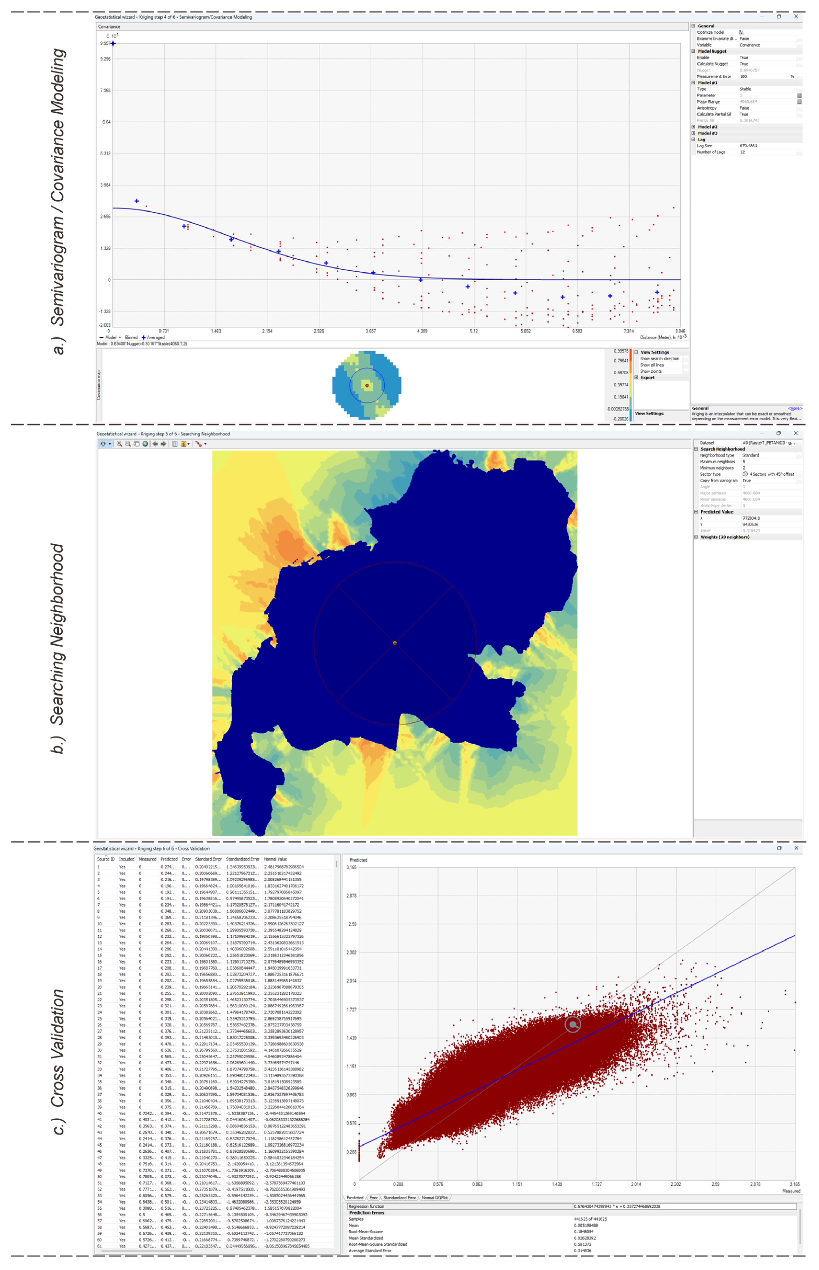
To justify these scales, a geostatistical semivariogram analysis was performed on the source MSI data (see Appendix B Figure A1). The analysis identified a Major Range of 4060.68 m. In geostatistical terms, the “Range” represents the distance at which spatial autocorrelation stabilizes; this result confirms that moisture stress in Makassar is a structured physical phenomenon that remains correlated over a 4 km distance. Consequently, our base 240 m grid, and its subsequent aggregations to 480 m and 960 m, serves as a high-resolution systematic sampling of this broad environmental signal.
Furthermore, the choice of these specific dimensions (240, 480, and 960) follows a nested mathematical alignment (2n hierarchy). Unlike irregular proportions, this nested approach ensures that exactly 16 smaller cells (240 m) fit perfectly into one 960 m cell. This “perfect nesting” is vital for maintaining data integrity during the “zoom out” process, as it eliminates the need for interpolation or resampling at cell boundaries, thereby preventing data loss or statistical “aliasing” that would otherwise invalidate a MAUP analysis.
While traditional urban planning often relies on fixed block sizes, the sprawling and semi-structured growth pattern characteristic of Indonesian cities like Makassar often lacks distinct physical boundaries [28,29]. In this context, a systematic mathematical grid provides a more objective and consistent baseline for detecting environmental patterns. The reliability of this approach is confirmed by the Cross-Validation results (see Appendix B Figure A1), which yielded a Root-Mean-Square error of 0.1848 and a Mean Standardized error of 0.0262. These metrics prove that the model captures the physical reality of Makassar’s moisture stress with high precision and minimal bias, validating the 240 m–960 m hierarchy as a representative framework for the city’s climate analysis.
3. Materials and Methods
This study applied a multi-stage geospatial workflow integrating remote-sensing indices, land-use data, and spatial regression models to assess vegetation moisture stress (MSI) across multiple spatial resolutions in Makassar City, Indonesia. The selection of the three analytical grid resolutions (240 m, 480 m, and 960 m) was designed to capture vegetation moisture dynamics across nested spatial scales relevant to urban environmental analysis and planning. The 240 m grid represents neighborhood-level conditions, allowing detection of fine-scale heterogeneity in land cover, vegetation structure, and microclimate. The 480 m grid corresponds to sub-district or community-scale patterns, balancing spatial detail with analytical stability. The 960 m grid reflects district-level aggregation, enabling assessment of broader urban–rural gradients and large-scale land-use effects.
The methodological framework consisted of four main components: (1) satellite data acquisition and preprocessing, (2) land-use data preparation, (3) computation of MSI and related indices, and (4) statistical modelling using Ordinary Least Squares (OLS) and Geographically Weighted Regression (GWR). All analyses were designed to ensure full reproducibility of the results.
3.1. Satellite Data and Preprocessing
Surface reflectance data from the Sentinel-2 Multi-Spectral Instrument SR Harmonized collection were obtained through the Google Earth Engine (GEE) platform. To capture peak vegetation moisture stress during the dry season, a total of 31 individual image granules (tiles) acquired between May and August 2025 were processed. A complete list of these 31 granules, including their unique System Indices and scene-level Cloud Cover Percentages, is provided in Appendix A Table A1.
While the administrative boundary of Makassar (176.17 km2) is contained within a single Sentinel-2 tile designated T50MQV, every available image asset from the constellation’s 5-day revisit cycle was processed, regardless of scene-level cloud cover. As documented in Appendix A Table A1, the collection includes granules where cloud cover reaches 100%; these were intentionally retained to maximize the temporal depth of the dataset.
To ensure data quality, the Sentinel-2 Scene Classification Layer (SCL) was utilized to perform rigorous pixel-level masking of clouds, cirrus, and shadows. This “pixel harvesting” approach allowed for the extraction of clear-sky observations from all 31 granules, even those with high scene-level interference. By applying a median temporal reducer to the 31-image stack, the final seasonal composite was statistically shielded from outliers and cloud artifacts. As detailed in Appendix A Table A2, this methodology achieved a robust average of 14.04 clear-sky observations per pixel across the study area
The May–August window was strategically selected to minimize atmospheric noise and cloud contamination, which is prevalent in tropical coastal environments during the monsoon season. By targeting the peak dry season, the study “harvests” clear-sky pixels to ensure the highest signal-to-noise ratio for NDVI and LST retrievals.
To validate the study period’s stability, a decadal climatological audit was conducted. Monthly aggregated temperature data (T2m) were retrieved from the ERA5-Land reanalysis [30] and daily precipitation data were sourced from the CHIRPS dataset [31]. Data processing was executed via Google Earth Engine [32], utilizing a custom script to calculate August means for a 10-year baseline (2015–2024) and comparing them against the 2025 study window. As illustrated in Figure 3, the 2025 study window aligns within 0.15 °C of the 10-year annual mean temperature 26.56 °C vs. 26.41 °C. Furthermore, 2025 precipitation levels 87 mm/mo in the study window represent a statistically typical dry season for Makassar, ensuring the findings reflect a stable climate reality rather than a meteorological outlier.
Figure 3.
Makassar Climatological Alignment Data (2015–2025). Data sourced from ECMWF and UCSB, specifically filtered for the Makassar’s official boundaries.
3.2. Land-Use Data Acquisition and Preparation
Official land-use data were obtained from the Makassar Regional Development Agency (BAPPEDA) within its Regional Spatial Plan 2015–2034 Framework (RTRW) in vector (SHP) format [25]. The dataset included five categories: (1) Agriculture (cropland, plantations, rice fields, aquaculture ponds), (2) Commercial–Industrial (markets, retail areas, hotels, workshops, manufacturing zones), (3) Institutional (government buildings, schools, hospitals), (4) Open/Green Space (parks, corridors, urban forests), and (5) Residential (formal and informal settlements). The land-use layer was clipped to the municipal boundary and intersected with analytical grids (240 m, 480 m, and 960 m). For each grid cell, the areal extent (m2), dominant land-use type, and proportional land-use composition (%) were calculated and used as explanatory variables in the regression models.
Land Use and Cover Consistency
To ensure the 2021 BAPPEDA land-use framework remains a valid functional proxy for the 2025 Moisture Stress Index (MSI) analysis, a temporal consistency audit was conducted. Figure 4 presents a comparative Land Cover (LC) analysis between 2021 and 2025. This audit utilizes the ESA WorldCover 10 m dataset [33] to validate the structural stability of the urban fabric. Detailed pixel-level change statistics for all land cover categories are provided in Appendix A (Table A4). The results demonstrate a high degree of structural stability within the urban fabric; the Built-up Area (Class 3) expanded by a marginal 3.29% (42,206 pixels) over the four-year window. While fluctuations were observed in Natural Vegetation (+25.09%), Bare Soil (−25.80%), and Water Bodies (−15.67%), these shifts are primarily attributed to seasonal phenology, varying rainfall patterns, and tidal dynamics during satellite acquisition rather than permanent land-use conversion.
Figure 4.
Comparative Land Cover (LC) Analysis of Makassar City (2021–2025). (a) Land Cover 2025; (b) Land Cover 2021.
Crucially, any environmental variability in these non-built categories is directly accounted for by the integration of real-time 2025 spectral indices (NDVI, NDBI) as independent variables in the GWR models. Consequently, the negligible expansion of the built environment confirms that the 2021 functional zoning remains an accurate spatial framework for the current 2025 biophysical assessment.
3.3. Spectral Index Computation
Four remote-sensing indices were derived to characterize biophysical conditions:
3.3.1. Moisture Stress Index (MSI)
3.3.2. Normalized Difference Vegetation Index (NDVI)
3.3.3. Normalized Difference Built-Up Index (NDBI)
3.3.4. Land Surface Temperature (LST)
Land Surface Temperature (Ts) was retrieved from the Landsat 8 TIRS Band 10 using the Single-Channel (SC) algorithm [36]. This method is suitable for sensors with limited thermal bands or when atmospheric water vapor data is accessible, yielding mean errors typically below 1.5 K. The final values presented in the spatial analysis and maps were converted to degrees Celsius (°C) for better interpretability in an urban planning context. The LST is calculated by inverting the radiative transfer equation as follows:
where
- ϵ is the surface emissivity.
- Lsen is the at-sensor spectral radiance.
- γ and δ are parameters derived from the Planck function, defined by:
In these expressions, Tsen represents the at-sensor brightness temperature, and bγ is a band-specific constant (1324 K for TIRS-1/Band 10). The atmospheric functions (AFs), denoted ψ1, ψ2, and ψ3 are determined from the total atmospheric water vapor content (w) using a second-order polynomial fit:
3.4. Distance from City Center
Urban spatial structure was quantified using two approaches. First, the eight concentric buffers at 2 km intervals centred on Makassar’s central business district to detect distance-related MSI gradients [11]. Second, the Euclidean distance from each grid cell centroid to the city center was calculated and used as a continuous explanatory variable, enabling scale-dependent assessment of distance–MSI relationships [9].
3.5. Statistical Analysis: Ordinary Least Squares (OLS)
Prior to modeling, all variables (MSI, NDVI, NDBI, LST, Distance, and land-use fractions) were rescaled using min–max scaling to a range of [0, 1]. This scale standardization was performed to ensure comparability between coefficients, allowing for the assessment of the relative importance of each predictor across different spatial resolutions. Ordinary Least Squares (OLS) regression was subsequently used to estimate the global relationship between MSI and its predictors:
Model diagnostics included predicted MSI maps, standardized residuals, and adjusted values. OLS was run separately for each grid size (240 m, 480 m, 960 m) to evaluate scale sensitivity [37].
3.6. Geographically Weighted Regression (GWR)
GWR was applied to capture spatially varying relationships:
where denote coordinates and are locally estimated coefficients. In this study, we utilized a Gaussian kernel for the local weight calculations, with a fixed bandwidth set at 140 m [17]. This fixed distance was selected to ensure consistent spatial influence across the study area’s regular grid structure, facilitating the identification of neighborhood-level non-stationarity. For each grid scale (240 m, 480 m, and 960 m), GWR produced local coefficients for all predictors,
- Local maps;
- Predicted MSI surfaces;
- Residual distribution maps.
This enabled identification of spatial non-stationarity and comparison with global OLS results.
3.7. Data Availability and Use of Generative AI
All datasets used in this study (Sentinel-2 image composites, Landsat 8 composites, land-use layers, spatial grids, and regression outputs) are available upon request and will be deposited in a publicly accessible repository prior to publication. Generative AI (ChatGPT-5 Pro) was used solely for language refinement and restructuring of the manuscript text; no AI tools were used for data creation, analysis, or interpretation.
4. Results
4.1. Overview of Spatial Indices
Prior to analyzing the biophysical drivers, the reliability of the seasonal composite was validated through a pixel-level observation audit. Despite the characteristic cloud cover of a tropical coastal environment, the multi-granule integration and high revisit frequency of the Sentinel-2 constellation ensured high data density. The final composite maintained an average of 14.04 clear-sky observations per pixel, with a minimum of 7 and a maximum of 22 valid observations contributing to the median calculation for every location in the study area. This robust temporal depth confirms that the spatial patterns presented in Figure 5 and Figure 6 represent a statistically stable seasonal baseline, free from significant data gaps or cloud-induced artifacts.
Figure 5.
Spatial indices derived from the dry-season composite (May–August 2025): (a) Land Surface Temperature (LST) illustrating urban heat-island intensity; (b) Normalized Difference Vegetation Index (NDVI) showing spatial variation in vegetation density; (c) Normalized Difference Built-up Index (NDBI) mapping impervious-surface distribution; (d) Moisture Stress Index (MSI) indicating spatial patterns of vegetation moisture stress.
Figure 6.
Functional land-use classification of Makassar City. The categories represent an aggregation of official cadastral data into five primary functional zones for modeling purposes.
Figure 5 and Figure 6 illustrate the spatial patterns of key biophysical indices and land-use categories that characterize environmental conditions in Makassar City. These patterns form the empirical basis for evaluating vegetation moisture stress (MSI) across multiple spatial scales.
The Land Surface Temperature (LST) distribution (Figure 5a) reveals a pronounced urban heat-island pattern, with the highest temperatures concentrated within the coastal commercial–industrial belt and dense residential corridors, where impervious surfaces dominate and evaporative cooling is limited. These observations are consistent with evidence that built-up materials intensify heat accumulation and reduce surface moisture in tropical cities [5]. Cooler surface temperatures occur in the northern, eastern, and southern peripheries, where agricultural land and open green spaces are more prevalent, indicating the moderating effects of vegetation and permeable surfaces.
The NDVI distribution (Figure 5b) shows considerable spatial variation in vegetation density. High NDVI values align with agricultural zones, peri-urban vegetation, and designated open spaces, whereas low NDVI values cluster within the central metropolitan core. This inverse spatial relationship between NDVI and LST reflects the well-established role of vegetation in shading and evapotranspiration, which mitigates thermal loading in urban environments [3].
The NDBI map (Figure 5c) further distinguishes built-up areas from vegetated land. High NDBI values coincide with commercial–industrial districts, major road networks, and dense residential blocks, areas that also correspond to high LST and low NDVI. Conversely, agricultural and open-space zones display lower NDBI values, indicating minimal built-up intensity and stronger ecological functioning. These patterns are consistent with findings that impervious expansion alters hydrological processes and contributes to vegetation stress [9].
The MSI distribution (Figure 5d) integrates these biophysical gradients, showing high moisture stress concentrated in dense built-up and commercial–industrial areas, while agricultural land, open green spaces, and vegetated peripheries exhibit lower MSI. This reflects MSI’s sensitivity to thermal conditions and vegetation density, supporting previous work demonstrating its effectiveness in detecting vegetation moisture stress [4].
Figure 6 displays the corresponding land-use configuration of Makassar City. Agricultural zones consistently show low MSI, while commercial–industrial areas align with high LST, high NDBI, and elevated MSI. Institutional areas display mixed conditions depending on vegetation management and building density. Open and green spaces maintain high NDVI and low MSI, functioning as ecological buffers within the city. Residential settlements, especially high-density zones, show moderate to high MSI due to limited vegetation and elevated surface temperatures. These land-use–index associations align with research demonstrating the relationship between landscape composition and microclimatic conditions [15,38].
Together, the spatial patterns reveal a clear urban–rural environmental gradient, reflecting the combined influence of thermal conditions, vegetative cover, built-up intensity, and land-use configuration on moisture stress. These findings establish the empirical foundation for the subsequent OLS and GWR analyses that quantify the contributions of thermal, vegetative, structural, and land-use variables to MSI across multiple spatial scales.
4.2. Vegetation Moisture Stress in Relation to Urban Distance
Figure 7 illustrates the spatial and quantitative relationship between the Moisture Stress Index (MSI) and distance from the city center of Makassar. Using eight concentric buffer rings at 2 km intervals, the average MSI and standard deviation were calculated to evaluate vegetation stress along the urban–rural gradient.
Figure 7.
Spatial and distance-decay patterns of the Moisture Stress Index (MSI) in Makassar City: (a) Concentric 2 km buffer analysis showing the spatial distribution of moisture stress from the city center; (b) Average MSI per 2 km buffer ring illustrating the declining trend of moisture stress with increasing urban distance.
As shown in Figure 7a, higher MSI values (>1.2) are concentrated in the urban core, indicating greater vegetation stress and drier surface conditions. These areas correspond to densely built-up zones with limited vegetation and elevated surface temperatures. In contrast, lower MSI values (<1.0) appear in the outer and peri-urban zones, where vegetation cover and soil moisture are more abundant. This pattern reflects the spatial transition from highly urbanized to greener, cooler areas.
The corresponding graph (Figure 7b) confirms a clear decreasing trend of MSI with distance from the city center. The average MSI declines from approximately 1.3 near the center to 0.95 at 16 km, suggesting that vegetation stress weakens with increasing distance from dense built-up environments. The standard deviation remains relatively stable, indicating consistent spatial variability across zones. This gradient supports the well-established relationship between urbanization intensity and vegetation degradation, where impervious surfaces, heat accumulation, and limited evapotranspiration contribute to higher stress levels [13].
The buffer-based analysis reveals a strong urban–rural gradient of vegetation moisture stress in Makassar. The findings emphasize that urban morphology and surface composition, particularly built-up density and vegetation loss, play a key role in shaping local ecological and climatic conditions.
4.3. Threshold and Percentile Distribution of Indices and Land-Use Proportions Across Multi-Scale Grids
Figure 8 and Figure 9 present the spatial distribution of environmental indices (Distance to City center, LST, NDVI, NDBI, and MSI) and land-use composition (Agriculture, Commercial–Industrial, Institutional, Open Green Space, and Residential) across three analytical grid scales: 240 m, 480 m, and 960 m. This multi-resolution framework enables a systematic evaluation of how grid size influences spatial representation, pattern detection, and the ecological interpretation of urban environmental gradients in Makassar City.
Figure 8.
Spatial distribution of environmental indices across three grid resolutions. Original multi-scale representations illustrating how spatial resolution influences the visibility of urban–environmental gradients for LST, NDVI, NDBI, and MSI at 240 m, 480 m, and 960 m grid scales. These representations highlight micro-, meso-, and macro-scale variability in thermal conditions, vegetation density, and moisture stress.
Figure 9.
Spatial Distribution of Land-Use Proportions Across 240 m, 480 m, and 960 m Grids. Proportional distribution of Agriculture, Commercial–Industrial, Institutional, Open Green Space, and Residential land use across 240 m, 480 m, and 960 m grids in Makassar City.
At the 240 m grid resolution, the maps exhibit high spatial granularity, capturing micro-scale heterogeneity related to urban form and land-cover composition. Distance-to-City Center patterns show well-defined concentric zones radiating from the urban core. The LST and NDBI layers reveal sharply localized hotspots within densely built districts, while NDVI and MSI maps display fine-scale vegetation and moisture variability sensitive to street-level green cover, small parks, and informal vegetation patches. Land-use distributions at this resolution also demonstrate intricate patchiness: agricultural plots, institutional clusters, and commercial–industrial pockets appear highly fragmented, consistent with the complex spatial structure of Makassar’s mixed urban fabric. This level of detail is particularly valuable for neighbourhood-scale diagnostics of vegetation stress, built-up pressure, and micro-climatic variations.
The 480 m grid scale produces a more generalized representation of spatial conditions while retaining the essential urban–environmental gradients. High-temperature zones and built-up intensities in LST and NDBI remain concentrated in the western, central, and coastal districts, but the internal fragmentation seen at 240 m is smoothed into broader continuous areas. NDVI and MSI distributions similarly transition into clearer regional patterns, allowing for more robust detection of medium-scale vegetation and moisture trends. Land-use proportions at this scale better delineate dominant use types, agricultural zones in the north and southeast, commercial corridors along major road networks, and residential concentrations in central districts, making it well suited for sub-district planning applications. The 480 m grid achieves a balance between spatial detail and analytical stability, reducing noise without obscuring meaningful environmental contrasts.
At the 960 m grid resolution, the spatial patterns become substantially aggregated. Thermal and built-up intensities form large contiguous zones, and vegetation and moisture distributions appear more uniform. While this coarser scale is effective in highlighting macro-level environmental gradients, such as the overall west–east and center–periphery contrasts, it inevitably masks the intra-urban heterogeneity apparent in the 240 m and 480 m grids. Land-use proportions at 960 m emphasize district-scale dominance, large residential blocks, major institutional campuses, extensive agricultural belts, but lose micro-parcel variations. This level of spatial aggregation is most appropriate for city-wide analyses and regional environmental policy framing.
Across all resolutions, a consistent set of spatial relationships emerges. High LST and NDBI values cluster in the dense urban core and coastal industrial zones, aligning with low NDVI and high MSI, signifying intense vegetation moisture stress. Conversely, the northern, eastern, and peripheral districts consistently exhibit lower LST, lower NDBI, higher NDVI, and lower MSI, reflecting vegetated and moisture-rich environments. Land-use overlays reinforce these associations: commercial–industrial grids correspond closely with high thermal and moisture stress zones, while open green space and agricultural areas align with cooler and less stressed conditions. Residential areas, particularly high-density settlements, show intermediate patterns influenced by built-form morphology and vegetation availability.
Overall, the comparison of 240 m, 480 m, and 960 m grids underscores the importance of spatial resolution in urban environmental modeling. Fine-resolution grids capture localized environmental stressors and complex land-use mosaics, whereas coarser grids highlight broad structural patterns and city-wide ecological gradients.
4.4. Ordinary Least Squares (OLS) Regression Analysis
The Ordinary Least Squares (OLS) regression models were applied to examine the global relationships between the Moisture Stress Index (MSI) and a set of biophysical and land-use predictors across three spatial resolutions: 240 m, 480 m, and 960 m. The predictor variables included Land Surface Temperature (LST), Normalized Difference Vegetation Index (NDVI), Normalized Difference Built-up Index (NDBI), distance to the city center, and five land-use composition indicators (agriculture, commercial–industrial, institutional, open green space, and residential). Evaluating these models across multiple grid sizes makes it possible to assess how spatial aggregation influences parameter stability and model performance, which is an essential consideration in urban ecological research [37].
Preliminary diagnostic testing confirmed that the model specifications are mathematically stable across all resolutions, with Variance Inflation Factor (VIF) values consistently remaining well below the 5.00 threshold, thereby ensuring that the parameter estimates are not biased by redundant multicollinearity.
4.4.1. Analysis of Explanatory Variables
As presented in Table 1, the standardized coefficients provide a hierarchical ranking of factors contributing to urban moisture deficits. Built-up intensity (NDBI) emerged as the primary and most consistent positive driver of MSI across all spatial scales, indicating that the conversion of natural landscapes into impervious surfaces is the central cause of elevated vegetation stress in Makassar City. This effect is most pronounced at the 240 m neighborhood scale (β = 0.5679, p < 0.0001), where the high density of built structures directly limits the available soil moisture for local flora. Furthermore, the Distance to CBD exhibits a strong positive relationship at the neighborhood scale (β = 0.6875), illustrating a distinct spatial gradient where moisture stress is fundamentally tied to the city’s historical core and radial expansion patterns.
Table 1.
Summary of OLS Results—Model Variable.
Biophysical mitigation is most accurately captured at the 240 m resolution, where NDVI (Vegetation Density) demonstrates a significant negative relationship with MSI (β = −0.0611, p < 0.0001). This inverse correlation confirms that areas with higher biomass density maintain significantly better moisture levels, likely through the combined effects of canopy shading and evapotranspirative cooling. The land-use analysis further elucidates this by showing that Open Space (β = −0.0700) and Agriculture (β = −0.0157) provide critical moisture-retention benefits compared to the general urban matrix. Conversely, commercial–industrial and Institutional zones act as localized stress hotspots, characterized by high pavement ratios that exacerbate the moisture deficit.
The statistical variations observed in Table 1 of the OLS results across the 240 m, 480 m, and 960 m resolutions are a clear manifestation of the Modifiable Areal Unit Problem (MAUP), specifically the scale effect. MAUP occurs when the choice of spatial unit of analysis directly influences the resulting statistical coefficients and significance levels, often hiding or exaggerating relationships as data is aggregated into larger units [39]. In this study, while the Built-up Index (NDBI) remains a robust and consistent driver across all scales (p < 0.0001), biophysical variables such as NDVI and LST lose statistical significance at the intermediate 480 m scale (p = 0.7013 and p = 0.2645, respectively). This loss of significance is attributed to intermediate-scale averaging effects, where the internal heterogeneity of land cover within larger cells smooths out spectral extremes and reduces the variance necessary for the model to identify a consistent relationship. Furthermore, the transition of the Residential land-use coefficient from positive at the 240 m scale to significant negative at the 480 m scale (β = −0.0309) further underscores how the scale of observation modifies the perceived impact of urban drivers on moisture stress intensity.
Addressing MAUP is critical to the validity of this study as it ensures that the test results are not misinterpreted as absolute, but rather as scale-dependent geographic realities. Rather than undermining the reliability of the OLS model, the identification of MAUP enhances the robustness of the findings by revealing the operational scales at which specific environmental drivers’ function. For instance, the persistence of NDBI as a highly significant predictor across all resolutions (p < 0.01) proves that built-up intensity is a dominant, scale-invariant driver of moisture stress, whereas the scale-sensitivity of NDVI suggests that vegetation-based mitigation is a neighborhood-level phenomenon. By explicitly accounting for these variations, the study avoids the “ecological fallacy” of applying broad-scale trends to local-scale interventions, thereby providing more precise and actionable insights for urban ecological management.
4.4.2. Global Model Diagnostics
Table 2 highlights the overall diagnostic performance of the OLS models, which demonstrated exceptional explanatory power with Adjusted R2 values ranging from 0.742 to 0.854. The model performance peaked at the 480 m grid scale (Adj. R2 = 0.8549), identifying this as the optimal resolution for capturing the complex interactions between human-induced land modifications and environmental responses in a dense coastal city. This suggests that while individual buildings drive stress at fine scales, the cumulative impact of land-use planning is most visible at the sub-district level.
Table 2.
OLS Diagnostics.
Despite high predictive accuracy, the Koenker (BP) Statistic was highly significant across all scales (p < 0.0001), formally establishing the presence of spatial non-stationarity. This critical diagnostic proves that the relationships modeled are not spatially consistent; for instance, the mitigating effect of a park in a highly industrialized area may differ significantly from a similar park in a suburban residential zone. This finding provides the definitive statistical justification for transitioning to Geographically Weighted Regression (GWR) to map these localized geographic nuances. Finally, the significant Jarque–Bera statistic confirms that the residuals contain localized biases, likely due to missing spatial predictors, that only a spatially explicit modeling approach can resolve.
4.4.3. Spatial Distribution of Predicted MSI and Residuals
Across all grid resolutions, predicted MSI shows a clear urban–rural gradient that aligns with Makassar’s land-use structure (Figure 10). At the 240 m grid, high MSI values are concentrated in the western and central metropolitan core, where dense commercial–industrial activity, compact residential areas, and high LST produce strong vegetation moisture stress. In contrast, lower MSI values appear in the northern and eastern districts, which contain larger open spaces, urban agriculture, and more continuous vegetation cover.
Figure 10.
Predicted Moisture Stress Index (MSI) and standardized residuals from the Ordinary Least Squares (OLS) model. Across three spatial resolutions (240 m, 480 m, and 960 m), predicted MSI maps illustrate spatial gradients of vegetation moisture stress, whereas residual maps depict patterns of model overprediction and underprediction across Makassar City.
At 480 m, these patterns remain but become more spatially generalized, with high-stress zones forming broader clusters in the west–central area, while low-stress zones persist in vegetated eastern districts. The 960 m grid produces the smoothest spatial surface, highlighting only the major citywide gradient between the densely built western core and the greener eastern periphery.
The standardized residual maps reflect the influence of scale on model performance. At 240 m, localized pockets of over- and under-prediction appear, especially along river corridors, coastal edges, and mixed-land-use zones, indicating fine-scale variability not fully captured by global OLS. Residual clustering decreases substantially at 480 m and is minimal at 960 m, suggesting that coarser grids smooth out local anomalies but may overlook micro-scale environmental processes.
Overall, the predicted MSI and residual distributions confirm a consistent pattern: urban density and imperviousness in the west–central core intensify vegetation moisture stress, while vegetated, open-space, and peri-urban regions in the north and east reduce stress. The reduction in residual variability at coarser grids underscores the scale-dependent nature of MSI modelling.
4.5. Geographically Weighted Regression (GWR) Analysis
The Geographically Weighted Regression (GWR) analysis was conducted to examine spatial non-stationarity in the relationships between MSI and its key predictors: distance to the city center, vegetation density (NDVI), land-surface temperature (LST), built-up intensity (NDBI), and five refined land-use categories (agriculture, commercial–industrial, institutional, open/green space, and residential). Unlike the global OLS model, which assumes uniform relationships across space, GWR produces location-specific coefficients, capturing how the strength and direction of each predictor varies across Makassar’s heterogeneous urban landscape.
The transition from a global Ordinary Least Squares (OLS) framework to a local Geographically Weighted Regression (GWR) at the 240 m scale has significantly enhanced both model parsimony and predictive reliability. As demonstrated by the comparative diagnostics in Table 3, the GWR model, optimized with an adaptive kernel of 140 neighbors, achieved an Adjusted R2 of 0.8465 and a Multiple R2 of 0.8711. This indicates that the local approach effectively captures approximately 85% of the variance in the Moisture Stress Index (MSI), marking a clear improvement over the global model’s Adjusted R2 of 0.8195.
Table 3.
Comparative Performance: Global OLS vs. Local GWR (240 m Grid).
The superiority of the GWR model is further quantified in Table 3 through a dramatic reduction in the Akaike Information Criterion (AICc). The value dropped from 22,086.72 in the OLS model to 11,610.91, a decrease of over 10,475 points that definitively confirms the GWR as a more efficient representation of Makassar’s urban landscape. Furthermore, the model achieved a Sigma (Standard Error) of 5.7228, which reflects higher local precision in predicting moisture stress at the neighborhood scale compared to the global framework.
A critical finding highlighted in the middle section of Table 3 is the highly significant Koenker (BP) statistic of 120.00 (p < 0.0001) produced by the OLS model. This value serves as the primary statistical justification for the study, as it proves that the assumption of spatial uniformity was invalid and that relationships between environmental drivers and MSI vary significantly across the city.
The GWR model effectively addressed this non-stationarity by moving from the rigid uniformity of the OLS to the localized capture of spatial variation. According to the data in Table 3, the GWR model utilized an Effective Number of 289.99 parameters. This expanded flexibility allowed the regression to adapt to local conditions, successfully minimizing Residual Squares to 49,519.75. By allowing the influence of drivers, including NDBI, NDVI, LST, and land-use types like Commercial, Settlement, and Agriculture, to vary geographically, the GWR provides a more robust and actionable framework for targeted urban planning in Makassar.
4.5.1. Spatial Autocorrelation and Scale Diagnostic Validation
The validation of model assumptions through residual analysis reveals a fundamental scale-dependent trend in the spatial reliability of moisture stress predictions. A primary requirement for a robust regression framework is the achievement of independent and randomly distributed residuals, a condition that the global Ordinary Least Squares (OLS) model consistently failed to meet at higher resolutions. As demonstrated by the Global Moran’s I analysis, the OLS model at the 240 m scale exhibited extreme spatial clustering of residuals, yielding a Moran’s Index of 0.5094 and a highly significant z-score of 36.64. This result indicates a less than 1% likelihood that the observed clustered pattern was the result of random chance, proving that the global approach failed to account for the localized geographic drivers of moisture stress.
This pattern of spatial bias persisted as the grid scale was coarsened to 480 m, where the OLS residuals remained significantly clustered with a Moran’s Index of 0.1356 and a z-score of 5.9386. It was only at the 960 m resolution that the global model residuals achieved a statistically random state, characterized by a Moran’s Index of 0.0200 and a non-significant z-score of 0.6847 with a p-value of 0.4935. However, while the 960 m scale satisfies the requirement for spatial independence, it lacks the neighborhood-level granularity essential for actionable urban planning in Makassar. Consequently, the transition to a Geographically Weighted Regression (GWR) at the 240 m scale was required to resolve the identified spatial non-stationarity while preserving high-resolution detail.
The implementation of the GWR model with an optimized adaptive bandwidth of 140 neighbors successfully mitigated the extreme bias identified in the OLS framework. Most critically, the GWR reduced the residual spatial autocorrelation to a Moran’s Index of 0.0215 and a z-score of 1.5535. With a p-value of 0.1202, the residuals at the 240 m scale are no longer significantly different from random, confirming that the local model has successfully satisfied the statistical assumption of spatial independence. These results, which provide the definitive quantitative justification for the local modeling approach, are summarized and compared across scales in Table 4.
Table 4.
Comprehensive Spatial Autocorrelation Comparison.
The visual and statistical confirmation of this transition is presented in Figure 11. The mapping of standardized residuals in Figure 11a demonstrates a predominantly random distribution, with the majority of grid cells falling within the neutral ±1.65 standard deviation range, signifying localized predictive accuracy across the city. This is further verified by the Global Moran’s I report in Figure 11b, where the z-score is clearly situated within the “Random” zone of the distribution curve.
Figure 11.
GWR Residual Diagnostics for 240 m Grid. Panel (a) maps standardized residuals, showing accurate predictions (yellow cells) within the ±1.65 SD range. Panel (b) confirms a Moran’s Index of 0.0215 and a z-score of 1.5535 (p = 0.1202) of the GWR analysis. These results statistically verify a random distribution, satisfying the assumption of spatial independence and resolving the OLS bias.
4.5.2. Comparative Spatial Performance
To evaluate the predictive accuracy of the modeling frameworks, a side-by-side spatial comparison was conducted between the local GWR and global OLS maps at the 240 m resolution, as shown in Figure 10. A Standardized Classification of Predicted MSI was applied to both maps to facilitate a consistent evaluation of moisture stress patterns across Makassar. While the GWR model captured significantly higher local extremes, reaching values in excess of 50, compared to the OLS global average which peaked at approximately 28.8, the ordinal stress levels (ranging from “Very Low” to “Very High”) were synchronized to allow for an objective assessment of localized hotspots.
This standardized comparison reveals that the GWR model (Figure 12b) provides a much higher level of spatial fidelity. It identifies critical moisture-stress “micro-hotspots” in the western and central portions of the city where the compounding effects of high built-up intensity (NDBI) and low vegetation density (NDVI) are most severe. In contrast, the OLS model (Figure 12a) produces a generalized urban–rural gradient that smooths out these localized extremes. For instance, large areas in the central urban core that GWR identifies as “Very High Stress” are generalized by OLS into lower “Moderate” or “Moderately High” categories.
Figure 12.
Standardized Classification of Predicted MSI: (a) Global OLS Model at 240 m resolution; (b) Local GWR Model at 240 m resolution.
The visual disparity between these models is fundamentally emphasized by the spatial autocorrelation metrics summarized in Table 4. While the OLS model at 240 m results in highly clustered residuals (z-score = 36.64), the GWR framework effectively resolves these localized dependencies to achieve a random spatial pattern (z-score = 1.55). This statistical shift confirms that whereas the OLS model suffers from systematic spatial bias, the GWR model successfully captures the non-stationary relationships necessary for reliable neighborhood-level planning.
4.5.3. Spatial Heterogeneity of Biophysical Predictors
While global estimates identify the average strength of environmental drivers, they fail to account for how these relationships shift across the urban landscape. By mapping the local coefficients generated through the GWR framework, this section explores the spatial non-stationarity of biophysical predictors. This localized approach reveals how the influence of urban density, thermal intensity, and biomass on moisture stress is dictated by the specific geographic context of each neighborhood. The spatial distribution of these varying impacts, including distance, LST, NDVI, and NDBI, is visualized in Figure 13.
Figure 13.
Spatial distribution of GWR local coefficients for (a) distance to the city center, (b) land-surface temperature (LST), (c) vegetation density (NDVI), and (d) built-up intensity (NDBI) in Makassar City using the 240 m grid. Higher positive coefficients indicate stronger heating or stress-enhancing effects, while negative coefficients represent cooling or moisture-retention influences.
- Distance to the City Center (Figure 13a)
The GWR distance coefficients display a clear concentric pattern, with strong positive coefficients in the urban core that gradually diminish toward the periphery. This indicates that proximity to the urban center intensifies MSI, likely due to high imperviousness, traffic density, and reduced vegetative cover. Conversely, negative coefficients in rural–peri-urban zones highlight their capacity to retain moisture. This spatial decay pattern aligns with urban–thermal gradients observed in tropical cities [9].
- 2.
- Land Surface Temperature (LST) (Figure 13b)
LST exhibits consistently positive coefficients, but the magnitude varies spatially. The most pronounced thermal influence appears in the western and southern coastal districts, where industrial belts and reclaimed coastal developments trap heat. Cooler eastern and northeastern areas show weaker coefficients, demonstrating vegetation’s moderating influence. These localized thermal effects underscore LST as a spatially dependent driver of vegetation water stress.
- 3.
- Vegetation Density (NDVI) (Figure 13b)
NDVI coefficients are strongly negative across most of the city, reflecting vegetation’s role in reducing MSI through evapotranspiration and canopy moisture conservation. The strongest cooling effects are concentrated in the large urban parks, riparian corridors, and peri-urban agricultural belts, while the weakest influences occur in the dense CBD, where vegetation is sparse.
- 4.
- Built-up Intensity (NDBI) (Figure 13b)
NDBI displays the most spatially coherent pattern among predictors, with positive coefficients dominating the entire urban core. These zones reflect high impervious surface coverage, which amplifies heat storage and reduces moisture infiltration. Lower coefficients in the vegetated periphery indicate weakened built-up effects where natural land cover dominates. NDBI’s spatial consistency reaffirms its status as the most robust predictor of MSI, consistent with earlier OLS results.
4.5.4. Spatial Effects of Land-Use Types
The spatially varying coefficients from the GWR model reveal substantial heterogeneity in how different land-use categories influence Moisture Stress Index (MSI) across Makassar. Unlike global OLS estimates, the GWR outputs highlight locations where specific land uses exert cooling, neutral, or heating contributions to vegetation moisture stress, reflecting the fine-grained mosaic of the city’s urban landscape.
- Agriculture (Figure 14a)Figure 14. Spatial variation in land-use influences on vegetation moisture stress (MSI) based on GWR coefficients. It depicts localized effects of (a) agriculture, (b) commercial–industrial areas, (c) institutional land, (d) open/green space, and (e) residential areas.
Agricultural areas, including cropland, rice fields, and fishpond zones, exert a broadly negative influence on MSI, particularly across the northern and southwestern peripheries, indicating a strong cooling effect linked to moisture-rich surfaces and evapotranspiration. Values in these regions fall within the strong to very strong cooling range (approximately −0.14 to −0.41). In contrast, several mixed-use transition zones near the mid-urban belt display slightly positive coefficients, indicating localized heating effects where agricultural parcels are fragmented or surrounded by dense development. These contrasts underline how agricultural cooling potential diminishes when patches become small, isolated, or encroached by built-up land.
- 2.
- Commercial–Industrial Areas (Figure 14b)
Commercial and industrial land uses show the strongest positive MSI coefficients citywide, indicating pronounced heating effects associated with impervious surfaces, manufacturing zones, logistics areas, and commercial corridors. The most intense heating (>+0.21) is concentrated in coastal industrial belts, the western port-adjacent zone, and commercial corridors extending toward the city center. A weaker positive influence appears in peripheral mixed-commercial clusters. The spatial pattern demonstrates that economic activity nodes significantly amplify vegetation moisture stress due to built-up density, reduced canopy cover, and elevated surface temperatures.
- 3.
- Institutional Areas (Figure 14c)
Institutional land, hospitals, schools, universities, and administrative complexes, presents a mixed pattern, functioning as either cooling or heating depending on their physical landscape context. Large institutional campuses in West and South Makassar exhibit strong negative coefficients (up to −0.14), reflecting extensive shading trees and green open courtyards typical of government and educational facilities. Conversely, institutional parcels embedded in compact neighborhoods or surrounded by arterial traffic corridors show positive MSI values, suggesting slight to moderate heating. This differentiation underscores the variability of institutional design, where vegetation-rich campuses deliver cooling benefits, while high-intensity administrative zones contribute to stress.
- 4.
- Open/Green Space (Figure 14d)
Open and green spaces consistently produce strong cooling effects, with coefficients ranging from −0.69 to −0.18 across extensive portions of West, South, and Northeast Makassar. These areas, urban parks, green corridors, and forest remnants, exert the largest cooling influence among all land-use types. The strongest cooling aligns with continuous green corridors and large parks, whereas fragmented green pockets within dense neighborhoods show weaker but still negative effects. A small number of grids near highly urbanized intersections display neutral or slightly positive effects, indicating that the cooling role of green space is diminished when patches are small or isolated by impervious surroundings.
- 5.
- Residential Areas (Figure 14e)
Residential land use exhibits a highly heterogeneous pattern, reflecting the diversity of housing forms in Makassar. Peripheral suburban and low-density residential areas show modest cooling (down to −0.11), consistent with greater tree cover and lower imperviousness. In contrast, urban core dwellings and informal settlements display strong positive MSI coefficients (+0.25 to +0.5), indicating significant heating effects. These hotspots correspond to dense informal settlement areas with limited vegetation, narrow road networks, and extensive roof-and-wall exposure. The spatial contrast highlights residential morphology as a critical driver of moisture stress: cooling in green, low-density zones and heating in compact, vegetation-poor settlements.
Overall, the land-use GWR results demonstrate that the spatial configuration, density, and ecological structure of land-use parcels shape localized moisture stress dynamics more strongly than land-use type alone. Green infrastructure (open space, agriculture) exhibits spatially persistent cooling effects, whereas commercial–industrial and dense residential areas produce consistent heating effects, with institutional land presenting varied outcomes tied to design and canopy presence.
5. Discussion
The spatial analysis of the Moisture Stress Index (MSI) across Makassar reveals a consistent urban–rural moisture stress gradient, shaped primarily by land surface temperature (LST), vegetation density (NDVI), and built-up intensity (NDBI). The highest MSI values are concentrated in the western and central urban core, characterized by dense development and extensive impervious surfaces, while the eastern and southern peripheries exhibit lower MSI due to greater vegetation cover and heterogeneous land-use mosaics.
5.1. Critical Evaluation of Model Diagnostics and Scale Implications
The multi-scale analysis reveals that spatial resolution and model architecture fundamentally dictate the reliability of moisture stress inferences. Engagement with the model diagnostics indicates that the global OLS framework at the 240 m scale was compromised by extreme spatial autocorrelation, as evidenced by a Moran’s Index of 0.5094 and a z-score of 36.64. In practical terms, this high degree of residual clustering means that the global OLS model failed to account for localized geographic structures, leading to systematic over- or under-predictions in specific urban clusters.
The observed shifts in statistical significance across varying grid sizes provide a clear window into the Modifiable Areal Unit Problem (MAUP). This geographic phenomenon demonstrates that the strength of an environmental relationship is often a byproduct of the chosen spatial container rather than just the physical data itself. Specifically, the scale effect of MAUP is evident as the model transitions from a neighborhood-level (240 m) to a regional (960 m) perspective.
The non-significant results for NDVI and LST at the 480 m resolution represent a specialized case of spatial smoothing. At this specific “intermediate” scale, the grid units become large enough to blend together contrasting land-cover signatures, such as cool, moist garden patches mixed with high-heat pavement, which effectively dilutes the distinct biophysical signals that were clearly visible at finer resolutions. This internal balancing of opposites within the 480 m cells (p = 0.7013 for NDVI) illustrates how data aggregation can inadvertently mask the real-world drivers of vegetation stress.
As the grid scale was coarsened to 960 m, the residuals achieved a random state with a z-score of 0.68 and a p-value of 0.49, suggesting that citywide thermal and land-cover gradients eventually stabilize when local spatial noise is smoothed. However, the diagnostic failure of the OLS at the 240 m and 480 m scales provides the statistical justification for the local modeling approach. By transitioning to a Geographically Weighted Regression (GWR) with 140 neighbors, the spatial non-stationarity that the global model could not handle was resolved.
5.2. Biophysical Dominance and Land-Use Heterogeneity
A notable finding is that biophysical indices, particularly NDBI and NDVI, consistently emerge as stronger predictors of MSI compared to formal land-use categories. This disparity is attributed to intra-category heterogeneity within formal land-use zones. For example, a residential zone in Makassar encompasses both low-density, verdant suburban estates and hyper-dense, informal settlements with minimal canopy cover. This internal variance dilutes the explanatory power of the categorical variable. In contrast, NDBI acts as a more direct, high-fidelity proxy for moisture stress by measuring the spectral signature of impervious surfaces regardless of the plot’s administrative function.
5.3. Spatial Variability of MSI Drivers
The GWR coefficient maps reveal critical spatial nuances that global models obscure, particularly regarding the non-stationary influence of land use. In the peri-urban zones of Tamalanrea and Manggala, agricultural land and undeveloped open spaces act as vital thermal sinks that consistently lower MSI values, yet this cooling influence is highly sensitive to landscape continuity. Where agricultural parcels are fragmented by encroaching residential estates, their ability to mitigate moisture stress is significantly diminished compared to large, contiguous fields. Conversely, the strongest positive associations with MSI are localized in high-intensity economic corridors, particularly in the port-adjacent zones of Tallo and Ujung Tanah. In these environments, the combination of high anthropogenic heat release and near-total absence of tree canopy creates a compounding effect that elevates MSI beyond global predictions. Unlike other variables, the cooling effect of institutional green spaces and parks remains spatially consistent across the city, suggesting that green infrastructure is a universally effective intervention regardless of its location in the urban core or suburban fringe. Furthermore, the GWR successfully distinguishes between residential morphologies, identifying that in high-density districts like Rappocini, residential land use is a significant stress driver due to crowded structures, whereas in lower-density outskirts like Tamalate, similar residential labels are associated with lower MSI values due to better integration with natural land cover.
5.4. Targeted Policy Implications for District-Level Adaptation
The localized findings of the GWR analysis allow for a precision-based planning framework based on the specific biophysical needs of different district groups. As illustrated in Figure 15, the spatial distribution of moisture stress reveals distinct clusters that align with administrative boundaries, providing a clear roadmap for targeted interventions. To facilitate the implementation of these findings, Table 5 synthesizes these spatial results into a concrete policy framework, linking each vulnerability group to specific structural and ecological mandates.
Figure 15.
Predicted Vegetation Moisture Stress Index (MSI) [GWR, 240 Grid] with Administrative Overlay.
Table 5.
District-Specific Policy Framework based on MSI Vulnerability and Characteristics.
Group 1, comprising the urban core districts of Ujung Pandang, Ujung Tanah, Wajo, Bontoala, Makassar, Mariso, Mamajang, and Rappocini, represents the epicenter of moisture stress characterized by hyper-density and high impervious surface fractions. For these districts, intensive structural remediation is required, including mandatory cool-roof albedo requirements and vertical greening for all commercial redevelopments to mitigate the extreme localized stress visible in the map. In the urban core of Wajo and Bontoala, the lack of canopy necessitates these structural interventions, while in Rappocini, the dense building footprints negate traditional residential cooling effects.
The High Vulnerability Group, consisting of Panakkukang, Tallo, and Biringkanaya, presents a mixed MSI signature driven by commercial expansion and massive infrastructure. Biringkanaya provides a unique case where massive housing estates and airport-supporting infrastructure replace natural porous soils, requiring mandates for permeable surfaces and 30% green-cover thresholds for logistics hubs. Finally, the Moderate Vulnerability Group, including Manggala, Tamalate, and Tamalanrea, currently benefits from predominantly very low MSI in their centers and outskirts. Tamalanrea is particularly successful because its center is dominated by institutional campuses and undeveloped areas, proving that contiguous unpaved land is the most effective thermal sink. However, Manggala and Tamalate exhibit an edge effect where sections bordering the dense center are heavily marked with moisture stress in Figure 10, highlighting these areas as critical frontiers where strict protection of green-space continuity is essential to prevent stress overflow.
5.5. Limitations and Future Directions
While this study provides a robust identification of the socio-physical drivers of moisture stress in Makassar, certain extrinsic geographical factors were not explicitly modeled as independent variables. Makassar’s 32 km coastline along the Makassar Strait and the presence of the Jeneberang and Tallo Rivers on its southern and northern border introduce microclimatic complexities, such as the sea breeze effect and riparian thermal regulation. Although our GWR model achieved a high explanatory power (Multiple R2 = 0.8711) and successfully resolved spatial non-stationarity, future research could build upon these findings by incorporating explicit distance-decay indices for water bodies. Furthermore, integrating 3D microclimate simulations or high-frequency sensor networks could help isolate the precise reach of the sea breeze from the structural influences of the built environment. Such research would further refine the thermal management strategies for sprawling coastal cities in the tropics.
6. Conclusions and Recommendations
This study examined vegetation moisture stress (MSI) in Makassar City using OLS and GWR models across three spatial resolutions (240 m, 480 m, and 960 m). By integrating biophysical indicators (NDVI, NDBI, LST), distance to the city center, and detailed land-use categories, the analysis provides a comprehensive understanding of how urban form and land-use structure influence moisture stress in a rapidly growing tropical city. The multi-scale comparison demonstrated that while the 960 m resolution provided the highest statistical stability for global models, the 240 m GWR was essential for capturing neighborhood-level non-stationarity and resolving the significant spatial autocorrelation found in the global OLS residuals.
Among the biophysical predictors, built-up intensity (NDBI) was the strongest and most consistent driver of MSI across all scales, reflecting the dominant role of imperviousness in elevating vegetation stress. Land-use categories further modulated these patterns, with the highest stress levels concentrated in the western commercial–industrial belt and the dense administrative core. While open spaces and agricultural zones in districts like Tamalanrea consistently reduced stress, the GWR results highlighted that this cooling function is highly localized and prone to “stress overflow” at the edges of the central urban districts.
The findings emphasize that climate-responsive urban planning in Makassar must move beyond general greening toward spatially targeted mandates. Priority interventions must be focused on the Very High Vulnerability Group, specifically Wajo, Tallo, Bontoala, and Makassar districts, where hyper-density necessitates structural remediation such as mandatory cool-roof albedo and vertical greening. In the rapidly expanding suburban-industrial zones of Biringkanaya, policies should prioritize green-cover thresholds for logistics hubs and massive estates to mitigate the infrastructure-led stress identified in the GWR results. Finally, the preservation of the “green center” in Tamalanrea and the agricultural buffers in Manggala and Tamalate is a critical priority to prevent the fragmentation of existing thermal sinks. Integrating these district-specific MSI monitoring results into routine planning will support more adaptive, resilient, and evidence-based urban development in Makassar.
Author Contributions
R.P.A.: Conceptualization; Methodology; Investigation; Formal analysis; Data curation; Writing—original draft; Project administration; Resources; Software; Visualization. M.I.: Data curation; Resources; Investigation. A.A.: Methodology; Validation; Writing—review & editing. C.D.: Formal analysis; Software. L.K.: Methodology; Supervision; Funding acquisition; Resources; Validation; Writing—review & editing. All authors have read and agreed to the published version of the manuscript.
Funding
This research received no external funding and the APC was funded by Department of Landscape Planning and Spatial Development, Institute of Landscape Architecture, Urban Planning and Ornamental Horticulture, Hungarian University of Agriculture and Life Sciences (MATE).
Data Availability Statement
The data that support the findings of this study are available upon request from the corresponding author.
Conflicts of Interest
The authors declare no conflict of interests.
Abbreviations
| MSI | Moisture Stress Index |
| OLS | Ordinary Least Squares |
| GWR | Geographically Weighted Regression |
| NDVI | Normalized Difference Vegetation Index |
| LST | Land Surface Temperature |
| NDBI | Normalized Difference Built-up Index |
| GEE | Google Earth Engine |
| OLI | Operational Land Imager |
| TIRS | Thermal Infrared Sensor on Landsat 8 satellite. |
| AICc | Akaike’s Information Criterion |
| BAPPEDA | Makassar Regional Development Agency |
| CBD | Central Business District |
| GIS | Geographic Information System |
| RS | Remote Sensing |
| GPS | Global Positioning System |
| EO | Earth Observation |
| DEM | Digital Elevation Model |
| NDWI | Normalized Difference Water Index |
| EVI | Enhanced Vegetation Index |
| UHI | Urban Heat Island |
| SEM | Structural Equation Modeling |
| MLR | Multiple Linear Regression |
| MAUP | Modifiable Areal Unit Problem |
| ANOVA | Analysis of Variance |
| p-value | Probability Value |
| DF | Degrees of Freedom |
| SD | Standard Deviation |
| SE | Standard Error |
| IQR | Interquartile Range |
| LULC | Land Use/Land Cover |
| UGB | Urban Growth Boundary |
| SCA | Spatially Constrained Aggregation |
| IR | Infrared General Remote Sensing term |
| SWIR | Short-Wave Infrared |
Appendix A
Table A1.
Metadata for Sentinel-2 Multi-Spectral Instrument granules used in the dry-season composite.
Table A2.
Technical Processing Metadata (Google Earth Engine Output).
Table A3.
Integrated Climatological Audit (2015–2025): Comparison of 4-Month Study Window (May–August) vs. 12-Month Annual Mean.
Table A4.
Quantitative Land Cover Shift between 2021 and 2025.
Appendix B
Figure A1.
Geostatistical Validation of Spatial Autocorrelation and Model Accuracy.
References
- Hales, K.; Neelin, J.D.; Zeng, N. Sensitivity of Tropical Land Climate to Leaf Area Index: Role of Surface Conductance versus Albedo. J. Clim. 2004, 17, 1459–1473. [Google Scholar] [CrossRef] [Scilit]
- Tölle, M.H.; Churiulin, E. Sensitivity of Convection-Permitting Regional Climate Simulations to Changes in Land Cover Input Data: Role of Land Surface Characteristics for Temperature and Climate Extremes. Front. Earth Sci. 2021, 9, 722244. [Google Scholar] [CrossRef] [Scilit]
- Konings, A.G.; Piles, M.; Rötzer, K.; Entekhabi, D. Detecting forest response to droughts with global observations. Nat. Sustain. 2021, 4, 777–786. [Google Scholar] [CrossRef] [Scilit]
- Le, T.S.; Harper, R.; Dell, B. Application of remote sensing in detecting and monitoring plant–water stress in forests. Remote Sens. 2023, 15, 3360. [Google Scholar] [CrossRef] [Scilit]
- Rao, P.; Torreggiani, D.; Tassinari, P.; Rötzer, T.; Pauleit, S.; Rahman, M.A. Do urban green spaces cool cities differently across latitudes? Spatial variability and climatic drivers of vegetation-induced cooling. Sustain. Cities Soc. 2025, 130, 106513. [Google Scholar] [CrossRef] [Scilit]
- Cârlan, I. Identifying urban vegetation stress factors based on open-access remote sensing imagery and field observations. Urban For. Urban Green. 2020, 48, 126565. [Google Scholar] [CrossRef] [Scilit]
- Zhao, S.; Peng, C.; Jiang, H.; Tian, D.; Lei, X.; Zhou, X. Land use change in Asia and the ecological consequences. Ecol. Res. 2006, 21, 890–896. [Google Scholar] [CrossRef] [Scilit]
- Huang, B.; Li, Z.; Dong, C.; Zhu, Z.; Zeng, H. The effects of urbanization on vegetation conditions in coastal zone of China. Prog. Phys. Geogr. 2020, 45, 564–579. [Google Scholar] [CrossRef] [Scilit]
- Niu, L.; Zhang, Z.; Peng, Z.; Liang, Y.; Liu, M.; Jiang, Y.; Wei, J.; Tang, R. Identifying Surface Urban Heat Island Drivers and Their Spatial Heterogeneity in China’s 281 Cities. Remote Sens. 2021, 13, 4428. [Google Scholar] [CrossRef] [Scilit]
- Manalo, J.A.; Matsumoto, J.; Takahashi, H.G.; Villafuerte, M.Q.; Olaguera, L.M.P.; Ren, G.; Cinco, T.A. The effect of urbanization on temperature indices in the Philippines. Int. J. Climatol. 2022, 42, 850–867. [Google Scholar] [CrossRef] [Scilit]
- Li, X.; Meng, Q.; Li, W.; Zhang, C.; Jancso, T.; Mavromatis, S. An explorative study on the proximity of buildings to green spaces in urban areas using remotely sensed imagery. Ann. GIS 2014, 20, 1018–1032. [Google Scholar] [CrossRef] [Scilit]
- Cruz, L.M.; Broqueza, M.J.; Mana-ay, M.; Ramos, R. Spatiotemporal Analysis of Land Surface Temperature in The Philippines from 2019 To 2021. In Proceedings of the 2023 Asian Conference on Remote Sensing (ACRS2023), Taipei, Taiwan, 30 October–3 November 2023. [Google Scholar]
- Li, K.; Li, X.; Hu, W.; Xu, J. Spatiotemporal patterns and driving forces of ecological quality in the Yangtze River Economic Belt using GWRR. Sustainability 2026, 18, 256. [Google Scholar] [CrossRef] [Scilit]
- Findell, K.L.; Berg, A.; Gentine, P.; Krasting, J.P.; Lintner, B.R.; Malyshev, S.; Santanello, J.A., Jr.; Shevliakova, E. The impact of anthropogenic land use and land cover change on regional climate extremes. Nat. Commun. 2017, 8, 989. [Google Scholar] [CrossRef] [Scilit]
- Soydan, O. Effects of landscape composition and patterns on land surface temperature: Urban heat island case study for Nigde, Turkey. Urban Clim. 2020, 34, 100688. [Google Scholar] [CrossRef] [Scilit]
- Weng, Q. Thermal infrared remote sensing for urban climate and environmental studies. ISPRS J. Photogramm. Remote Sens. 2009, 64, 335–344. [Google Scholar] [CrossRef] [Scilit]
- Brunsdon, C.; Fotheringham, A.S.; Charlton, M.E. Geographically weighted regression: A method for exploring spatial nonstationarity. Geogr. Anal. 1996, 28, 281–298. [Google Scholar] [CrossRef] [Scilit]
- Chen, G.; Zhou, Y.; Voogt, J.A.; Stokes, E.C. Remote sensing of diverse urban environments: From single-city to multiple-city studies. Remote Sens. Environ. 2024, 305, 114108. [Google Scholar] [CrossRef] [Scilit]
- Neyns, R.; Hermy, M.; Somers, B. Mapping urban vegetation with high-resolution remote sensing data. Remote Sens. 2022, 14, 1031. [Google Scholar] [CrossRef] [Scilit]
- Firman, T. Demographic and spatial patterns of Indonesia’s recent urbanisation. Popul. Space Place 2004, 10, 421–434. [Google Scholar] [CrossRef] [Scilit]
- Hudalah, D.; Firman, T. Beyond property: Industrial estates and post-suburban transformation in Jakarta metropolitan area. Cities 2012, 29, 40–48. [Google Scholar] [CrossRef] [Scilit]
- Amri, E.; Selintung, M.; Manaf, M.; Nasution, M.A. Suburban Development: Spatial and Physical Transformation of Residence as a Determinant of Settlement Densification in Makassar City, Indonesia. Int. J. Sustain. Dev. Plan. 2023, 18, 2779–2789. [Google Scholar] [CrossRef] [Scilit]
- Makassar City Planning and Development Agency. Policy Setting in the Conflict of Coastal Community Empowerment Policy in Makassar City; Atlantis Press: Dordrecht, The Netherlands, 2023. [Google Scholar] [CrossRef] [Scilit]
- Sattar, A.; Rashid, M.; Mat, R.; Puji, L. A preliminary survey of air quality in Makassar city South Sulawesi Indonesia. J. Teknol. (Sci. Eng.) 2012, 57, 123–136. [Google Scholar] [CrossRef] [Scilit]
- Bappeda Kota Makassar. Rencana Tata Ruang dan Wilayah (RTRW) Kota Makassar 2015–2034; Pemerintah Kota Makassar: Makassar, Indonesia, 2021. [Google Scholar]
- Rohadi, P.P.; Qisthina, N.; Aulia, R.; Arifin, H.S.; Kaswanto, R.L. Urban Landscape Management of Makassar City Based on Waterfront City Concept. IOP Conf. Ser. Earth Environ. Sci. 2024, 1384, 012029. [Google Scholar] [CrossRef] [Scilit]
- Tjandraatmadja, G.; Ahmad, A.; Selintung, M.; Kirono, D.; Larson, S.; Salman, D.; Barkey, R.A.; Talebe, A.; Iman, M.N.; Lipkin, F.; et al. Context and Challenges in Urban Water and Wastewater Services for Makassar, South Sulawesi, Indonesia; A Report Prepared for the CSIRO-AusAID Research Alliance; CSIRO-AusAID Research Alliance: Canberra, Australia, 2012. [Google Scholar]
- Soraya, T.; Camila, S.N.; Maulidia, A. Changing Social Structures in Makassar City Due to Rapid Urbanization in South Sulawesi. J. Soc. Civilecial 2025, 3, 20–33. [Google Scholar] [CrossRef] [Scilit]
- Surya, B.; Salim, A.; Hernita, H.; Suriani, S.; Menne, F.; Rasyidi, E.S. Land use change, urban agglomeration, and urban sprawl: A sustainable development perspective of Makassar City, Indonesia. Land 2021, 10, 556. [Google Scholar] [CrossRef] [Scilit]
- Muñoz-Sabater, J.; Dutra, E.; Agustí-Panareda, A.; Albergel, C.; Arduini, G.; Balsamo, G.; Thépaut, J.N. ERA5-Land: A state-of-the-art global reanalysis dataset for land applications. Earth Syst. Sci. Data 2021, 13, 4349–4383. [Google Scholar] [CrossRef] [Scilit]
- Funk, C.; Peterson, P.; Lansigan, M.; Pedreros, D.; Verdin, J.; Shukla, S.; Husak, G.; Rowland, J.; Harrison, L.; Hoell, A.; et al. The climate hazards infrared precipitation with stations—A new environmental record for monitoring extremes. Sci. Data 2015, 2, 150066. [Google Scholar] [CrossRef] [Scilit] [PubMed]
- Gorelick, N.; Hancher, M.; Dixon, M.; Ilyushchenko, S.; Thau, D.; Moore, R. Google Earth Engine: Planetary-scale geospatial analysis for everyone. Remote Sens. Environ. 2017, 202, 18–27. [Google Scholar] [CrossRef] [Scilit]
- Zanaga, D.; Van De Kerchove, R.; Daems, D.; De Keersmaecker, W.; Brockmann, C.; Kirches, G.; Wevers, J.; Cartus, O.; Santoro, M.; Fritz, S.; et al. ESA WorldCover 10 m 2021 v200. 2022. Available online: https://pure.iiasa.ac.at/id/eprint/18478/ (accessed on 20 November 2025).
- Rouse, J.W.; Haas, R.H.; Schell, J.A.; Deering, D.W. Monitoring vegetation systems in the Great Plains with ERTS. In NASA SP-351: Third Earth Resources Technology Satellite Symposium; NASA: Washington, DC, USA, 1974; pp. 309–317. [Google Scholar]
- Zha, Y.; Gao, J.; Ni, S. Use of normalized difference built-up index in automatically mapping urban areas from TM imagery. Int. J. Remote Sens. 2003, 24, 583–594. [Google Scholar] [CrossRef] [Scilit]
- Jiménez-Muñoz, J.C.; Sobrino, J.A.; Skoković, D.; Mattar, C.; Cristóbal, J. Land surface temperature retrieval methods from Landsat-8 thermal infrared sensor data. IEEE Geosci. Remote Sens. Lett. 2014, 11, 1840–1843. [Google Scholar] [CrossRef] [Scilit]
- Fotheringham, A.S.; Charlton, M.E.; Brunsdon, C. Geographically Weighted Regression: The Analysis of Spatially Varying Relationships; Wiley: Hoboken, NJ, USA, 2002. [Google Scholar]
- Son, N.T.; Chen, C.F.; Chen, C.R.; Thanh, B.X.; Vuong, T.H. Assessment of urbanization and urban heat islands in Ho Chi Minh City, Vietnam using Landsat data. Sustain. Cities Soc. 2017, 30, 150–161. [Google Scholar] [CrossRef] [Scilit]
- Comber, A.; Harris, P. The importance of scale and the MAUP for robust ecosystem service evaluations and landscape decisions. Land 2022, 11, 399. [Google Scholar] [CrossRef] [Scilit]
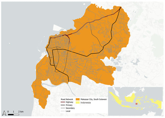
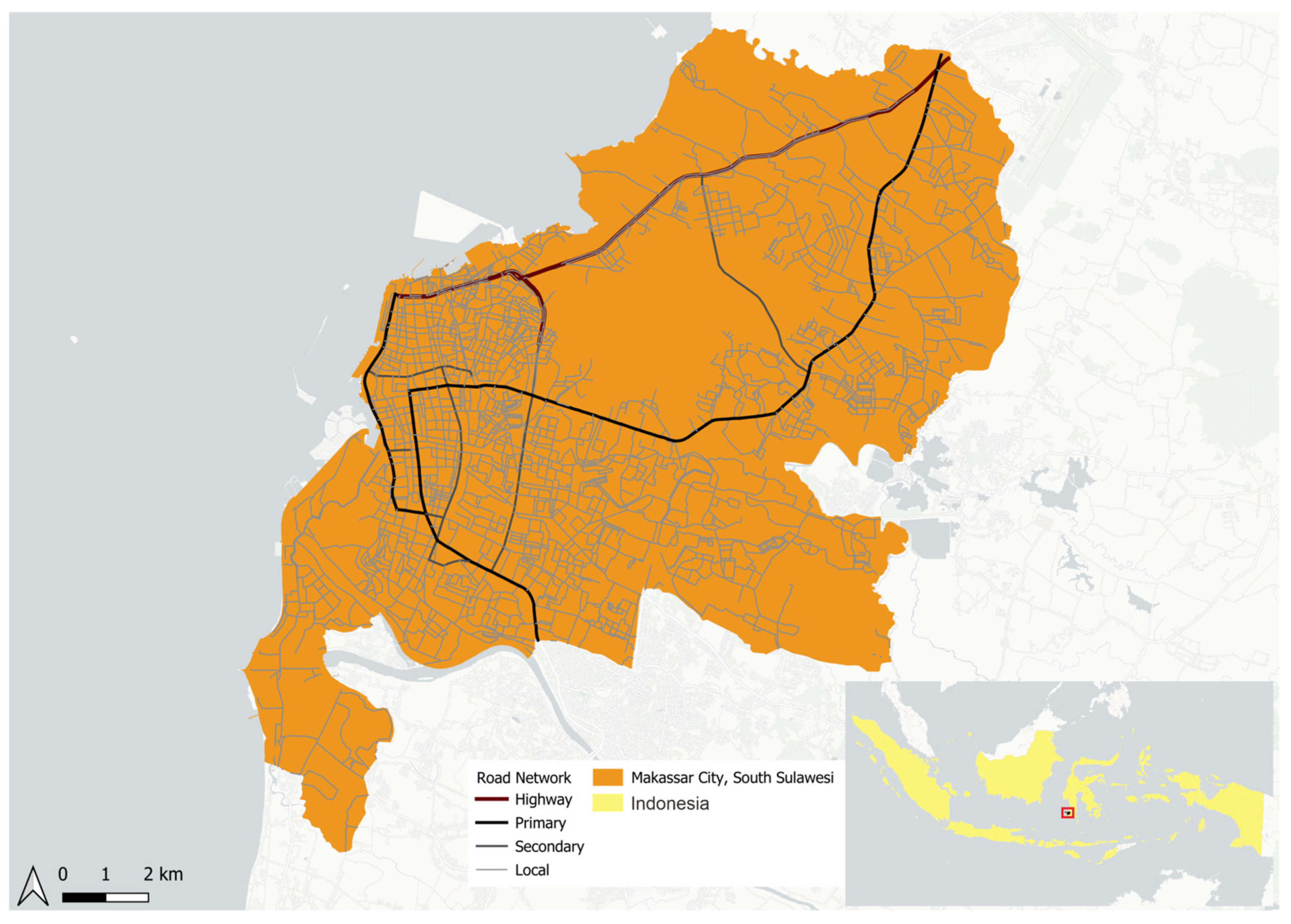
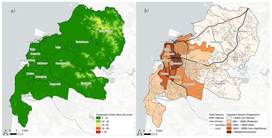
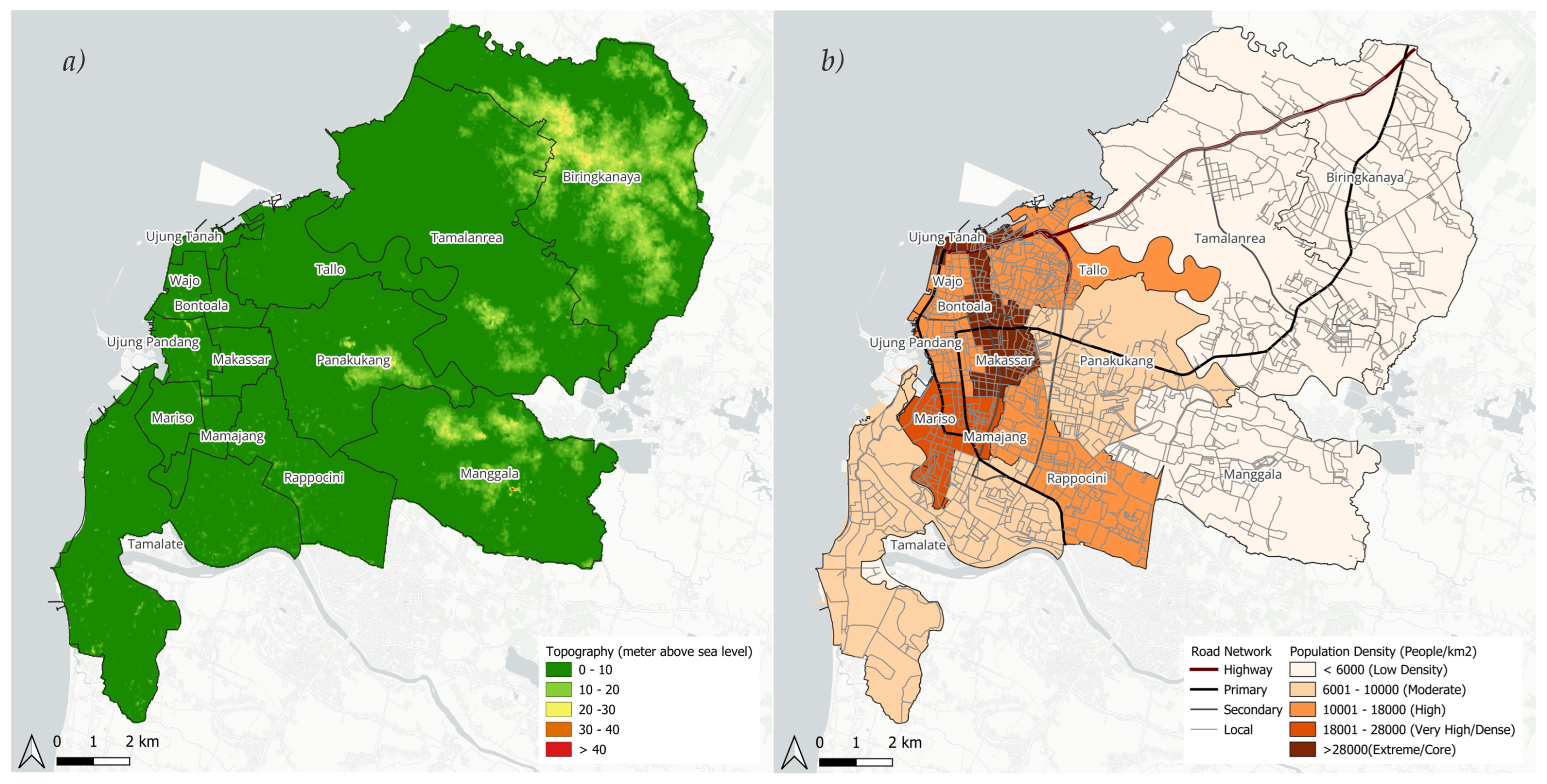
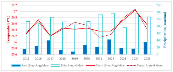
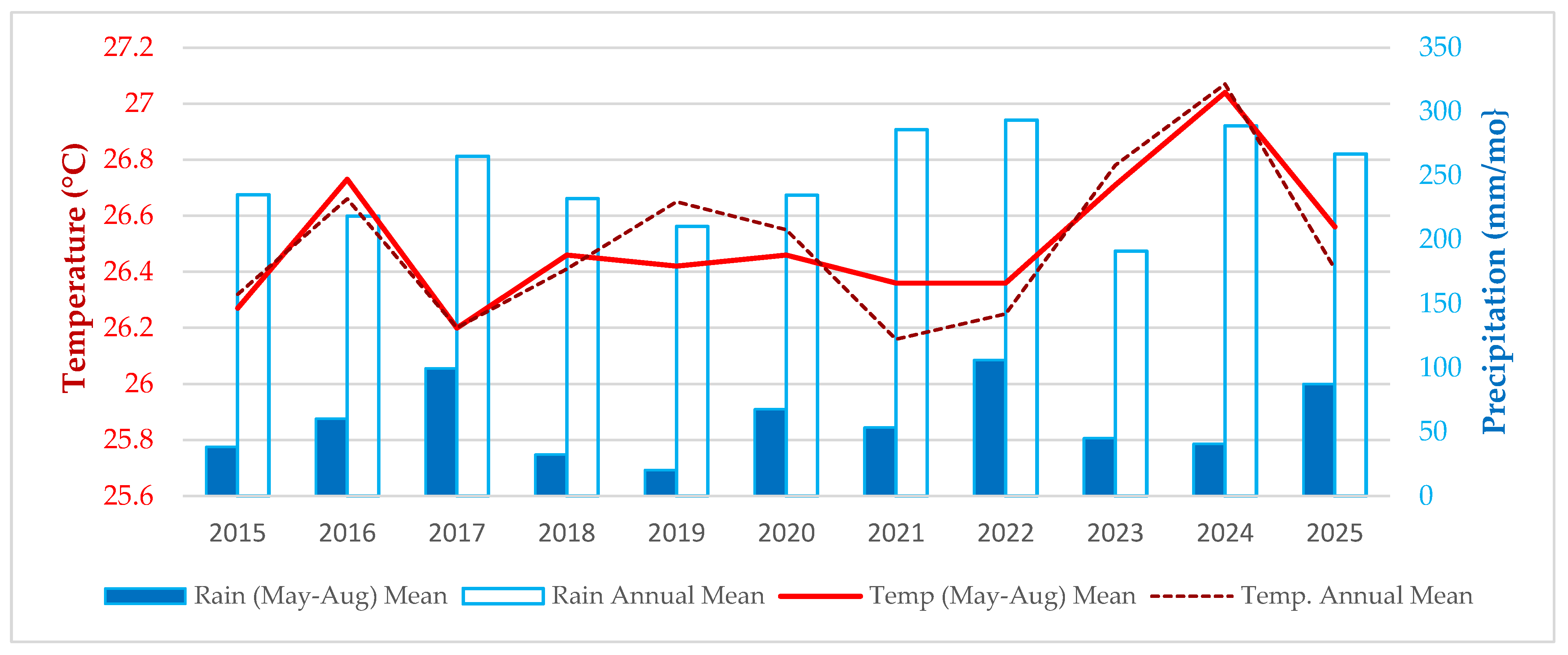
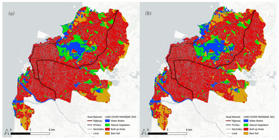
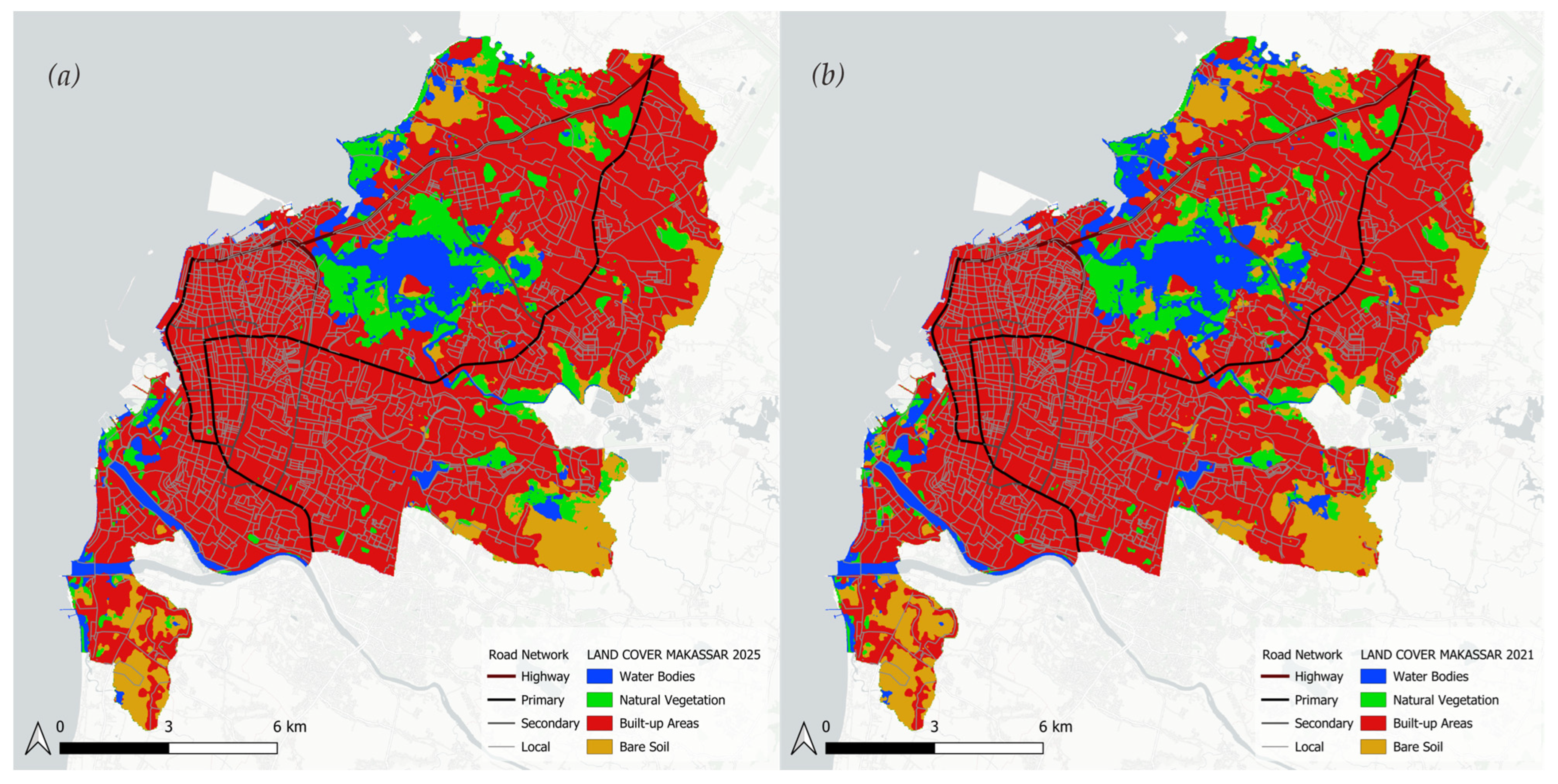
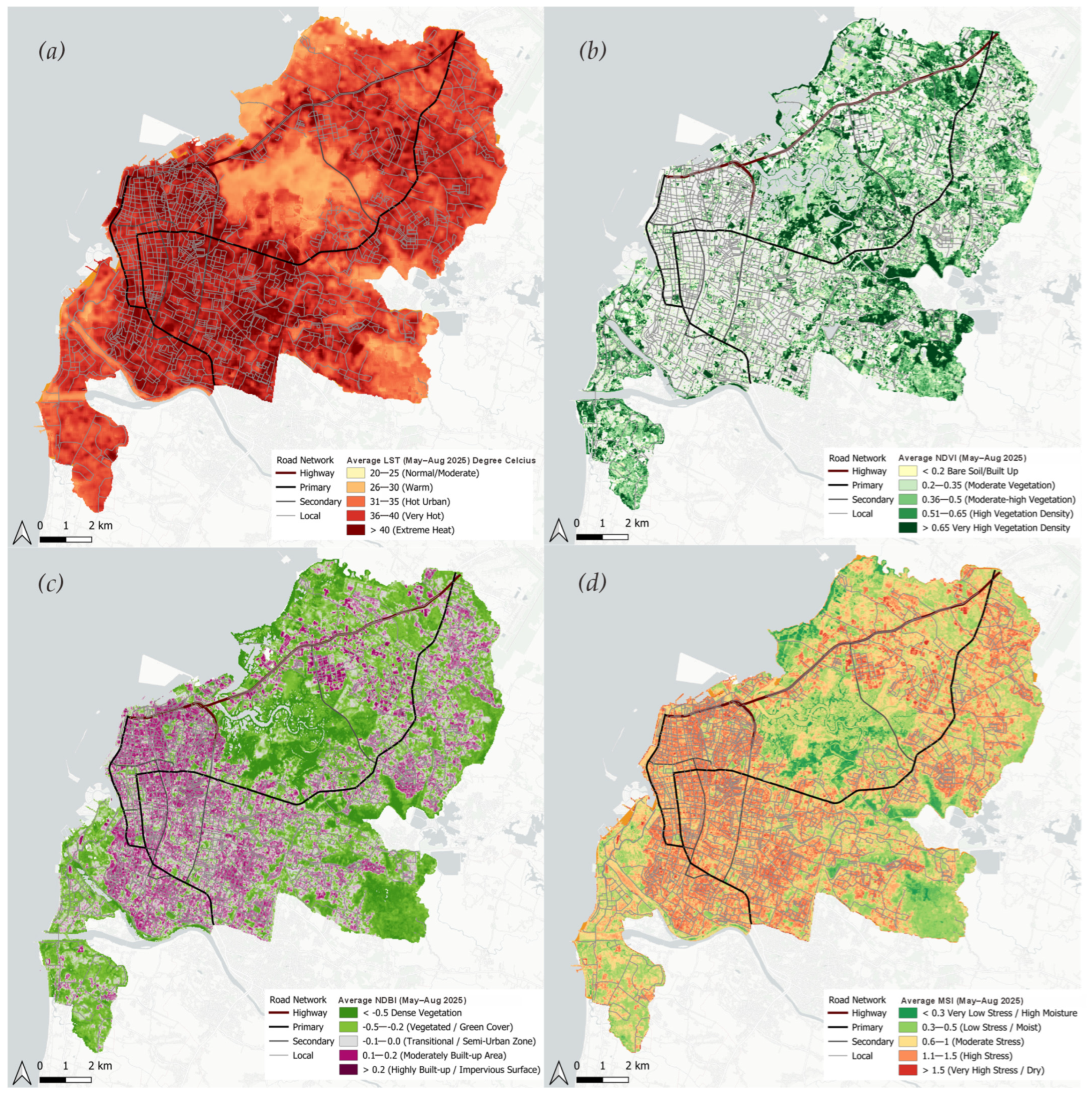
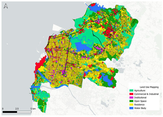
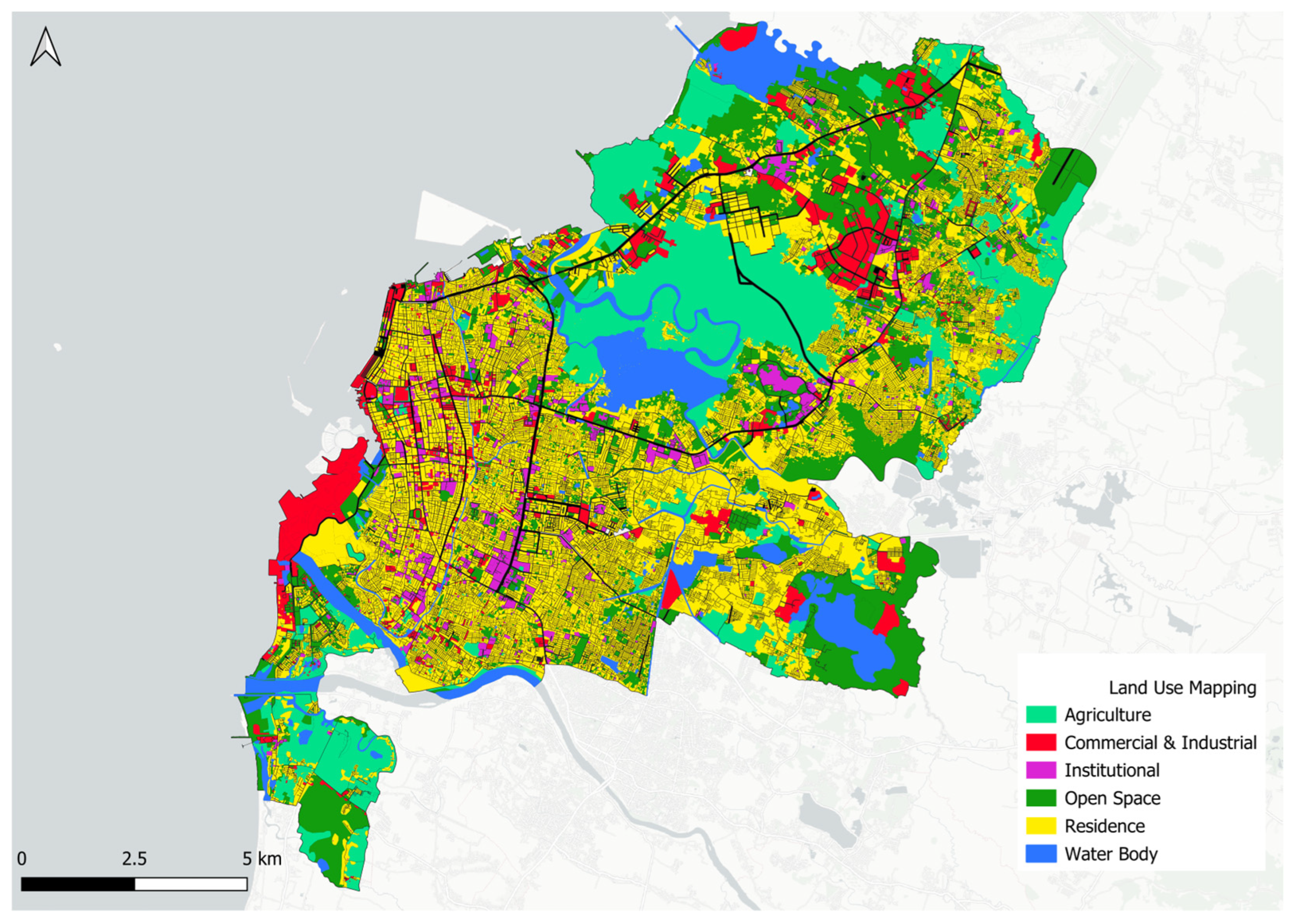
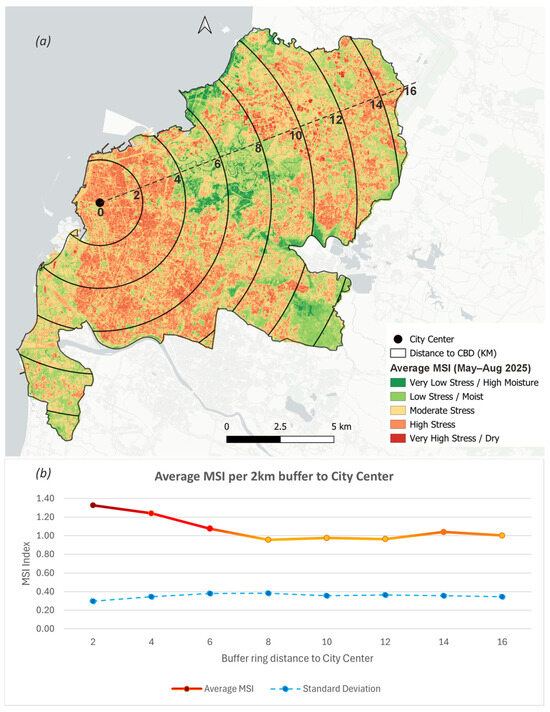
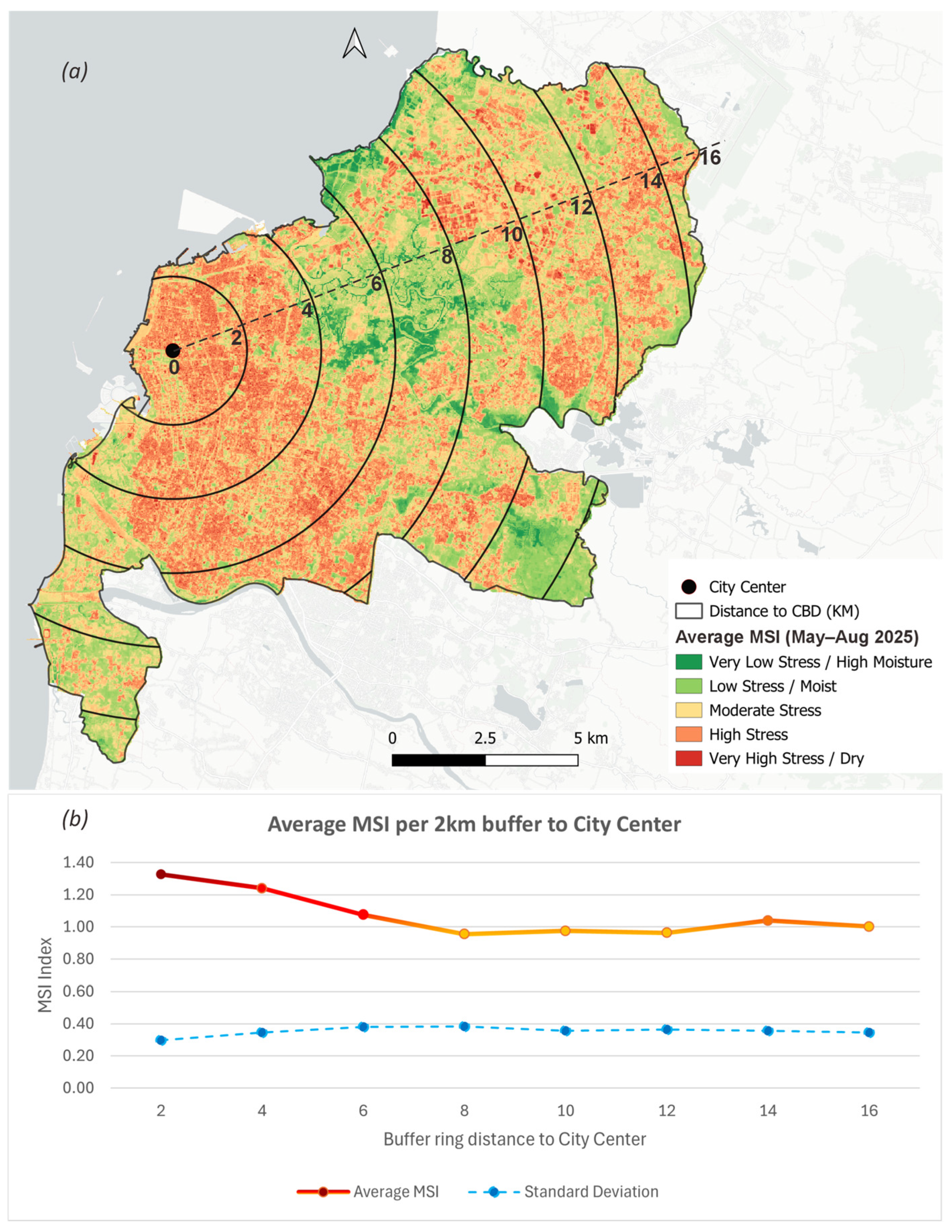
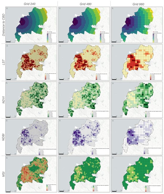
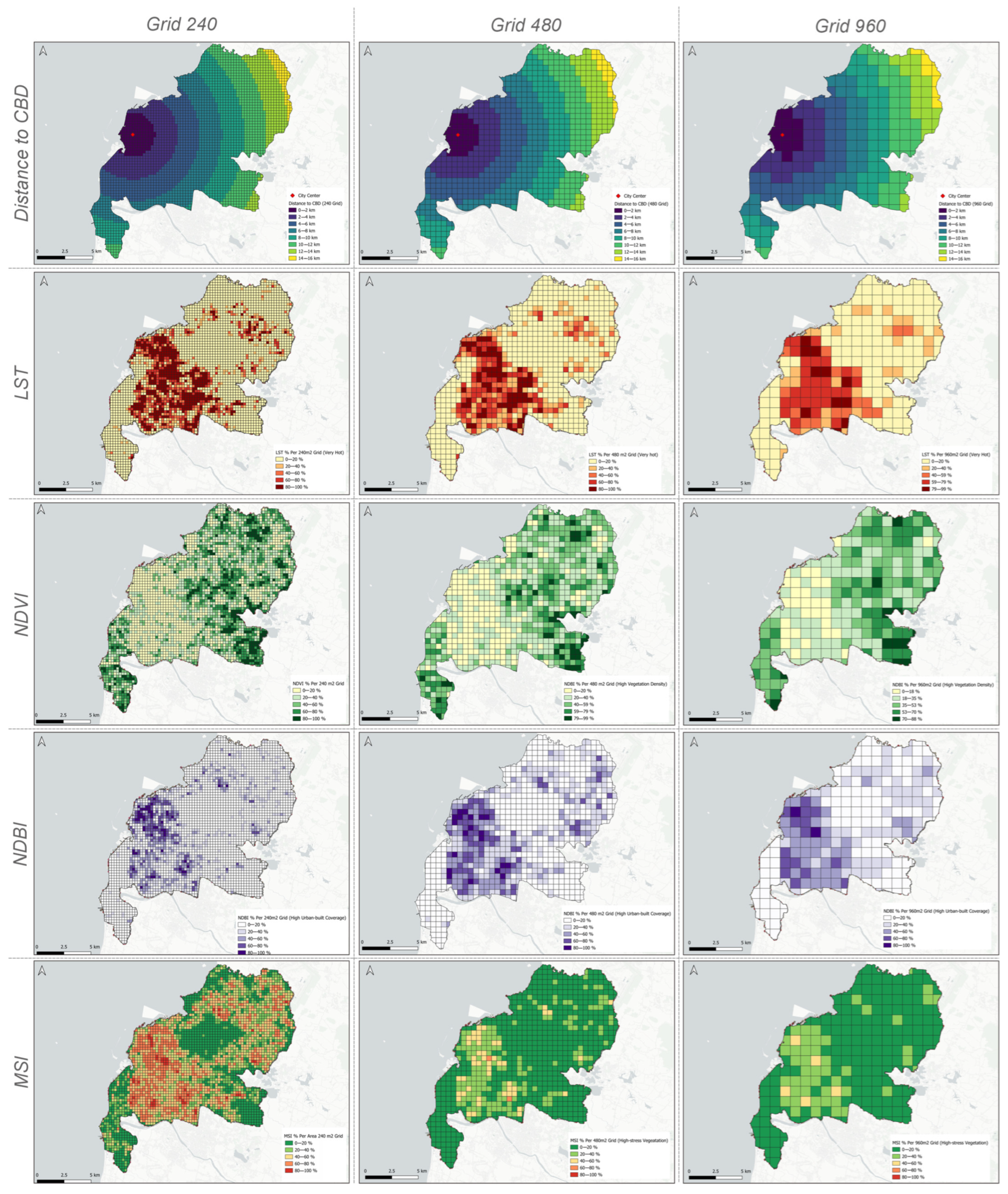
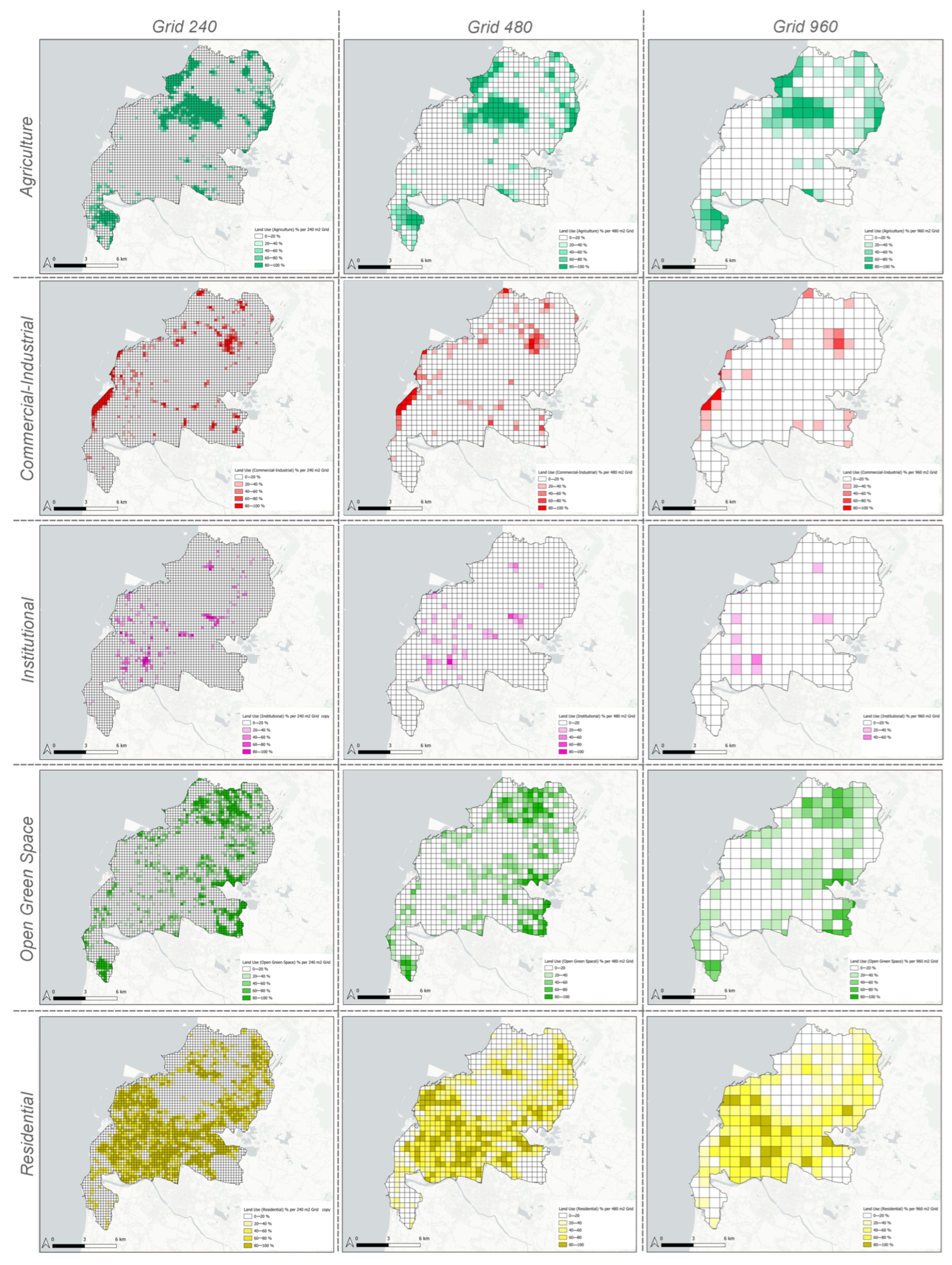
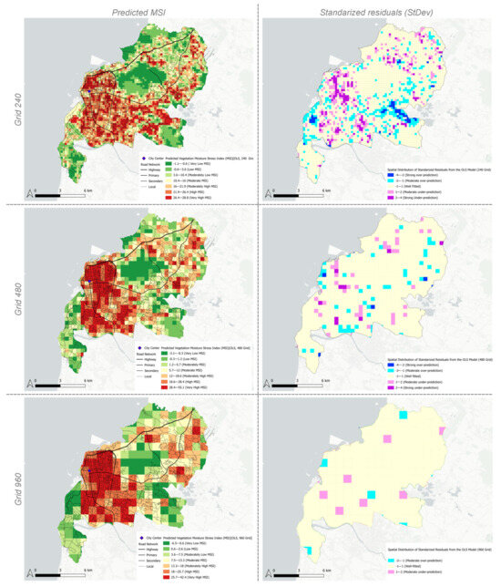
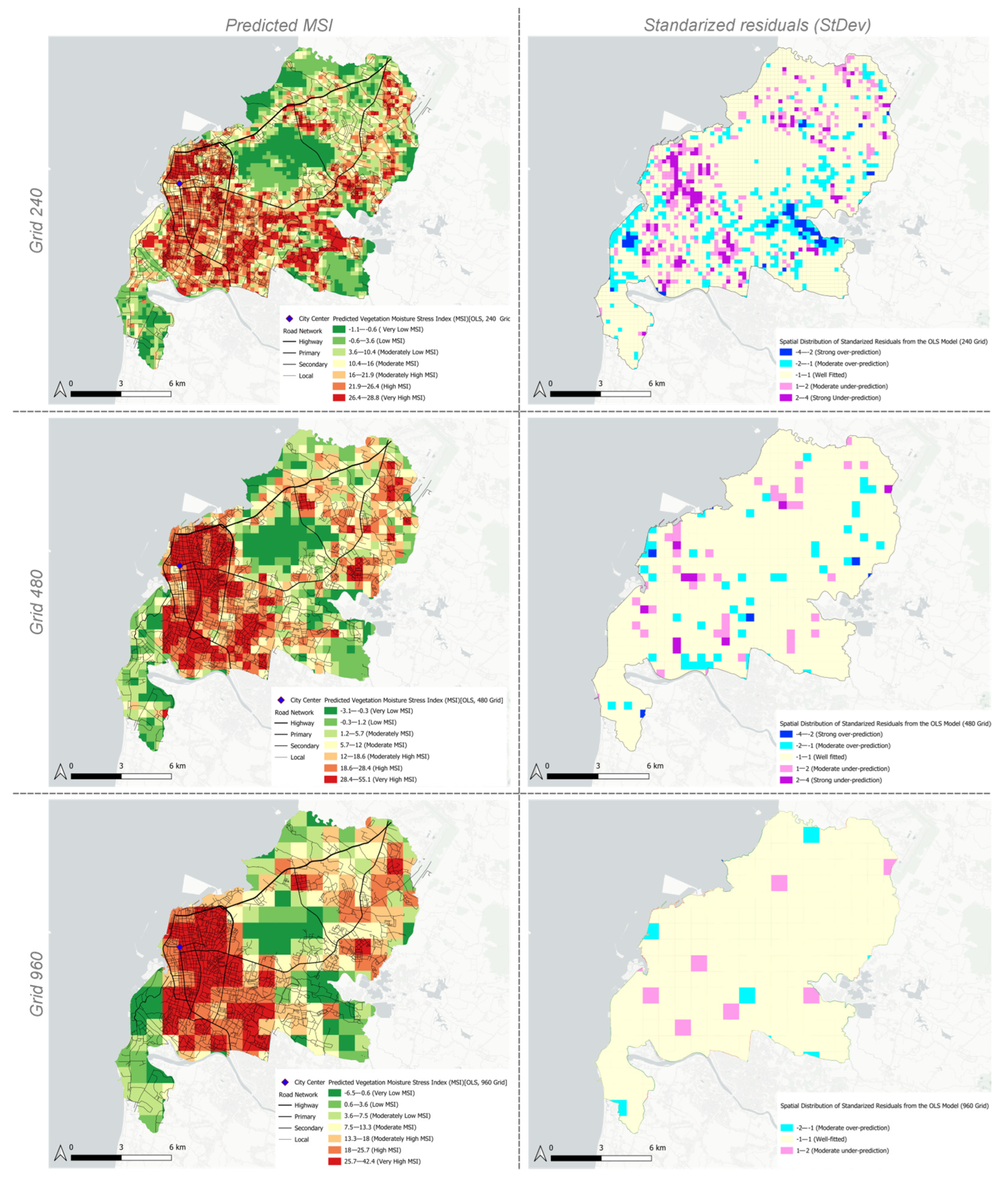
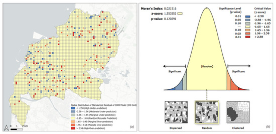
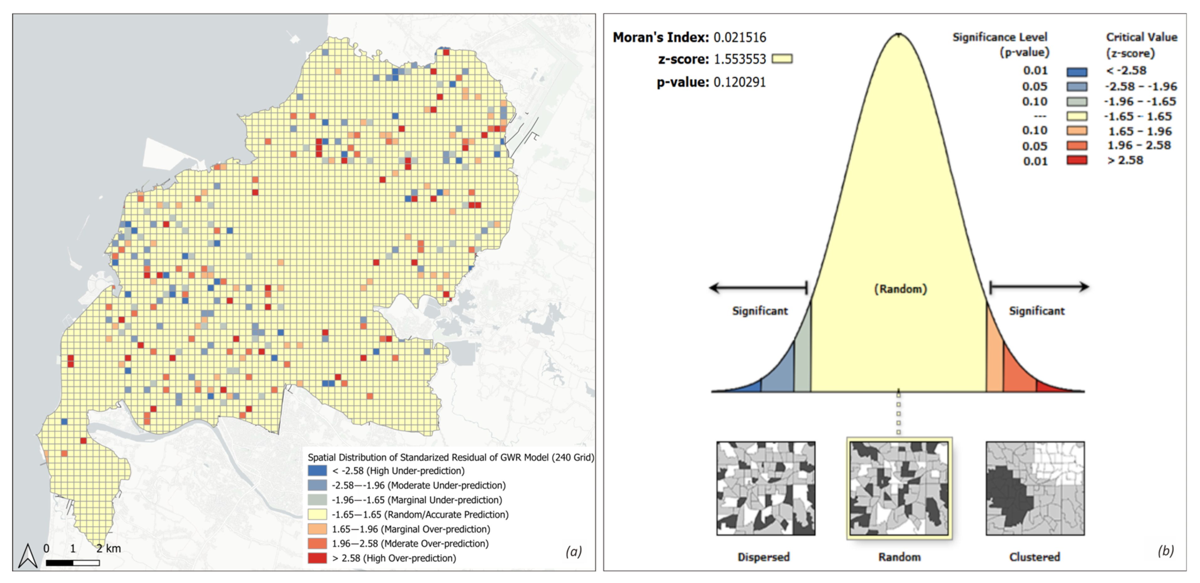
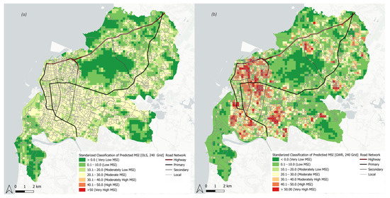
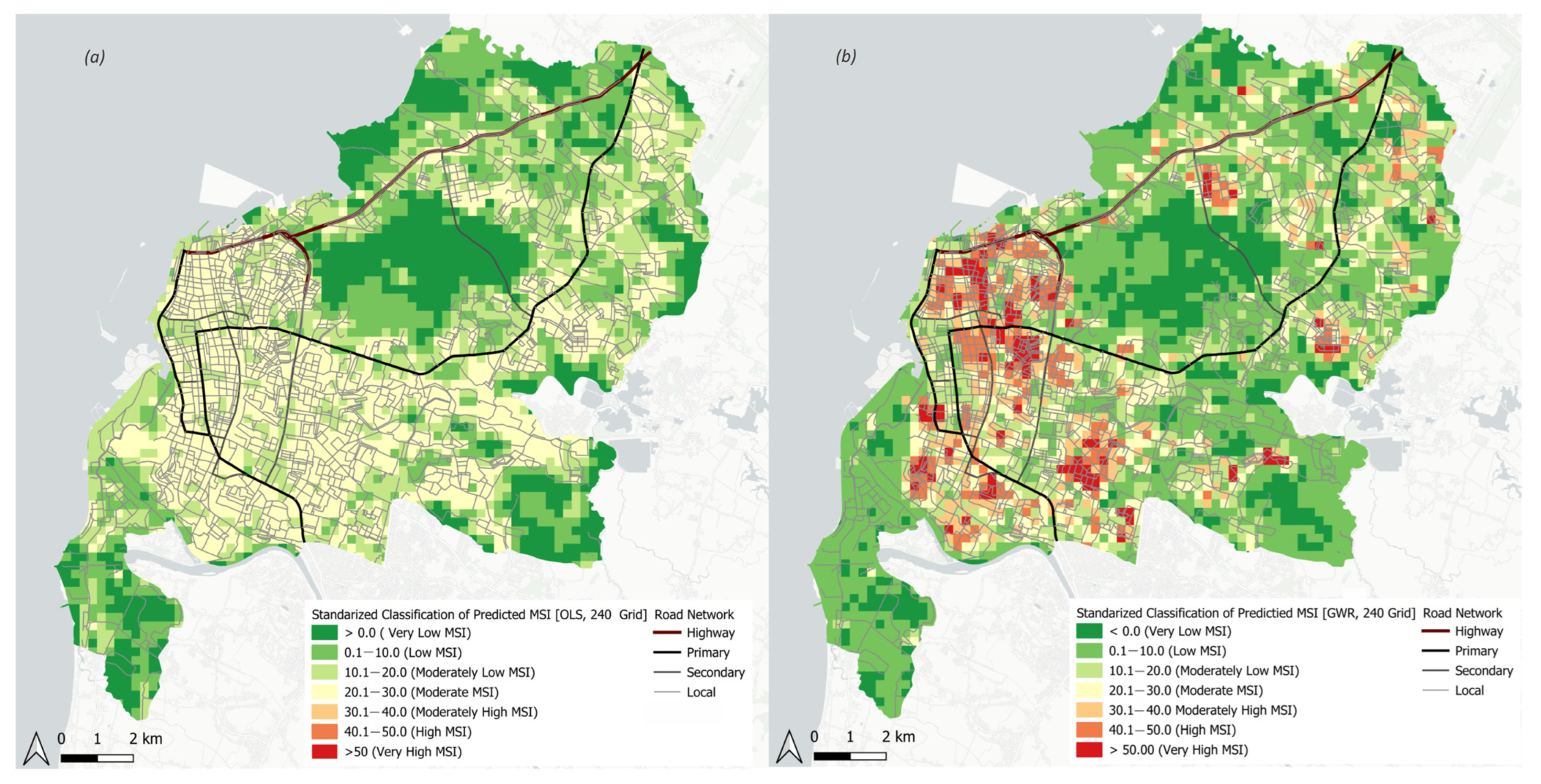
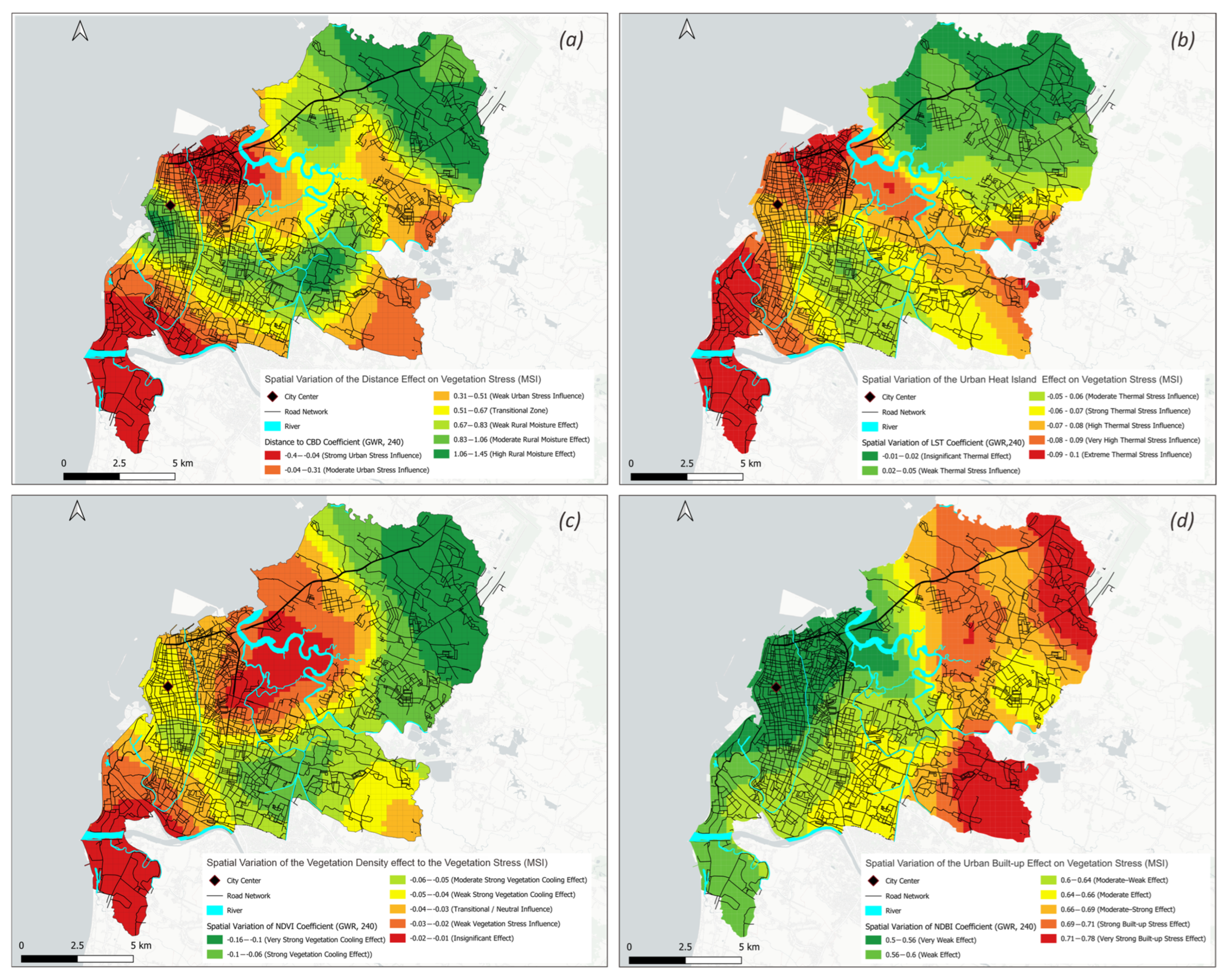
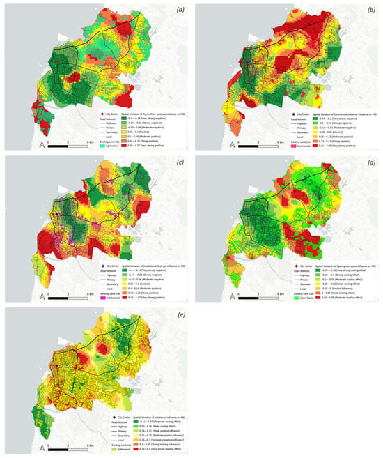
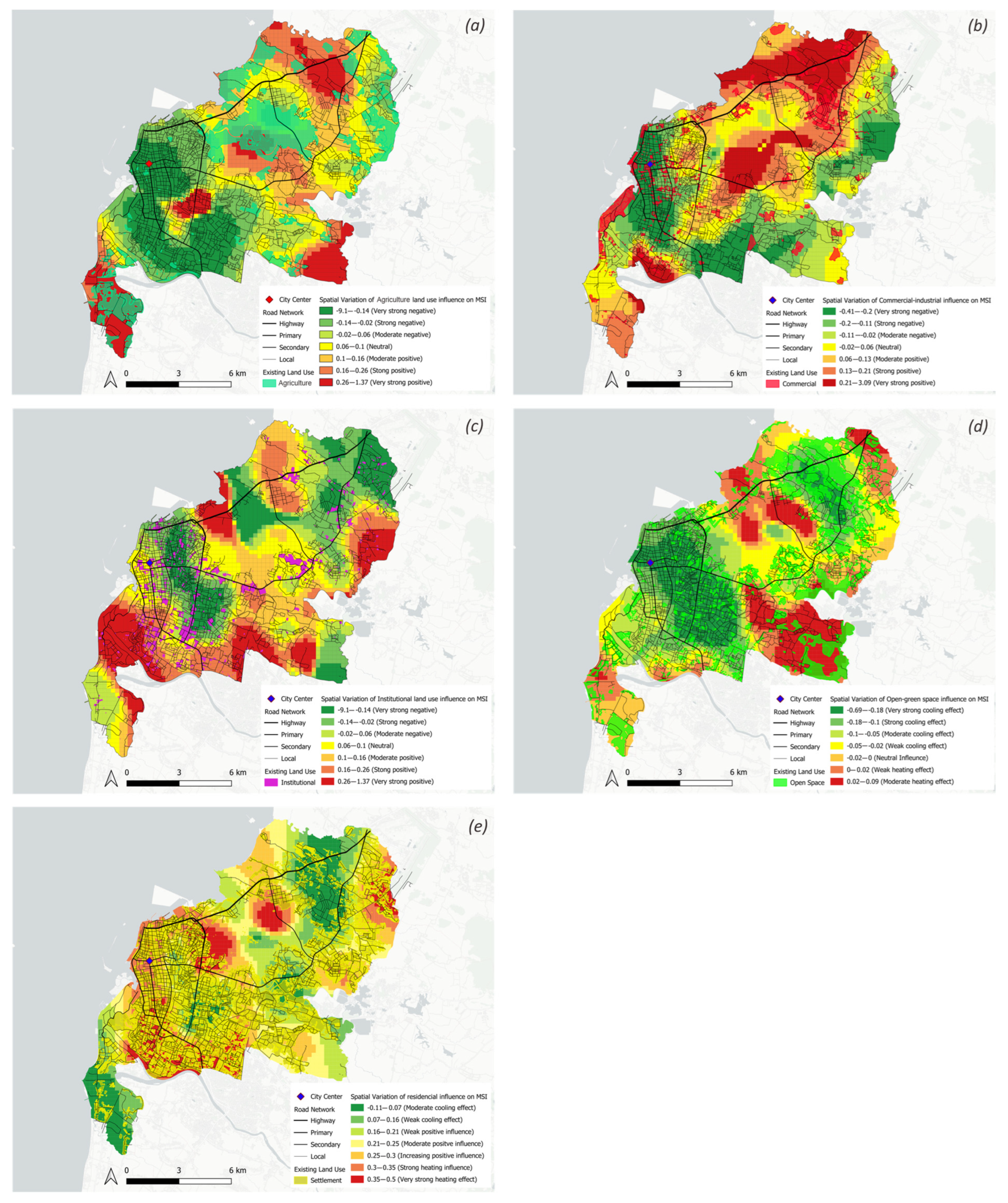
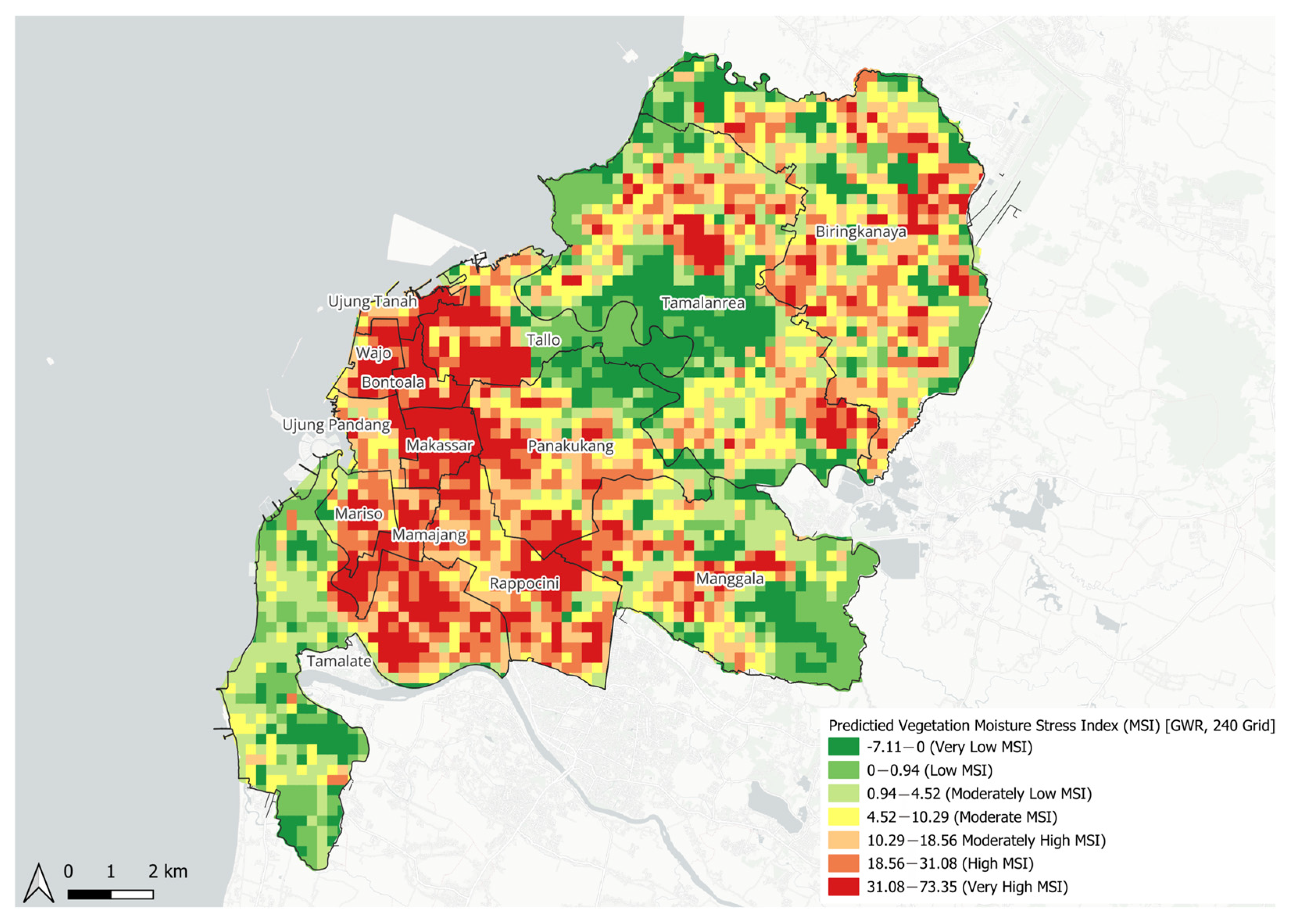

Disclaimer/Publisher’s Note: The statements, opinions and data contained in all publications are solely those of the individual author(s) and contributor(s) and not of MDPI and/or the editor(s). MDPI and/or the editor(s) disclaim responsibility for any injury to people or property resulting from any ideas, methods, instructions or products referred to in the content. |
© 2026 by the authors. Licensee MDPI, Basel, Switzerland. This article is an open access article distributed under the terms and conditions of the Creative Commons Attribution (CC BY) license.