Spatially Explicit Modeling of Urban Land Consolidation Potential: A New Bidirectional CA Framework for Reduction Planning Implementation

Abstract

Reduction planning has been implemented to mitigate urban sprawl in Chinese megacities. However, few studies have focused on the spatial implementation of urban land consolidation, and tools to estimate and simulate urban land consolidation are still lacking. To address the critical gap in urban land consolidation modeling, this study develops a bidirectional cellular automata model as a novel geospatial tool for quantifying consolidation potential and simulating future construction land dynamics under reduction planning. Our framework uniquely integrates high-resolution (30 m) simulation of simultaneous construction land expansion and reduction, overcoming limitations of conventional unidirectional models like the Future Land Use Simulation (FLUS) system, with validation confirming better accuracy. Using Beijing as a case study, the model identifies hotspots for land consolidation and, based on neighborhood-scale land transformation probabilities, delineates the spatial distribution of expansion and reduction zones, highlighting priority areas for consolidation. This provides the first operational tool for evidence-based urban reduction planning and land consolidation, offering a transferable methodology for optimizing land use efficiency and curbing disorderly expansion in megacities globally.

1. Introduction

Urbanization has led to rapid global urban land expansion, with a 130% increase between 1992 and 2013, particularly pronounced in Asia, which experienced the fastest growth rate [1]. Urban land provides the essential foundation for human socioeconomic activities, encompassing residential, economic, industrial, and transportation functions that drive economic development and population mobility [2,3,4]. However, low-density, poorly planned urban expansion—commonly referred to as urban sprawl—spreads across extensive areas of natural land, leading to inefficient land use [5,6,7]. For instance, a study analyzing the built-up land efficiency in China from 2005 to 2012 found a decline in input–output efficiency in most Chinese cities, with over half showing an oversupply of built-up land [8]. Urban sprawl has resulted in a range of negative externalities, including reduced biodiversity [9], decreased food production [10], intensified urban heat island [11,12], and structural changes in green spaces [13]. Therefore, addressing urban sprawl is essential and necessitates the implementation of urban containment strategies that promote sustainable urban development.

In response to these challenges, various urban containment strategies have been proposed to reshape urban development patterns [14,15,16]. Among these, urban growth boundaries (UGBs) have become a very common measure to control urban expansion in open spaces [17]. Areas within the boundary are designed to support a high density of urban services, effectively accommodating human activities [17,18]. Conversely, land outside the boundary is designated for natural resources and is protected from urban expansion [19]. Another well-known strategy is greenbelts, which are open spaces with forest or farmland surrounding a city to prevent excessive urban growth, protect ecological environment, and promote urban sustainable development [20,21,22]. Unlike UGBs, which delineate a boundary line separating urban and rural areas, greenbelts provide a physical buffer zone [14,20]. Besides these two major urban containment strategies, additional measures such as transit-oriented development [23], brownfield redevelopment [24,25], smart growth [26], and compact city planning [27] are also recognized as effective methods for managing urban sprawl worldwide.

Similar land consolidation strategies have also been implemented in China, which has undergone rapid urbanization, with urbanization rates increasing from 36% in 2000 to 60% in 2020 [28]. These strategies include cultivated land requisition–compensation balance [29], controls on construction land growth [30], and the redevelopment of inefficient urban land [31]. Although some progress has been achieved, significant challenges remain in effectively managing inefficient construction land [30,32]. To address these issues, more assertive land consolidation strategies are essential to reduce construction land, increase productivity, and improve the ecological environment.

One land consolidation approach currently being implemented in China is reduction planning, which aims to decrease the local city size and improve construction land efficiency of China [33]. In 2014, the former Ministry of Land and Resources issued the Guiding Opinions on Promoting Land Saving and Intensive Use, which introduced “Total Construction Land Control and Reduction Strategies” as a national priority [34]. This emphasis was reiterated in 2015 in the Overall Plan for the Reform of the Ecological Civilization System, issued by the Central Committee of the Communist Party of China and the State Council, which highlighted the “Control and Reduction of Total Construction Land” as a strategic objective [35]. Further, the 13th Five-Year Plan Outline for Land and Resources in 2016 strengthened this mandate, increasing the focus on land supplied from existing stock to enforce total construction land control and reduction [28].

At the local level, under the guidance of the national strategic framework, reduction planning has been actively explored in Chinese megacities [36]. For instance, the Beijing Urban Master Plan (2016–2035) sets the goal of reducing the scale of urban and rural construction land by 2035, emphasizing the need to decrease total land use, reduce more while increasing less, and optimize land-use structure. Following over 40 years of incremental land-use planning after the reform and opening-up policy, Beijing is gradually approaching the limits of its resource and environmental carrying capacity. Consequently, the city has experienced structural imbalances, traffic congestion, inadequate and unevenly distributed infrastructure, and rising housing prices—issues commonly referred to as “urban diseases” [37,38]. Therefore, there is an increasingly urgent need for land consolidation of construction land to support Beijing’s future sustainable development.

The current studies about land consolidation of China mainly focus on land consolidation in the rural areas. Land consolidation has been utilized as an integrated rural development tool that systematically optimizes land use patterns while addressing socio-spatial restructuring [39,40]. Existing studies have systematically examined the socio-economic impacts of rural land consolidation, with empirical findings demonstrating its capacity to enhance agricultural productivity and increase farmers’ income [41], improve rural living environments and public service delivery systems [42], and strengthen social cohesion. Furthermore, such initiatives facilitate coordinated urban–rural development and narrow the urban–rural income disparity [43], ultimately contributing to balanced regional socioeconomic progression. Scholarly investigations have also examined critical dimensions of land consolidation, including public participation and governance [44], as well as regional disparities in implementation efficacy under regionally differentiated contexts [45], thereby advancing theoretical frameworks for differentiated policy formulation.

However, research on land consolidation in China remains relatively limited across several key dimensions. Primarily, studies disproportionately focus on rural contexts, while systematic investigations into urban land consolidation amid rapid urbanization significantly lag behind. Secondly, current studies lack robust spatiotemporal analysis for critical areas such as land consolidation conflict diagnosis, land degradation risk early-warning, and multi-objective collaborative optimization, leaving fundamental questions about when, where, and how to implement consolidation reliant on empirical judgment rather than data-driven insights. Additionally, the insufficient adaptability of land consolidation technologies in high-density urban environments severely impedes the achievement of refined and comprehensive land management goals.

To address these challenges, we have developed the policy-oriented Bidirectional Cellular Automata Model to identify urban land consolidation potential while simulating expansion and land consolidation dynamics, aiming to advance evidence-based land governance through enhanced spatiotemporal diagnostics and high-density adaptability. We first quantified land cover change in Beijing (2016–2020) under the construction land reduction strategy using Sentinel-2 imagery, available during 2015 to 2025, processed via the Google Earth Engine (GEE) platform. Subsequently, we developed bidirectional GEE-CA (Google Earth Engine-Cellular Automata), a significant advancement over the original GEE-CA model [46]. While the predecessor solely projected urban expansion, our enhanced model explicitly incorporates dual-directional dynamics, simultaneously simulating construction land consolidation (reduction) and targeted expansion within planning constraints. To validate the model, we calibrated it with 2016–2020 construction land data and generated 2024 predictions. These outputs were rigorously tested against observed 2024 land patterns, confirming the model’s capability to replicate reduction-driven transitions. Finally, leveraging Beijing’s 2035 Urban Master Plan objectives, we deployed the Bidirectional GEE-CA to project high-resolution (30 m) construction land scenarios under continuous reduction governance, thereby operationalizing evidence-based spatial diagnostics for land-use optimization. This study has three objectives: (1) to analyze the expansion and reduction of construction land in Beijing from 2016 to 2020 using land use classification data; (2) to develop a bidirectional GEE-CA model capable of simultaneously simulating both expansion and reduction of construction land, incorporating Beijing’s dynamic changes; (3) to identify potential areas for future construction land reduction through repeated simulations with the bidirectional GEE-CA model.

2. Methods

2.1. Study Area

As the second-largest city in China after Shanghai, Beijing has experienced tremendous urbanization, especially in the 21 century (Figure 1). The rapid expansion of urban and rural construction land—from 2397 km² in 2005 to 2921 km² in 2015—highlighted the urgent need for land consolidation to counteract inefficient sprawl. To improve urban governance systems, address megacity challenges, and advance sustainable development, the Beijing Urban Master Plan (2016–2035) explicitly adopts land consolidation as a key mechanism, targeting a reduction of total construction land to approximately 2760 km² by 2035. This involves systematic reclamation of inefficient land through a city-wide demolition-to-occupation ratio of 1:0.7 to 1:0.5. As the pioneer in implementing such a consolidation-driven reduction plan, Beijing provides an ideal case for analyzing current land dynamics and simulating future changes under integrated spatial governance frameworks.

2.2. Land Cover Classification

2.2.1. Data Preprocessing

Multi-spectral Sentinel-2 Level 1C images [47], with 13 spectral bands and a high spatial resolution of 10 m, were used for the years 2016, 2020, and 2024 and are available on GEE [48]. To mitigate the influence of seasonal variance of spectral characteristics, we first filtered the Sentinel-2 images for each research year (2016, 2020, and 2024) to include only those acquired between March and October. Subsequently, we excluded images with a cloud pixel percentage exceeding 20% to ensure the quality of the dataset. Furthermore, we employed the QA60 band to mask out clouds and cirrus pixels in images with less than 20% cloud coverage to acquire clearer Sentinel-2 images. Finally, we adopted the median value [49,50,51] of each band to represent their average spectral characteristics, ensuring robustness against potential noise.

To optimize the GEE classification model, it is crucial to limit the number of features by selecting the most relevant ones, thereby reducing computational processing costs [50]. Consequently, we prioritized the selection of spectral bands significant for land cover classification. A total of nine original spectral bands (B2–B8, B8A, and B11) were selected for the subsequent land cover classification, based on previous research. Additionally, spectral indices derived from these bands are frequently utilized as essential information for enhancing classification accuracy [47,49,52]. Three spectral indices were explicitly incorporated as classification features: $\mathrm{N}\mathrm{D}\mathrm{V}\mathrm{I}$ (normalized difference vegetation index) [47], $\mathrm{N}\mathrm{D}\mathrm{W}\mathrm{I}$ (normalized difference water index) [49], and $\mathrm{N}\mathrm{D}\mathrm{B}\mathrm{I}$ (normalized difference built-up index) [52]. The equation of each index was provided as follows:

$$\mathrm{N}\mathrm{D}\mathrm{V}\mathrm{I}={\displaystyle \frac{NIR-Red}{NIR+Red}}$$

(1)

$$\mathrm{N}\mathrm{D}\mathrm{W}\mathrm{I}={\displaystyle \frac{Green-NIR}{Green+NIR}}$$

(2)

$$\mathrm{N}\mathrm{D}\mathrm{B}\mathrm{I}={\displaystyle \frac{SWIR1-NIR}{SWIR1+NIR}}$$

(3)

where $Green$, $Red$, $NIR$, and $SWIR1$ refers to Band 3, Band 4, Band 8, and Band 11 of sentinel-2 images, respectively.

2.2.2. Classification

Various machine learning algorithms have been employed for land cover classification using GEE. Among these, the random forest (RF) algorithm has demonstrated superior performance compared to other classifiers, owing to its high accuracy, robustness, and ease of parameterization [47,49,50]. Therefore, we applied the RF classifier in GEE to create land cover classifications for Beijing in 2016, 2020, and 2024 (

Table 1. The training and testing samples of each land cover type in 2016, 2020, and 2024.

Land Cover Types	2016		2020		2024
	Training	Testing	Training	Testing	Training	Testing
Construction	139	61	140	75	159	61
Farmland	58	27	42	18	36	14
Water	24	10	22	22	22	13
Forest	46	36	41	19	43	37
Grassland	2	1	4	1	2	1
Bare land	5	0	1	0	3	0

).

To briefly represent the existing land cover types in Beijing, we classified the data into six categories: construction land, farmland, water, forest, grassland, and bare land. For each year, we collected over 400 samples, ensuring that more than half of the selected samples represented construction land. From this dataset, 70% of the samples were randomly designated for training the land cover classification model, while the remaining 30% were reserved for testing its accuracy. Validation of the classifications results was conducted using independent datasets.

2.2.3. Accuracy Assessment

The differences between the testing data and the land cover classifications were exhibited using a confusion matrix. The overall accuracy estimations and kappa coefficients were employed to demonstrate the accuracy of land cover classification for each year [47,49,50].

Additionally, given that this study emphasizes construction land, we randomly generated 100 sample points for construction land each year and imported them into Google Earth for comparison with historical imagery. This approach was implemented each year to validate the accuracy of the construction land classification by assessing metrics such as overall accuracy and user’s accuracy.

2.2.4. Further Processing

We reclassified the land cover types for both years, grouping farmland, water, forest, grassland, and bare land as non-construction land. This approach effectively condenses the land cover data into two primary categories: construction land and non-construction land. Subsequently, we generated the land cover transition map by performing an overlay of the 2016 and 2020 datasets to identify all pixels with four possible transition states: non-construction land to non-construction land (NN), construction land to construction land (CC), non-construction land to construction land (NC), and construction land to non-construction land (CN).

2.3. Bidirectional GEE-CA Framework

2.3.1. Original GEE-CA

The original GEE-CA is a newly developed online urban expansion simulation tool with a 30 m spatial resolution [46]. It integrates several key components, including the preprocessing of spatial factor datasets, the prediction of future urban land demand, the implementation of CA iteration for urban expansion simulation, and the assessment of global simulation accuracy on the GEE platform. The development probability used in GEE-CA includes occurrence probability, neighborhood intensity, development constraints, and stochastic factor.

Urban expansion likelihood is shaped by multiple spatial determinants. Existing research has underscored a variety of natural and socioeconomic drivers, including terrain elevation data, central urban zones, primary and secondary road networks, water bodies such as rivers, lakes, and coastal areas, as well as transportation hubs like airports [46,53,54]. The associations between the likelihood of urban development and these spatial variables tend to be nonlinear characteristics. Random forest algorithms are capable of efficiently handling extensive datasets with numerous inputs. To rapidly analyze large-scale spatial drivers, we employed the random forest model to build the connection between the spatial probability of urban occurrence and the factors influencing urban growth. The number of decision trees in the random forest model was set to 100:

$$p_{incre, suit}=F_{incre }(x_1, x_2, \dots ,x_9)$$

(4)

$$p_{incre, neigh}={\displaystyle \frac{\sum _{i,j}{S}_{i, j}}{n \ast n}}$$

(5)

$$p_{incre, restrict}=water \mathit{⨂} slope \mathit{⨂} policy$$

(6)

$$p_{random}=1+{(-\mathit{ln}\gamma )}^{\alpha }$$

(7)

$$p_{incre}=p_{incre, suit} \ast p_{incre, neigh} \ast p_{incre, restrict} \ast p_{random}$$

(8)

$$S_{t, i, j}=\left\{\begin{array}{c}1, if p_{incre}>p_{incre, thres}\\ 0, if p_{incre} \le p_{incre, thres}\end{array}\right.$$

(9)

where $p_{incre, suit}$ refers to the construction land expansion occurrence probability; $F_{incre}$ refers the trained random forest model for construction land expansion; and DEM ($x_1$), Distance to airports ($x_2$), Distance to centers ($x_3$), Distance to lakes ($x_4$), Distance to main roads ($x_5$), Distance to ocean ($x_6$), Distance to ordinary roads ($x_7$), Distance to rivers ($x_8$), and Nighttime light ($x_9$) refer to selected variables of construction land expansion driving factors. The specific variables and the relative importances of these variables on construction land expansion using random forest algorithm can be found in

Table 2. The relative importances of selected variables of construction land expansion and reduction using the random forest algorithm.

Variables	Expansion	Reduction
DEM ($x_1$)	0.14	0.11
Distance to airports ($x_2$)	0.11	0.12
Distance to centers ($x_3$)	0.10	0.11
Distance to lakes ($x_4$)	0.10	0.09
Distance to main roads ($x_5$)	0.10	0.11
Distance to ocean ($x_6$)	0.11	0.11
Distance to ordinary roads ($x_7$)	0.12	0.11
Distance to rivers ($x_8$)	0.11	0.10
Nighttime light ($x_9$)	0.11	0.14

. $p_{incre}$ refers to the construction land expansion probability, $p_{incre, suit}$ refers to the construction land expansion occurrence probability, $p_{incre, neigh}$ refers to the construction land expansion neighborhood intensity, $n$ refers to the window size of neighborhood calculation, which was set to 5, $S_{i, j}$ refers to the status of cellular $i, j$ within the window, 1 refers to construction land, 0 refers to non-construction land. $p_{incre, restrict}$ refers to construction land expansion development constraints, water refers to the water constraint which means construction land expansion will not occur in the water land, slope refers to the slope constraint which means construction land expansion will not occur in the high slope land, policy refers to the areas which were recommended to develop in the Beijing policy. $p_{random}$ refers to construction land stochastic factor, $\gamma$ refers the stochastic factor ranging from 0 to 1 and $\alpha$ refers the parameter controlling the random scale. $S_{t, i, j}$ refers to the status of cellular $i, j$ at time $t$, 1 refers to urban, 0 refers to non-urban. $p_{incre, thres}$ is determined by first ranking $p_{incre}$ of each cell from highest to lowest, then it accumulates total m cells until meeting the urban expansion size; $p_{incre, thres}$ is equal to the $p_{incre}$ value of cell m, which was derived from the demand of future construction land expansion.

Compared to traditional urban expansion simulation models, the GEE-CA model offers advantages of faster processing speed, higher spatial resolution (up to 30 m), and the flexibility to be applied across various scales and regions. Additionally, it is capable of simulating multiple future development scenarios. However, the original GEE-CA is exclusively designed to model urban expansion or growth scenarios exclusively, which limits its direct applicability to this study. As such, the model requires further refinement and modifications to meet the specific needs of construction land reduction in this research.

2.3.2. Bidirectional GEE-CA

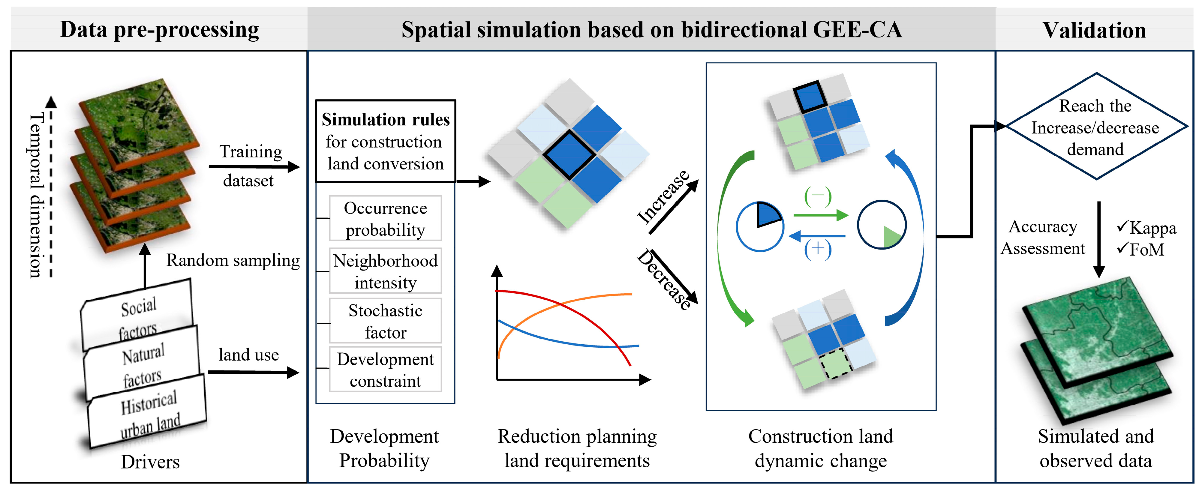
The core objective of land consolidation-driven reduction planning is to achieve a net decrease in total construction land while allowing for structural adjustments in land allocation. To operationalize this, we integrated an urban land consolidation module into the GEE-CA model, enabling simultaneous simulation of construction land expansion and consolidation-led reduction. This resulted in the development of our bidirectional GEE-CA model (Figure 2).

In the construction land expansion module, we preserved the original GEE-CA structure, utilizing natural and socioeconomic drivers, including DEM ($x_1$), Distance to airports ($x_2$), Distance to centers ($x_3$), Distance to lakes ($x_4$), Distance to main roads ($x_5$), Distance to ocean ($x_6$), Distance to ordinary roads ($x_7$), Distance to rivers ($x_8$), and Nighttime light ($x_9$) to model development suitability via random forest algorithms [46,55]. The selection of these variables (Table 2) was informed by existing studies that have demonstrated the capacity of such drivers to enhance the accuracy of future simulations [46,56]. Among these, nighttime lights can be regarded as an indicator of land use efficiency to a certain extent. The relative importance of variables for simulating construction land expansion and reduction, as quantified by the Random Forest (RF) algorithm, is summarized in Table 2. The results demonstrate that the selected variables exhibit comparable importance levels in both expansion and reduction simulations.

We reclassified the construction land transition map, assigning a value of 1 to the pixels representing construction land expansion (NC), and a value of 0 to the other three transition types (NN, CC, and CN). The neighborhood intensity, development constraints, and stochastic factor were consistent with the methodology outlined by Meng et al. [46]. Then, the development probability of construction land expansion was derived from the occurrence probability, neighborhood intensity, development constraints, and stochastic factor. The potential areas for future construction land expansion were jointly determined by the development probability of each pixel and the future expansion demand.

In the newly integrated construction land reduction module, we employed the same set of driving factors used in the urban expansion module to simulate construction land reduction occurrence probability, with the core premise being the recognition that the same socioeconomic and geographical factors exert opposite effects on urban expansion and reduction (Table 2). For example, high nighttime light intensity typically indicates robust economic activity and strong demand, serving as a positive driver for urban expansion. Conversely, low nighttime light intensity suggests insufficient economic vitality and low land-use efficiency, acting as a key indicator for identifying potential reduction zones. Proximity to city centers or major roads, due to high locational value and accessibility, strongly attracts construction activities (expansion). In contrast, areas distant from these elements, owing to their locational disadvantages, are more likely to be prioritized for consolidation (reduction) during industrial restructuring and functional decentralization. Our model does not simply apply the same factors in reverse for simulating reduction. Instead, it employs machine learning (random forest) to independently learn two distinct sets of relationships from historical data: one between the driving factors and the probability of expansion, and another between the same factors and the probability of reduction. This approach allows the model to capture the divergent socioeconomic logics that underpin urban expansion and reduction, respectively.

For urban reduction simulation, we reclassified the construction land transition map by assigning a value of 1 to the pixels representing the CN transition and a value of 0 to the other three transition types (NN, CC, and NC). The neighborhood intensity in this module considered the intensity of non-construction land; the higher the intensity of non-construction land, the greater the likelihood of its conversion to non-construction land. In addition to conventional factors such as water availability and slope, we also included roads, particularly highways connecting peripheral towns, as part of the development constraints. The stochastic factor influencing urban reduction was the same as the inverse of the stochastic factor used in the construction land expansion module.

$$p_{decre, suit}=F_{decre}(x_1, x_2, \dots ,x_9)$$

(10)

$$p_{decre, neigh}={\displaystyle \frac{\sum _{i,j}(1-S_{i, j})}{n \ast n}}$$

(11)

$$p_{decre, restrict}=slope \mathit{⨂} road \mathit{⨂} policy$$

(12)

$$p_{decre}=p_{decre, suit} \ast p_{decre, neigh} \ast p_{decre, restrict} \ast p_{random}$$

(13)

$$S_{t, i, j}=\left\{\begin{array}{c}0, if p_{decre}>p_{decre, thres}\\ 1, if p_{decre} \le p_{decre, thres}\end{array}\right.$$

(14)

where $p_{decre, suit}$ refers to the construction land reduction occurrence probability, $F_{decre}$ refers the trained random forest model for construction land reduction, $x_1$, $x_2$, … $x_9$ refer to selected variables of driving factors mentioned before (the relative importances of these variables on construction land reduction using random forest algorithm can be found in Table 2), $p_{decre, neigh}$ refers to the construction land reduction neighborhood intensity, n refers the window size of neighborhood calculation, which was set to 5, $S_{i, j}$ refers the status of cellular $i, j$ within the window size, 1 refers to construction land, 0 refers to non-construction land, $p_{decre, restrict}$ refers to construction land reduction development constraints, slope refers to the slope constraint which means construction land reduction will tend to occur in the high slope land, road refers to the road constraint which means construction land reduction will not occur in the roads, policy refers to the areas which were not recommended to develop in the Beijing policy, $p_{decre}$ refers to the construction land reduction probability, $S_{t, i, j}$ refers to the status of cellular $i, j$ at time $t$, 1 refers to urban, 0 refers to non-urban. $p_{decre, thres}$ is determined by first ranking $p_{decre}$ of each cell from highest to lowest, then it accumulates the total n cells until meeting the urban reduction size, $p_{decre, thres}$ is equal to the $p_{incre}$ value of cell m, which was derived from the demand of future construction land reduction.

Our approach constitutes a significant methodological extension of the CA framework for land-use modeling. While building upon classical CA concepts, our model’s key innovation lies in its operationalization of bidirectional, policy-oriented transitions to address the specific need for simulating net land reduction, a capability not found in conventional expansion-only CA models.

2.3.3. Simulation Workflow

The bidirectional GEE-CA model operates through an integrated workflow that simulates construction land expansion and reduction simultaneously within each iterative time step. This process ensures that the net change in construction land aligns with the predefined planning targets. The computational workflow, summarized in Figure 2, proceeds as follows:

(1) Initialization

The simulation begins by loading the initial land-use map at time t₀, along with the spatial driver datasets, constraint layers, and model parameters. The total number of iterations T is set to 15, corresponding to the simulation period from 2020 to 2035. The target quantities for construction land expansion (122 km²) and reduction (195 km²) for the entire period are imported as model inputs, derived from the Beijing Urban Master Plan (2016–2035).

(2) Iterative Simulation Loop

For each time step t from 1 to T:

a. Parallel Probability Calculation: For every cell in the study area, the model calculates two independent development probabilities in parallel:

Expansion Probability: For non-urban cells, the model computes the suitability for expansion using Equation (4), the neighborhood intensity (5 × 5) using Equation (5), and applies the development constraints for expansion via Equation (6). The final expansion probability is then synthesized using Equation (8).

Reduction Probability: For urban cells, the model simultaneously computes the suitability for reduction using Equation (10), the neighborhood intensity (based on non-urban land 5 × 5) using Equation (11), and applies the distinct set of constraints for reduction via Equation (12). The final reduction probability is synthesized using Equation (13).

b. Sequential and Mutually Exclusive Transition Rule: This step constitutes the core integration mechanism that ensures the logical consistency of simultaneous expansion and reduction. To prevent a cell from being considered for both expansion and reduction within the same iteration—a logical impossibility—the model processes the two transitions sequentially in a mutually exclusive manner.

Threshold Determination: First, the expansion demand for the current iteration is used to determine the expansion threshold by ranking all values of non-urban cells. Similarly, the reduction demand for the iteration is used to determine the reduction threshold by ranking all values of urban cells.

Priority to Reduction: The model first processes all urban cells for potential reduction. For each urban cell, if its reduction probability exceeds the reduction threshold, it is marked for conversion from construction land to non-construction land (transition from 1 to 0). Crucially, once a cell is marked for reduction, it is removed from the pool of cells eligible for expansion in the current iteration.

Subsequent expansion on stable non-urban land: After all potential reduction transitions have been identified and the land-use map is conceptually updated, the model then processes non-urban cells for expansion. A non-urban cell is converted to urban (transition from 0 to 1) if it was not an urban cell at the start of the iteration (i.e., it is not a cell that was just reduced) and its expansion probability exceeds the expansion threshold.

c. Synchronous Map Update: After all cells have been evaluated, the land-use map is updated synchronously based on the transition decisions made in step 2b. This ensures that the new spatial configuration at time t + 1 reflects the simultaneous processes of expansion and reduction.

(3) Termination and Output

The loop continues until the total number of iterations T is completed. The model outputs the final simulated land-use map for the target year 2035, which achieves a net reduction in construction land area as mandated by the planning quota while realistically capturing the spatial dynamics of both expansion and reduction.

2.3.4. Model Accuracy Validation and Sensitivity Analysis

We used the model to predict the construction land conditions for 2024 and compared the predicted results with the actual construction land classification data for 2024. The model validation consists of two steps: (1) to validate comparability of this model, we used the Kappa coefficient and the Figure of Merit (FoM) to assess model accuracy [46], and the results were compared horizontally with those of similar studies (focused on different regions) to assess the model’s generalizability; (2) to validate the reliability of this model, the same data and objectives were input into FLUS, a widely used land use simulation model, and the simulation results (Kappa and FoM) of Beijing generated by our model were directly compared with those of FLUS to further verify robustness.

During the model’s operation, certain parameters defined at the initial stage of the study influence the simulation outcomes, such as neighborhood size, number of iterations, and the quantity of decision trees in the random forest model. In the results presented in the main text, the neighborhood size was set to 5 × 5, the iteration count to 15, and the number of random forest decision trees to 100 (referred to as the baseline scenario). To evaluate sensitivity of these parameters on the simulation results, we modified the neighborhood size to 3 × 3 and 7 × 7, the iteration count to 10 and 20, and the number of decision trees to 90 and 110, respectively. In each simulation run, only one parameter was altered while the others remained consistent with the baseline values, and 100 simulations of construction land change were performed for each variation, yielding six sets of sensitivity analysis results. Finally, the outcomes of the 100 simulations under each modified parameter setting were aggregated to compute the probabilities of construction land expansion and reduction. These aggregated results were then compared with those of the baseline scenario (results from Section 2.3.5). Smaller discrepancies between the modified and baseline results indicate the less influence of parameter changes on the simulation outcomes, whereas larger discrepancies suggest a greater impact.

2.3.5. Future Simulation

After confirming the reliability of our bidirectional GEE-CA model, we conducted a simulation of the changes in built-up land for the year 2035, using 2020 as the baseline year. Based on the requirements of the urban planning in Beijing regarding the overall reduction of construction land and the demolition-to-construction ratio, we ultimately set the construction land expansion and reduction for 2035 compared to 2020 at 122 km² and 195 km², respectively. Due to the inherent randomness in the results of future simulations, we performed a total of 100 simulations, overlaying the results to calculate the probabilities of construction land expansion and reduction for each grid cell.

Two widely utilized spatial autocorrelation methods, the Moran’s I index and the Local Spatial Association (LISA) index, were employed to analyze the simulation results. This analysis evaluated the spatial distribution characteristics of the potential for construction land remediation. The Moran’s I index ranges from −1 to 1: values greater than zero indicate positive spatial correlation (clustering), values less than zero indicate negative spatial correlation (dispersion), and a value of zero suggests a random distribution, failing the significance test. Local spatial autocorrelation provides a more detailed analysis of spatial locations where certain attributes exhibit clustered or dispersed distributions, building upon global spatial autocorrelation. The output of local spatial autocorrelation analysis comprises five distinct types: high–high clusters (HH), low–low clusters (LL), high–low clusters (HL), low–high clusters (LH), and non-significant correlation.

3. Results

3.1. Urban Renewal in Beijing During 2016–2020

3.1.1. Construction Land Expansion

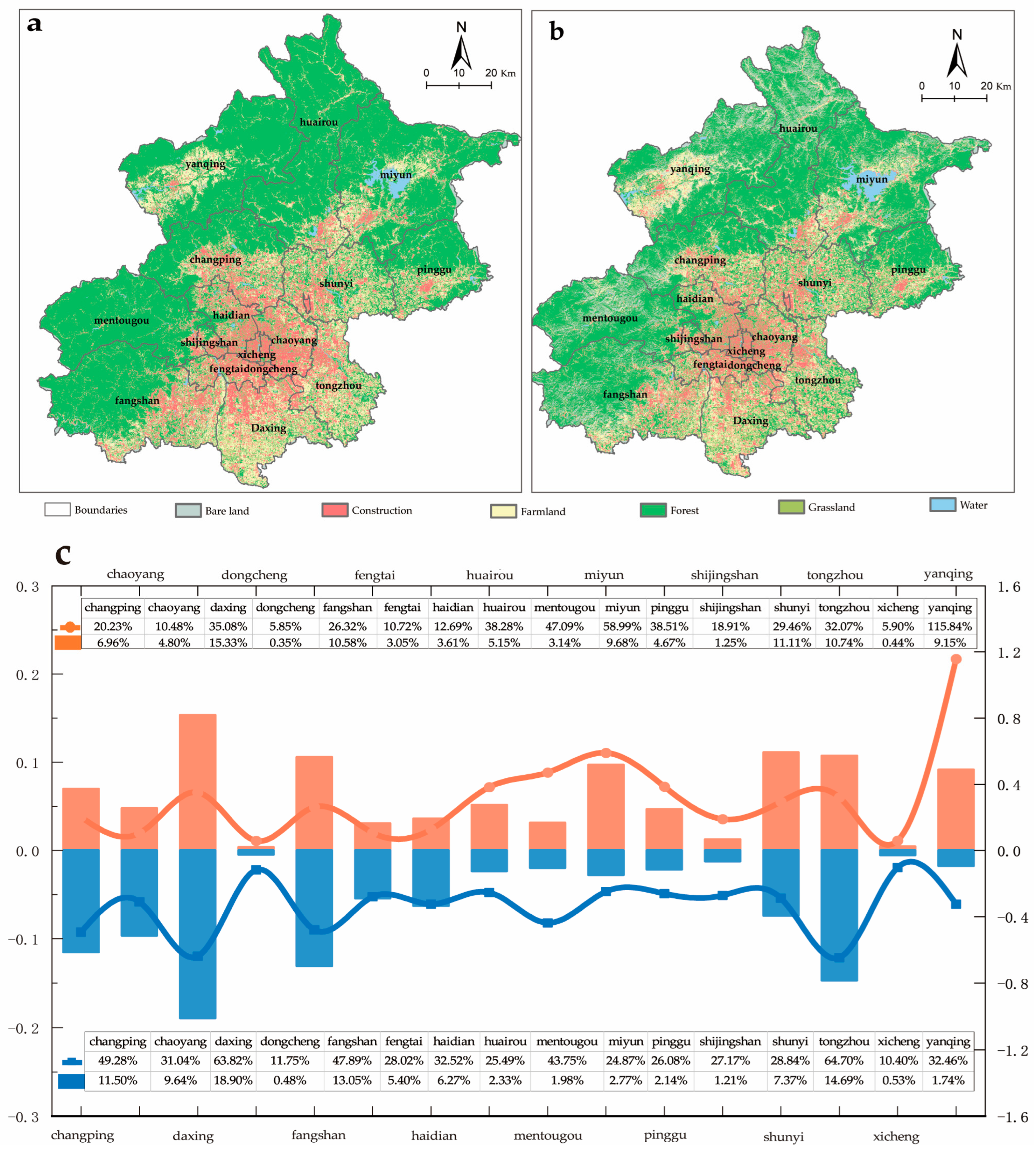
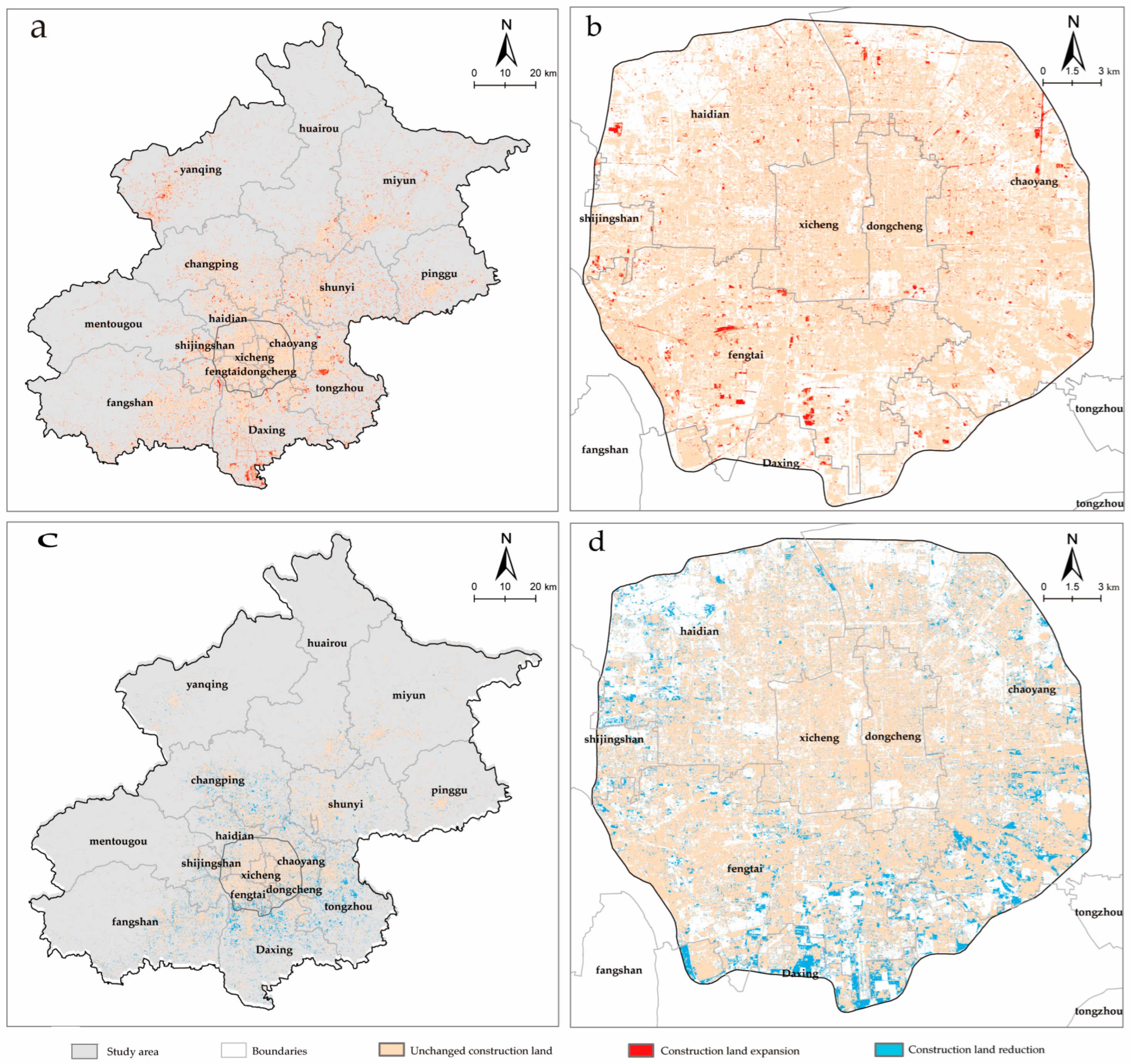
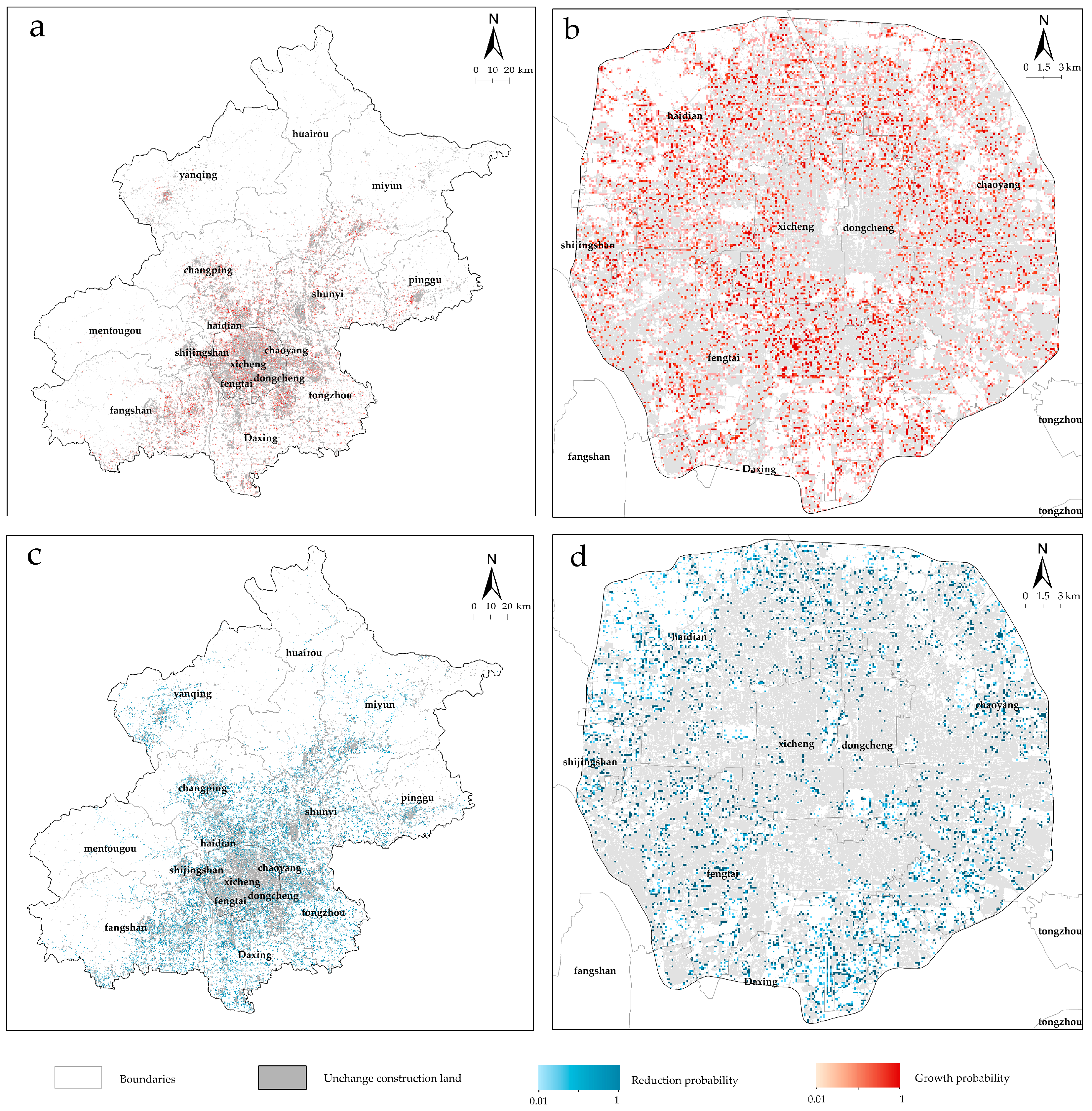
From 2016 to 2020, the district with the largest increase in construction land area in Beijing was Daxing district, accounting for 15.33% of the total increase. Next were Shunyi, Tongzhou, and Fangshan districts, accounting for 11.11%, 10.74%, and 10.58%, respectively (Figure 3). These four districts are also the areas with the largest existing construction land areas, excluding Chaoyang district. The regions with the smallest growth were Dongcheng and Xicheng districts, accounting for only 0.44% and 0.35%, respectively. Overall, the expansion of construction land in Beijing is concentrated in the southern part of the core area, where these regions typically have larger land areas and can accommodate more construction land expansion. This aligns with Beijing’s planning strategy for the southern region. We also compared the growth rates of different districts. Yanqing district, despite its smaller base, is the fastest growing region, with a growth rate of 115.84%. This may be related to Yanqing district’s recent development in ecological tourism and leisure resorts. Dongcheng district and Xicheng district remain the regions with the lowest growth rates, at 5.90% and 5.85%, respectively. This may be because these areas, as the city center, have limited expansion space and already possess relatively well-developed infrastructure and construction land layout. Overall, construction land growth in the city’s outlying suburban areas is significant, with generally high growth rates. This aligns with the recent transfer of urban center functions and industrial expansion to these regions. The growth rate in urban central areas is relatively low, with expansion exhibiting a fragmented pattern. More noticeable growth is concentrated along transportation routes and in peripheral areas such as Daxing and Fengtai (Figure 4a,b).

3.1.2. Construction Land Reduction

The districts of Daxing and Tongzhou exhibit the most significant reduction, representing 18.90% and 14.69% of the total decrease, respectively (Figure 3). Additionally, these districts demonstrate the highest decreasing rates, at 63.82% and 64.70%, in comparison to the other districts. These two districts are subject to more extensive construction land adjustments in Beijing’s urban planning, which may involve larger-scale urban renewal, industrial transformation, or ecological protection projects. The second-largest scale and rate of reduction is observed in Changping and Fangshan, at 49.28% and 47.89%, respectively. The decreasing rate in Mentougou is slightly lower than that in Fangshan (43.75%), although the original construction land area in the region is smaller, and the decreasing scale accounts for only 1.98% of the total decrease. From a spatial perspective, the reduction in construction land has been concentrated in the urban fringe areas, particularly to the south and southeast of the central urban districts, where relatively large areas have been scaled back (Figure 4c,d).

3.2. Results of Validation and Sensitivity Analysis

3.2.1. Modeling Validation

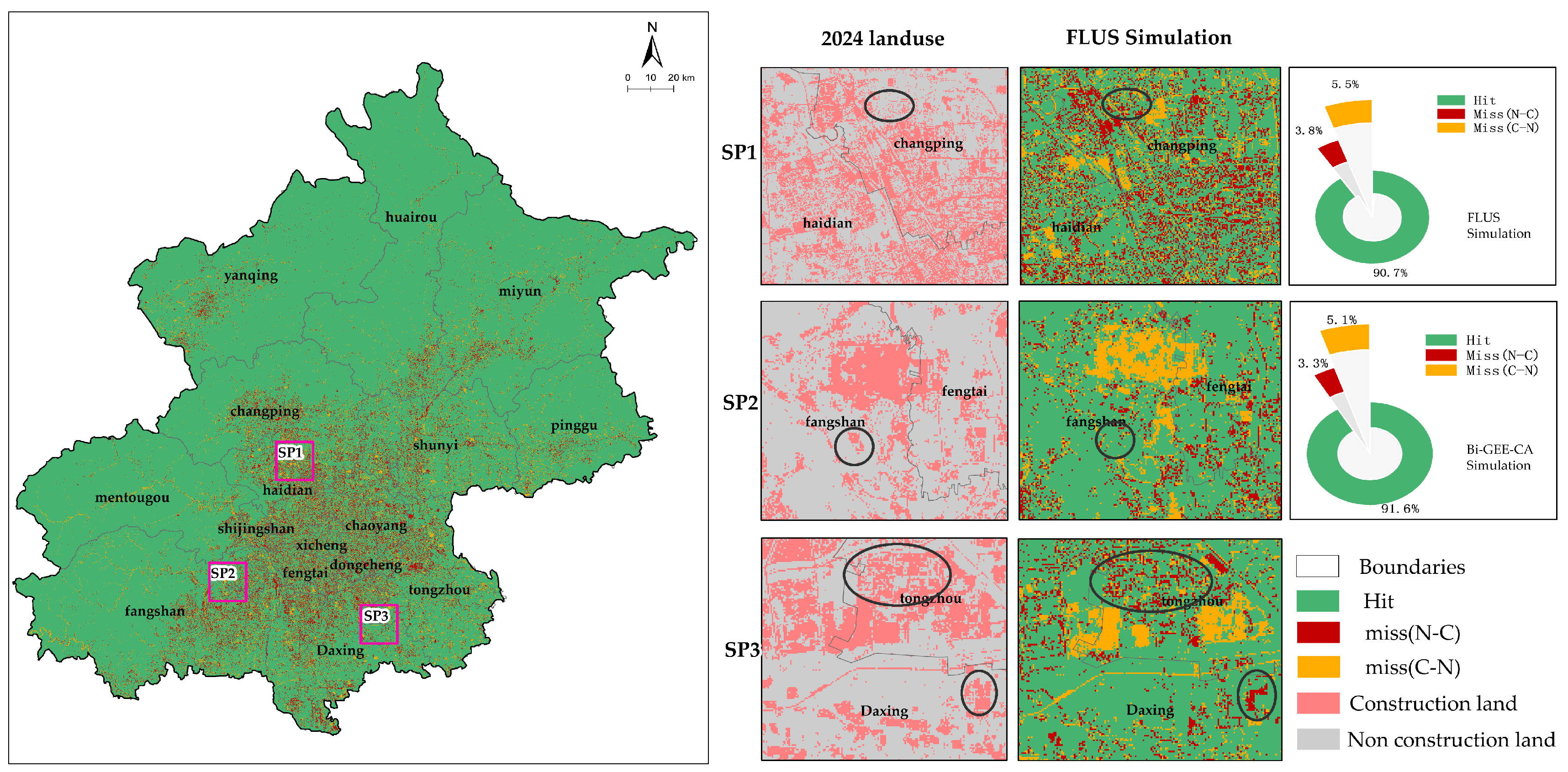
Based on the trends of urban expansion and reduction in Beijing from 2016 to 2020, this period was used as a sample (training set) to train the model. The simulated built-up land in Beijing for 2024 was then compared with the observed built-up land in the same year to validate the Bidirectional GEE-CA model. The average Kappa value was 0.67, and the average FoM value was 0.19. Figure 5 illustrates the comparison between the simulated construction land pixels and the actual construction land layout in 2024, which has been classified into three scenarios: Hit, Miss (C-N), and Miss (N-C). In Beijing, the proportion of Hit is 91.55%, while the proportions of Miss (C-N) and Miss (N-C) are 3.30% and 5.15%, respectively (Figure 5a). Within the fifth ring road, the percentage of Hit is 72.28%, while the percentage of Miss (C-N) and Miss (N-C) are 4.92% and 22.80%, respectively (Figure 5b). Statistical analyses and comparisons were also conducted for each district (Figure 5c). The deviations in the simulation primarily stem from the modeling of construction land expansion, especially in urban core areas where high urbanization and limited available space for development prevail. In these regions, new construction land tends to emerge in a dispersed manner, driven by policy-guided urban growth, which the CA model fails to fully capture. This is likely due to the model’s inability to adequately simulate leapfrog urban expansion, as noted by Zhuang et al. [57], resulting in significant discrepancies in the simulation outcomes. The model is more effective in simulating the reduction of construction land, and the error rate is not significantly different between the city-wide scale and the core area scale, which better achieves the prediction effect of the reduction of construction land.

The Sentinel-2 data used in this study is a dataset collected starting from 2015, and we selected three time points (2016, 2020, and 2024) for model validation. Specifically, data from 2016–2020 was used for model training, and data from 2020–2024 was used for model accuracy validation. This represents the best possible configuration within the limits of the available data.

3.2.2. Sensitivity Analysis

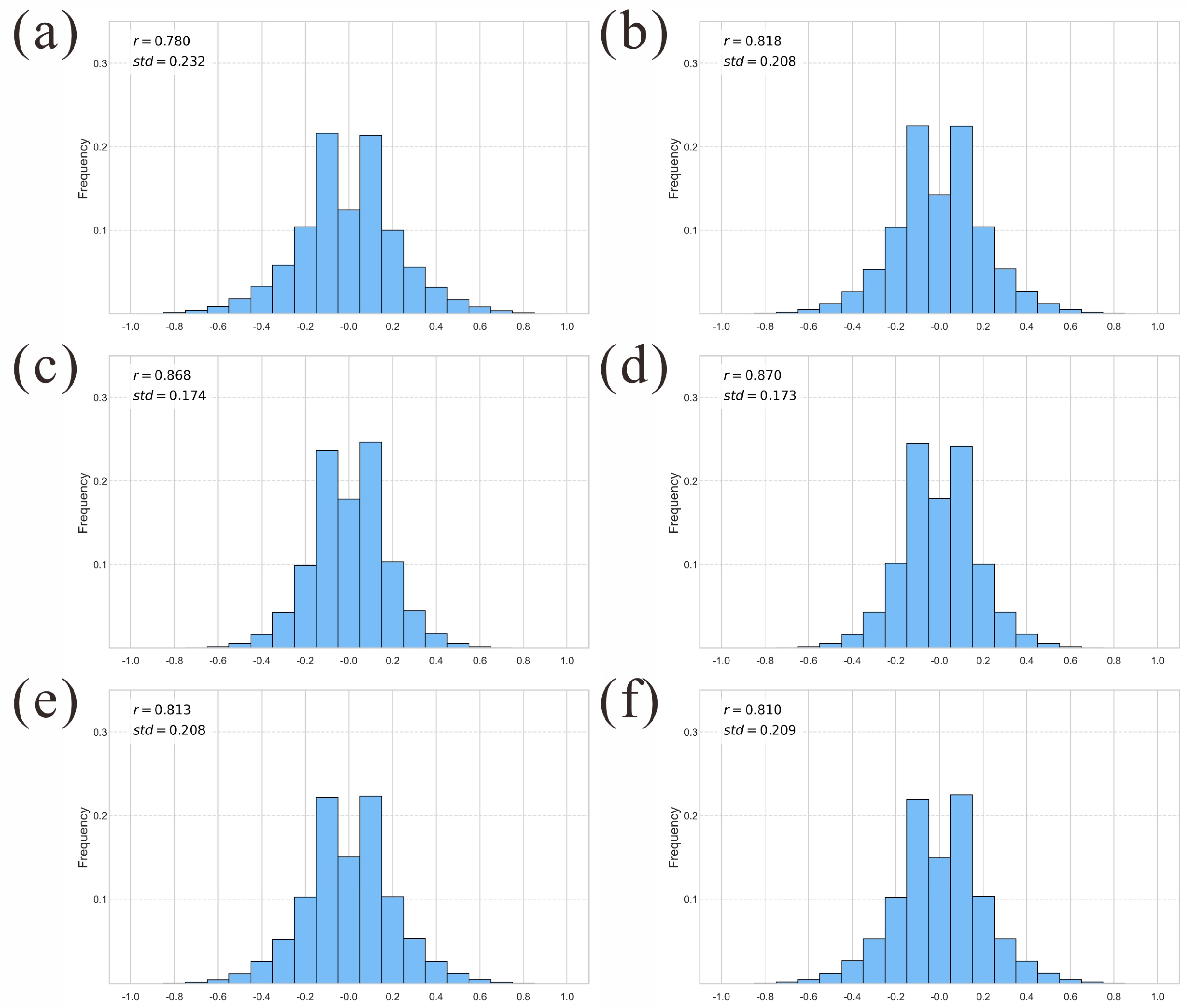
To analyze the sensitivity of parameter settings in the simulation process, we designed six additional simulation groups by modifying parameters, with each group repeated 100 times. These six sets of simulation results were then compared at the pixel scale with the 100 simulation results under baseline parameters, as shown in Figure 6. The results indicate that when the neighborhood size was adjusted to 3 × 3 and 7 × 7, the correlation coefficients with the baseline results (5 × 5) were 0.78 and 0.82, with standard deviations of 0.23 and 0.21, respectively. Additionally, 81% and 85% of the pixel values exhibited differences within the range of −0.3 to 0.3. When the iteration count was adjusted to 10 and 20, the correlation coefficients with the baseline results (15 iterations) were both 0.87, with standard deviations of 0.17 for both. Furthermore, 91% and 91% of the pixel values showed differences within the −0.27 to 0.27 range. When the number of decision trees in the random forest model was adjusted to 90 and 110, the correlation coefficients with the baseline results (100 trees) were both 0.81, with standard deviations of 0.21 for both. In these cases, 85% and 85% of the pixel values had differences within the same range.

Overall, the simulation results after parameter changes exhibit strong correlations and minor discrepancies compared to the baseline results, with the frequency distribution patterns of all six parameter groups demonstrating high similarity. Specifically, the model demonstrates differential sensitivity to parameter adjustments, with the number of iterations being the least influential factor, followed by the number of decision trees, while the neighborhood size has the most pronounced impact on simulation outcomes. The results for neighborhood size and decision trees are similar, especially when the neighborhood size is 7 × 7 (Figure 6).

3.3. Spatial Characteristics and Distribution of Construction Land Consolidation Potential

3.3.1. Future Simulation in 2035

We simulated 100 scenarios to obtain the probability distribution of land use expansion or consolidation in 2035, as shown in Figure 7. The purpose of conducting 100 repeated simulations is to account for the variability inherent in each individual simulation outcome. By aggregating the results from all 100 simulations and calculating the frequency of occurrence for each grid cell, we can identify regions that exhibit high-frequency expansion or reduction. Based on our simulated probabilities, the overall growth in construction land primarily occurs in the southern regions characterized by high density, with development occurring along transportation arteries, industrial parks, and surrounding areas of existing construction land. Suburban areas such as Changping, Daxing, and Fangshan, as well as new towns and satellite cities, also exhibit moderate expansion.

In contrast, the outlying suburban areas show a more significant reduction in construction land area, primarily consisting of scattered plots. The simulated reduction hotspots are not randomly scattered but cluster in areas with distinct socioeconomic and locational profiles, revealing the model’s capacity to capture underlying policy-driven processes. For example, model identifies the old heavy industrial bases in the near-suburban Shijingshan district as high-priority reduction zones primarily due to their characteristically low nighttime light intensity coupled with increasing relative distance to the city’s evolving economic cores. It aligns precisely with Beijing’s “Non-Capital Function Relocation” policy, where such inefficient, low-productivity clusters are targeted for transformation or redevelopment. Meanwhile, ecological conservation and land consolidation are found in far-suburban areas (e.g., Miyun, Yanqing, Huairou). The reduction potential in these districts is strongly associated with their proximity to key ecological features (e.g., water bodies, forest lands) and lower development pressure (indicated by low nighttime light). This configuration reflects a socioeconomic driver, where land use is prioritized for ecosystem service provision over intensive construction, aligning with the city’s requirements for ecological protection and agricultural land conservation.

At the core area scale, regions with a high probability of construction land growth are notably concentrated in Fengtai, Xicheng, Haidian, and Chaoyang districts. Regions with a high probability of reduction are more dispersed and primarily located at the edges of the core area. Based on simulation results, the reduction in construction land will still be guided by layout optimization, with the core focus on adjusting low-efficiency land use and protecting green spaces.

3.3.2. Spatial Autocorrelation Analysis of Potential Areas

To enhance the spatial analytical depth of this study, a spatial autocorrelation analysis was conducted to assess spatial dependence and clustering of construction land consolidation potential. This analysis is crucial for understanding geographical patterns and validating the robustness of the predictive model. Specifically, we employed two widely used spatial statistics: Moran’s I and Local Indicators of Spatial Association (LISA). For expansion potential areas, the Moran’s I value of 0.1890 indicates weak positive spatial autocorrelation, suggesting that regions with higher expansion potential are spatially clustered with other high-potential areas. This clustering is statistically significant, as demonstrated by a p-value of 0.001, which is well below the 0.05 significance threshold. The Z-score of 48.1484 further supports the significance of the positive autocorrelation. Similarly, for reduction potential areas, the Moran’s I value of 0.1755 reveals weak positive spatial autocorrelation, indicating that regions with higher reduction potential also exhibit spatial clustering. This result is statistically significant, with a p-value of 0.001, confirming that the observed spatial clustering is unlikely to occur by chance. The Z-score of 40.1440 further validates this finding. The global Moran’s I result indicates statistically significant positive spatial autocorrelation, suggesting that both types of potential areas exhibit distinct spatial clustering patterns. These findings imply that the model’s predictions align with underlying geographical trends.

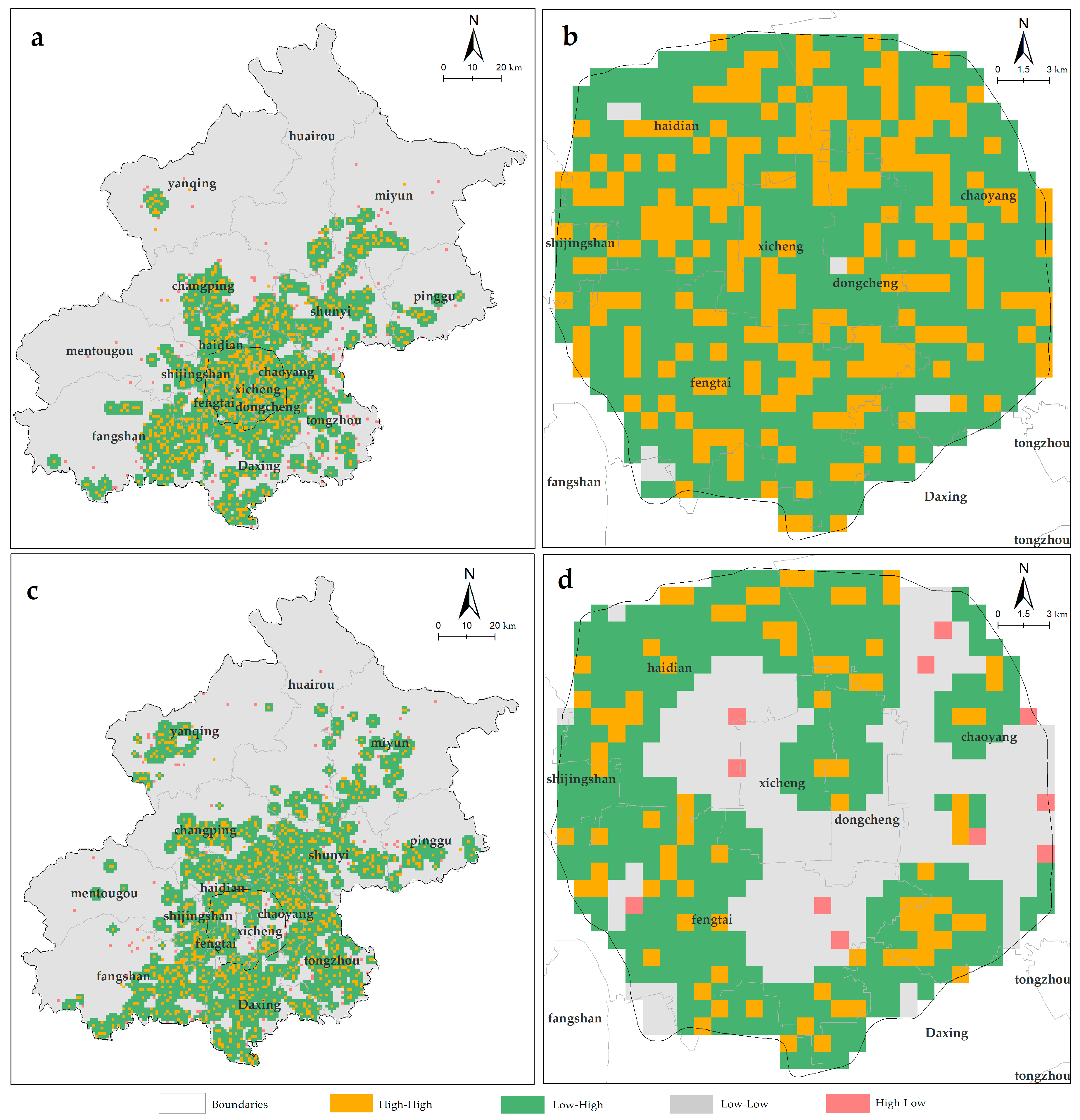
LISA analysis reveals the spatial distribution of clustering or dispersion, providing a more granular understanding of regional spatial patterns. For visualization, LISA results effectively depict the clustering distribution of potential areas within the study region, enabling the precise identification of key geographic areas for intervention. As shown in Figure 8, LISA analysis identifies significant spatial clustering for both expansion potential and reduction potential. For expansion potential, High–High (6.20%) and Low–High (21.83%) clusters are predominantly found in core urban areas, indicating that expansion potential is geographically concentrated in regions with existing infrastructure and development capacity. The Low–Low cluster (71.18%) is primarily located on the urban periphery and in areas with lower development potential. These regions generally exhibit weaker economic and infrastructure conditions, suggesting limited suitability for further expansion. The High–Low cluster (0.79%) is sparsely distributed. For reduction potential, distinct spatial clustering is also observed. High–High (6.37%) and Low–High (28.61%) clusters are mainly located in environmentally sensitive or underdeveloped areas requiring protection or mitigation. These clusters are predominantly found on the outskirts of core urban areas, suggesting that land use in these zones should prioritize ecological protection, environmental restoration, or reduced development intensity. The Low–Low cluster (64.42%), which is more widespread, presents less urgency for land-use restrictions and reduction interventions. Overall, the analysis indicates that land reclamation efforts should prioritize High–High and Low–High clusters. The High–High clusters, characterized by significant clustering, represent areas with substantial intervention potential and should be prioritized for land consolidation. Conversely, areas with Low–High distribution, exhibiting considerable variability in potential, are more heterogeneous and require targeted interventions to address and optimize potential disparities.

3.3.3. Distribution of Construction Land Consolidation Potential

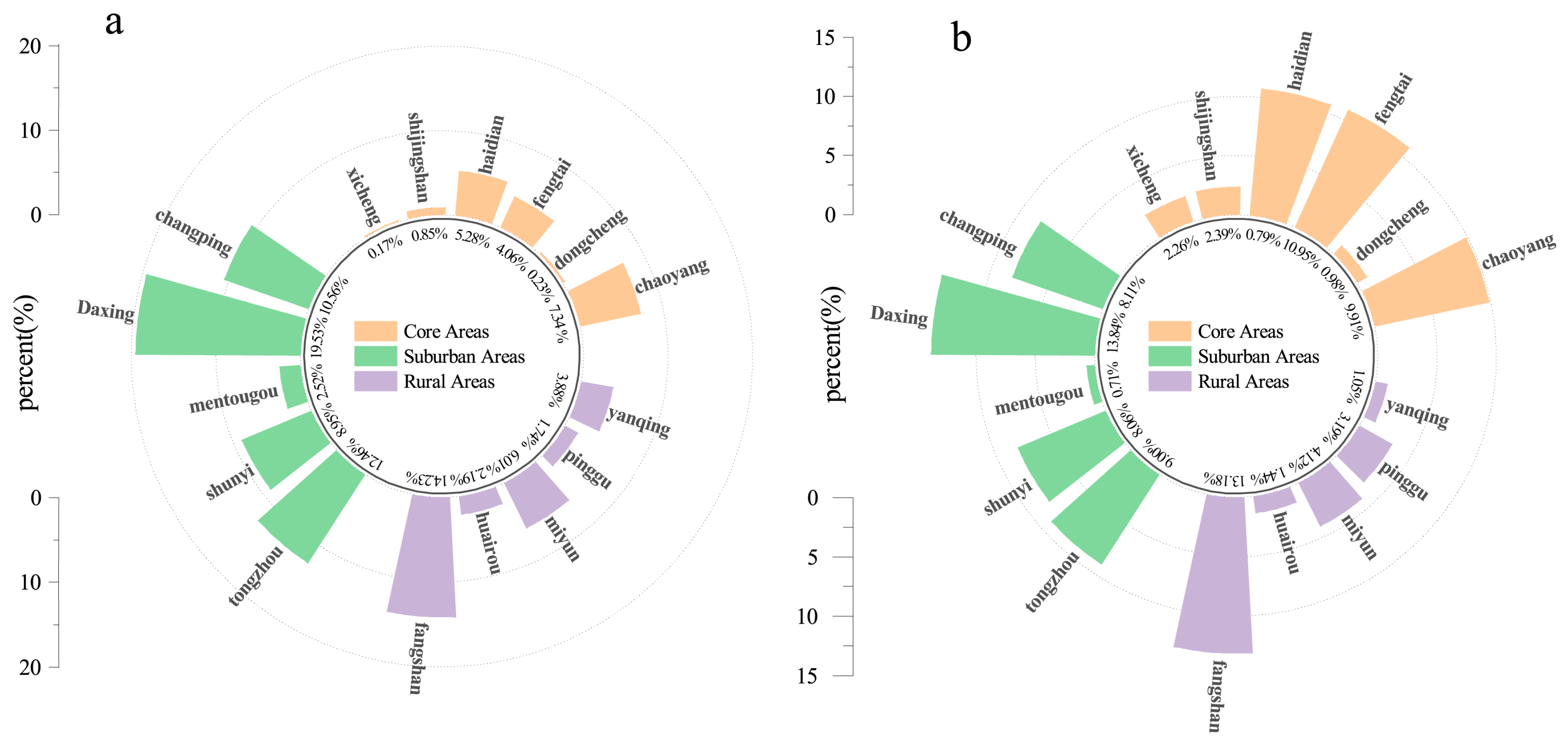
The Natural Breaks Method was used to classify the probabilities of construction land consolidation potential into three levels. Grids with a probability greater than 0.65 were classified as high probability areas, accounting for approximately 22.03% of the total grids. The medium probability area, ranging from 0.25 to 0.65, accounted for 21.60%, while the low probability area (below 0.25) accounted for 56.37%. The distribution of areas with high consolidation potential was statistically analyzed, as shown in Figure 9. It was found that the potential areas for future construction land consolidation were mainly concentrated in Daxing, Fangshan, and Tongzhou, accounting for 46.21% of the total scale. The Urban Core Area, represented by Dongcheng and Xicheng districts, had the lowest consolidation potential, accounting for only 0.40% of the total scale. Specifically, as Beijing’s Core Functional Area for Political, Cultural and International Exchange, the core area will maintain a certain level of urban function and population density in the future, and the reduction in this area will be relatively small.

In the future, while maintaining certain urban functions, Chaoyang, Haidian, and Fengtai districts will focus on urban renewal and industrial upgrading to meet the needs of urban development. Therefore, a moderate reduction in construction land is expected. Daxing, Shunyi, and Tongzhou districts, along with other Outer Suburban districts, are projected to experience relatively larger reductions in the future. In their future development, these areas will place greater emphasis on optimizing the industrial structure and spatial development layout, reducing construction land to create space for future development. Mentougou, Fangshan, and parts of the mountainous areas of Changping, Huairou, Miyun, and Yanqing districts serve as important ecological barriers for the city. In the future, construction land will need to be drastically reduced to protect the ecological environment and natural landscape, and to ensure coordinated development of ecology and economy.

4. Discussion

4.1. Comparative Analysis of Models

4.1.1. Model Comparability

The FoM and Kappa coefficient are widely recognized indicators for validating land-use simulation accuracy, enabling quantitative comparison between simulated and observed patterns [46,56,58]. These indicators have been systematically applied to evaluate mainstream models including FLUS [56,59,60], SLEUTH [58], ST-CA [61], PLUS [62], and Logistic-CA [63] (Table 3).

FoM specifically quantifies predictive capability through spatial consistency analysis of land-change classifications, with values spanning 0–1 (higher indicating greater accuracy). Benchmark studies report typical FoM ranges of 0.1–0.3 (Table 3), positioning our bidirectional GEE-CA model’s FoM (0.19) as competitively robust relative to existing literature. This indicates that our model’s performance is accepted with the field’s standards.

Conversely, Kappa coefficient variability across studies is pronounced. For instance, Meng et al. [46] reported a Kappa coefficient range of 0.65–0.95 across various cities, Saxena and Jat [58] observed a range of 0.4–0.55, and Wang et al. [63] found a range of 0.45–0.47. Following Landis and Koch [64], our Kappa value of 0.68 denotes substantial agreement (0.6–0.8 range) between simulations and observations. While we acknowledge the inherent limitations of such cross-study comparisons due to differences in study areas and data sources, this analysis provides valuable evidence that our model produces spatially plausible results that are comparable to those of established models in the field.

Table 3. Accuracy validation results of other land use models in previous studies.

Authors	Model	Level	FoM	Kappa Coefficient
Meng et al. [46]	GEE-CA	City	0.14–0.31	0.65–0.95
Liu et al. [56]	FLUS	Regional	0.12	0.79
Saxena and Jat [58]	SLEUTH	City	0.11–0.3	0.4–0.55
Geng et al. [61]	ST-CA	National	0.18	0.99
Wang et al. [63]	Logistic-CA	City	0.20–0.21	0.45–0.47
Chen et al. [65]	FLUS	Regional	0.12–0.36	-
Zhang et al. [66]	PLUS	City	0.146	0.772
Li et al. [67]	FLUS	Regional	0.10–0.29	-
This study	Bidirectional GEE-CA	City	0.19	0.68

Note: FLUS: future land use simulation model; SLEUTH: slope-land use-exclusion-urban extent-transportation-hill shade model; ST-CA: spatiotemporal convolution-based cellular automata model; PLUS: patch-generating land use simulation model.

Table 3. Accuracy validation results of other land use models in previous studies.

Authors	Model	Level	FoM	Kappa Coefficient
Meng et al. [46]	GEE-CA	City	0.14–0.31	0.65–0.95
Liu et al. [56]	FLUS	Regional	0.12	0.79
Saxena and Jat [58]	SLEUTH	City	0.11–0.3	0.4–0.55
Geng et al. [61]	ST-CA	National	0.18	0.99
Wang et al. [63]	Logistic-CA	City	0.20–0.21	0.45–0.47
Chen et al. [65]	FLUS	Regional	0.12–0.36	-
Zhang et al. [66]	PLUS	City	0.146	0.772
Li et al. [67]	FLUS	Regional	0.10–0.29	-
This study	Bidirectional GEE-CA	City	0.19	0.68

Note: FLUS: future land use simulation model; SLEUTH: slope-land use-exclusion-urban extent-transportation-hill shade model; ST-CA: spatiotemporal convolution-based cellular automata model; PLUS: patch-generating land use simulation model.

4.1.2. Model Reliability

The aforementioned comparative results merely indicate the predictive competency of our model, without evidencing its superiority within the context of reduction planning. To address this, we selected FLUS model [56]—which has been empirically demonstrated to outperform established models (e.g., ANN-CA, CLUE-S, and Logistic-CA) while incorporating projected construction land reduction in Beijing—for benchmarking against our model outputs. Both the bidirectional GEE-CA and FLUS models simulated 2020–2024 construction land changes. The FLUS model captures urban expansion patterns (Figure 10), whereas the bidirectional GEE-CA model concurrently simulates both expansion and reduction dynamics. This capability stems from its dedicated land reduction module and dynamic modeling of reduction planning constraints. Notably, the FLUS model requires total construction land change inputs without independent control of expansion/reduction quantities.

Quantitative assessment was performed using the Figure of Merit (FoM) metric, recognized for superior sensitivity to spatial consistency in land-change simulations [46,56]. The FoM indicator of bidirectional GEE-CA model (0.19) outperforms the value of FLUS model (0.07), which indicates a significant improvement in simulating complex scenarios where expansion and reduction coexist. We further calculated Hit, Miss (N-C), and Miss (C-N) by comparing simulation of FLUS and the actual construction land in 2024. In Beijing, the proportions of Hit, Miss (N-C), and Miss (C-N) are 90.73%, 3.82%, and 5.45%. These results show that the Hits of FLUS are lower than those of bidirectional GEE-CA model (Figure 10). It can be observed that bidirectional GEE-CA model’s enhanced precision in simulating construction land dynamics.

4.1.3. Inheritance and Development of Models

Indeed, the bidirectional GEE-CA model developed in this study inherits and builds upon the GEE-CA model by Meng et al. [46] and the FLUS model by Liu et al. [56], demonstrating a clear lineage of development. Our bidirectional GEE-CA model has been enhanced in terms of driving factors, transition restrictions, and CA transition rules. Table 4 summarizes the connections and differences between our model and other models.

In terms of driving factors, all existing studies have incorporated elevation variables (e.g., DEM, slope data), and most have also included proximity variables (e.g., distance to roads, city centers). This study adopts the same two categories of variables. The most significant adjustment in variable selection is the introduction of nighttime light data, as suggested by Chen et al. [65]. Nighttime light data can serve as an important indicator for measuring urban development efficiency, reflecting spatial heterogeneity within cities. It also helps to identify inefficient land use and provides guidance for construction land reduction.

Regarding transition restrictions, this study offers a more comprehensive consideration. Zhang et al. [66] and Li et al. [67] incorporated policy-defined expansion boundaries to constrain urban growth, while Meng et al. [46] treated water bodies as restrictive factors. Since our model simulates both expansion and reduction of construction land, in addition to commonly used water constraints, we also integrate policy zones from the Beijing Master Plan—such as permitted, restricted, and prohibited construction areas—and further introduce roads as a restrictive factor in the reduction module. Compared to previous studies, our approach pays greater attention to urban internal details and policy guidance.

Finally, in terms of cellular automata transition rules, prior research has predominantly focused on urban expansion, lacking the ability to explain or predict policy-driven reduction. The key innovation of this study lies in establishing a bidirectional transition mechanism that simultaneously simulates both expansion and reduction, representing a major advancement over existing models. This enhancement better addresses the current demand for construction land reduction in certain megacities. Compared to the FLUS model, our bidirectional approach offers a more comprehensive solution for managing urban land use dynamics.

Table 4. The consistency and differences of driving factors, transition restrictions, and transition rules between this study and relative CA-based research.

Authors	Driving Factors of Construction Land Changes			Transition Restrictions			CA Transition Rules
	Elevation Variables	Proximity Variables	Nighttime Light	Water	Road	Policy	Construction Land Expansion	Construction Land Reduction
Meng et al. [46]	√	√	×	√	×	×	√	×
Liu et al. [56]	√	×	×	×	×	×	√	×
Chen et al. [65]	√	√	√	×	×	×	√	×
Zhang et al. [66]	√	√	×	×	×	√	√	×
Li et al. [67]	√	×	×	×	×	√	√	×
This study	√	√	√	√	√	√	√	√

Note: √ represents that this variable/restriction/rule was used in the corresponding study, × indicates that this variable/restriction/rule was not used in the corresponding study.

Table 4. The consistency and differences of driving factors, transition restrictions, and transition rules between this study and relative CA-based research.

Authors	Driving Factors of Construction Land Changes			Transition Restrictions			CA Transition Rules
	Elevation Variables	Proximity Variables	Nighttime Light	Water	Road	Policy	Construction Land Expansion	Construction Land Reduction
Meng et al. [46]	√	√	×	√	×	×	√	×
Liu et al. [56]	√	×	×	×	×	×	√	×
Chen et al. [65]	√	√	√	×	×	×	√	×
Zhang et al. [66]	√	√	×	×	×	√	√	×
Li et al. [67]	√	×	×	×	×	√	√	×
This study	√	√	√	√	√	√	√	√

Note: √ represents that this variable/restriction/rule was used in the corresponding study, × indicates that this variable/restriction/rule was not used in the corresponding study.

4.2. Types of Construction Land Consolidation

Based on the potential for expansion and consolidation across various areas of Beijing, and considering their functional roles and rectification strategies, the 16 regions have been classified into three categories: Optimization Type, Enhancement Type, and Conservation Type (

Table 5. Characteristics and representative districts of different types of consolidation.

Type	Core Objective	Characteristics	Typical Measures	Representative Districts
Enhancement Type	Enhancing Industrial Competitiveness and Urban Functions	Significant trends of expansion and reduction	Industrial Upgrading, land consolidation, and optimization of public services	Chaoyang, Haidian, Tongzhou, Daxing, Shunyi
Optimization Type	Decentralizing Non-core Functions and Improving Spatial Quality	Maintain low-level expansion and reduction	Relocation of low-end industries, removal of illegal constructions, and preservation of historical features	Dongcheng, Xicheng, Shijingshan
Conservation Type	Prioritizing Ecology and Promoting Sustainable Development	Minor reduction, with a relatively low proportion of expansion	Protecting agricultural and ecological resources and regulating tourism development	Mentougou, Miyun, Yanqing

). Optimization Type areas aimed at improving existing functions, Enhancement Type areas are concerned with the promotion of urbanization through large-scale development and upgrading, while Conservation Type areas prioritize the preservation of the ecological environment.

The primary function of the Optimization Type is the mitigation of non-capital functions and the adjustment of spatial layouts. The areas earmarked for renovation encompass Dongcheng, Xicheng, Shijingshan, and other regions that boast convenient transportation connections and relatively mature land conditions. These areas are typically distinguished by high building density and well-developed public services and infrastructure, although their potential for expansion is somewhat constrained. Consequently, the trends of expansion and consolidation in these regions are relatively modest. The primary objective of optimization efforts is the reallocation of resources to alleviate pressures from low-end industries and the population. The primary objective is to enhance the efficiency of existing resource utilization, optimize functional layouts, and improve both land use efficiency and the overall quality of regional functions, thereby achieving comprehensive improvements in functionality.

The Enhancement Type, which is designed to strengthen functional structures and enhance industrial competitiveness, is primarily implemented in suburban and outer suburban areas of the city, including Fangshan, Chaoyang, Daxing, Fengtai, Haidian, Shunyi, Changping, and Tongzhou. These areas are of significance in the context of urban development, as they demonstrate notable patterns of both expansion and consolidation. The functional roles of these areas are diverse, encompassing commercial, residential, industrial, and other uses. The primary objective of the renovation initiative is to substantially enhance the quality of regional functions through large-scale land development and industrial guidance. These areas are undergoing a gradual transformation into comprehensive functional zones, thus becoming critical components of the urbanization process.

The designated Conservation Type, encompassing Huairou, Mentougou, Miyun, Pinggu and Yanqing, is a region of particular ecological significance, with a focus on the conservation of land. These regions are distinguished by their favorable natural environments, abundant ecological resources, and scenic value. Furthermore, they provide support for functions related to tourism and recreation. The development of these areas is subject to stringent environmental protection regulations and strict land-use restrictions. The scope of expansion is relatively constrained, and in certain instances, the scale of development is deliberately diminished. The objective of development in Conservation Type areas is not expansive growth but rather the preservation of regional natural landscape features and the sustainable use of natural resources. In the context of land consolidation initiatives within these regions, the primary focus is on ecological restoration and the enhancement of the ecological environment. This objective is pursued through the implementation of stringent protection measures and the reduction of superfluous development activities. These efforts include the reduction of illegal mining, the rational planning of tourism development, and the minimization of ecological damage caused by substandard construction.

4.3. The Applicability of the Model

Theoretically, the proposed bidirectional GEE-CA model advances conventional land-use simulation frameworks by integrating dual-process mechanisms for both construction land expansion and reduction. Traditional approaches [46,56] predominantly focus on unidirectional urban expansion—modeling non-urban to urban land conversion under global urbanization trends. These models inherently assume prohibitively high reversion costs and minimal probability for construction-to-non-construction land transitions. However, as megacities increasingly approach developmental ceilings, the feasibility of construction land reversion (e.g., industrial site retirement, ecological restoration) becomes non-negligible [68]. Consequently, urban expansion-oriented simulation paradigms exhibit fundamental limitations in addressing contemporary spatial governance challenges.

A new model is developed to overcome conventional limitations through its spatial expansion-reduction coupler. First, it integrates reduction drivers and expansion demand parameters into a unified computational framework. Second, a bidirectional feedback mechanism establishes dynamic constraints between consolidation volume and new construction volume, adhering to planning-permitted land replacement ratios. Ultimately, this enables precise quantification of critical reduction processes—including industrial zone retirement timelines and efficiency of illegal-structure demolition to afforestation conversion. Fundamentally resolving the cognitive blind spot wherein traditional tools “see only expansion, ignore reduction” in territorial consolidation, the framework provides full-cycle simulation support for urban land consolidation.

Practically, the model demonstrates strategic applicability in China’s coastal megacities—exemplified by Shanghai, Jiangsu, and Guangdong—where accelerated development and advanced economic thresholds necessitate context-sensitive construction land reduction. Our framework delivers scientifically grounded solutions through its visualization and simulation capabilities, optimizing urban–rural spatial configurations while adapting reduction parameters to regional specificities (e.g., industrial restructuring in the Pearl River Delta). Future applications of this model will transform land consolidation policies from static quota allocation into a quantifiable, early-warning-enabled, and iteratively optimizable dynamic implementation system. This advancement elevates territorial planning supervision precision, fundamentally resolving the governance predicament where plans remain ornamental while implementation crawls.

Furthermore, this model demonstrates three core values in international applications, with explicit adaptations to address diverse planning systems and data availability constraints: In developed economies characterized by mature regulatory frameworks and high-resolution spatial data infrastructure, it facilitates post-industrial landscape regeneration through spatial restructuring, converting abandoned industrial lands into ecological zones to enhance ecosystem service value. Documented implementations include industrial wastelands in the U.S. Rust Belt [69] and brownfield revitalization in Germany’s Ruhr region, utilizing brownfield revitalization with comprehensive geospatial databases [70]. Secondly, in rapidly urbanizing emerging economies, where governance structures are often fragmented and spatial data availability is limited, the model employs a socio-economic dual-dimensional assessment framework adaptable to participatory mapping and medium-resolution satellite imagery, enabling context-sensitive informal settlement upgrading in Indian and Brazilian communities through integrated community-driven data collection [71]. Thirdly, in extreme disturbance zones requiring rapid response, the model supports scalable damage evaluation protocols adjustable to varying data quality—from satellite-based damage interpretation in Ukraine’s post-conflict reconstruction [72] to real-time sensor-integrated resilience mechanisms in Japan’s earthquake/tsunami-affected regions, ensuring alignment with dynamic monitoring needs [73]. These tailored implementation pathways underscore the model’s flexibility across differing institutional arrangements and technical conditions, substantiating its global applicability by explicitly addressing planning paradigms and data environments.

Additionally, our modeling demonstrates substantial promise for advancing climate adaptation and mitigation strategies by enabling dynamic land-use simulations under varying environmental pressures. For climate adaptation, the framework can simulate responses to extreme weather events—such as flooding or sea-level rise—by identifying vulnerable built-up areas and optimizing resilient spatial layouts. In mitigation contexts, the model quantifies carbon sequestration potential through land-cover transitions, supporting nature-based solutions like afforestation or wetland restoration to enhance ecosystem carbon sinks, which aligns with research on forest carbon flux responses to climate variability. By integrating climate projection data, future iterations could further refine decision-support tools for regional climate action plans, addressing urgent gaps in sustainable spatial planning.

4.4. Limitations and Further Improvement

This study acknowledges limitations requiring attention within land consolidation frameworks. The present bidirectional CA model is specifically optimized for simulating the critical interplay between construction land and non-construction land, which is the central process mandated by urban reduction planning policies. While transitions within non-construction land categories (e.g., farmland to wetland) are ecologically significant [56], they fall outside the immediate operational focus of this planning instrument. This focused design provides a robust foundation for addressing reduction planning. The core logic of our framework can be extended in future work to incorporate multi-class transition matrices for broader land system simulation. This enhancement will allow the model to simulate a fuller range of land-use interactions, making it applicable to integrated land consolidation and ecological conservation planning beyond the specific scope of reduction planning.

Second, the proxy variables employed (e.g., nighttime light, accessibility) effectively capture macro-scale socioeconomic dynamics to ensure the model’s transferability across cities, though they may not resolve finer-grained mechanisms like specific factory closures. Future work will thus pursue a dual path: integrating high-resolution data (e.g., firm-level, mobility metrics) for mechanistic depth in data-rich settings while further refining the current proxy-based framework to balance interpretive power, accuracy, and cross-city applicability for broader policy screening.

Third, while the model provides data interfaces for regions with existing land consolidation plans, it currently lacks a scientifically robust methodology to determine appropriate reduction targets for areas initiating new consolidation initiatives. Addressing this gap requires developing predictive protocols that synthesize historical consolidation patterns, urban decay trajectories, and socioeconomic carrying capacity thresholds to establish context-specific reduction benchmarks for emerging land consolidation projects.

Fourth, while our Bidirectional GEE-CA model demonstrates robust performance in data-rich environments like Beijing, its broader applicability faces constraints related to data availability across both space and time. Spatially, performance may be constrained in regions with poor satellite data coverage, affecting classification and simulation accuracy. Temporally, the validation of long-term forecasting strength is limited by the relatively short archive of high-resolution data (e.g., Sentinel-2 from 2015). Crucially, the model’s reliance on stable, fundamental drivers (e.g., topography, water) rather than transient local variables provides a robust foundation for projection beyond the calibration period. To address these concerns and enhance model generalizability, future work should validate its performance across cities with varying socioeconomic contexts and scales—such as Shanghai (a megacity with distinct urban patterns) and mid-sized towns (with different development dynamics)—and explore integrating longer-term medium-resolution archives (e.g., Landsat) for decadal-scale analysis, alongside alternative data sources like aerial photography or multi-sensor fusion to improve resilience under diverse data conditions.

5. Conclusions

This study addresses a critical challenge in urban land consolidation: the difficulty of clearly defining the spatial location for the reduction of construction land. The proposed policy-informed bidirectional cellular automata (CA) framework for reduction planning implementation serves as a geospatial tool to quantify potential consolidation and simulate future construction land dynamics under reduction planning. This methodological extension uniquely integrates high-resolution (30 m) simulations of both construction land expansion and reduction, thereby overcoming the limitations of traditional unidirectional models such as the Future Land Use Simulation (FLUS) system. The model was validated, demonstrating better accuracy and significant improvements in precision. The application of this model to Beijing resulted in the identification of key hotspots for land consolidation and the prediction of the spatial distribution of land transformation zones through neighborhood-scale probability distributions. The results of the study indicate priority areas for consolidation and provide detailed insights into land-use trends, including areas of both expansion and reduction.

Beyond technical innovation, this framework offers transformative policy utility. It shifts land consolidation from static quota allocation towards a dynamic, simulatable, and optimizable implementation system. For planners in megacities like Beijing or Shanghai, it enables precise identification of inefficient land (e.g., outdated industrial clusters), optimizes the spatial balance between new development and ecological restoration, and provides a “policy testing ground” for achieving net reduction targets. Moreover, the model’s design, based on widely available data (e.g., nighttime light, topography), ensures strong transferability. Its core logic—managing the dual dynamics of growth and shrinkage—is relevant to diverse global contexts, facilitating post-industrial regeneration in developed economies (e.g., brownfield redevelopment), guiding informed settlement upgrading in rapidly urbanizing regions with limited data, and supporting resilience planning in areas facing climatic or conflict-related disturbances.

References

1. Zhou, Y.; Li, X.; Asrar, G.R.; Smith, S.J.; Imhoff, M. A global record of annual urban dynamics (1992–2013) from nighttime lights. Remote Sens. Environ. 2018, 219, 206–220. [Google Scholar] [CrossRef]
2. de Groot, R. Function-analysis and valuation as a tool to assess land use conflicts in planning for sustainable, multi-functional landscapes. Landsc. Urban Plan. 2006, 75, 175–186. [Google Scholar] [CrossRef]
3. Liu, Y.; Fan, P.; Yue, W.; Song, Y. Impacts of land finance on urban sprawl in China: The case of Chongqing. Land Use Policy 2018, 72, 420–432. [Google Scholar] [CrossRef]
4. Salvati, L.; Zambon, I.; Chelli, F.M.; Serra, P. Do spatial patterns of urbanization and land consumption reflect different socioeconomic contexts in Europe? Sci. Total Environ. 2018, 625, 722–730. [Google Scholar] [CrossRef] [PubMed]
5. Bagheri, B.; Tousi, S.N. An explanation of urban sprawl phenomenon in Shiraz Metropolitan Area (SMA). Cities 2018, 73, 71–90. [Google Scholar] [CrossRef]
6. Liu, Y.; Li, J.; Yang, Y. Strategic adjustment of land use policy under the economic transformation. Land Use Policy 2018, 74, 5–14. [Google Scholar] [CrossRef]
7. Oueslati, W.; Alvanides, S.; Garrod, G. Determinants of Urban Sprawl in European Cities. SSRN Electron. J. 2015, 52, 1594–1614. [Google Scholar] [CrossRef] [PubMed]
8. Chen, Y.; Chen, Z.; Xu, G.; Tian, Z. Built-up land efficiency in urban China: Insights from the General Land Use Plan (2006–2020). Habitat Int. 2016, 51, 31–38. [Google Scholar] [CrossRef]
9. Seto, K.C.; Guneralp, B.; Hutyra, L.R. Global forecasts of urban expansion to 2030 and direct impacts on biodiversity and carbon pools. Proc. Natl. Acad. Sci. USA 2012, 109, 16083–16088. [Google Scholar] [CrossRef]
10. Jiang, L.; Deng, X.; Seto, K.C. The impact of urban expansion on agricultural land use intensity in China. Land Use Policy 2013, 35, 33–39. [Google Scholar] [CrossRef]
11. Liu, X.; Ming, Y.; Liu, Y.; Yue, W.; Han, G. Influences of landform and urban form factors on urban heat island: Comparative case study between Chengdu and Chongqing. Sci. Total Environ. 2022, 820, 153395. [Google Scholar] [CrossRef]
12. Liu, X.; Zhou, Y.; Yue, W.; Li, X.; Liu, Y.; Lu, D. Spatiotemporal patterns of summer urban heat island in Beijing, China using an improved land surface temperature. J. Clean. Prod. 2020, 257, 120529. [Google Scholar] [CrossRef]
13. Nor, A.N.M.; Corstanje, R.; Harris, J.A.; Brewer, T. Impact of rapid urban expansion on green space structure. Ecol. Indic. 2017, 81, 274–284. [Google Scholar] [CrossRef]
14. Amponsah, O.; Blija, D.K.; Ayambire, R.A.; Takyi, S.A.; Mensah, H.; Braimah, I. Global urban sprawl containment strategies and their implications for rapidly urbanising cities in Ghana. Land Use Policy 2022, 114, 105979. [Google Scholar] [CrossRef]
15. Haaland, C.; van den Bosch, C.K. Challenges and strategies for urban green-space planning in cities undergoing densification: A review. Urban For. Urban Green. 2015, 14, 760–771. [Google Scholar] [CrossRef]
16. Habibi, S.; Asadi, N. Causes, Results and Methods of Controlling Urban Sprawl. Procedia Eng. 2011, 21, 133–141. [Google Scholar] [CrossRef]
17. Liang, X.; Liu, X.; Li, X.; Chen, Y.; Tian, H.; Yao, Y. Delineating multi-scenario urban growth boundaries with a CA-based FLUS model and morphological method. Landsc. Urban Plan. 2018, 177, 47–63. [Google Scholar] [CrossRef]
18. Tayyebi, A.; Perry, P.C.; Tayyebi, A.H. Predicting the expansion of an urban boundary using spatial logistic regression and hybrid raster–vector routines with remote sensing and GIS. Int. J. Geogr. Inf. Sci. 2013, 28, 639–659. [Google Scholar] [CrossRef]
19. Song, Y.; Knaap, G.J. Measuring Urban Form: Is Portland Winning the War on Sprawl? J. Am. Plan. Assoc. 2004, 70, 210–225. [Google Scholar] [CrossRef]
20. Gennaio, M.P.; Hersperger, A.M.; Bürgi, M. Containing urban sprawl—Evaluating effectiveness of urban growth boundaries set by the Swiss Land Use Plan. Land Use Policy 2009, 26, 224–232. [Google Scholar] [CrossRef]
21. Pourtaherian, P.; Jaeger, J.A.G. How effective are greenbelts at mitigating urban sprawl? A comparative study of 60 European cities. Landsc. Urban Plan. 2022, 227, 104532. [Google Scholar] [CrossRef]
22. Zhou, L.; Gong, Y.; López-Carr, D.; Huang, C. A critical role of the capital green belt in constraining urban sprawl and its fragmentation measurement. Land Use Policy 2024, 141, 107148. [Google Scholar] [CrossRef]
23. Liu, Y.; Nath, N.; Murayama, A.; Manabe, R. Transit-oriented development with urban sprawl? Four phases of urban growth and policy intervention in Tokyo. Land Use Policy 2022, 112, 105854. [Google Scholar] [CrossRef]
24. Dulic, O.; Krklješ, M. Brownfield Redevelopment as a Strategy for Preventing Urban Sprawl. In Proceedings of the Građevinarstvo-Nauka i Praksa, Žabljak, Montenegro, February 2014; Available online: https://www.researchgate.net/publication/281651820_Brownfield_Redevelopment_as_a_Strategy_for_Preventing_Urban_Sprawl (accessed on 10 October 2025).
25. Greenberg, M.; Lowrie, K.; Mayer, H.; Miller, K.T.; Solitare, L. Brownfield redevelopment as a smart growth option in the United States. Environmentalist 2001, 21, 129–143. [Google Scholar] [CrossRef]
26. Goetz, A. Suburban Sprawl or Urban Centres: Tensions and Contradictions of Smart Growth Approaches in Denver, Colorado. Urban Stud. 2013, 50, 2178–2195. [Google Scholar] [CrossRef]
27. Kamble, T.; Bahadure, S. Investigating application of compact urban form in central Indian cities. Land Use Policy 2021, 109, 105694. [Google Scholar] [CrossRef]
28. Li, Q.; Wang, L.; Zhu, Y.; Mu, B.; Ahmad, N. Fostering land use sustainability through construction land reduction in China: An analysis of key success factors using fuzzy-AHP and DEMATEL. Environ. Sci. Pollut. Res. 2021, 29, 18755–18777. [Google Scholar] [CrossRef]
29. Song, W.; Pijanowski, B.C. The effects of China’s cultivated land balance program on potential land productivity at a national scale. Appl. Geogr. 2014, 46, 158–170. [Google Scholar] [CrossRef]
30. Zhou, Y.; Huang, X.; Zhong, T.; Chen, Y.; Yang, H.; Chen, Z.; Xu, G.; Niu, L.; Li, H. Can annual land use plan control and regulate construction land growth in China? Land Use Policy 2020, 99, 105026. [Google Scholar] [CrossRef]
31. Han, B.; Jin, X.; Wang, J.; Yin, Y.; Liu, C.; Sun, R.; Zhou, Y. Identifying inefficient urban land redevelopment potential for evidence-based decision making in China. Habitat Int. 2022, 128, 102661. [Google Scholar] [CrossRef]
32. Zhou, Y.; Zhong, Z.; Cheng, G. Cultivated land loss and construction land expansion in China: Evidence from national land surveys in 1996, 2009 and 2019. Land Use Policy 2023, 125, 106496. [Google Scholar] [CrossRef]
33. Chen, H.; Wang, X.; Guo, Z. Transformation of Urban Planning: Thoughts on Incremental Planning, Stock-Based Planning, and Reduction Planning. China City Plan. Rev. 2016, 25, 26–31. [Google Scholar]
34. He, L.; Zhu, Y.; Zhou, J.; Zheng, X.; Mu, B.; Li, Q. Integrated decision support framework for construction land reduction projects prioritization in China: A multi-criteria decision analysis approach. Environ. Dev. Sustain. 2024, 8, 1–25. [Google Scholar] [CrossRef]
35. Zhang, Z.; Liu, J.; Gu, X. Reduction of industrial land beyond Urban Development Boundary in Shanghai: Differences in policy responses and impact on towns and villages. Land Use Policy 2019, 82, 620–630. [Google Scholar] [CrossRef]
36. Wang, H.; Guo, J.; Zhang, B.; Zeng, H. Simulating urban land growth by incorporating historical information into a cellular automata model. Landsc. Urban Plan. 2021, 214, 104168. [Google Scholar] [CrossRef]
37. Zhao, P. Sustainable urban expansion and transportation in a growing megacity: Consequences of urban sprawl for mobility on the urban fringe of Beijing. Habitat Int. 2010, 34, 236–243. 8. [Google Scholar] [CrossRef]
38. Zhao, P.; Hu, H. Geographical patterns of traffic congestion in growing megacities: Big data analytics from Beijing. Cities 2019, 92, 164–174. [Google Scholar] [CrossRef]
39. Jiang, Y.; Long, H.; Ives, C.D.; Deng, W.; Chen, K.; Zhang, Y. Modes and practices of rural vitalisation promoted by land consolidation in a rapidly urbanising China: A perspective of multifunctionality. Habitat Int. 2022, 121, 102514. [Google Scholar] [CrossRef]
40. Zhou, Y.; Guo, L.; Liu, Y. Land consolidation boosting poverty alleviation in China: Theory and practice. Land Use Policy 2019, 82, 339–348. [Google Scholar] [CrossRef]
41. Li, Y.; Wu, W.; Liu, Y. Land consolidation for rural sustainability in China: Practical reflections and policy implications. Land Use Policy 2018, 74, 137–141. [Google Scholar] [CrossRef]
42. Liu, Y.; Zhang, X.; Kong, X.; Wang, R.; Chen, L. Identifying the relationship between urban land expansion and human activities in the Yangtze River Economic Belt, China. Appl. Geogr. 2018, 94, 163–177. [Google Scholar] [CrossRef]
43. Zhou, Y.; Li, Y.; Xu, C. Land consolidation and rural revitalization in China: Mechanisms and paths. Land Use Policy 2020, 91, 104379. [Google Scholar] [CrossRef]
44. Long, H.; Zhang, Y.; Tu, S. Rural vitalization in China: A perspective of land consolidation. J. Geogr. Sci. 2019, 29, 517–530. [Google Scholar] [CrossRef]
45. Jiang, Y.; Long, H.; Tang, Y.; Deng, W.; Chen, K.; Zheng, Y. The impact of land consolidation on rural vitalization at village level: A case study of a Chinese village. J. Rural Stud. 2021, 86, 485–496. [Google Scholar] [CrossRef]
46. Meng, X.; Hu, G.; Li, M.; Yao, Y.; Li, X. An online tool with Google Earth Engine and cellular automata for seamlessly simulating global urban expansion at high resolutions. Int. J. Geogr. Inf. Sci. 2024, 39, 231–253. [Google Scholar] [CrossRef]
47. Luo, J.; Ma, X.; Chu, Q.; Xie, M.; Cao, Y. Characterizing the Up-To-Date Land-Use and Land-Cover Change in Xiong’an New Area from 2017 to 2020 Using the Multi-Temporal Sentinel-2 Images on Google Earth Engine. ISPRS Int. J. Geo-Inf. 2021, 10, 464. [Google Scholar] [CrossRef]
48. Gorelick, N.; Hancher, M.; Dixon, M.; Ilyushchenko, S.; Thau, D.; Moore, R. Google Earth Engine: Planetary-scale geospatial analysis for everyone. Remote Sens. Environ. 2017, 202, 18–27. [Google Scholar] [CrossRef]
49. Carrasco, L.; O’Neil, A.; Morton, R.; Rowland, C.S. Evaluating Combinations of Temporally Aggregated Sentinel-1, Sentinel-2 and Landsat 8 for Land Cover Mapping with Google Earth Engine. Remote Sens. 2019, 11, 288. [Google Scholar] [CrossRef]
50. Ghorbanian, A.; Kakooei, M.; Amani, M.; Mahdavi, S.; Mohammadzadeh, A.; Hasanlou, M. Improved land cover map of Iran using Sentinel imagery within Google Earth Engine and a novel automatic workflow for land cover classification using migrated training samples. ISPRS J. Photogramm. Remote Sens. 2020, 167, 276–288. [Google Scholar] [CrossRef]
51. Mirmazloumi, S.M.; Kakooei, M.; Mohseni, F.; Ghorbanian, A.; Amani, M.; Crosetto, M.; Monserrat, O. ELULC-10, a 10 m European Land Use and Land Cover Map Using Sentinel and Landsat Data in Google Earth Engine. Remote Sens. 2022, 14, 3041. [Google Scholar] [CrossRef]
52. Nasiri, V.; Deljouei, A.; Moradi, F.; Sadeghi, S.M.M.; Borz, S.A. Land Use and Land Cover Mapping Using Sentinel-2, Landsat-8 Satellite Images, and Google Earth Engine: A Comparison of Two Composition Methods. Remote Sens. 2022, 14, 1977. [Google Scholar] [CrossRef]
53. Huang, Y.; Yang, B.; Wang, M.; Liu, B.; Yang, X. Analysis of the future land cover change in Beijing using the CA–Markov chain model. Environ. Earth Sci. 2020, 79, 60. [Google Scholar] [CrossRef]
54. Lu, Q.; Ning, J.; You, H.; Xu, L. Urban intensity in theory and practice: Empirical determining mechanism of floor area ratio and its deviation from the classic location theories in Beijing. Land 2023, 12, 423. [Google Scholar] [CrossRef]
55. Zhai, Y.; Yao, Y.; Guan, Q.; Liang, X.; Li, X.; Pan, Y.; Yue, H.; Yuan, Z.; Zhou, J. Simulating urban land use change by integrating a convolutional neural network with vector-based cellular automata. Int. J. Geogr. Inf. Sci. 2020, 34, 1475–1499. [Google Scholar] [CrossRef]
56. Liu, X.; Liang, X.; Li, X.; Xu, X.; Ou, J.; Chen, Y.; Li, S.; Wang, S.; Pei, F. A future land use simulation model (FLUS) for simulating multiple land use scenarios by coupling human and natural effects. Landsc. Urban Plan. 2017, 168, 94–116. [Google Scholar] [CrossRef]
57. Zhuang, H.; Chen, G.; Yan, Y.; Li, B.; Zeng, L.; Ou, J.; Liu, K.; Liu, X. Simulation of urban land expansion in China at 30 m resolution through 2050 under shared socioeconomic pathways. GIScience Remote Sens. 2022, 59, 1301–1320. [Google Scholar] [CrossRef]
58. Saxena, A.; Mahesh, K.J. Analysing performance of SLEUTH model calibration using brute force and genetic algorithm–based methods. Geocarto Int. 2018, 35, 256–279. [Google Scholar] [CrossRef]
59. Chen, G.; Li, X.; Liu, X.; Chen, Y.; Liang, X.; Leng, J.; Xu, X.; Liao, W.; Qiu, Y.; Wu, Q.; et al. Global projections of future urban land expansion under shared socioeconomic pathways. Nat. Commun. 2020, 11, 537. [Google Scholar] [CrossRef] [PubMed]
60. Li, X.; Chen, G.; Liu, X.; Liang, X.; Wang, S.; Chen, Y.; Pei, F.; Xu, X. A New Global Land-Use and Land-Cover Change Product at a 1-km Resolution for 2010 to 2100 Based on Human–Environment Interactions. Ann. Am. Assoc. Geogr. 2017, 107, 1040–1059. [Google Scholar] [CrossRef]
61. Geng, J.; Shen, S.; Cheng, C.; Dai, K. A hybrid spatiotemporal convolution-based cellular automata model (ST-CA) for land-use/cover change simulation. Int. J. Appl. Earth Obs. Geoinf. 2022, 110, 102789. [Google Scholar] [CrossRef]
62. Zhang, S.; Zhong, Q.; Cheng, D.; Xu, C.; Chang, Y.; Lin, Y.; Li, B. Landscape ecological risk projection based on the PLUS model under the localized shared socioeconomic pathways in the Fujian Delta region. Ecol. Indic. 2022, 136, 108642. [Google Scholar] [CrossRef]
63. Wang, K.; Li, G.; Liu, H. Porter effect test for construction land reduction. Land Use Policy 2021, 103, 105310. [Google Scholar] [CrossRef]
64. Landis, R.J.; Koch, G.G. The Measurement of Observer Agreement for Categorical Data. Biometrics 1977, 33, 159–174. [Google Scholar] [CrossRef]
65. Chen, X.; Wang, Z.; Yang, H.; Ford, A.C.; Dawson, R.J. Enhanced urban growth modelling: Incorporating regional development heterogeneity and noise reduction in a cellular automata model-a case study of Zhengzhou, China. Sustain. Cities Soc. 2023, 99, 104959. [Google Scholar] [CrossRef]
66. Zhang, Y.; Chang, X.; Liu, Y.; Lu, Y.; Wang, Y.; Liu, Y. Urban expansion simulation under constraint of multiple ecosystem services (MESs) based on cellular automata (CA)-Markov model: Scenario analysis and policy implications. Land Use Policy 2021, 108, 105667. [Google Scholar] [CrossRef]
67. Li, X.; Zhou, Y.; Hejazi, M.; Wise, M.; Vernon, C.; Iyer, G.; Chen, W. Global urban growth between 1870 and 2100 from integrated high resolution mapped data and urban dynamic modeling. Commun. Earth Environ. 2021, 2, 201. [Google Scholar] [CrossRef]
68. Liu, X. Reduction Practices in Coastal Cities under the Background of Reduction: A Case Study of Guangdong, Jiangsu, and Shanghai. Green Environ. Friendly Build. Mater. 2022, 5, 247–249. (In Chinese) [Google Scholar]
69. Hackworth, J. Demolition as urban policy in the American Rust Belt. Environ. Plan. A Econ. Space 2016, 48, 2201–2222. [Google Scholar] [CrossRef]
70. Gruehn, D. Regional planning and projects in the Ruhr Region (Germany). In Sustainable Landscape Planning in Selected Urban Regions; Springer: Tokyo, Japan, 2017; pp. 215–225. [Google Scholar]
71. Vaid, U. Delivering the promise of ‘better homes’: Assessing housing quality impacts of slum redevelopment in India. Cities 2021, 116, 103253. [Google Scholar] [CrossRef]
72. Behnassi, M.; El Haiba, M. Implications of the Russia–Ukraine war for global food security. Nat. Hum. Behav. 2022, 6, 754–755. [Google Scholar] [CrossRef]
73. Ubaura, M. Changes in land use after the Great East Japan Earthquake and related issues of urban form. In The 2011 Japan Earthquake and Tsunami: Reconstruction and Restoration: Insights and Assessment After 5 Years; Springer International Publishing: Cham, Switzerland, 2017; pp. 183–203. [Google Scholar]
Figure 1. Overview of the study area.
Land 15 00063 g001
Figure 2. The framework of the bidirectional GEE-CA model. Note: The blue blocks in the diagram denote construction land, while non-blue blocks represent other land use types. Lines of varying colours indicate differing quantities of land required.
Land 15 00063 g002
Figure 3. The dynamics of construction land among different districts. The spatial distribution of land cover classification of Beijing in 2016 (a) and 2020 (b). The construction land changes among different districts (c). The bar chart represents the proportion of increase/decrease in construction land in each district relative to the overall increase/decrease in construction land of Beijing, and the line chart represents the proportion of increase/decrease in construction land of each district in 2020 relative to the total amount of construction land of each district in 2016.
Land 15 00063 g003
Figure 4. The spatial distributions of construction land changes during 2016 to 2020. The spatial distribution of (a) construction land expansion in Beijing, (b) construction land expansion within the fifth ring road, (c) construction land reduction in Beijing, and (d) construction land reduction within the fifth ring road.
Land 15 00063 g004
Figure 5. Construction land simulation results compared with the actual situation in the 2024 in Beijing (a), within the fifth ring road (b), and every district (c). “Hit” represents cases where the simulated results are consistent with the observed results. “Miss (C-N)” refers to instances where the simulation indicates construction land, but the observed data indicates non-construction land. “Miss (N-C)” denotes cases where the simulation predicts non-construction land while the observed data shows construction land.
Land 15 00063 g005
Figure 6. Sensitivity analysis of simulation results after parameter modifications. (a) Neighborhood size adjusted to 3 × 3; (b) Neighborhood size adjusted to 7 × 7; (c) Iteration count adjusted to 10; (d) Iteration count adjusted to 20; (e) Number of decision trees adjusted to 90; (f) Number of decision trees adjusted to 110. The x-axis refers to the differences between the sensitivity analysis and the baseline scenario. Values closer to 0 in the figure indicate smaller differences at the pixel scale between the 100 simulation results after parameter changes and those before the changes. Conversely, values approaching 1 or −1 indicate larger differences. The y-axis refers to the proportion of pixels within this bar relative to the total pixels.
Land 15 00063 g006
Figure 7. Uncertainty in the simulation results in 2035. The spatial distributions of (a) construction land expansion with probability in Beijing, (b) construction land expansion with probability within the fifth ring road, (c) construction land reduction with probability in Beijing, (d) construction land reduction within the fifth ring road.
Land 15 00063 g007
Figure 8. Results of spatial autocorrelation analysis. (a) LISA map of construction land expansion in Beijing Municipality, (b) LISA map of construction land expansion within the Fifth Ring Road, (c) LISA map of construction land reduction in Beijing Municipality, (d) LISA map of construction land reduction within the Fifth Ring Road.
Land 15 00063 g008
Figure 9. Predicted growth and decline rates for each district in 2035. (a) indicates the reduction ratio of construction land in each district, and (b) indicates the growth ratio of construction land in each district.
Land 15 00063 g009
Figure 10. Comparison of actual and simulated construction land of Beijing in 2024 using the FLUS model. Note: The red boxes denote three randomly selected areas for enlarged display of simulated versus actual conditions. Black circles mark corresponding land use and simulation results within the same block, facilitating comparison of discrepancies between the two.
Land 15 00063 g010