Predicting Heavy Metal and Nutrient Availability in Agricultural Soils Under Climatic Variability Using Regression and Mixed-Effects Models

Abstract

It is well known that physico-chemical soil parameters can influence, or even determine, the concentrations of heavy metals in soil. Moreover, in recent decades, there has been growing concern about the role of climatic variables such as temperature fluctuations, drought, or extreme rainfall in affecting heavy metal availability. To examine the combined influence of soil properties and climatic changes on pollution levels, a 10-year study was conducted in an intensively cultivated region of central Greece. This work builds on an earlier study that established predictive relationships for Aqua Regia (Aq-Re)-extracted (pseudo)-total Fe and toxic Cd levels from a set of soil parameters, macronutrients or coexisting metals. The present investigation extends this approach by including DTPA-extracted metal concentrations and additional climatic predictors. The updated methodology applies Linear and Quadratic Regression models as well as Linear and Quadratic Mixed-Effects Models to account for the temporal variation driven by climate. The models were trained and validated on continuous, decade-long measurements. In many cases, this led to substantial revisions of the previously established correlations. Incorporating climate-related variables improved the predictive power of the models, revealing a more complex soil–metal dynamic than previously considered. The newly developed models demonstrated more accurate estimations of both total and available metal concentrations, even under the extreme weather conditions observed in autumn 2020. Given the importance of the Thessaly plain to the Greek agricultural sector, these models serve as a valuable tool for monitoring and risk assessment. Quantifying nutrient and toxic element availability under climate shifts is key to safeguarding Mediterranean soil health and addressing the broader impacts of the climate crisis in agroecosystems.

1. Introduction

Monitoring heavy metal levels in soils is crucial, since they are pollutants of global concern for the environment and human health [1,2]. Many studies are conducted each year to record heavy metal concentrations or calculate pollution indices [3,4]. Soils act as reservoirs for both inorganic and organic pollutants and contaminants [5]. Among inorganic pollutants, heavy metals are major contributors, as they are neither easily nor rapidly degradable [6]. They persist for long periods and, when their sources continue to supply them, they accumulate over time [7]. Heavy metals are found in urban soils, particularly in green areas, schoolyards, squares and parks. In agricultural soils, the cultivated fields are often impacted by phosphate-based fertilizers (mainly) and sewage sludge, which are frequently the main sources [8].

Several parameters can influence heavy metal levels and their availability in soils. The study conducted by Chen et al. [9] indicated that heavy metal concentrations in soils depend on the percentage of clay, as this is positively correlated with their total content and specific forms.

Climate change and warming affect many parameters of soil systems. In their review, Onwuka and Mang [10] argued that both the ambient and soil temperature influence numerous physical and chemical soil properties, particularly pH, which governs a wide range of biochemical processes. A gradual increase in soil temperature can accelerate the degradation of organic matter while stimulating the activity of a wide range of micro-organisms [11]. Sun et al. [12] observed that increasing temperatures can have different impacts on soil pH depending on depth. In the surface layer (0–10 cm), an increase in pH was observed, while, at greater depths (10–20 and 20–30 cm), soil pH decreased.

Heavy metal content in soils is also affected by temperature fluctuations. Tshisikhawe and Ngole-Jeme [13] examined contaminated and uncontaminated soils under different temperatures and found that an elevated soil temperature caused up to a 55% increase in metal concentrations in the exchangeable fraction and up to a 90% decrease in the oxidizable fraction. Biswas et al. [14] reported that higher soil temperatures generally increase the availability of chemical pollutants, potentially raising environmental risks. This can lead to increased metal uptake by crops, as shown by Cornu et al. [15], who investigated contaminated agricultural soils and recorded changes in the soil-to-plant transfer of Cd, Zn and Pb following temperature variations. Alterations in the availability of heavy metals and trace metals also affect the efficiency of plant-based remediation methods, which may become effective depending on plant stress [16]. Elferjani and Soolanayakanahally [17] found that small increases in temperature enhanced both the metal uptake and productivity of canola.

Soil temperature fluctuations influence both total and available metal concentrations at different levels, as demonstrated by Bayraklı et al. [18]. While total concentration is a valid indicator of soil contaminant load, it is essential to determine the available concentration, i.e., that extracted using diethylenetriaminepentaacetic acid (DTPA), a chelating agent commonly employed to estimate (DTPA-extracted) plant-available metal fractions, as it provides critical insight into metal dynamics that control plant uptake or leaching risks to deeper soil layers. Peng et al. [19], in their study on metal kinetics, also emphasized the importance of identifying the parameters that control the absorption of metal ions from the soil solid phase, which in turn affects their availability. Similarly, Wijngaard et al. [20] highlighted how changing climatic parameters such as precipitation and temperature, significantly influence the water-soluble concentrations of metals, creating new conditions for their mobility and transport.

Although prior studies have identified key soil parameters that control metal retention, research on predictive models for both available and total concentrations of nutrients and toxic elements that efficiently integrate soil properties and climatic drivers under field conditions remains limited.

Recent studies highlight the power of machine learning for modeling heavy metal dynamics in soils, enabling the integration of diverse predictors such as soil physicochemical properties, land use, and climatic variables. For instance, Taghizadeh-Mehrjardi et al. [21] applied a Random Forest framework to model Fe, Mn, Ni, Pb, and Zn concentrations at a catchment scale by training on recent observations and reconstructing historical distributions, thus capturing both spatial and temporal variability. Additionally, Keçeci [22] applied several machine learning techniques such as Decision Trees, Linear Regression, Random Forest and XGBoost to model cadmium (Cd) concentrations in soils of the Konya Plain. The XGBoost model achieved excellent performance using routine soil parameters as predictors. However, their approach did not incorporate climatic variables, and they did not investigate the temporal variation of their predictors. Thus, their approach is comparable to that of our previous research [23].

The aim of the present study is: (a) to identify soil and climatic parameters governing iron (Fe) and cadmium (Cd) concentrations in acidic soils; (b) to quantify precipitation-driven and temperature-driven shifts in total and available metal partitioning between soil pools in the study area; and (c) to develop, train, and evaluate robust quadratic regression models, as well as linear and quadratic mixed-effects models using the sampled dataset. These models incorporate climatic predictors such as temperature extremes and precipitation, alongside key soil variables, and explicitly account for temporal random effects such as interannual variability. The aim is to produce predictive formulae with improved accuracy for describing Fe and Cd dynamics under both current and projected climate scenarios, including extreme weather events that are becoming more frequent due to the climate crisis. These predictive tools aim to support risk assessment and guide sustainable soil management in Mediterranean agroecosystems.

2. Materials and Methods

2.1. The Study Area

The present study is a continuation of previous research [23], conducted in the region of Thessaly. It is a region located in the middle of mainland Greece (approximately 39°36′ N, 22°25′ E), with a mean altitude of about 85 m above sea level. Thessaly is predominantly a large alluvial plain surrounded by mountains, with a warm continental climate characterized by distinct summer and winter seasons and summer rainfall that supports intensive agriculture. The research area spans parts of the prefectures of Karditsa, Trikala and Larissa, representing the various soil orders in the region. The soils considered in our study are acidic and belong to the Alfisols.

The study covered a continuous 10-year period from 2013 to 2022. Soil sampling was conducted annually during the same season each year (spring) to maintain temporal consistency. Samples were collected from 37 fixed locations and from three depths (0–30, 30–60 and 60–90 cm). In addition, soil temperature and precipitation data were obtained from the Hellenic Meteorological Service, using meteorological stations located close to the soil sampling sites. Following collection, samples were labeled, stored in polypropylene bags, and air dried before being ground with a porcelain mortar and pestle. The ground samples were sieved through a 2 mm mesh and used for all laboratory analyses.

2.2. Soil Chemical and Physical Analysis

Soil samples were analyzed following established protocols [4,24]. Electrical conductivity (EC) and pH were determined at a 1:1 water-to-soil ratio using deionized water. Particle size distribution was measured using the Bouyoucos hydrometer method, while organic matter content was determined using the modified Walkley–Black method. Cation Exchange Capacity (CEC) was calculated using the ammonium acetate (pH 7) saturation method. While amorphous oxides were extracted using the ammonium acetate and ammonium oxalate method in a dark room under shaking for two hours, total “free” Fe and Al oxides were quantified using the citrate–carbonate–dithionite method using NaCl and acetone [24]. Available phosphorus (P) was determined using the Olsen extraction method, which estimates the fraction of P readily available for plant uptake.

Plant-available metal concentrations were determined using diethyl enetriamine enta acetic acid (DTPA) extraction solution, following the procedure described by Lindsay and Norvell [25]. Total metal concentrations were measured after digestion with Aqua Regia [26]. Both available and total metal concentrations were measured using atomic absorption spectrophotometry (AAS). Cd concentrations were determined using the Graphite Furnace technique (Shimadzu AA-7000) and Fe concentrations were measured using the Flame AAS technique (Shimadzu AA-6300), chosen according to their respective detection limits. To evaluate analytical accuracy, a Certified Reference Material (CRM) (No 141R, calcareous loam soil) from the Community Bureau of Reference (BCR) was analyzed with the soil samples yielding recoveries that ranged from 92.3 to 101.2% for Cd and Fe, respectively.

2.3. Statistical Procedures and Modeling Libraries

The statistical processing of the soil parameters in this study was conducted using Python programming language and key libraries for comprehensive analysis such as scipy, statsmodels and scikit-learn. Initially, data distribution was checked to ensure they were normally distributed. To ascertain the ninety-five percent level of metal concentration within the soil profile, statistical inference techniques, such as t-tests or the calculation of confidence intervals, were applied. Descriptive statistics characterizing the data variance, including the arithmetic mean values, standard deviation, and relative standard deviation of the studied metal concentrations, were computed efficiently using the numpy library. Further statistical comparisons between groups were performed using t-tests available in scipy.stats. Building upon this foundation, the proposed machine learning algorithms and modeling schemes (i.e., linear and quadratic mixed models) were implemented using both native python code and the powerful scikit-learn and statsmodels libraries. Most of the diagrams and plots, including the 3D mesh plots, were made using matplotlib.

2.4. Linear and Quadratic Regression Analysis

Regression analysis estimates relationships between a response (dependent variable y) and one or more predictors (independent variables $\mathit{x}{=\left[x_1,\cdots ,x_d\right]}^T$). The objective is to model these relationships based on a batch of data samples used to fit a function of the form: $y=f_{\mathit{\theta }}\left(\mathit{x}\right)+e$, where $f_{\mathit{\theta }}\left(.\right)$ is an unknown mapping parameterized by coefficients θ, and e represents noise [27]. A widely used form of regression is linear regression, which assumes a linear relationship between the response and the predictors:

$$\mathit{y}={\mathit{\beta }}^{\mathit{T}}\cdot \mathit{X}+\mathit{e}$$

(1)

where $\mathit{\beta }=\left[b_0,b_1,\cdots ,b_d\right]\in {\mathbb{R}}^{d+1}$ is the vector of the d + 1 coefficients including the intercept b₀. Assuming ${\mathit{x}=\left[1,x_1,\cdots ,x_d\right]}^T\in {\mathbb{R}}^d$ is the vector of predictors (independent variables), then $\mathit{X}=\left[1,\mathit{x}\right]={\left[1,x_1,\cdots ,x_d\right]}^T\in {\mathbb{R}}^{d+1}$ is the extended vector of predictors including the intercept term. Linear models are popular due to their simplicity and interpretability, especially when the relationship between variables can be adequately approximated under the linear assumption. However, when non-linear patterns exist, other higher-order polynomials can be considered to potentially capture the more complex correlations among the variables.

Quadratic regression is often employed, extending the linear model with second-order terms. This can be expressed with the following inference equation:

$$\mathit{y}={\mathit{\beta }}^{\mathit{T}}\cdot \mathit{X}+{\mathit{x}}^{\mathit{T}}\mathit{B}\mathit{x}+\mathit{e}={\mathit{b}}_{\mathbf{0}}+\sum _{\mathit{i}=\mathbf{1}}^{\mathit{d}}{\mathit{b}}_{\mathit{i}}{\mathit{x}}_{\mathit{i}}+\sum _{\mathit{i}=\mathbf{1}}^{\mathit{d}}\sum _{\mathit{j}=\mathbf{1}}^{\mathit{d}}{\mathit{b}}_{\mathit{i}\mathit{j}}{\mathit{x}}_{\mathit{i}}{\mathit{x}}_{\mathit{j}}+\mathit{e}$$

(2)

where $B\in {\mathbb{R}}^{d\times d}$ is a symmetric matrix containing the linear and quadratic coefficients. The second-order terms introduced with quadratic regression can serve as a more flexible modeling scheme while preventing overfitting due to often limited datasets. This quadratic form of the regressor, implemented using second-order polynomials, is mainly considered in this study to better formulate the spatial-only correlations of both total and available concentrations of the Fe and Cd elements in several soil types.

2.5. Robust Quadratic Regression (RQR) and Huber Approximation

This approach is employed to develop predictive models that are less sensitive to outliers in the dataset, thereby improving the stability and reliability of parameter estimates. Typical datasets such as the soil samples of our study contain outliers, samples that deviate significantly from typical observations. These outliers for small to medium-sized datasets can affect the regression outcomes based on ordinary least squares methods [28]. Robust regression techniques alleviate outlier impacts by minimizing alternative, robust loss functions rather than squared residuals [29]. Contrary to [23], where we used an Iteratively Reweighted Least Squares (IRLS) approach based on Tukey’s bisquare loss function [30] to perform robust regression which could potentially introduce instabilities due to its sensitivity to the tuning parameters, we now choose to approximate IRLS using the Huber Regressor. The Huber method is designed to balance robustness against outliers and efficiency with normally distributed data by applying a hybrid squared-absolute loss function:

$${\mathit{L}}_{\mathit{\delta }}\left(\mathit{r}\right)=\left\{\begin{array}{cc}{\displaystyle \frac{\mathbf{1}}{\mathbf{2}}}{\mathit{r}}^{\mathbf{2}},& \mathit{i}\mathit{f}\left|\mathit{r}\right|\le \mathit{\delta }\\ \mathit{\delta }\left(\left|\mathit{r}\right|-{\displaystyle \frac{\mathit{\delta }}{\mathbf{2}}}\right),& \mathit{i}\mathit{f}\left|\mathit{r}\right|>\mathit{\delta }\end{array}\right.$$

(3)

where r is the residual and δ controls robustness [29]. This approach efficiently reduces outlier influence, providing stable regression parameters while not completely ignoring their influence [31,32].

2.6. Linear Mixed-Effects Models (LMMs)

Linear Mixed-Effects Models can be employed to address the temporal and spatial dependencies inherent in our dataset, where repeated measurements over multiple years and across different locations create correlations that cannot be adequately handled using standard regression approaches.

Linear Mixed-Effects Models (LMM), also known as hierarchical or multilevel models, extend traditional linear regression by accounting for both fixed effects and random effects [33,34]. Fixed effects represent global predictors with effects that are assumed to be constant across all observations such as soil parameters including pH, Fe oxides and Al oxides. The random effects, on the other hand, capture group-specific deviations, allowing the model to handle within-group correlations that arise from repeated or clustered measurements. In our study, random effects account for the temporal grouping of samples (i.e., measurements over time) such as the year-wise analyses of soil samples) and possibly spatial variation among soil samples in the same year.

The general form of the LMM is [34]:

$$\mathit{y}={\mathit{\beta }}^{\mathit{T}}\mathit{X}+{\mathit{z}}^{\mathit{T}}\mathit{u}+\mathit{\epsilon }$$

(4)

where the term ${\mathit{\beta }}^{\mathit{T}}\mathit{X}$ directly derives from the linear regression hypothesis, with $\mathit{\beta }=\left[{\mathit{b}}_{\mathbf{0}},{\mathit{b}}_{\mathbf{1}},\cdots ,{\mathit{b}}_{\mathit{d}}\right]\in {\mathbb{R}}^{\mathit{d}+\mathbf{1}}$ being the vector of fixed-effect coefficients and $\mathit{X}={\left[\mathbf{1},{\mathit{x}}_{\mathbf{1}},\cdots ,{\mathit{x}}_{\mathit{d}}\right]}^{\mathit{T}}\in {\mathbb{R}}^{\mathit{d}+\mathbf{1}}$ being the extended vector of fixed-effects predictors including the interception term. $\mathit{z}\in {\mathbb{R}}^{\mathit{q}}$ is the corresponding vector of random-effect design variables (i.e., year identifiers, sample ID) and $\mathit{u}$ is the vector of random effects (group-level deviations) which are considered to be normally distributed $\mathit{u}~\mathcal{N}\left(\mathbf{0},\mathit{G}\right).$ Finally, the residual error is defined as: $\mathit{\epsilon }~\mathcal{N}\left(\mathbf{0},{\mathit{\sigma }}^{\mathbf{2}}\right)$.

While standard regression assumes independence among all observations, LMMs account for the dependencies among them when they are in the same group (i.e., same soil sample measurements over the years), capturing the variability within and between these groups. In this way, LLMs can serve as a better alternative to the simple regression framework, since they are able to account for both spatial correlations and temporal trends; this is the case in our soil monitoring dataset, where each soil sample is observed across multiple years with changing climatic conditions (i.e., minimum and maximum temperature, average precipitation). Standard linear regression would incorrectly assume independence between these repeated measures, whereas LMMs explicitly model this structure—allowing us to separate long-term soil–climate trends from short-term or local variability, which is crucial when exploring how climatic variability over time influences the availability of trace elements such as Fe and Cd in soil

2.7. Quadratic Mixed-Effects Models (QMMs)

While LMMs account for temporal and spatial dependencies in hierarchical datasets, they assume a strictly linear relationship between predictors and the response variable. In environmental and soil datasets, however, many processes—such as the interactions between climatic variables and soil properties—are inherently non-linear [35]. To capture these curvilinear effects while still accounting for group-level random effects, we extend LMMs to Quadratic Mixed-Effects Models (QMMs).

In QMMs, the fixed-effect predictor vector $\mathit{x}\in {\mathbb{R}}^{\mathit{d}}$ is extended to include second-order polynomial terms such as squared variables ${\mathit{x}}_{\mathit{i}}^{\mathbf{2}}$ and interaction terms ${\mathit{x}}_{\mathit{i}}{\mathit{x}}_{\mathit{j}}$, capturing both curvilinear effects and synergistic interactions among features in analogy to the quadratic regression approach, while the random effects are still added linearly. The general QMM formulation becomes:

$$\mathit{y}={\mathit{\beta }}_{\mathit{Q}}^{\mathit{T}}{\mathit{X}}_{\mathit{Q}}+{\mathit{z}}^{\mathit{T}}\mathit{u}+\mathit{\epsilon }={\mathit{\beta }}_{\mathbf{0}}+{\mathit{\beta }}^{\mathit{T}}\mathit{x}+{\mathit{x}}^{\mathit{T}}\mathit{B}\mathit{x}+{\mathit{z}}^{\mathit{T}}\mathit{u}+\mathit{\epsilon }$$

(5)

where ${\mathit{x}=\left[1,x_1,\cdots ,x_d\right]}^T\in {\mathbb{R}}^d$ is the original vector of d predictors. The vector $X_Q\in {\mathbb{R}}^{\mathit{q}}$, is an extended vector of length $q=1+2d+{\displaystyle \frac{d\left(d-1\right)}{2}}$, which now includes all d linear terms $x_i$, the $d$ corresponding squared $x_i^2$ and the ${\displaystyle \frac{d\left(d-1\right)}{2}}$ interaction terms $x_i{x}_j$ derived from the original features. ${\mathit{\beta }}_{\mathit{Q}}\in {\mathbb{R}}^q$ is the corresponding vector of the fixed-effect coefficients for the extended fixed effect terms. The remaining parameters that correspond to the random-effect coefficients remain the same as in the linear case.

This quadratic extension enables the model to capture curvilinear trends and synergistic effects between variables, while still accounting for hierarchical or grouped data structures via the random effects. However, the increased model complexity requires careful attention to multicollinearity, overfitting, and model convergence, especially when the number of predictors grows.

In our experiments, we choose to constrain the number of predictors based on their significance in the linear case to avoid applying feature selection, dimensionality reduction or regularization. Specifically, predictors were first evaluated in terms of statistical significance in the corresponding linear model. The statistical significance was obtained using Wald tests [34], where the test statistic is calculated as the ratio of the estimated coefficient to its standard error and is reported as a z-statistic under the assumption of asymptotic normality. Two-tailed p-values, representing the probability of observing such a statistic if the true coefficient were zero, were computed from these z-statistics. Predictors with p-values below 0.05 in the linear model were then retained for inclusion in the QMMs. This approach ensures that only variables with a statistically meaningful contribution in the simpler fixed-effects context are carried forward ensuring that the QMMs are not overparameterized and improving model stability and interpretability.

3. Results and Discussion

3.1. Physicochemical Parameters of Soil Samples

Table 1. Summary statistics of soil physicochemical properties (n = 1110: 10 years, 3 depths).

	pH	EC (mS cm−1)	OM (%)	Clay (%)	CEC (cmolc kg−1)
Min	4.9	1.1	0.9	17	17.2
Max	5.9	1.9	2.2	22	23.1
Mean	5.3	1.4	1.7	20	20.1
RSD (%)	9.7	6.8	5.9	8.3	9.2

displays the physicochemical properties of the soil samples for the 10 years of the study. Following the same sampling methodology applied in our previous study [23], the samples were obtained from three sampling depths (0–30, 30–60 and 60–90 cm), in order to account for the additional potential leaching of metal cations and nutrients.

The first observation in Table 1 is that the average value of soil pH in the soil samples is notably low, indicating an acidic reaction. This verifies the soil class of Alfisols, which corresponds to the soil samples of this study, since this class assumes and anticipates such low values. Ojo et al. [36] found that Nigerian Alfisols are particularly vulnerable to soil deterioration, which can lead to a substantial decrease in agricultural yields, diminished soil productivity, and higher production costs. Debnath et al. [37] proved through their experimental approach that acidic soils are more likely to diminish crop production and yields, as they appear to have low fertility.

The mean values of electrical conductivity in the soil samples ranged between 1.1 and 1.9 mS cm⁻¹. High values of electrical conductivity indicate the presence of soluble salts, although these can increase soil fertility but may pose risks to the groundwater aquifer. Gök et al. [38] concluded that a strong relationship between soil electrical conductivity and metals mobility can exist, posing risks for men’s health.

Organic matter values in the study area ranged from 0.9 to 2.2%, with a mean value of 1.7%. Such values are consistent with the characteristics of acidic soils, which can potentially feature low organic matter values, excluding forested soils, where organic matter tends to accumulate in the surface layer at high values. The low value of organic matter suggests reduced soil fertility, as noted by Bouslihim et al. [39], who concluded that lower soil pH values were found in areas with greater soil organic matter content, suggesting that organic matter decomposition has caused relative soil acidification. In a related study, Badagliacca et al. [40] investigated the transition of agriculture towards a more sustainable management system that prioritizes the circular economy and the reuse of resources such as digested organic waste. They evaluated the effects of repeated applications of solid anaerobic digested residues on some key soil properties, demonstrating significant increases in nitrogen ($\mathit{N}$) and carbon ($\mathit{C}$) pools in soil, an outcome particularly beneficial for improving soil quality in Mediterranean acidic soils.

3.2. Levels of Metal Concentrations

Table 2. Summary statistics of total (AqRe) and available (DTPA-extracted) Fe and Cd concentrations (n = 1110: 10 years, 3 depths).

	FeAqRe	CdAqRe	FeDTPA	CdDTPA
	(mg kg−1)
Min	22.9	0.45	2.09	0.05
Max	48.1	1.88	5.8	0.19
Mean	38.6	0.77	4.1	0.09
RSD (%)	10.5	11.8	11.4	12.6

presents the total Aqua Regia extracted (AqRe) and available (DTPA-extracted) concentrations of the trace element iron and toxic cadmium, two metals that were the focus of the initial study conducted between 2013 and 2017 [23], the monitoring of which was extended until 2022, covering a total of 10 years and 1110 samples across the selected three soil depths.

The values in Table 2 are summary statistics of the monitored elements among the samples, including the minimum (Min), maximum (Max), and average (Mean) values for each element, which are presented together with the relative standard deviation (RSD) defined as:

$$RSD\left(\%\right)=\left({\displaystyle \frac{std}{mean}}\right)\times 100$$

The RSD values ranging from 10.5% to 12.6% indicate moderate variability in both total and available concentrations of Fe and Cd over the 10-year period. Notably, significantly higher RSD values are observed in the DTPA-extracted (available) forms of Fe and Cd compared to their total concentrations, suggesting greater variability in metal bioavailability across the sampled sites and conditions. This is a primary indication that availability is more sensitive to environmental factors such as soil pH, organic matter, and moisture compared to the total metal content, highlighting the dynamic nature of metal mobility in the soil. Furthermore, the mean available concentrations of both metals are substantially lower than their total concentrations by an approximate analogy factor of 1 to 10, reflecting limited bioavailability in these acidic Mediterranean soils.

3.3. Available to Total Fe/Cd Concentrations

This is better depicted in Figure 1, which illustrates the annual trends in the availability ratio, defined as the ratio of available (DTPA-extracted) to total (Aqua Regia-extracted) concentrations for both Fe and Cd throughout the 10-year period split into two distinct 5-year periods: 2013–2017 and 2018–2022.

In both time frames, a clear upward trend is observed for both elements (Fe and Cd), with strong linear correlations, since R² > 0.91 in all cases. This observation justifies a progressive increase in metal bioavailability over time. Notably, the slopes of the trend lines are slightly steeper in the second period (2018–2022), suggesting an acceleration in the availability of both metals in the study. This pattern may reflect underlying changes in soil chemistry or external environmental factors, such as intensified climatic variability or shifts in agricultural inputs, emphasizing the need for updated models that account for these dynamics.

3.4. Climatic Influence on Fe and Cd Availability

In this study, three key climatic variables were incorporated to assess their potential influence on the temporal variation of metal concentrations in soil: the average annual minimum soil temperature, the average annual maximum soil temperature, and the total annual precipitation. Additional features based on the temperature measurements were also investigated, such as the mean annual temperature and the maximum temperature variation. Temperature and precipitation were selected due to their relevance in soil biogeochemical processes that affect metal solubility, mobility, and bioavailability. For instance, minimum and maximum soil temperatures capture seasonal thermal extremes that can affect microbial activity and organic matter decomposition, while total precipitation reflects hydrological inputs that can enhance metal transport and leaching.

To examine the influence of these parameters on the available concentrations of both studied metals ($F{e}_{DTPA}, C{d}_{DTPA})$, we kept the five-year periods under investigation distinct (2013–2017 and 2018–2022) and generated key descriptive statistics of their concentrations alongside the corresponding statistics of the climatic parameters. These are summarized in

Table 3. Summary of statistics in available Fe and Cd concentrations alongside climatic conditions for the five-year periods in the decade 2013 to 2022.

	Min	Max	Mean	STDEV
FeDTPA (2013–2017)	4.01	20.2	11.0	4.8
FeDTPA (2018–2022)	2.30	30.1	15.1	9.1
CdDTPA (2013–2017)	0.12	0.29	0.18	0.3
CdDTPA (2018–2022)	0.19	0.48	0.30	0.6
Min soil temperature (2013–2017)	−5.16	16.5	6.19	6.8
Min soil temperature (2018–2022)	−7.48	16.02	4.59	7.5
Max soil temperature (2013–2017)	17.34	38.6	28.3	7.2
Max soil temperature (2018–2022)	17.9	37.6	28.9	6.9
Mean soil temperature (2013–2017)	6.39	27.54	17.4	7.29
Mean soil temperature (2018–2022)	5.21	26.8	16.8	7.3
Mean annual precipitation (2013–2017)	10.84	82.2	57.7	22.9
Mean annual precipitation (2018–2022)	20.64	92.3	59.8	22.6

, where both metals exhibit an increase in their mean available concentrations over time, with $F{e}_{DTPA}$ rising from 11.0 to 15.1 mg/kg and $C{d}_{DTPA}$ from 0.18 to 0.30 mg/kg. This increase coincides with a slight reduction in mean soil temperature and a modest rise in annual precipitation. The greater standard deviation in the 2018–2022 period for both metals indicates heightened variability in metal availability, potentially influenced by more frequent or extreme weather events. The shift in minimum temperatures and the persistence of high maximum temperatures suggest climatic stress that may alter soil chemistry, metal mobility, and biological activity, thereby impacting metal bioavailability. These observations support the need to incorporate climatic variables into predictive models and further investigate the mechanisms driving these changes.

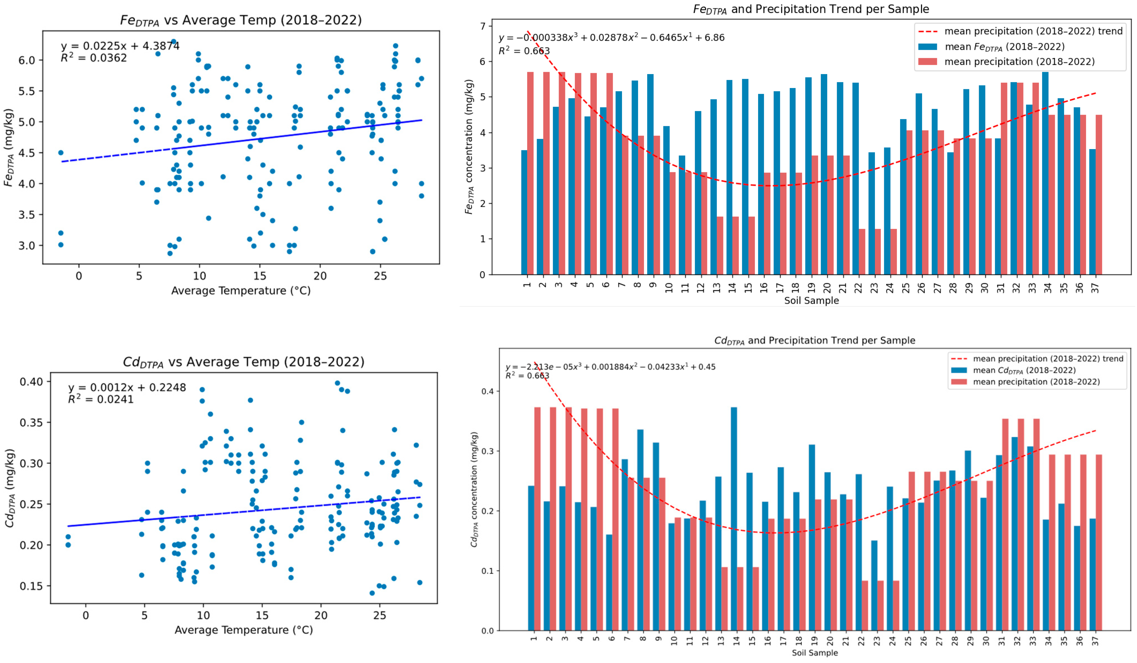
The correlation of the climatic parameters to the available metal concentrations was further investigated through single-variable regression analysis. The plots in Figure 2 provide a dual perspective on the relationship between DTPA-extractable iron ($F{e}_{DTPA}$) and cadmium ($C{d}_{DTPA}$) with climatic parameters—specifically, average temperature and precipitation—during the first half of the study period (2013–2017). The left column shows scatter plots of the available Fe and Cd content against average annual temperature. In both cases, a slight upward trend is visible, but the correlation remains weak, with R² values of 0.05 for Fe and 0.11 for Cd, respectively. These low coefficients of determination indicate that temperature alone cannot reliably explain the observed variation in available metal concentrations. Similar were the findings with other temperature-related features such as the minimum soil temperature $\left(T_{min}\right)$, maximum soil temperature ($T_{max})$ and soil temperature difference ($\mathsf{\Delta }T)$. In contrast, the bar charts on the right, which plot average $F{e}_{DTPA}$ and $C{d}_{DTPA}$ concentrations per sample for the studied year period against mean annual precipitation per soil sample, exhibit more structured trends. Polynomial fits of degree 3 were applied to the precipitation data and compared with DTPA concentrations. For both metals, a U-shaped trend is evident in the precipitation curve, and the bar heights suggest that metal availability increases again in areas with higher rainfall. The R² values of 0.34 indicate moderate explanatory power, suggesting that precipitation, while not solely responsible, may contribute meaningfully to metal mobility or bioavailability, potentially through mechanisms related to leaching or solubilization in wetter conditions.

Figure 3 depicts the corresponding plots for the period 2018–2022. The diagrams reveal both consistent and divergent patterns when compared with those from the earlier 2013–2017 period. In the scatter plots on the left, the relationship between average annual temperature and DTPA-extractable Fe and Cd concentrations remains weak. For $F{e}_{DTPA}$, the R² remains essentially unchanged (0.0493 in both periods), while, for $C{d}_{DTPA}$, it slightly decreases to 0.0241 from 0.1147. These results confirm that average temperature alone does not substantially drive variation in metal bioavailability across years or sampling points.

In contrast, the bar plots on the right—examining mean DTPA metal concentrations and precipitation trends per soil sample—show notable improvements in model fit. Both Fe and Cd now demonstrate a stronger correlation with precipitation trends, with R² values around 0.62–0.63, compared to 0.34 in the earlier period. The precipitation trend lines are modeled with higher-order polynomials, better capturing the non-linear distribution of rainfall across sampling locations. This suggests that precipitation exerted a more pronounced influence on metal availability in the later years. Such a shift may be attributed to increased rainfall variability or to accumulated effects of hydrological changes, which enhance leaching, mobility, or solubilization processes over time.

3.5. Spatial Correlation Trends over Time for Fe/Cd

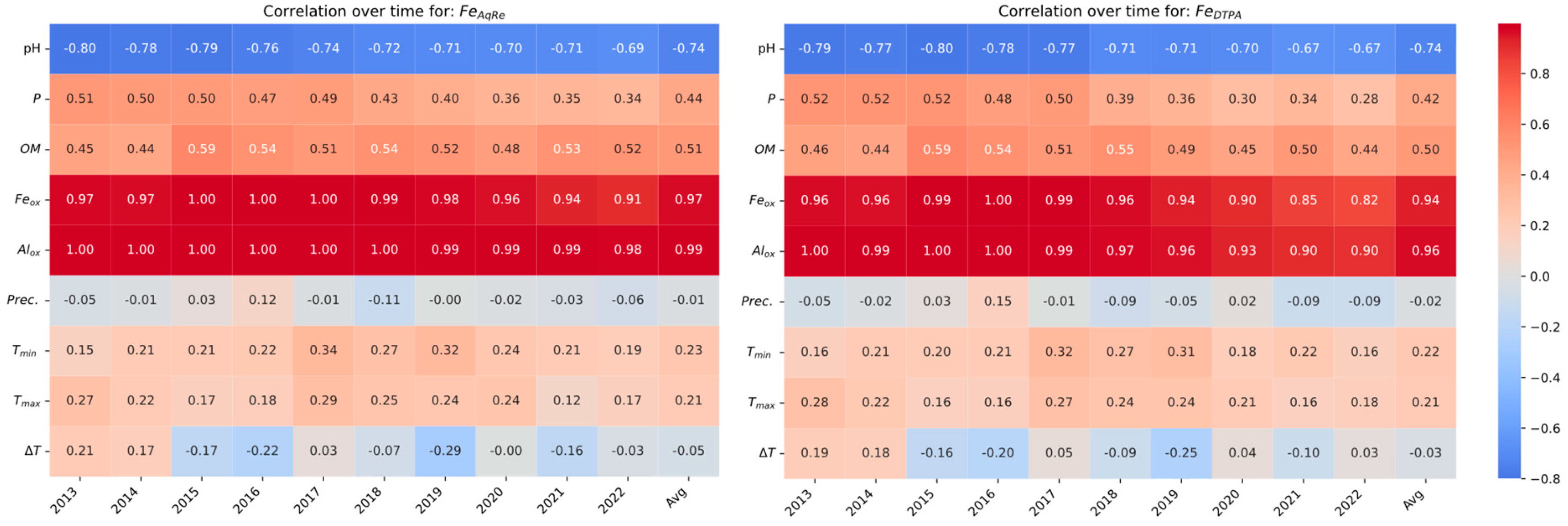
The temporal correlation patterns of the total ($F{e}_{AqRe}$) and DTPA-extractable ($F{e}_{DTPA}$) iron concentrations with a set of selected soil and climatic variables are shown in Figure 4 for the period 2013 to 2022. The correlations are averaged across all samples for each year. The final column shows the average correlation across all years. Warm colors (red) indicate positive correlations, while cool colors (blue) indicate negative correlations.

It is clear that both forms of iron exhibit consistently strong positive correlations with soil oxides, particularly $F{e}_{ox}$ and $A{l}_{ox}$, throughout the decade, underscoring the dominant role of oxide composition in controlling iron availability. Conversely, pH maintains a strong negative correlation with both Fe metrics, aligning with established soil chemistry principles, where higher pH typically reduces metal solubility. The consistent correlation over the years for these elements confirms our findings in [23] for the $F{e}_{AqRe}$. Notably, while total $Fe$ shows relatively stable correlations, $F{e}_{DTPA}$ associations, especially with $F{e}_{ox}$ and $A{l}_{ox}$, appear to weaken slightly in more recent years, possibly due to shifts in external environmental drivers. Importantly, climatic factors such as minimum and maximum temperature ($T_{min}$, $T_{max}$) and precipitation show weaker but non-negligible and sometimes increasing correlations, particularly with $F{e}_{DTPA}$. We also investigated as a climatic feature the mean temperature difference ($\mathsf{\Delta }T=T_{max}-T_{min}$), which did not exhibit strong correlations to the actual metal concentrations. Nevertheless, this suggests that bioavailable iron is more responsive to climatic variability. These trends justify the incorporation of climatic predictors into modeling frameworks, as their subtle but persistent influence can modulate metal dynamics, especially in the context of bioavailability and long-term soil nutrient trends under changing climate conditions.

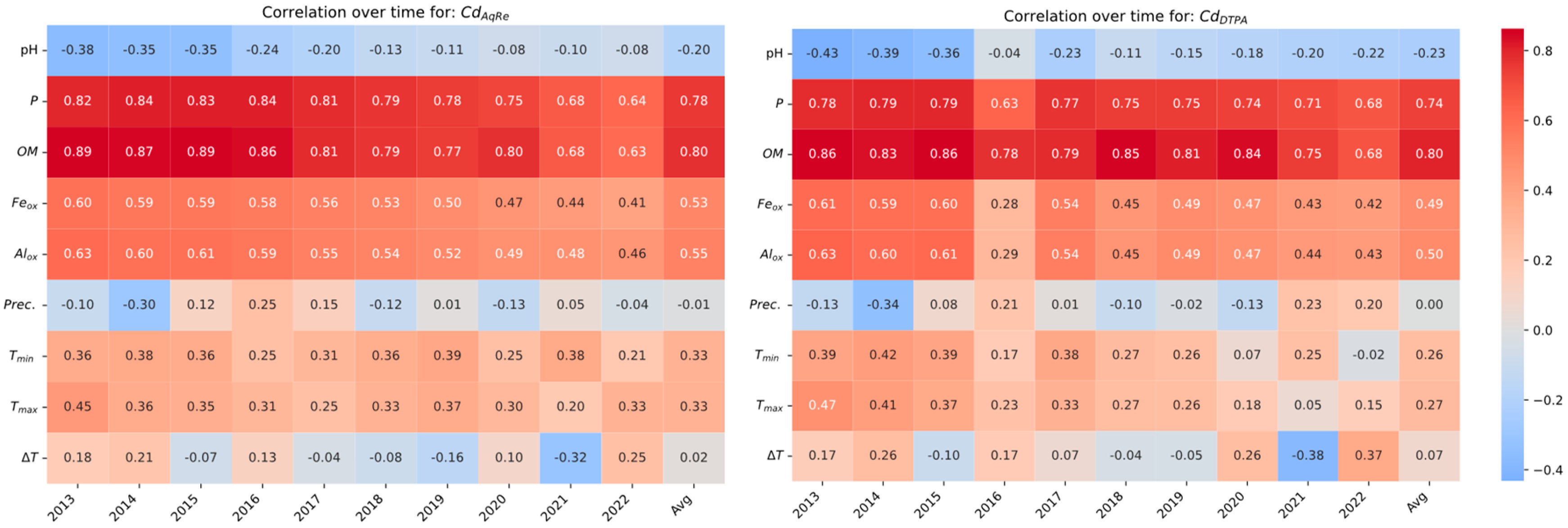
Figure 5 visualizes the corresponding correlation trends for the total and DTPA concentrations of cadmium (${Cd}_{AqRe}$ and ${Cd}_{DTPA}$), revealing key insights into the temporal dynamics of cadmium availability in relation to the soil and climatic variables considered. Again, as expected, organic matter (OM) and phosphorus (P) consistently exhibit strong positive correlations with both forms of cadmium, suggesting their critical roles in cadmium retention and mobility. However, although these strong correlations are retained in earlier years (2013–2017), over time, they progressively decrease to values below 0.7. These shifts suggest that Cd availability in soil is becoming less strongly governed by traditional soil chemical properties. Instead, is it more heavily influenced by other emerging factors including climatic parameters, such as the temperature and the precipitation, since both exhibit a significant increase in their correlation in the last few years of the study. This trend supports the hypothesis that climatic changes could affect the dynamics of cadmium mobility and availability, possibly overriding the control previously exerted by soil composition alone.

3.6. Robust Quadratic Regression (RQR) Prediction of Metal Concentration

In our previous study [21], we applied both multiple robust linear and quadratic regression to an identical dataset covering a five-year period (2013–2018) to develop predictive models for the concentrations of pseudo-total Fe and Cd. The analysis demonstrated that soil pH was the most influential factor affecting total Fe and Cd concentrations. Using multiple quadratic regression, we derived the following regression equations based on 555 samples collected from 37 sites over five years and three sample depths:

For pseudo-total Fe:

$$\mathit{F}\mathit{e}=-\mathbf{196.79}+\mathbf{13.4}\mathit{p}\mathit{H}+\mathbf{9.13}\mathit{F}{\mathit{e}}_{\mathit{o}\mathit{x}}-\mathbf{7.03} \mathit{A}{\mathit{l}}_{\mathit{o}\mathit{x}}-\mathbf{0.48}\mathit{p}\mathit{H}\cdot \mathit{F}{\mathit{e}}_{\mathit{o}\mathit{x}}+\mathbf{0.49}\mathit{p}\mathit{H}\cdot \mathit{A}{\mathit{l}}_{\mathit{o}\mathit{x}}$$

(6)

For pseudo-total Cd:

$$\mathit{C}\mathit{d}=\mathbf{6.45}-\mathbf{1.31} \mathit{p}\mathit{H}-\mathbf{0.34} \mathit{P}+\mathbf{0.49} \mathit{O}\mathit{M}-\mathbf{0.07} \mathit{p}\mathit{H}\cdot \mathit{P}-\mathbf{0.21} \mathit{p}\mathit{H}\cdot \mathit{O}\mathit{M}+\mathbf{0.13} \mathit{P}\cdot \mathit{O}\mathit{M}-\mathbf{0.31} \mathit{O}{\mathit{M}}^{\mathbf{2}}$$

(7)

These equations are highly important, as they link total Fe and Cd concentrations to soil pH and key soil properties, including Fe and Al oxides, soil organic matter (OM), and nutrients such as phosphorus (P) content.

The previously derived equations were validated over the subsequent five years of the study, confirming that the same soil parameters continued to influence total metal concentrations across depths of 0–90 cm. However, the varying availability of Fe and Cd over time prompted further investigation into the factors affecting their available fractions.

A consistent linear relationship was observed between available and total metal concentrations, with available concentrations typically representing about 10% of the total. This pattern was further supported by applying the robust quadratic regression method described in Golia and Diakoloukas (2022) [23]. Using the same primary predictors for total Fe and Cd, and the Huber Robust Regressor we developed the following equations for DTPA-extractable Fe and Cd using the initial five-year dataset:

$$\mathit{F}{\mathit{e}}_{\mathit{D}\mathit{T}\mathit{P}\mathit{A}}=\mathbf{3.49}-\mathbf{0.03}\mathit{p}\mathit{H}+\mathbf{0.37}\mathit{F}{\mathit{e}}_{\mathit{o}\mathit{x}}+\mathbf{0.28} \mathit{A}{\mathit{l}}_{\mathit{o}\mathit{x}}-\mathbf{0.16}\mathit{p}\mathit{H}\cdot \mathit{F}{\mathit{e}}_{\mathit{o}\mathit{x}}+\mathbf{0.41}\mathit{F}{\mathit{e}}_{\mathit{o}\mathit{x}}\cdot \mathit{A}{\mathit{l}}_{\mathit{o}\mathit{x}}-\mathbf{0.28}\mathit{F}{\mathit{e}}_{\mathit{o}\mathit{x}}^{\mathbf{2}}$$

(8)

with $R^{\mathbf{2}}=0.99$ and RMSE = 0.065

$$\mathit{C}{\mathit{d}}_{\mathit{D}\mathit{T}\mathit{P}\mathit{A}}=\mathbf{0.175}+\mathbf{0.001}\mathit{p}\mathit{H}+\mathbf{0.009} \mathit{P}+\mathbf{0.025} \mathit{O}\mathit{M}+\mathbf{0.01} \mathit{p}\mathit{H}\cdot \mathit{P}-\mathbf{0.003} \mathit{p}\mathit{H}\cdot \mathit{O}\mathit{M}$$

(9)

with $R^2=0.76$ and RMSE = 0.02.

These high $R^2$ values, particularly in the case of $F{e}_{DTPA}$, indicate strong model performance, comparable to the results for total metal concentrations presented in Golia and Diakoloukas [21]. Similarly, the low RMSE values indicate minimal prediction errors.

However, when the study was extended for an additional five years (up to 2022), using samples from the same locations, a progressive increase in the deviation between predicted and observed values for both total and available metal concentrations was observed. These deviations, detailed in

Table 4. Comparison of values of available and total concentrations of Fe and Cd. Current measured values and predicted values based on Equations (6)–(9) are compared.

	Real Mean Annual Values				Predicted Mean Annual Values
	FeAqRe	FeDTPA	CdAqRe	Cd DTPA	FeAqRe	FeDTPA	CdAqRe	Cd DTPA
2013	33.25	3.29	1.61	0.158	34.47	3.30	1.628	0.16
2014	33.11	3.39	1.71	0.168	34.92	3.38	1.722	0.168
2015	35.19	3.49	1.789	0.177	35.27	3.49	1.793	0.175
2016	35.98	3.59	1.878	0.186	35.61	3.58	1.87	0.182
2017	36.82	3.68	1.95	0.191	35.39	3.65	1.965	0.192
2018	37.26	4.14	2.013	0.218	36.01	3.74	2.05	0.20
2019	37.66	4.41	2.065	0.231	36.12	3.81	2.136	0.209
2020	38.09	4.76	2.108	0.244	36.4	3.89	2.20	0.215
2021	38.54	5.09	2.162	0.258	36.58	3.96	2.298	0.226
2022	38.93	5.38	2.21	0.269	36.63	4.03	2.40	0.237

, increased annually across all four equations.

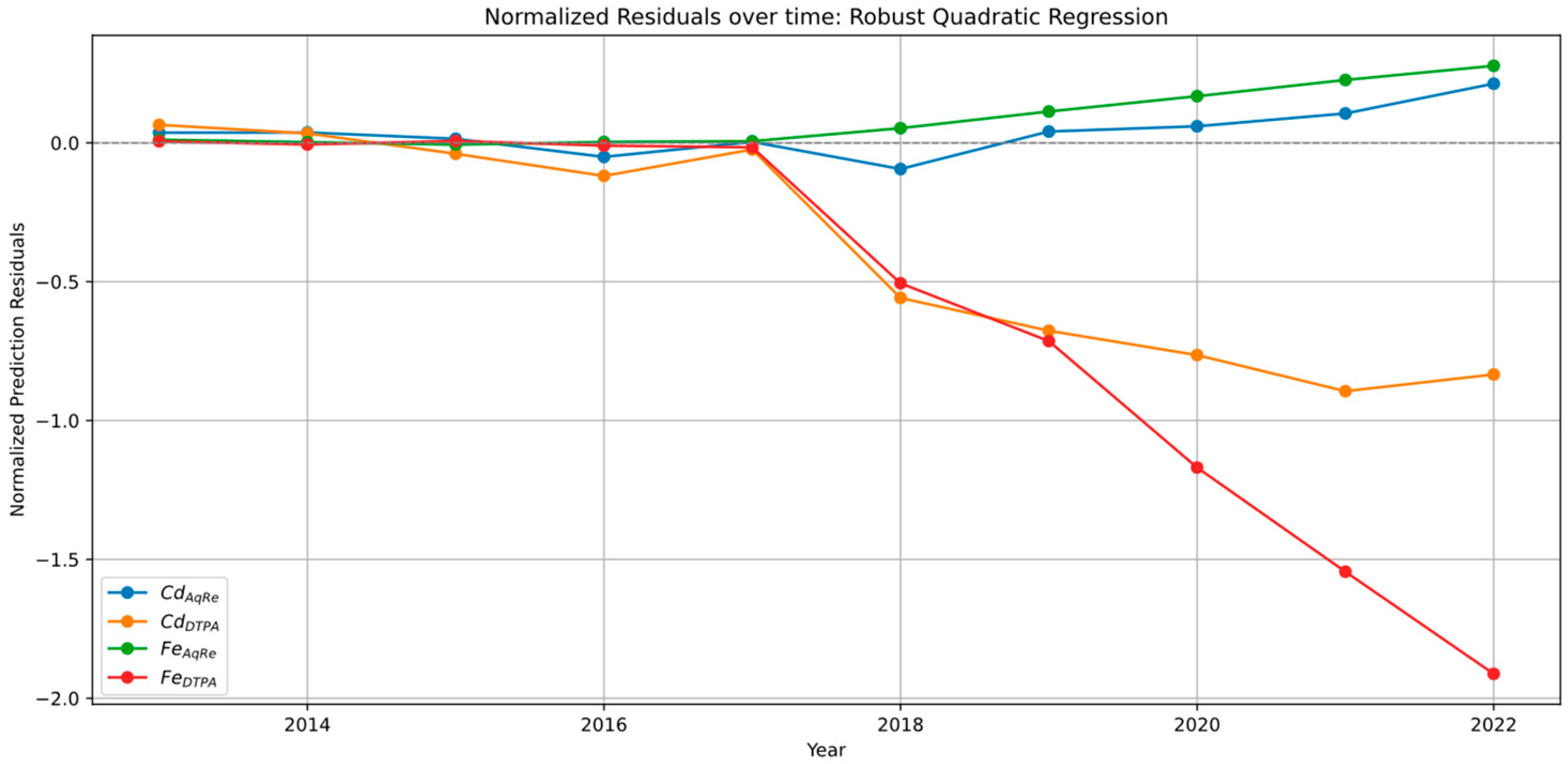
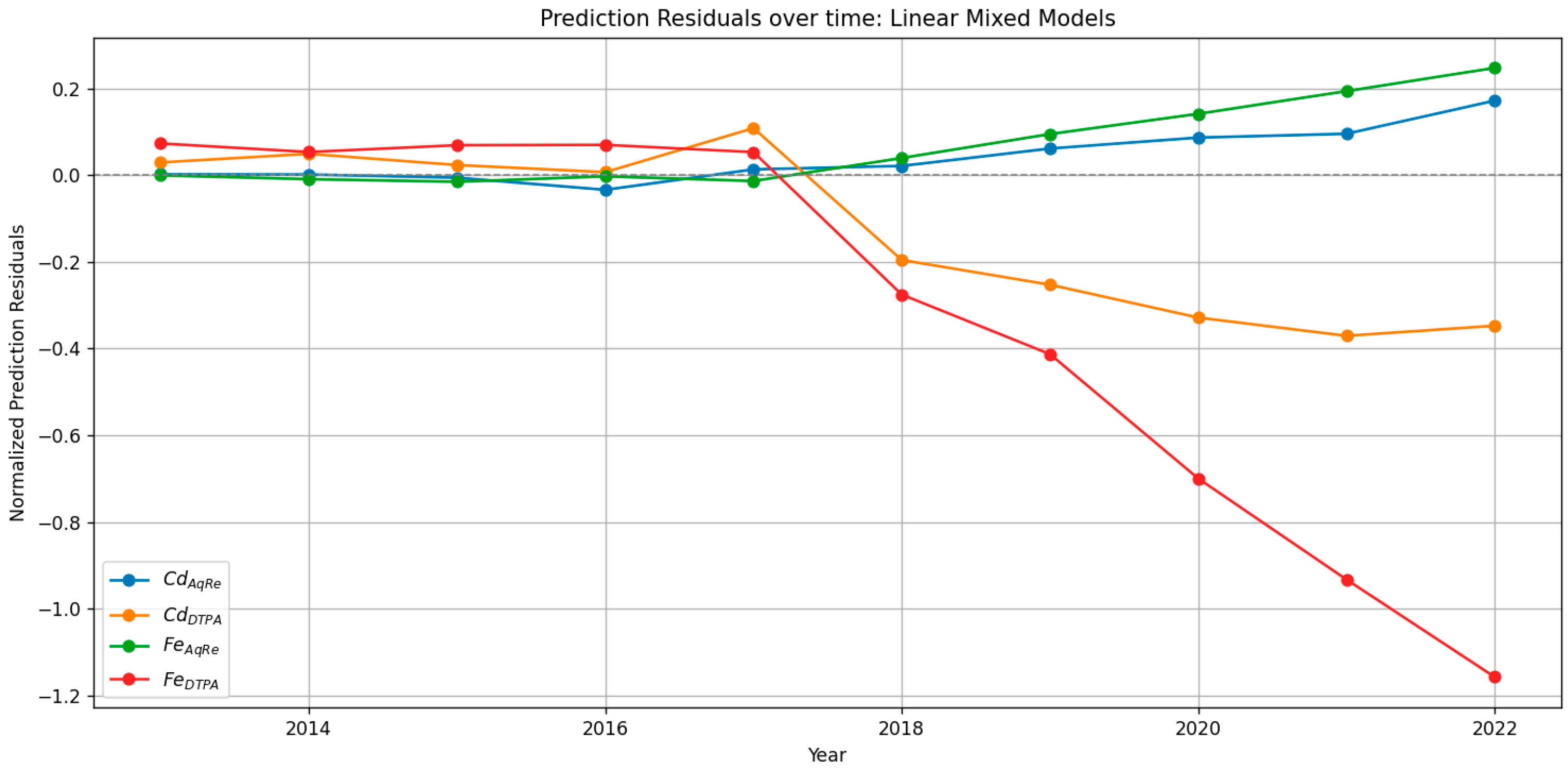
This is better depicted in Figure 6, which shows the average prediction residuals over time for total and DTPA-extractable forms of both metals in the study, using robust quadratic regression (RQR) models trained on early-year data. It should be noted that the residuals were normalized for a fair comparison in the same diagram.

While the residuals for total metal forms remain close to zero or increase slightly over time, those for the DTPA forms exhibit a systematic almost linear decline since 2018, which is mostly notable for the $F{e}_{DTPA}$. This suggests the model’s progressive underestimation of bioavailable metal fractions in recent years. This is likely due to evolving soil or climatic conditions which are not captured during training.

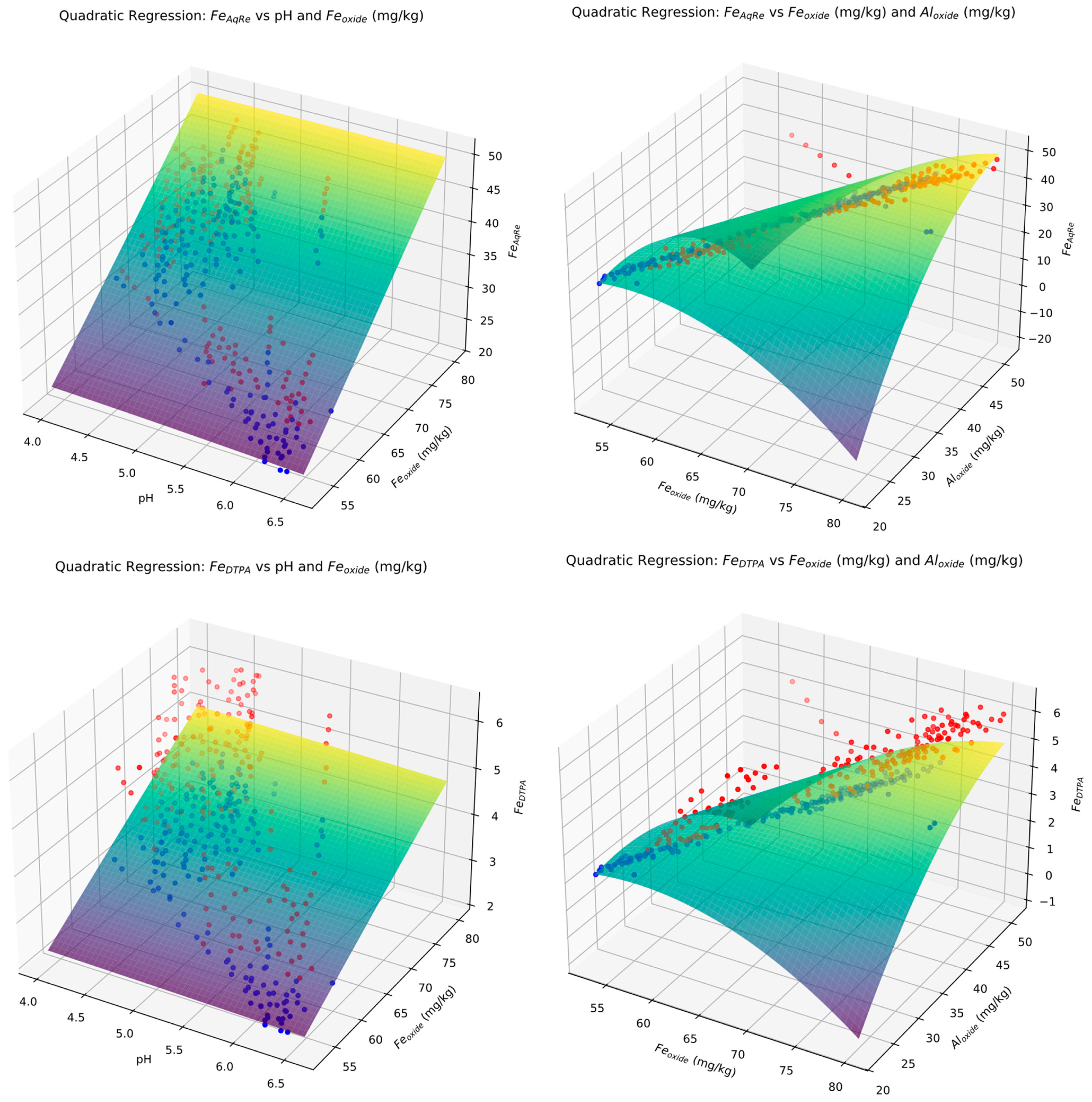
In Figure 7, two out of the total predictors were chosen to obtain 3D visualization of the quadratic regression model for both the total and DTPA forms of Fe concentrations. The training and test samples are also shown in blue and red, respectively. The regression surface (smooth, colored mesh) represents the fitted quadratic model, capturing the nonlinear interaction between the two dependent variables ($pH$ and $F{e}_{oxide}$ in the left column and the oxides of $Fe$ and $Al$ in the right column). The distribution of the red points (test samples corresponding to the years 2018–2022) closely follows the surface; however, there seem to be slight deviations in several cases, particularly in the $F{e}_{DTMA}$ case, underlying moderate predictive performance and generalization.

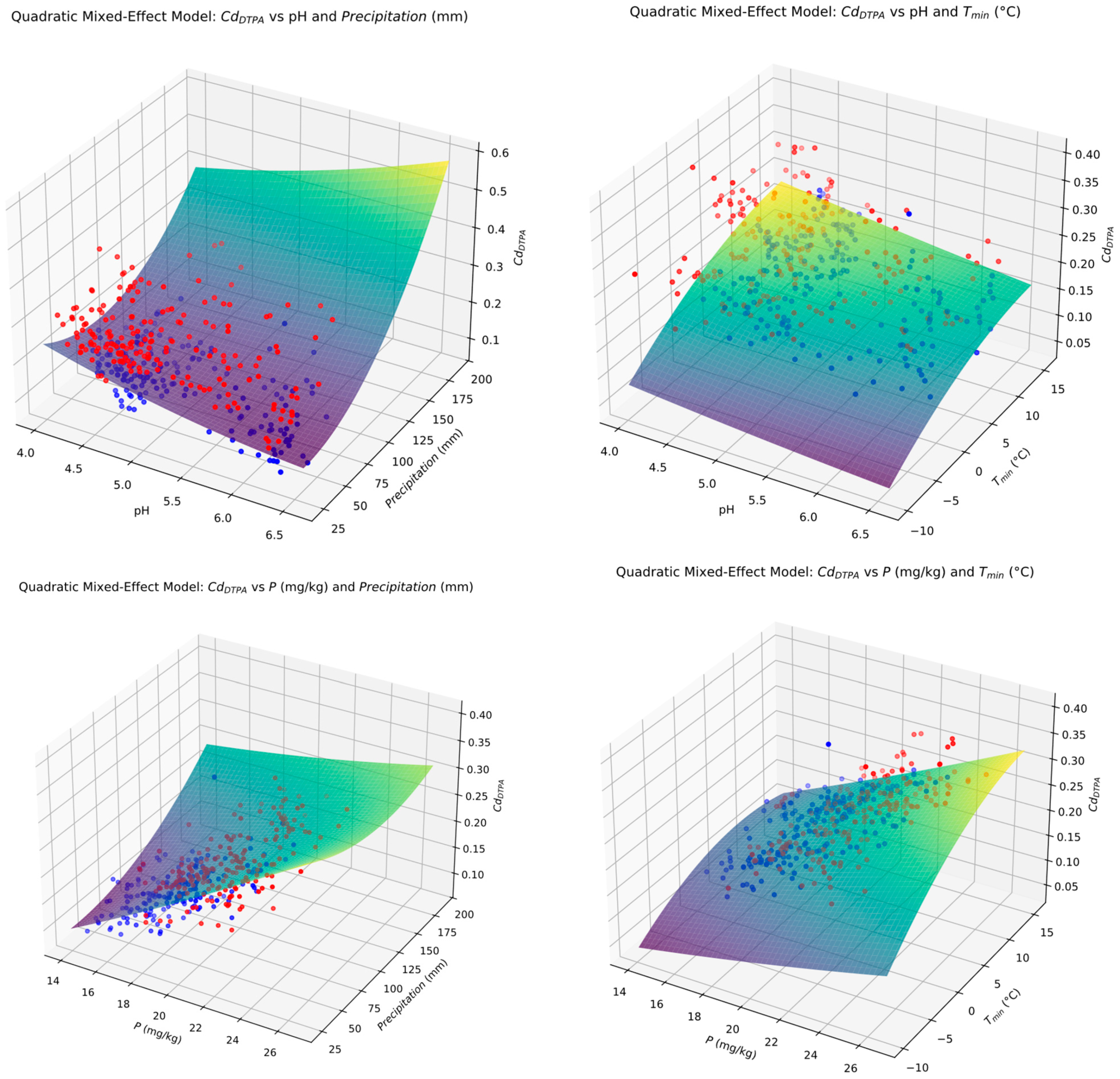
In Figure 8, the corresponding 3D plots for cadmium are depicted. The predictors considered are the $pH$ and phosphorus in the left column and phosphorus and organic matter in the right column. The first row corresponds to the total $C{d}_{AqRe}$ while the last row corresponds to the $C{d}_{DTPA}$. A visual comparison reveals that the total $C{d}_{AqRe}$ exhibits a closer alignment between the test data and the fitted surface, although both cadmium forms are less accurate, particularly in the second column plots, possibly due to predictors that have not been considered.

3.7. Linear Mixed-Effects Model (LMM) Prediction Formulae

As an alternative to the RQR, linear mixed models (LMMs) were trained to predict total and DTPA Fe and Cd concentrations based on soil and climatic parameters. For this training, the parameter of “Year” was treated as a random grouping factor to account for temporal variation. Before applying LMM, the predictor and target variables were normalized using standardization, as in the following equation:

$$x_{i,y}^{std}={\displaystyle \frac{x_{i,y}-{\mu }_i}{{\sigma }_i}},$$

where $x_{i,y}^{std}$ is the standardized values of the parameter $i$ in year $y$, ${\mu }_i$ is the sample mean of the $i-th$ predictor over the training samples and ${\sigma }_i$ is the corresponding standard deviation. In this way, scaling effects due to the different measurement range of the predictors were avoided, ensuring an unbiased model estimation.

The final linear prediction formula for total Fe is:

$$\hspace{1em}\hspace{1em}\hspace{1em}\hspace{1em}\mathit{F}{\mathit{e}}_{\mathit{A}\mathit{q}\mathit{R}\mathit{e}}=-\mathbf{3.4}-\mathbf{0.1}\mathit{p}\mathit{H}+\mathbf{0.15}\mathit{F}{\mathit{e}}_{\mathit{o}\mathit{x}}+\mathbf{0.84} \mathit{A}{\mathit{l}}_{\mathit{o}\mathit{x}}-\mathbf{0.02}{\mathit{T}}_{\mathit{m}\mathit{a}\mathit{x}}$$

(10)

The statistically significant predictors included Fe oxides, Al oxides with a very strong effect (p-value = 0), and the moderately significant maximum temperature (p-value = 0.02) and pH (p-value = 0.16). For the minimum temperature and precipitation, on the other hand, there is no strong evidence of a statistically significant contribution, since their p-values were 0.51 and 0.42, respectively, both greater than the threshold of 0.05. It seems that these climatic variables can be highly correlated, and this multicollinearity might lead to inflated standard errors for the coefficient estimates, which in turn increase the p-values. The model achieved an R² of 0.996 and an RMSE of 0.41, indicating strong predictive performance; however, the climatic variable had a minimal contribution in the model prediction.

The corresponding LMM formula for the DTPA-explainable Fe was found as follows:

$$\mathit{F}{\mathit{e}}_{\mathit{D}\mathit{T}\mathit{P}\mathit{A}}=\mathbf{0.059}-\mathbf{0.012}\mathit{p}\mathit{H}+\mathbf{0.002}\mathit{F}{\mathit{e}}_{\mathit{o}\mathit{x}}+\mathbf{0.099} \mathit{A}{\mathit{l}}_{\mathit{o}\mathit{x}}-\mathbf{0.002}{\mathit{T}}_{\mathit{m}\mathit{a}\mathit{x}}$$

(11)

The model achieved a high goodness-of-fit ($R^2=0.982$) and a low RMSE (0.096), indicating strong explanatory power. Among the predictors, Al oxides (p < 0.001) are the only statistically significant variable at the 95% confidence level, suggesting that they play a crucial role in explaining variability in $F{e}_{DTPA}$. Other variables, such as pH and Fe oxides, though included, do not show statistically significant contributions under the model. This outcome highlights the dominant influence of aluminum oxides in Fe bioavailability and suggests that, while climatic factors are relevant to include due to possible seasonal and environmental effects, their individual contributions may be subtler or confounded with other soil properties.

Similarly, applying LMM to obtain predictions for the total Cd resulted in the following linear equation:

$$\mathit{C}{\mathit{d}}_{\mathit{A}\mathit{q}\mathit{R}\mathit{e}}=-\mathbf{0.722}-\mathbf{0.019}\mathit{p}\mathit{H}+\mathbf{0.086} \mathit{P}+\mathbf{0.539} \mathit{O}\mathit{M}+\mathbf{0.01} {\mathit{T}}_{\mathit{m}\mathit{i}\mathit{n}}-\mathbf{0.002} {\mathit{T}}_{\mathit{m}\mathit{a}\mathit{x}}+\mathbf{0.001}\mathit{P}\mathit{r}\mathit{e}\mathit{c}\mathit{i}\mathit{p}$$

(12)

This equation indicates a strong statistical relationship with certain soil parameters, particularly phosphorus (P) and organic matter (OM) with $p<0.001$. Minimum temperature is also marginally significant ($p\approx 0.08),$ suggesting a potential role in modulating $Cd$ dynamics over time. In contrast, other variables, including pH, maximum temperature and precipitation were not statistically significant, although their inclusion may still help stabilize predictions or interact with other effects.

The corresponding LMM prediction equation for the DTPA-extractable cadmium is formulated as:

$$\mathit{C}{\mathit{d}}_{\mathit{D}\mathit{T}\mathit{P}\mathit{A}}=-\mathbf{0.087}-\mathbf{0.001}\mathit{p}\mathit{H}+\mathbf{0.007} \mathit{P}+\mathbf{0.071} \mathit{O}\mathit{M}-\mathbf{0.001} {\mathit{T}}_{\mathit{m}\mathit{i}\mathit{n}}-\mathbf{0.0002} {\mathit{T}}_{\mathit{m}\mathit{a}\mathit{x}}+\mathbf{0.0001}\mathit{P}\mathit{r}\mathit{e}\mathit{c}\mathit{i}\mathit{p}$$

(13)

The performance metrics show strong predictive power, with an $R^2=0.751$ and a low RMSE of 0.023. As expected, in analogy to the $C{d}_{AqRe}$ model, organic matter (OM) and phosphorus (P) are highly statistically significant ($p<0.001)$ and positively associated with $C{d}_{DTPA}$, serving as major contributors to the mobilization of bioavailable cadmium. The remaining predictors were found to have weaker significance, indicating a limited role; however, they might have an indirect influence on the final prediction.

3.8. Quadratic Mixed Model (QMM) Prediction Formulae

We followed the same standardization process for the variables in the QMM approach because the quadratic terms large-valued predictors could strongly influence the model. Furthermore, since adding quadratic terms in the LMM model resulted in an exponentially increased number of predictors, it is important to filter as many of them as possible. A significant filtering criterion is the multicollinearity, which occurs when two or more predictors are highly correlated, leading to unstable coefficient estimates, inflated standard errors, and unreliable significance testing. Multicollinearity can be detected using the Variance Inflation Factor (VIF), which quantifies the increase in the variance of a regression coefficient due to collinearity. VIF was computed for all polynomial and interaction terms and only retained predictors with a VIF value below a threshold since they should be the most informative ones.

Applying this QMM approach for the total iron concentrations we obtained the following prediction equation:

$$\begin{array}{ll}& \mathit{F}{\mathit{e}}_{\mathit{A}\mathit{q}\mathit{R}\mathit{e}}\\ & =\mathbf{0.103}+\mathbf{0.002}\mathit{P}\mathit{H}+\mathbf{0.949}\mathit{F}{\mathit{e}}_{\mathit{o}\mathit{x}}+\mathbf{0.034}{\mathit{T}}_{\mathit{m}\mathit{i}\mathit{n}}-\mathbf{0.031}{\mathit{T}}_{\mathit{m}\mathit{a}\mathit{x}}-\mathbf{0.112}\mathit{F}{\mathit{e}}_{\mathit{o}\mathit{x}}^{\mathbf{2}}+\mathbf{0.026}\cdot \mathit{A}{\mathit{l}}_{\mathit{o}\mathit{x}}^{\mathbf{2}}+\mathbf{0.035}{\mathit{T}}_{\mathit{m}\mathit{i}\mathit{n}}^{\mathbf{2}}\\ & -\mathbf{0.021}\mathit{F}{\mathit{e}}_{\mathit{o}\mathit{x}}\cdot \mathit{A}{\mathit{l}}_{\mathit{o}\mathit{x}}-\mathbf{0.08}\mathit{P}\mathit{H}\cdot {\mathit{T}}_{\mathit{m}\mathit{i}\mathit{n}}-\mathbf{0.030}\mathit{F}{\mathit{e}}_{\mathit{o}\mathit{x}}\cdot {\mathit{T}}_{\mathit{m}\mathit{a}\mathit{x}}+\mathbf{0.026}{\mathit{A}\mathit{l}}_{\mathit{o}\mathit{x}}\cdot {\mathit{T}}_{\mathit{m}\mathit{a}\mathit{x}}-\mathbf{0.001}\mathit{P}\mathit{r}\mathit{e}\mathit{c}\mathit{i}{\mathit{p}}^{\mathbf{2}}\end{array}$$

(14)

The quadratic model explains more than 98% of the variance with a high goodness-of-fit (R² = 0.981) and a low RMSE (0.12), which indicates excellent predictive accuracy. The quadratic terms permit a better combination of soil and climatic parameters through interactive predictors. For instance, the strong interactions of Fe oxides and Al oxides with maximum temperature show that temperature modulates the effect of these soil elements on total Fe. Minimum temperature is also highly significant, indicating a strong influence on Fe prediction, while precipitation is relatively weak and most of the interactions show borderline or non-significant effects.

The corresponding QMM equation for the DTPA iron concentrations was found as follows:

$$\begin{array}{ll}\mathit{F}{\mathit{e}}_{\mathit{D}\mathit{T}\mathit{P}\mathit{A}}& =\mathbf{0.079}-\mathbf{0.025}\mathit{P}\mathit{H}+\mathbf{0.931}\mathit{F}{\mathit{e}}_{\mathit{o}\mathit{x}}+\mathbf{0.053}{\mathit{T}}_{\mathit{m}\mathit{i}\mathit{n}}+\mathbf{0.031}\mathit{P}{\mathit{H}}^{\mathbf{2}}+\mathbf{0.038}\mathit{F}{\mathit{e}}_{\mathit{o}\mathit{x}}^{\mathbf{2}}+\mathbf{0.017}\mathit{F}{\mathit{e}}_{\mathit{o}\mathit{x}}\cdot \mathit{P}\mathit{r}\mathit{e}\mathit{c}\mathit{i}\mathit{p}\\ & +\mathbf{0.035}{\mathit{T}}_{\mathit{m}\mathit{i}\mathit{n}}^{\mathbf{2}}-\mathbf{0.032}{\mathit{T}}_{\mathit{m}\mathit{a}\mathit{x}}^{\mathbf{2}}+\mathbf{0.029}\mathit{P}\mathit{H}\cdot \mathit{P}\mathit{r}\mathit{e}\mathit{c}\mathit{i}\mathit{p}.-\mathbf{0.062}\mathit{P}\mathit{H}\cdot {\mathit{T}}_{\mathit{m}\mathit{i}\mathit{n}}+\mathbf{0.037}\mathit{P}\mathit{H}\cdot {\mathit{T}}_{\mathit{m}\mathit{a}\mathit{x}}\end{array}$$

(15)

The model achieved a very strong fit with an R² = 0.967 and an RMSE of 0.180, indicating high predictive accuracy. Again, the most critical factor in explaining the extractable $F{e}_{DTPA}$ is the $F{e}_{ox}$. However, non-linear effects of minimum and maximum temperatures and precipitation can also be important. Iron availability appears to depend upon environmental conditions, as indicated by Rajabi et al. [41].

The inclusion of quadratic and interaction terms improves the model’s ability to capture complex environmental effects, making it suited to long-term agricultural or environmental monitoring.

The QMM regression equation for the total cadmium was found to be:

$$\begin{array}{ll}{\mathit{C}\mathit{d}}_{\mathit{A}\mathit{q}\mathit{R}\mathit{e}}=& -\mathbf{0.004}+\mathbf{0.330}\mathit{P}+\mathbf{0.953}\mathit{O}\mathit{M}+\mathbf{0.165}{\mathit{P}}^{\mathbf{2}}+\mathbf{0.244}\mathit{P}\mathit{H}{\cdot \mathit{T}}_{\mathit{m}\mathit{i}\mathit{n}}-\mathbf{0.230}\mathit{P}\mathit{H}\cdot {\mathit{T}}_{\mathit{m}\mathit{a}\mathit{x}}+\mathbf{0.175}\cdot \mathit{O}\mathit{M}\\ & \cdot {\mathit{T}}_{\mathit{m}\mathit{i}\mathit{n}}+\mathbf{0.142}\mathit{P}\mathit{H}\cdot \mathit{P}+\mathbf{0.075}\mathit{P}\mathit{H}\cdot \mathit{P}\mathit{r}\mathit{e}\mathit{c}.+\mathbf{0.086}{\mathit{P}}^{\mathbf{2}}+\mathbf{0.092}{\mathit{T}}_{\mathit{m}\mathit{i}\mathit{n}}^{\mathbf{2}}\end{array}$$

(16)

In the above equation, only the significant terms were retained. The model achieves $R^2=0.867$ and RMSE = 0.363, suggesting a relatively good predictive error. $C{d}_{AqRe}$ is significantly influenced by a mix of linear, quadratic, and interaction terms. The linear terms for $P$ and $OM$ are highly significant, indicating strong positive effects. In addition, the climatic parameters exhibit a significant contribution based on their nonlinear relationships and conditional dependencies with several soil parameters such as PH. Li et al. [42], studying soil Cd levels in cultivated rice, drew conclusions showing a tight relationship between Cd availability and soil acidity.

The inclusion of such quadratic and interaction terms seem to enhance model flexibility and can better explain the indirect effect of climatic parameters in the prediction. On the other hand, the small group variance (<0.1) shows that random effects do not explain further variability after accounting for the included predictors.

Finally, the corresponding quadratic form of the DTMA-explainable cadmium predictor was estimated as:

$$\begin{array}{ll}{\mathit{C}\mathit{d}}_{\mathit{D}\mathit{T}\mathit{P}\mathit{A}}& = -\mathbf{0.09}+\mathbf{0.213}\mathit{P}+\mathbf{0.547}\mathit{O}\mathit{M}+\mathbf{0.275}\mathit{P}\mathit{H}\cdot \mathit{P}-\mathbf{0.28} \mathit{P}\mathit{H}{\cdot \mathit{T}}_{\mathit{m}\mathit{a}\mathit{x}}+\mathbf{0.101}\mathit{P}{\mathit{H}}^{\mathbf{2}}+\mathbf{0.191}{\mathit{P}}^{\mathbf{2}}\\ & -\mathbf{0.065}{\mathit{O}\mathit{M}}^{\mathbf{2}}-\mathbf{0.109}{\mathit{T}}_{\mathit{m}\mathit{i}\mathit{n}}^{\mathbf{2}}+\mathbf{0.243} \mathit{P}\mathit{H}{\cdot \mathit{T}}_{\mathit{m}\mathit{i}\mathit{n}}+\mathbf{0.125}\mathit{P}\cdot {\mathit{T}}_{\mathit{m}\mathit{i}\mathit{n}}+\mathbf{0.275}\mathit{P}\mathit{H}\cdot \mathit{P}+\mathbf{0.275} \mathit{P}\mathit{H}\cdot \mathit{P}\end{array}$$

(17)

Again, only coefficients with $p<0.05$ were retained. The model achieves $R^2=0.812$, indicating good explanatory power, and RMSE = 0.433, suggesting moderate predictive error. Soil organic matter (OM) and phosphorus are highly significant predictors. Phosphorus, OM and pH are also significant both as quadratic effects and in terms of their interactions with other soil and climatic parameters and the same stands for minimum temperature as the most influential climatic parameter.

The soil–climatic parameter interactions in the above equations can also serve as strong indicators regarding the influence of the climate in metal availability. For instance, in the $C{d}_{DTPA}$ QMM equation, the negative coefficient of the interactive predictor $PH\cdot T_{max}$ suggests that low temperatures could enhance cadmium availability under acidic soil conditions. Wu et al. [43] studied the conceivable changes in soil organic matter levels when temperature fluctuations are experienced in the soil environment.

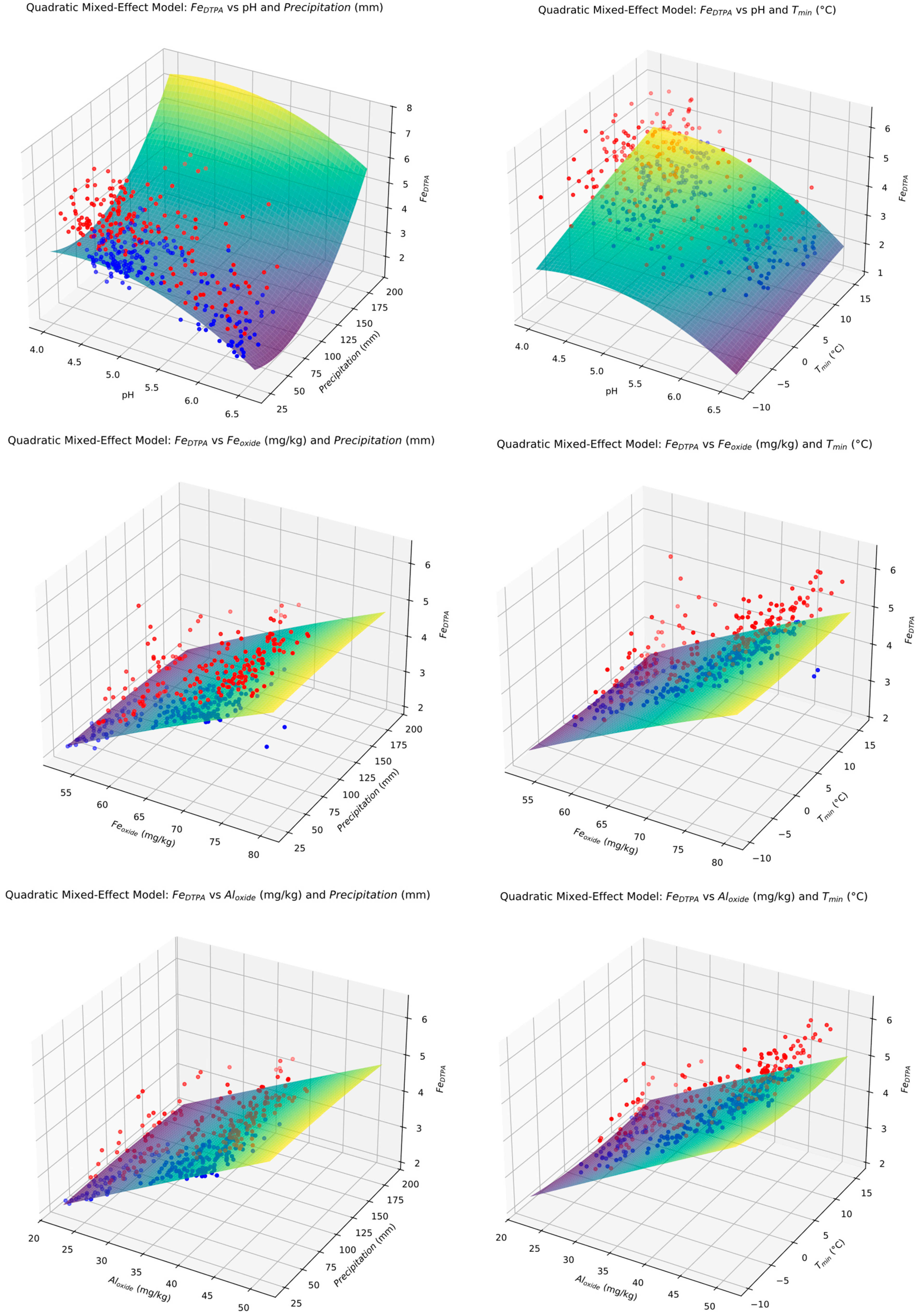
The 3D surface plots in Figure 9 offer a comprehensive visualization of the response surface generated by the QMM model for $F{e}_{DTPA}$ concentrations, using combinations of soil-related and climatic predictors. Each subplot illustrates how interactions between $pH$, $F{e}_{oxide}$, $A{l}_{oxide}$, precipitation, and minimum temperature ($Tmin$) influence the predicted availability of iron.

A common pattern across these visualizations is the nonlinear interaction between soil acidity (pH) and climate factors (precipitation or $Tmin$), which demonstrates a pronounced curvature—indicating that the effect of climate variables on Fe availability is not uniform across all soil conditions. For instance, in the top-left plot ($F{e}_{DTPA}$ vs. pH and Precipitation), the surface peaks at moderate pH and precipitation values, suggesting optimal mobilization of Fe under intermediate conditions. Similarly, in the top-right plot ($F{e}_{DTPA}$ vs. pH and $Tmin$), the elevated $Tmin$ enhances $Fe$ availability primarily in moderately acidic soils.

The bottom two plots ($F{e}_{DTPA}$ vs. $F{e}_{oxide}$ or $A{l}_{oxide}$ with climate variables) confirm that oxide forms of $Fe$ and $Al$ significantly drive $F{e}_{DTPA}$ predictions, especially when modulated by environmental parameters. Notably, the slope steepens along the climate dimension, which supports the hypothesis that long-term changes in precipitation or $Tmin$ may critically alter $Fe$ availability through synergistic effects with mineral fractions, as Reis et al. [44] also concluded in their research.

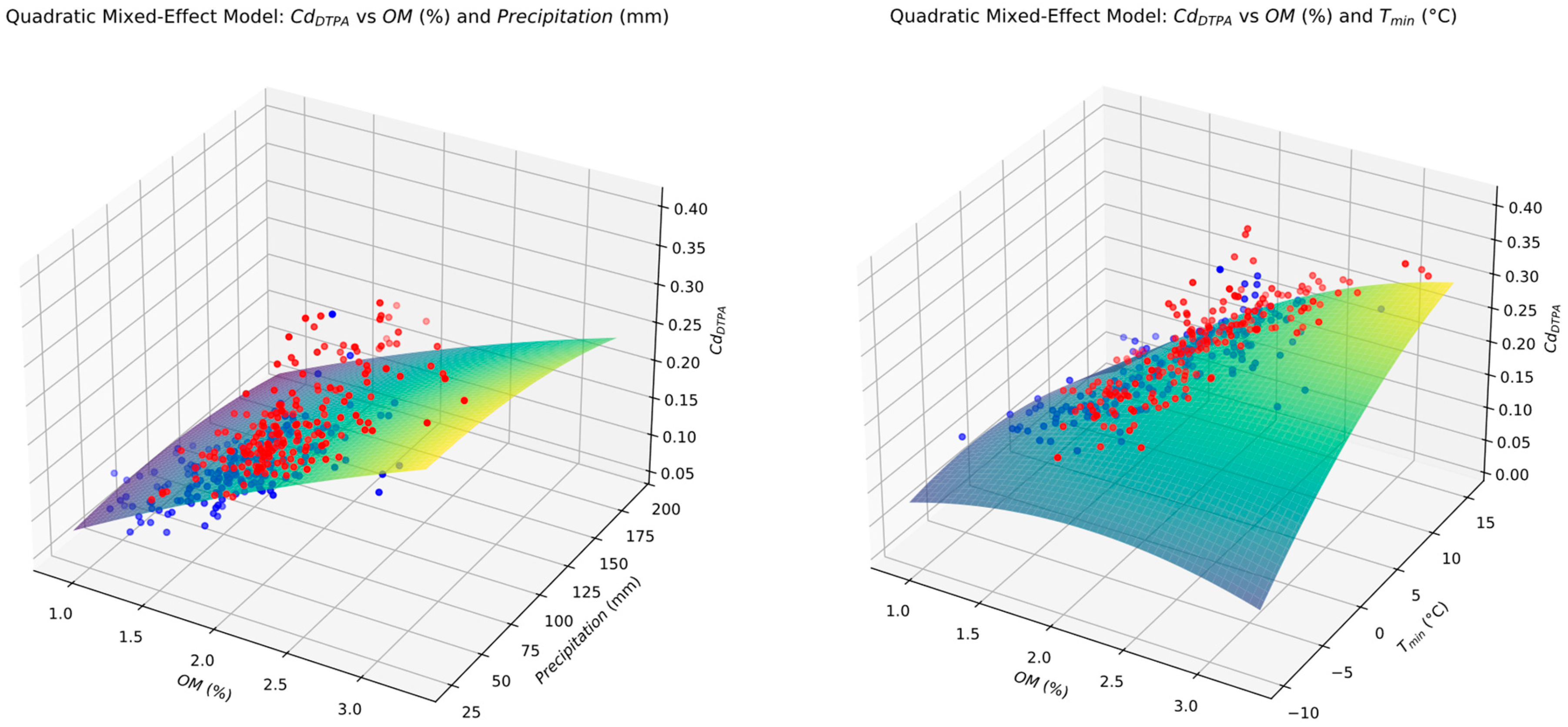
The six surface plots in Figure 10 depict the results of a quadratic mixed-effects model applied to predict $C{d}_{DTPA}$ concentrations using interactions between soil and climatic parameters. Overall, the surfaces exhibit higher non-linearity than the corresponding $F{e}_{DTPA}$ shown previously in Figure 9, particularly in response to precipitation. This suggests that cadmium availability may initially decline with increasing precipitation before rising again, likely reflecting thresholds in leaching, mobilization, or sorption processes. Shang et al. [45] studied the transformations occurring in the availability of toxic elements such as Cd when subjected to temperature and climatic alterations in the environment.

Similarly, the $Tmin$ plots also reveal non-linear responses, which suggest that cadmium mobility is highly sensitive mostly to the interactions of climatic parameters with soil chemistry. Encouragingly, in all 3D diagrams for both metals, the red points that represent test samples in the late years fall relatively closely along the fitted surfaces in most cases. This reflects the good generalization capacity of the models even in more complex non-linear behaviors. It also highlights the benefit of using quadratic regression forms, which better accommodate such complexities without overfitting.

3.9. LMM and QMM Residuals

As shown in the residual plot for the robust quadratic regression (RQR) model in Figure 3, although the model is, by design, more resilient to outliers, it exhibits significant deteriorating trends after 2017, indicating possible influence from climatic parameters. In particular, $F{e}_{DTPA}$ shows increasing negative residuals, implying a consistent underestimation in later years. While being extremely stable in the early years, it ultimately fails to maintain accuracy in the long term.

Figure 11 and Figure 12 present the corresponding normalized residual diagrams over time for the linear and quadratic mixed-effects model predictors (LMM and QMM). The LMM plot reveals similar divergence beginning after 2017, especially for $F{e}_{DTPA}$ and $C{d}_{DTPA}$. Although its form resembles that of the RQR model, the slope of the relatively linear deterioration after 2018 is less steep, resulting in lower residuals for both metals in the ending year of 2022. Nevertheless, the increasing deviation from zero in the later years indicates a declining model performance, which possibly fails to capture the time-dependent effects. The linear assumption of the model seems to be inadequate in providing the necessary flexibility.

On the other hand, the residual trends of the QMM in Figure 12 exhibit a minimally deviating, almost flat line over the years, since the normalized residuals remain tightly clustered around zero. The small fluctuations do not indicate systematic over- or under-prediction trends, demonstrating the ability of the QMM approach to generalize well to future years based on both the soil and climatic parameters and their quadratic and interacting terms.

4. Conclusions

This study was initiated in response to the observed increase in Aqua-Regia-extracted total and DTPA-extracted available concentrations of iron (Fe) and cadmium (Cd) in the agricultural soils of the Thessalian Plain over a ten-year period (2013–2022). Both concentrations maintained an approximate availability ratio of 0.1, with both metals exhibiting a slight but consistent increase over time. Given this temporal trend, the primary objective was to investigate whether climatic parameters, specifically temperature and precipitation, contributed to this variation, and whether their interactions with key soil properties could enhance the accuracy of predictive models for both total and DTPA-extractable metal concentrations.

The spatiotemporal analysis of correlations revealed a gradual weakening of traditional soil–metal associations and a growing influence of temperature and precipitation. This reinforces the need to investigate robust prediction models that can accommodate evolving soil–climate–metal dynamics, particularly under the influence of ongoing climatic shifts.

To address this, we successfully developed and evaluated three regression-based modeling approaches: robust quadratic regression (RQR), linear mixed models (LMMs) and quadratic mixed models (QMMs). These models incorporated both soil variables and climatic predictors (i.e., minimum and maximum temperature and precipitation) to estimate the total and available concentrations of iron (Fe) and cadmium (Cd) in agricultural soils. The residual analysis provided critical insight into model robustness, with QMM being the most accurate and resilient against overfitting and temporal drift. Specifically, QMM achieved R² up to 0.981 for total Fe and 0.967 for DTPA-Fe, with low RMSE values (0.12 and 0.18, respectively). For Cd, QMM explained 86.7% of the variance for total Cd and 81.2% for DTPA-extractable Cd, outperforming both RQR and LMM. Residual trends further confirmed that QMM maintained minimal bias over time, in contrast to the LMM and RQR models, which showed clear deterioration after 2017.

Furthermore, in this study, we show that, while individual climatic variables such as temperature and precipitation might not show consistently strong linear correlations with metal concentrations on a yearly basis, their quadratic interactions with soil properties proved to be statistically significant and predictive when modeled over longer timeframes. This finding underscores the importance of considering nonlinear relationships and mixed-effects structures in environmental prediction tasks.

With the Thessalian Plain representing a critical agricultural region in Greece, such models are not only academically valuable but also practical tools for guiding sustainable soil management and policy decisions. Continued monitoring and data enrichment will be essential for refining these models and responding to future environmental challenges, including extreme events such as the floods of September 2023.

References

1. Arafin, S.A.K.; Fazlul Hoque, A.K.M.; Abedin, M.J.; El-Taher, A. Heavy Metal Detection in Soil and Related Health Aspect at Aila Inundated Sundarban Region, Bangladesh. Int. J. Sci. Technol. Res. 2019, 8, 2702–2708. [Google Scholar]
2. Luo, N. Methods for Controlling Heavy Metals in Environmental Soils Based on Artificial Neural Networks. Sci. Rep. 2024, 14, 2563. [Google Scholar] [CrossRef] [PubMed]
3. Sodango, T.H.; Li, X.; Sha, J.; Bao, Z. Review of the Spatial Distribution, Source and Extent of Heavy Metal Pollution of Soil in China: Impacts and Mitigation Approaches. J. Health Pollut. 2018, 8, 53–70. [Google Scholar] [CrossRef] [PubMed]
4. Golia, E.E.; Emmanouil, C.; Charizani, A.; Koropouli, A.; Kungolos, A. Assessment of Cu and Zn Contamination and Associated Human Health Risks in Urban Soils from Public Green Spaces in the City of Thessaloniki, Northern Greece. Euro-Mediterr. J. Environ. Integr. 2023, 8, 517–525. [Google Scholar] [CrossRef]
5. Schwanen, C.A.; Stauch, G.; Schulte, P.; Schwarzbauer, J. Reconstruction of the Pollution History of the Urft Reservoir: An Organic-Geochemical Investigation. Environ. Sci. Eur. 2024, 36, 103. [Google Scholar] [CrossRef]
6. Zhao, H.; Wu, Y.; Lan, X.; Yang, Y.; Wu, X.; Du, L. Comprehensive Assessment of Harmful Heavy Metals in Contaminated Soil in Order to Score Pollution Level. Sci. Rep. 2022, 12, 3552. [Google Scholar] [CrossRef]
7. Qi, D.; Chen, H.; Hu, L.; Sun, J. Multimethod Analysis of Heavy Metal Pollution and Source Apportionment in a Southeastern Chinese Region. Appl. Sci. 2024, 14, 10559. [Google Scholar] [CrossRef]
8. Golia, E.E.; Bethanis, J.; Xagoraris, C.; Tziourrou, P. Potentially Toxic Elements in Urban and Peri-Urban Soils—A Critical Meta-Analysis of Their Sources, Availability, Interactions, and Spatial Distribution. J. Ecol. Eng. 2024, 25, 335–350. [Google Scholar] [CrossRef]
9. Chen, F.; Chen, X.; Zhu, F.; Sun, Q. Study on the Factors Affecting the Spatial Distribution of Heavy Metal Elements. IOP Conf. Ser. Earth Environ. Sci. 2019, 330, 042013. [Google Scholar] [CrossRef]
10. Onwuka, B. Effects of Soil Temperature on Some Soil Properties and Plant Growth. Adv. Plants Agric. Res. 2018, 8, 34–37. [Google Scholar] [CrossRef]
11. Xu, H.; Huang, L.; Chen, J.; Zhou, H.; Wan, Y.; Qu, Q.; Wang, M.; Xue, S. Changes in Soil Microbial Activity and Their Linkages with Soil Carbon under Global Warming. Catena 2023, 232, 107419. [Google Scholar] [CrossRef]
12. Sun, W.; Li, S.; Zhang, G.; Fu, G.; Qi, H.; Li, T. Effects of Climate Change and Anthropogenic Activities on Soil PH in Grassland Regions on the Tibetan Plateau. Glob. Ecol. Conserv. 2023, 45, e02532. [Google Scholar] [CrossRef]
13. Sebola Tshisikhawe, C.; Ngole-Jeme, V.M. Temperature Induced Changes on Heavy Metal Geochemical Partitioning and Mobility in Contaminated and Uncontaminated Soils. Environ. Pollut. Bioavailab. 2024, 36, 2317747. [Google Scholar] [CrossRef]
14. Biswas, B.; Qi, F.; Biswas, J.K.; Wijayawardena, A.; Khan, M.A.I.; Naidu, R. The Fate of Chemical Pollutants with Soil Properties and Processes in the Climate Change Paradigm—A Review. Soil Syst. 2018, 2, 51. [Google Scholar] [CrossRef]
15. Cornu, J.-Y.; Denaix, L.; Lacoste, J.; Sappin-Didier, V.; Nguyen, C.; Schneider, A. Impact of Temperature on the Dynamics of Organic Matter and on the Soil-to-Plant Transfer of Cd, Zn and Pb in a Contaminated Agricultural Soil. Environ. Sci. Pollut. Res. 2016, 23, 2997–3007. [Google Scholar] [CrossRef]
16. Papadimou, S.G.; Golia, E.E.; Barbayiannis, N.; Tsiropoulos, N.G. Dual Role of the Hyperaccumulator Silybum Marianum (L.) Gaertn. in Circular Economy: Production of Silymarin, a Valuable Secondary Metabolite, and Remediation of Heavy Metal Contaminated Soils. Sustain. Chem. Pharm. 2024, 38, 101454. [Google Scholar] [CrossRef]
17. Elferjani, R.; Soolanayakanahally, R. Canola Responses to Drought, Heat, and Combined Stress: Shared and Specific Effects on Carbon Assimilation, Seed Yield, and Oil Composition. Front. Plant Sci. 2018, 9, 1224. [Google Scholar] [CrossRef]
18. Bayraklı, B.; Dengiz, O.; Özyazıcı, M.A.; Koç, Y.; Kesim, E.; Türkmen, F. Assessment of Heavy Metal Concentrations and Behavior in Cultivated Soils under Humid-Subhumid Environmental Condition of the Black Sea Region. Geoderma Reg. 2023, 32, e00593. [Google Scholar] [CrossRef]
19. Peng, L.; Liu, P.; Feng, X.; Wang, Z.; Cheng, T.; Liang, Y.; Lin, Z.; Shi, Z. Kinetics of Heavy Metal Adsorption and Desorption in Soil: Developing a Unified Model Based on Chemical Speciation. Geochim. Cosmochim. Acta 2018, 224, 282–300. [Google Scholar] [CrossRef]
20. Wijngaard, R.R.; van der Perk, M.; van der Grift, B.; de Nijs, T.C.M.; Bierkens, M.F.P. The Impact of Climate Change on Metal Transport in a Lowland Catchment. Water Air Soil Pollut. 2017, 228, 107. [Google Scholar] [CrossRef]
21. Taghizadeh-Mehrjardi, R.; Schmidt, K.; Amirian-Chakan, A.; Zeraatpisheh, M.; Valavi, R.; Davatgar, N.; Heung, B.; Johnson, M.S.; Mosavi, A. Modelling the spatial–temporal variation of multiple heavy metals in the soil of a large catchment using a random forest model. Remote Sens. 2021, 13, 1698. [Google Scholar] [CrossRef]
22. Keçeci, M.; Gökmen, F.; Usul, M.; Koca, C.; Uygur, V. Prediction of Cadmium Content Using Machine Learning Methods. Environ. Earth Sci. 2024, 82, 12. [Google Scholar] [CrossRef]
23. Golia, E.E.; Diakoloukas, V. Soil Parameters Affecting the Levels of Potentially Harmful Metals in Thessaly Area, Greece: A Robust Quadratic Regression Approach of Soil Pollution Prediction. Environ. Sci. Pollut. Res. 2022, 29, 29544–29561. [Google Scholar] [CrossRef] [PubMed]
24. Page, A.L. Methods of Soil Analysis-Part 2: Chemical and Microbiological Properties, 2nd ed.; American Society of Agronomy, Inc.: Madison, MI, USA, 1982; Volume 9, pp. 421–422. [Google Scholar]
25. Lindsay, W.; Norvell, W.A. Development of a DTPA Soil Test for Zinc, Iron, Manganese, and Copper. Soil Sci. Soc. Am. J. 1978, 42, 421–428. [Google Scholar] [CrossRef]
26. ISO/DIS 11466.(1994); Environment Soil Quality. ISO Standards Compendium: Geneva, Switzerland, 1994.
27. Arkes, J. Regression Analysis; Routledge: London, UK, 2019; ISBN 9781351011099. [Google Scholar]
28. Kuchibhotla, A.K.; Brown, L.D.; Buja, A.; Cai, J. All of Linear Regression. arXiv 2019, arXiv:1910.06386. [Google Scholar]
29. Yu, C.; Yao, W. Robust Linear Regression: A Review and Comparison. Commun. Stat. Simul. Comput. 2017, 46, 6261–6282. [Google Scholar] [CrossRef]
30. Green, P.J. Iteratively Reweighted Least Squares for Maximum Likelihood Estimation, and Some Robust and Resistant Alternatives. J. R. Stat. Soc. Ser. B Stat. Methodol. 1984, 46, 149–170. [Google Scholar] [CrossRef]
31. Wang, Y.-G.; Lin, X.; Zhu, M.; Bai, Z. Robust Estimation Using the Huber Function with a Data-Dependent Tuning Constant. J. Comput. Graph. Stat. 2007, 16, 468–481. [Google Scholar] [CrossRef]
32. Feng, Y.; Wu, Q. A Statistical Learning Assessment of Huber Regression. J. Approx. Theory 2022, 273, 105660. [Google Scholar] [CrossRef]
33. West, B.T.; Welch, K.B.; Galecki, A.T. Linear Mixed Models; Chapman and Hall/CRC: Boca Raton, FL, USA, 2006; ISBN 9780429186554. [Google Scholar]
34. Montesinos López, O.A.; Montesinos López, A.; Crossa, J. Linear Mixed Models. In Multivariate Statistical Machine Learning Methods for Genomic Prediction; Springer International Publishing: Cham, Switzerland, 2022; pp. 141–170. [Google Scholar]
35. Bolker, B.M.; Brooks, M.E.; Clark, C.J.; Geange, S.W.; Poulsen, J.R.; Stevens, M.H.H.; White, J.-S.S. Generalized Linear Mixed Models: A Practical Guide for Ecology and Evolution. Trends Ecol. Evol. 2009, 24, 127–135. [Google Scholar] [CrossRef]
36. Ojo, A.O.; Nwosu, N.J.; Oshunsanya, S.O.; Ayantayo-Ojo, V.I.; Aladele, S.E. Impacts of Soil Conservation Techniques on Soil Erodibility on an Alfisol. Heliyon 2023, 9, e13768. [Google Scholar] [CrossRef]
37. Debnath, J.; Sow, P.; Kundu, M.C. Variation of PH Dependent Acidity and Total Potential Acidity as Influenced by Land Uses and Soil Depths in Lateritic Belt of West Bengal. Int. J. Curr. Microbiol. Appl. Sci. 2021, 10, 1289–1298. [Google Scholar] [CrossRef]
38. Gök, G.; Tulun, Ş.; Çelebi, H. Mapping of Heavy Metal Pollution Density and Source Distribution of Campus Soil Using Geographical Information System. Sci. Rep. 2024, 14, 29918. [Google Scholar] [CrossRef]
39. Bouslihim, Y.; John, K.; Miftah, A.; Azmi, R.; Aboutayeb, R.; Bouasria, A.; Razouk, R.; Hssaini, L. The Effect of Covariates on Soil Organic Matter and PH Variability: A Digital Soil Mapping Approach Using Random Forest Model. Ann. GIS 2024, 30, 215–232. [Google Scholar] [CrossRef]
40. Badagliacca, G.; Lo Presti, E.; Gelsomino, A.; Monti, M. Repeated Solid Digestate Amendment Increases Denitrifying Enzyme Activity in an Acid Clayey Soil. Soil Syst. 2024, 8, 14. [Google Scholar] [CrossRef]
41. Rajabi Hamedani, S.; Cardarelli, M.; Rouphael, Y.; Bonini, P.; Colantoni, A.; Colla, G. Comparative Environmental Assessment of the Iron Fertilisers’ Production: Fe-Biochelate versus Fe-EDDHA. Sustainability 2023, 15, 7488. [Google Scholar] [CrossRef]
42. Li, E.; Li, K.; Li, J.; Wu, Y.; Ma, Y. A New Approach to Differentiate the Causes of Excessive Cadmium in Rice: Soil Cadmium Extractability or Rice Variety. Agronomy 2024, 14, 2519. [Google Scholar] [CrossRef]
43. Wu, Y.; Li, H.; Liang, X.; Jiang, M.; He, S.; He, Y. Mechanisms Behind the Soil Organic Carbon Response to Temperature Elevations. Agriculture 2025, 15, 1118. [Google Scholar] [CrossRef]
44. Reis, A.R.; Roboredo, M.; Pinto, J.P.R.M.; Vieira, B.; Varandas, S.G.P.; Fernandes, L.F.S.; Pacheco, F.A.L. Distribution and Potential Availability of As, Metals and P in Sediments from a Riverine Reservoir in a Rural Mountainous Catchment (NE Portugal). Int. J. Environ. Res. Public Health 2021, 18, 5616. [Google Scholar] [CrossRef]
45. Shang, E.; Long, A.; Yang, J.; Ma, Y.; Yao, W.; Zhang, S. Dynamics of Cadmium Pollution Risk in Agricultural Land Soil of Tropical Islands in China from 2000 to 2024: A Case Study of Hainan Island. Appl. Sci. 2025, 15, 3817. [Google Scholar] [CrossRef]
Figure 1. Trends in the Fe and Cd availability ratio (available/total) for the years 2013–2017 and 2018–2022.
Land 14 01743 g001aLand 14 01743 g001b
Figure 2. Variation in available Fe and Cd concentrations in relation to mean soil temperature and mean precipitation in the study area for the first five years of the study (2013–2017).
Land 14 01743 g002aLand 14 01743 g002b
Figure 3. Variation in available Fe and Cd concentrations in relation to the average minimum and maximum soil temperature and the average precipitation of the study area for the years 2018–2022.
Land 14 01743 g003
Figure 4. Spatial correlation trends over time for total (AqRe) and DTPA-extractable iron ( F e A q R e and F e D T P A ) on selected soil and weather parameters.
Land 14 01743 g004
Figure 5. Spatial correlation trends over time of total (AqRe) and DTPA-extractable cadmium ( C d A q R e   a n d   C d D T P A ) on selected soil and weather parameters.
Land 14 01743 g005
Figure 6. Robust quadradic regression normalized residual trends over time of total and DTPA concentrations of Fe and Cd.
Land 14 01743 g006
Figure 7. Three-dimensional visualization of a quadratic regression model of the total and DTPA Fe concentrations as a function of two predictors. Blue and red points are the training (2013–2017) and test data (2018–2022), respectively.
Land 14 01743 g007
Figure 8. Three-dimensional visualization of a quadratic regression model of the total and DTPA Cd concentrations as a function of two predictors. Blue and red points are the training (2013–2017) and test data (2018–2022), respectively.
Land 14 01743 g008
Figure 9. Three-dimensional visualization of a quadratic mixed-effects model of the DTMA Fe concentrations as a function of two predictors, one soil related and one climate related. Blue and red points are the training (2013–2017) and test data (2018–2022), respectively.
Land 14 01743 g009
Figure 10. Three-dimensional visualization of a quadratic mixed-effects model of the DTMA Cd concentrations as a function of two predictors, one soil related and one climate related. Blue and red points are the training (2013–2017) and test data (2018–2022), respectively.
Land 14 01743 g010aLand 14 01743 g010b
Figure 11. Linear mixed-effects models’ normalized residual trends over time for total and DTPA concentrations of Fe and Cd.
Land 14 01743 g011
Figure 12. Quadratic mixed-effects models’ normalized residual trends over time for total and DTPA concentrations of Fe and Cd.
Land 14 01743 g012