2. Materials and Methods
We examined Landsat thematic mapper satellite image data in the study to identify significant shifts in woodland vegetation. Selecting satellite images and particular sensors with the right radiometric, spectral, temporal, and spatial characteristics was the first step. When conducting research on change detection, the temporal aspect of the satellite image is crucial [
36]. Along with temporal considerations, important factors such as cost, the object to be analyzed, weather, resolution, location accuracy, and image accessibility must be considered when choosing a particular satellite image. Compared to other satellite images, Landsat images have several advantages. First, the United States Geological Survey (USGS) Earth Explorer (a new and enhanced version of the USGS Global Visualization Viewer) makes Landsat data publicly available (
https://earthexplorer.usgs.gov/ (accessed on 20 July 2025)). Second, because Landsat imagery is available from 1972 to the present, it provides the opportunity to detect longitudinal changes. Third, with a vast collection of images to pick from, Landsat imagery provides flexibility in data selection for periods of change detection.
2.1. Remote Sensing Method Workflow
Several crucial steps were involved in the workflow of the “mixed” remote sensing method of LULCC analysis for the study area. Initially, two Landsat satellite images from 2001 and 2020 were acquired from USGS Earth Explorer and preprocessed using the QA data found in the Landsat image Collection 2 and Level 2 packages. This included removing clouds. Then the two Landsat images were clipped using the Same District boundary shapefile to receive the two images of the study area. After that, a supervised classification of band transformation based on spectral characteristics was used to classify the image into various land cover and land use categories (See
Table A1,
Appendix A, and
Appendix B). Then, using ground truth data, we combined high-resolution Google Earth, European Space Agency World Cover, and Normalized Difference Vegetation Index (NDVI) for the two images to validate and accurately assess the classified images [
37,
38].
The NDVI is a commonly used metric in remote sensing to evaluate the greenness of vegetation in a particular area, according to the United States Geological Survey (USGS). Numerous real-world uses for NDVI exist, such as tracking crop health, evaluating forest and grassland vegetation cover, and identifying shifts in land use over time [
39]. We implemented these NDVI band transformations using ArcGIS Pro (v3.0.3). Lastly, the LULCC of the study area from 2001 to 2020 was determined by comparing the two classified images.
Figure 2 shows the multi-dimensional remote sensing analysis workflow approach.
2.2. Remote Sensing Data Collection
Images from Landsat 7 and 8 that satisfied several requirements (27 August 2001 and 23 August 2020) were chosen, including having sufficient time for LULCC analysis to detect any significant changes to the terrain. The main attributes of the two chosen images are compiled in
Table 1. In the Same District, July is a dry month with fewer clouds, which is why it was chosen. The cloud cover for both Landsat images was below 6%, which is the minimum required for uncorrected analysis. A single image covered the entire study area.
Table 2 and
Table 3 show the bands of the two remote sensing data sources used for this study. The Landsat Enhanced Thematic Mapper is a medium-resolution multispectral sensor that records energy in the reflective infrared, middle infrared, thermal infrared, and visible light portions of the electromagnetic range. It has better spatial, spectral, temporal, and radiometric resolution than the Thematic Mapper sensor. The Enhanced Thematic Mapper (Landsat 7) and Landsat 8 used specific bands with a 30 m resolution.
2.3. Prepossessing of Satellite Images
We used Landsat 7 and Landsat 8 Collection 2 and Level 2 in this study because they offer better processing, geometric accuracy, and radiometric calibration than uncorrected Landsat images. The goal of preprocessing is to produce a corrected image by removing noise and correcting distortions and degradations that occur during image acquisition [
45]. Landsat Collection 2 Level 2 (C2 L2) images are geometrically and atmospherically corrected, and the images downloaded directly from USGS Explorer do not need geometric correction. However, the QA data is a part of the Collection 2 Level 2 package during the process of cloud removal.
To improve visualization, we employed Normalized Difference Vegetation Index (NDVI) band transformation as the pre-analysis image processing. The following formula served as the basis for the NDVI:
where IR = pixel values from the infrared band
R = pixel values from the red band
The NDVI band transformation provided preliminary understanding of LULCC of the study area. In addition, NDVI transformations resulted in a new enhanced image that aided in the classification of land cover types.
2.4. Developing Training Sites
A crucial step in image classification is building training sites and a signature since these factors affect how accurate the classification outcomes are [
46]. Training sites are chosen regions of an image where each pixel is identified and given a land cover class by the user. A signature is a statistical depiction of the spectral characteristics of every land cover class—is then created using these training sites [
47]. Lastly, the Mean and Variance of the spectral values of the pixels within each training site are computed to create the signature.
The quality of the signature development and training sites has a significant impact on the classification results’ accuracy. For instance, the resulting classification might be skewed or incorrect if the training sites do not accurately reflect the entire spectrum of landscape variability. Likewise, the classification might be incorrect if the signature does not accurately reflect the spectral characteristics of each land cover class [
29].
We used an object-based segmentation tool in the Remote Sensing and ArcGIS Pro (v3.0.3) software to create training sites. Training sites and signatures for five land covers—water, forest, woodland, cropland, and other land covers—were produced by the on-screen digitizing features. The on-screen digitization of features helps to develop signatures [
48]. To ensure coverage of all land use and land cover classes, using stratified sampling, which produces randomly distributed points within each class, we created more than 100 training sites for the two images.
2.5. Supervised Land Use and Land Cover Classification
The process of image classification involves transforming a multi-band raster image into a single-band raster with multiple categorical classes that correspond to different types of land cover [
23]. Supervised and unsupervised classification are the two main methods for classifying a multi-band raster image. By using training samples that represent different land cover categories, supervised classification generates spectral signatures that the user can manually classify [
49].
Support Vector Machine and supervised object-based classification were used to create land cover maps for the study area in 2001 and 2020. Using supervised classification, each pixel is assigned to a land cover category according to its spectral characteristics as perceived by the user. Object-based and Support Vector machine supervised classification resulted in a smooth image with no susceptibility to noise since each pixel was assigned to a specific class based on training sites developed for the two images. Research indicates that the object-oriented approach to image classification during image segmentation is more accurate and efficient than the pixel-based approach and is less susceptible to noise influence [
50]. Due to its numerous benefits, the Support Vector Machine Classifier has been used in this study. Support Vector Machine is preferred over the other classifiers since it produces classification with higher accuracy even with small training data sites [
51,
52]. The object-based classification was performed at the object level after segmentation, while the Support Vector Machine outputs were post-processed using object-based rules. The software ArcGIS Pro (v3.0.3) was used for implementing Support Vector Machine and object-based classification.
2.6. Post-Processing of the Classified Images
Post-classification processing refers to techniques for noise elimination and increasing the quality of the classified output [
53]. The best possible output result is the primary goal when performing image classification. Despite this, the classification result is not always precise, and it may result in “noise,” whereby misclassified individual pixels or small groups of pixels may appear in the classified result. Therefore, post-classification processing helped to refine misclassified pixels due to factors such as spectral confusion or mixed pixels and improved the accuracy of the classification results.
We sorted, filtered, and generalized similar pixels in this study using ArcGIS Pro (v3.0.3). Filtering removed noise or isolated pixels from the classified output, while smoothing removed the rough edges of class boundaries. This process improves spatial coherency in the classes. Areas that are contiguous and belong to similar pixels may become connected to form a particular land cover class. The generalizations of the classified output remove small, separated areas from a classified image, and the areas that are more extensive than a particular number of pixels remain on the image [
53].
2.7. Accuracy Assessment
Any imagery classification process requires an accuracy assessment. The accuracy assessment uses a reference dataset to determine the accuracy of classified image output. It compares the detected image categories obtained through image classification to a reliable data source, such as ground truth data from the field. However, the collection of field-based ground truth data is time-consuming and costly, and was not possible for this study. Because of the challenges of field ground truth data and high-resolution interpreted images, existing classified GIS data layers were used as substitutes for field ground truth data.
To create ground truth data, we utilized the European Space Agency’s World Cover, high-resolution Google Earth imagery, and NDVI. Using stratified sampling, which produces randomly distributed points within each class, we produced a total of 509 random points, with the number of points in each class being proportionate to its relative area. The validation points were spatially well-distributed across the entire study area, including edges and heterogeneous zones. The reference points were verified by manual interpretation using high-resolution imagery. The accuracy of the map was then verified using ArcGIS Pro’s (v3.0.3) confusion matrix tool. The confusion matrix tables (
Table 4a,b) show the user’s accuracy (U Accuracy column), the producer’s accuracy (P Accuracy column) for each class, and the overall kappa statistic index. These accuracy rates ranged from 0 to 1, with 1 indicating complete accuracy of 100 percent. The user’s accuracy is equivalent to the error of commission.
The producer’s accuracy is equivalent to omission errors. It is how much land in each LULC category is accurately classified.
The kappa coefficient calculates how well a modeled situation matches reality. It determines whether the results displayed in an error matrix (
Table 4a,b) are better than the outcomes of a random sample [
46]. The kappa coefficient is calculated as follows for an error matrix with a certain number of rows and columns:
where
“N” denotes the total number of observations in the error matrix.
“A” is the total number of correct classifications in the diagonal elements.
“B” is the sum of the products of the row total and the column total.
The accuracy of the classified images for the 2001 Landsat 7 ETM image and the 2020 Landsat 8 image were evaluated using high-resolution Google satellite images, NDVI images, and thematic land covers of the study areas for the same years. A thematic map of the 2020 land cover categories was created using the European Space Agency’s World Cover 2020 Land Cover. The 2001 Landsat image was also evaluated accurately with the aid of the European Space Agency Climate Change Initiative’s Global Land Cover 1992–2019 image. We validated the accuracy of land cover classes by carefully looking at more than 500 stratified randomly selected points for each image and comparing them to high-resolution Google Earth images, NDVI, and reference thematic data for 2001 and 2020. We used 500 stratified randomly selected points to ensure adequate representation of all land cover classes while maintaining a manageable workload for visual interpretation and reference labeling. This number aligns with commonly used sampling guidelines for accuracy assessment in remote sensing studies, which recommend a minimum of 50 samples per class, when possible, to ensure that even less dominant classes are sufficiently represented in the accuracy assessment.
2.8. Land Cover Change Detection
This study used the post-classification comparison change detection method. Post-classification comparison is the most popular method for effectively detecting changes. Furthermore, this method allowed us to use an independent classification of the two images and a GIS overlay operation to acquire the spatial changes in land use and cover. It also creates a thorough matrix of changes between the two images [
54]. Additionally, this method provides both the size and distribution of changed areas and the percentages of other land cover classes that share in the change in each land cover class separately, which is the focus of this study [
55].
We overlayed the district village shapefile over the district change detection image to visually interpret the patterns of land cover changes for each village. Next, each village’s land cover change was calculated using the Zonal Statistics Table tool, which summarized raster values within the zones of another dataset and presented the results as a table.
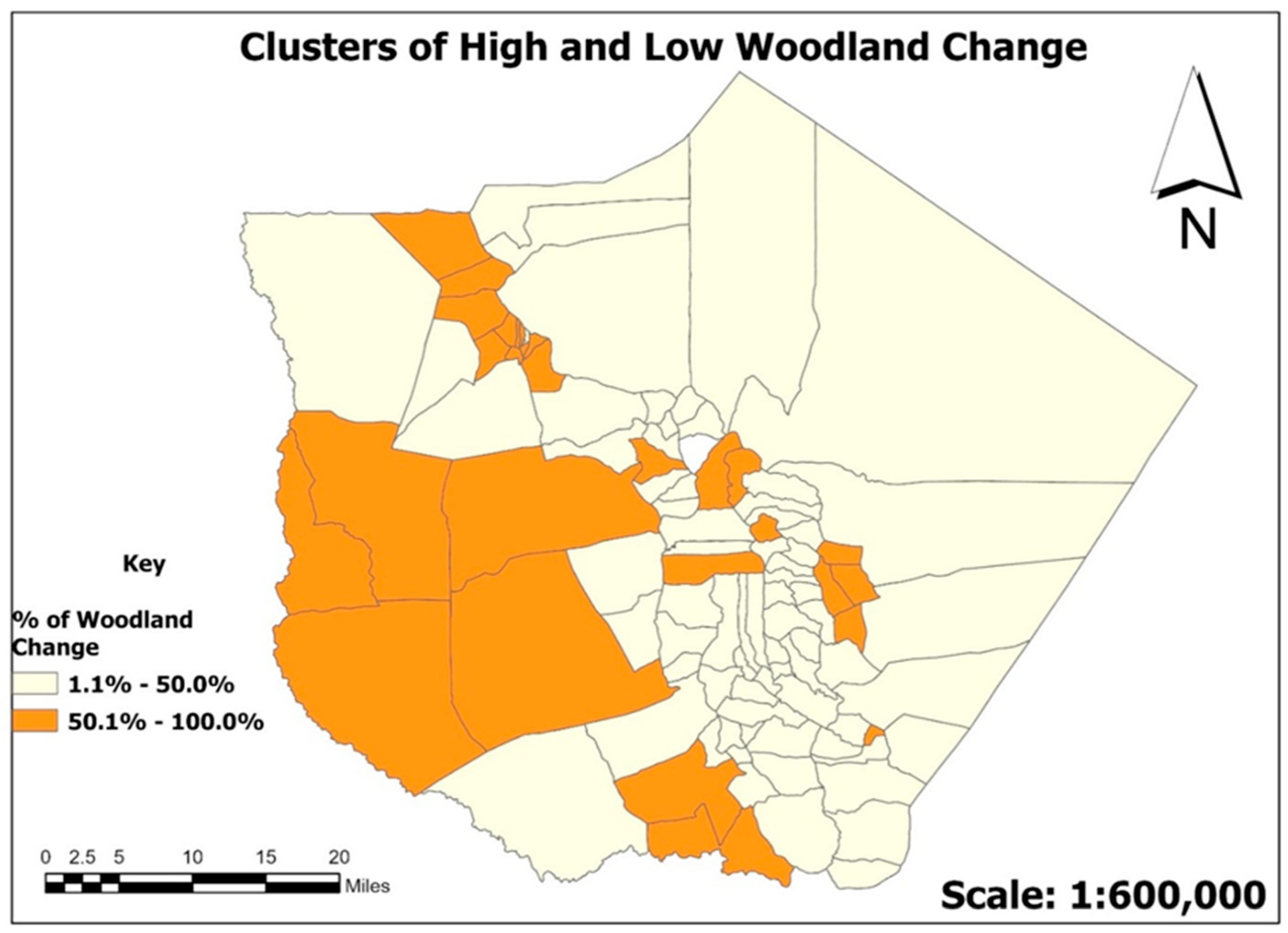
Because this study is focused on woodland change from 2001 to 2020, we used the change detection results to generate a woodland change map of the study area. To determine which villages had significant or minimal woodland change, we utilized ArcGIS Pro’s (v3.0.3). Zonal statistics tool to create a table that linked the woodland change to each of the study area’s 101 villages. This procedure produced statistical values for each village’s woodland change, which were then used to create a study map that displayed the areas with low and significant woodland change. We employed graduated color and symbology in this process, using manual intervals of 50.1–100 (high woodland change) and 0–50 (low woodland change). These thresholds were based on simple binary categorization to distinguish between partial and dominant woodland conversion within each spatial unit, which allows easier visual interpretation and communication of areas with significant change intensity.
The attribute table was also exported to Excel, where we selected one village from a list of a cluster of high woodland change and one village from a cluster of low woodland change using a random sampling technique. Data collection from household surveys is planned in the two selected villages to enhance the woodland change study in Same District. Although the transition table provides valuable insights into the direction and magnitude of land cover changes, the conversions from one category to another may influence the results by leading to overestimation or underestimation of a particular category if there are classification errors from the individual periods. Although this study assessed classification accuracy using an error matrix and reported overall users’ and producers’ accuracy for each classified map, we did not formally calculate uncertainties in the change detection analysis. We suggest a cautious interpretation of the results, and future work could benefit by formally including miscalculation errors.
4. Discussion
The 2020 Landsat 8 image had an overall accuracy of 90% and a Kappa coefficient of 85%, while the 2001 Landsat 7 ETM image had an overall accuracy of 93% and a Kappa coefficient of 86%. These percentages show that the two images were correctly classified. The closest perfect agreement between the reference data and the classified image is indicated by the Kappa Coefficient, which ranges from 0.81 to 0.99 [
56]. Therefore, the study area’s two classified images displayed the closest perfect agreement with the reference data. Similarly, having overall accuracy of 93% and 90% for Landsat 7 ETM and 2020 Landsat 8 images, respectively, shows that the images were correctly classified because they were above 85%, which is the minimum baseline for overall accuracy that is advised [
57]. Other researchers, however, have questioned the accuracy baseline, claiming that it may be lower or higher because a variety of factors can influence the final accuracy [
58,
59].
The study area saw a high rate of woodland loss between 2001 and 2020, with an annual rate of 2.0%. This rate of change is double that of Tanzania’s woodland loss, which was 0.97% annually between 1990 and 2010 [
60]. Another study by [
6] found that between 1975 and 2000, there was a 43% decrease in woodland, or a 1.7% change per year. The study area has seen unprecedented woodland change over the past 20 years, which suggests that the rate of woodland loss is higher than the average for Tanzania. This study showed that although the woodland cover changed, so did other land covers, including cropland, forest, and other land covers like built-up areas and bare land. Earlier research on the Eastern Arc Mountains also showed changes in cropland, forest, and settlement [
6]. The Ref. [
6] study showed that between 1975 and 2000, 5% of the evergreen forest, or closed canopy, which is primarily protected by the government, was lost. These results imply that more research is necessary to identify the factors causing deforestation in the protected forest.
The study revealed that a small portion of the water category was transformed into cropland and other land uses, perhaps because of human activities that have put more strain on the resource. Additionally, as agricultural activities and built-up areas grew, most likely because of an increase in population, a significant portion of the study area’s woodland and forest areas were converted to cropland and other land covers, including settlement. Other studies, such as [
61], demonstrate that the primary cause of land cover change in Tanzania’s Eastern Arc Mountains is agricultural expansion. However, agricultural expansion is not limited to the Eastern Arc Mountains region; according to [
11], agriculture was identified as the primary cause of land cover change in Tanzania as a whole. Demographic factors associated with the effects of population growth that increased the pressures on natural resources, such as woodland and forest resources, are another factor influencing land cover change in Tanzania [
62].
The findings of this study showed that, between 2001 and 2020, the woodland cover lost over 2589.0 km2, or 37.4%, of its land area. However, only a few villages showed a consistent rate of woodland change. This indicates that while some villages in the Same District showed a low loss of woodland, others showed a significant change in woodland above the average. For instance, 71 villages have a change rate of 1% (48.9%), whereas 28 villages have a change rate greater than 50.7% (100%). In this instance, an area was deemed to have a low woodland loss if the change rate was less than 50.7%, and an area with a change rate greater than 50.7% was deemed to have high woodland loss. These results demonstrate that LULCC is both spatial and temporal, meaning that events that occur in one location cannot occur in another or that events that occur over time cannot occur at other times.
Ref. [
63] reports that only 30% of the original woodland and forest cover remains in the study area, indicating a significant decrease in forest and woodland cover. While many studies that have measured land cover change have always extrapolated the rate of change to a particular study area, our research was able to quantify the change in woodland across all the study area’s villages, because change rates can differ amongst study areas.
Due to the growth of agricultural activities and other land uses and land cover, including the expansion of the built-up area within the study area, the woodland cover of the area has changed. According to a study by [
11], the primary causes of the change in woodland cover were deforestation and agricultural expansion, with small-scale farmers accounting for most of the deforestation. Ref. [
11] argues that agriculture has been a primary driver of deforestation in Tanzania. Some academics contend that while shifting cultivation expansion is the main agricultural practice that has been identified as the main driver of woodland decline in many parts of Sub-Saharan Africa, not all forms of agriculture have contributed to the loss of woodlands [
11]. Despite cropland being the second driver in this study, the first being other land covers, such as barren land and built-up areas, agricultural activities can still be the main cause of deforestation in woodlands because other land covers, such as built-up areas, have many combined classes. Similar findings were reported in a study conducted in Ethiopia, which showed that woodlands had decreased because of intense pressure from other land uses, especially agriculture [
64]. Additionally, it has been suggested that woodfuel, such as firewood and charcoal, contributes to the loss of forests. However, ref. [
11] found that charcoal does not significantly contribute to deforestation.
Cropland and other land covers, including built-up areas, replaced woodland in the study area. Numerous detrimental effects on the environment and the community may result from the conversion of woodland to cropland and other land uses. For instance, a study in Ethiopia found that the change in woodland decreased the amount of organic carbon in the soil [
65]. High rates of species loss and ecosystem services have also been observed in areas with high woodland decline [
66]. The loss of species and ecosystem services, such as woodfuel, food, medicine, timber, carbon storage, and water for a variety of purposes, is linked to the decline of woodland and forest in the Eastern Arc Mountains [
63]. Therefore, any change in land cover in the Eastern Arc Mountains study area may have detrimental effects on livelihoods and ecosystems both locally and globally. This is because the Eastern Arc Mountains are known for their remarkable biological diversity, which includes over 550 plant species and about 100 vertebrate species that are unique to the area [
63].
Land cover change affects ecosystem services and people’s livelihoods, including woodfuel, as has been shown in other studies conducted in the Eastern Arc Mountains [
63].
The loss of the woodland begs the question of whether it has become harder for Same District residents to obtain woodfuel. Woodfuel is becoming scarcer according to other studies on the effects of land cover change in other regions [
67], but most rural households continue to rely on it [
68]. The results of this study also support the idea that access to woodfuel resources may be impacted by the high rate of woodland loss between 2001 and 2020.
5. Conclusions
This study aimed to evaluate the change in woodland cover in the Same District in Tanzania’s Eastern Arc Mountains. We conducted LULCC detection for the entire Same District using remote sensing analysis of Landsat 7 for 2001 and Landsat 8 for 2020. We replaced traditional ground truth points with high-resolution Google Earth imagery, NDVI, and a 30 m global cover to create training sites. The alternative solution provided cost savings while also expanding accessibility and coverage of the study area. This study recognizes two main limitations of high-resolution Google Earth imagery, including temporal inconstancy and the absence of spectral data. To address these limitations, we adopted NDVI, and a global cover designed for Landsat’s 2020 image.
We classified the study area into five classes for both images: water, woodland, forest, cropland, and other land covers. The study revealed an adverse change in forest and woodland: −45.1% and −37.4%, respectively. While the study area experienced a decrease in woodland and forest, at the same time, there was a gain in cropland and other land cover for the last 20 years. This trend indicates that agricultural activities and urban development are central forest and woodland loss drivers in the study area. The forest loss did not end only in unprotected areas; it was also revealed in protected areas, which suggests illegal activities are going on.
The significant loss of woodland experienced between 2001 and 2020 represents an annual rate of 2.0% and 2.4% for woodland and forest loss, respectively, despite the large area of natural forest cover being under protected area. Forest loss in the protected area may be attributed to illegal agriculture expansion and illegal logging, implying that forest protection is ineffective in the area. In addition, the forest loss in protected areas threatens biodiversity and ecosystem services in the Eastern Arc Mountains. The evidenced loss of woodland and other land covers in the Eastern Arch Mountains may limit the community’s access to resources. The loss of forest and woodland covers, which essentially make up what is known as the Eastern Arch Mountains, means the failure to support the local population’s livelihoods.
Our study recommends future research to assess the woodland change and other land covers at different scale resolutions. Our study was only focused on a 30 m resolution for the Same District level, despite the Eastern Arc Mountains covering a vast area of Tanzania and Kenya. The research offers important findings about woodland reduction in the Eastern Arc Mountains. It advanced knowledge of woodland loss dynamics and spatial variability in the Same District from 2001 to 2020. However, these findings require careful interpretation because the study was limited to a small area of the Eastern Arc Mountains and relied solely on one resolution scale. We also suggest that future research assess the impact of the decline of the Eastern Arc Mountains’ resources on the community’s access to the resources. Future research should address the impact of woodland loss on rural community access to energy resources such as woodfuel. The reason is that most rural communities in sub-Saharan Africa still depend on forest resources for their energy access.


