An Enhanced Interval Type-2 Fuzzy C-Means Algorithm for Fuzzy Time Series Forecasting of Vegetation Dynamics: A Case Study from the Aksu Region, Xinjiang, China

Abstract

Accurate prediction of the Normalized Difference Vegetation Index (NDVI) is crucial for regional ecological management and precision decision-making. Existing methodologies often rely on smoothed NDVI data as ground truth, overlooking uncertainties inherent in data acquisition and processing. Fuzzy time series (FTS) prediction models based on the Fuzzy C-Means (FCM) clustering algorithm address some of these uncertainties by enabling soft partitioning through membership functions. However, the method remains limited by its reliance on expert experience in setting fuzzy parameters, which introduces uncertainty in the definition of fuzzy intervals and negatively affects prediction performance. To overcome these limitations, this study enhances the interval type-2 fuzzy clustering time series (IT2-FCM-FTS) model by developing a pixel-level time series forecasting framework, optimizing fuzzy interval divisions, and extending the model from unidimensional to spatial time series forecasting. Experimental results from 2021 to 2023 demonstrate that the proposed model outperforms both the Autoregressive Integrated Moving Average (ARIMA) and conventional FCM-FTS models, achieving the lowest RMSE (0.0624), MAE (0.0437), and SEM (0.000209) in 2021. Predictive analysis indicates a general ecological improvement in the Aksu region (Xinjiang, China), with persistent growth areas comprising 61.12% of the total and persistent decline areas accounting for 2.6%. In conclusion, this study presents an improved fuzzy model for NDVI time series prediction, providing valuable insights into regional desertification prevention and ecological strategy formulation.

1. Introduction

Vegetation, as a primary producer in terrestrial ecosystems, links ecological elements such as soil, hydrology, and the atmosphere. It is a core component of the ecosystem structure and function and plays an irreplaceable role in regional ecological regulation [1]. Dynamic trends in vegetation serve as indicators of ecosystem responses to climate change and anthropogenic influences [2,3] while also providing a scientific basis for monitoring land use changes and evaluating the effectiveness of ecological restoration initiatives [4,5]. Particularly in ecologically fragile arid and semi-arid zones, accurate prediction and analysis of the spatial and temporal evolution patterns of vegetation cover are essential prerequisites for optimizing ecological restoration efforts and developing adaptive land management strategies.

With the rapid advancement of satellite technology, remote sensing has become a key tool for monitoring large geographical areas due to its cost-effectiveness and broad coverage [6]. It plays a vital role in large-scale vegetation monitoring and yield prediction [7,8,9]. The Aksu region, located in the arid zone of northwestern China, receives an average annual precipitation of 75 mm and exhibits extremely low ecological resilience to disturbance. This region exemplifies areas in China where climate change sensitivity and ecological vulnerability are closely interconnected [2]. Over the past five decades, observations have shown that the average temperature in the Aksu region has risen significantly while annual precipitation has declined markedly. These changes have led to the gradual expansion of arid zones, posing a substantial threat to biodiversity conservation [10,11]. In light of these challenges, it is crucial to develop a high-precision vegetation cover prediction model to assess regional ecological security thresholds and guide the formulation of adaptive management strategies.

Compared with traditional ground-based monitoring techniques, remote sensing technology has been widely adopted for monitoring large geographical areas due to its cost-effectiveness and extensive coverage [12,13]. However, the quality of data is constrained by various sources of disturbance. During the data acquisition phase, atmospheric perturbations, such as cloud cover and aerosol scattering, can cause fluctuations in the quality of the NDVI time series data. In the data processing stage, differences in resampling algorithms and missing data interpolation introduce system ambiguity. Furthermore, traditional NDVI prediction models typically treat preprocessed data as “real values” and model them directly, ignoring the inherent ambiguity characteristics of the data [14,15]. This may compromise the robustness of the predictive outcomes in the presence of noise-induced disturbances.

Currently, the prediction of vegetation dynamics based on time series remote sensing data can be broadly divided into two categories: deterministic and fuzzy mathematical models. Deterministic models include classical statistical methods such as Markov chains and ARIMA [16,17,18,19], which are computationally efficient and interpretable but often struggle with nonlinear features [20]. Deep learning models such as RNNs and LSTM networks have shown promise in modeling complex nonlinear relationships and have been used in NDVI forecasting [13,15]. However, these models generally require long time series training data and high-performance computational resources, which limit their application in large-scale regions. Additionally, they are sensitive to input data quality and predominantly rely on preprocessed, smoothed NDVI time series data, lacking mechanisms to effectively handle original, non-smooth data. In contrast, machine learning algorithms may offer a more practical alternative for NDVI prediction in large-scale inhomogeneous regions, as they provide stronger computational efficiency and better adaptability while maintaining acceptable prediction accuracy [12].

In recent years, fuzzy algorithms have attracted attention because of their unique advantage in handling outliers, as they can significantly reduce the influence of outliers on the overall inference results by quantifying the degree to which data points belong to a fuzzy set using an affiliation function [21,22,23]. In particular, ref. [24] demonstrated FTS’s effectiveness in forecasting noisy, weakly structured vegetation index time series. Although early studies established the theoretical basis for fuzzy time series (FTS) modeling, they often lacked interpretability in domain partitioning. Subsequent researchers addressed subinterval optimization by introducing clustering algorithms, among which the FCM-FTS algorithm has been widely adopted due to its ability to make subinterval division more interpretable through the use of cluster centers [24,25]. The FCM-based FTS model developed from this framework has been successfully applied in financial forecasting [26], energy system analysis [26], and industrial fault diagnosis [27]. However, its fuzzy coefficient m in the core algorithm is typically set based on the researcher’s experience, leading to unstable subinterval delineation and reduced prediction accuracy. To address this shortcoming, the IT2-FCM method was proposed [28], which mitigates the impact of parameter uncertainty by constructing an interval for the fuzzy coefficient m, and has been shown to achieve more desirable cluster centers than the Type-1 FCM in the presence of data noise [29,30]. Ref. [31] combined IT2-FCM with FTS to forecast time series characterized by high volatility and uncertainty, demonstrating superior performance across four publicly available datasets. However, the IT2-FCM-FTS algorithm, designed for univariate time series, struggles to handle remote sensing time series data, which limits its application in this field.

To address the above problems, this study proposes an improved IT2-FCM-FTS algorithm, which uses the IT2-FCM algorithm for fuzzy interval delineation, extending it from simple time series prediction to a spatiotemporal synergistic prediction framework. Based on the Google Earth Engine (GEE) platform, MOD13Q1 NDVI data from 2001 to 2023 in Aksu were obtained. NDVI data from 2001 to 2020 were used to build a model, which was then used to predict the NDVI for 2021–2023. Product data from the same period were used to validate the model’s accuracy. The improved IT2-FCM algorithm was further applied to predict NDVI in the region from 2024 to 2027 and to analyze vegetation change trends. The findings elucidate long-term spatiotemporal patterns of vegetation change in the Aksu region from 2001 to 2026, offering robust scientific support for adaptive land use planning, systematic ecosystem monitoring, and data-driven environmental policymaking. By introducing an enhanced framework for forecasting remote sensing time series, this study contributes a methodological advancement that facilitates more rigorous, informed, and sustainable approaches to terrestrial ecosystem management.

2. Materials

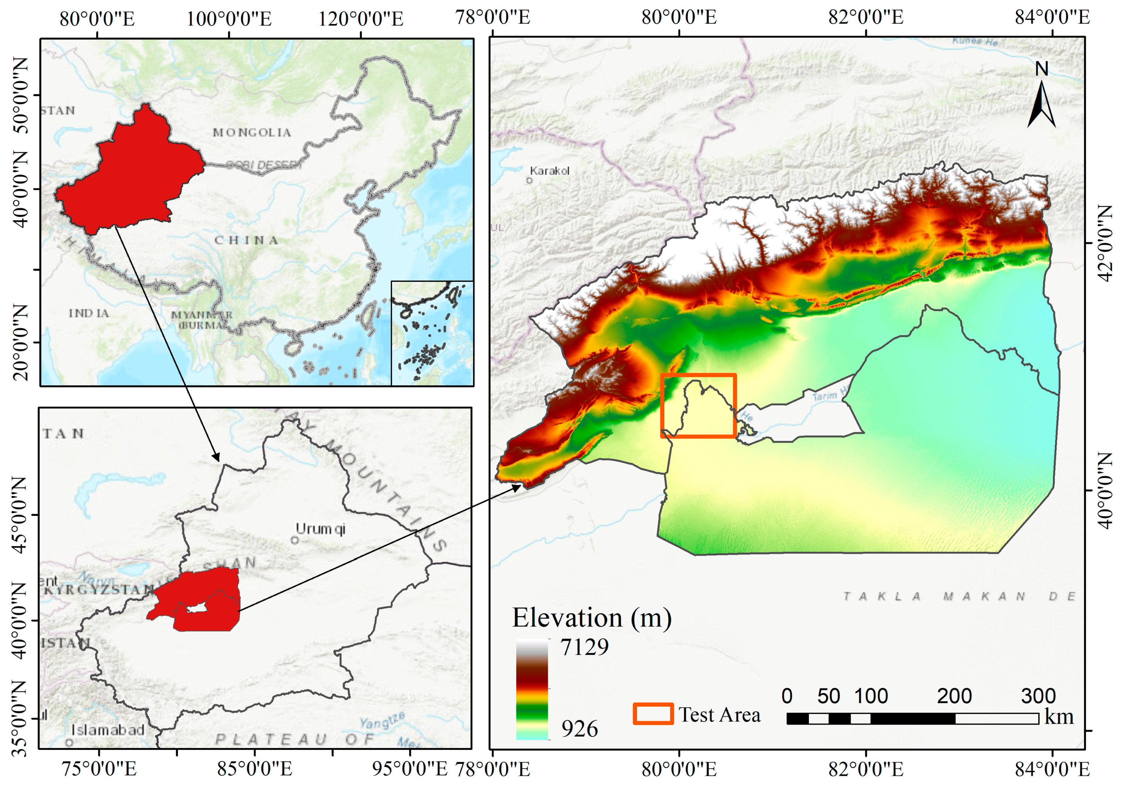
2.1. Study Area

The Xinjiang Uygur Autonomous Region is located in northwestern China, with the Aksu Region situated in its central part. It is bordered by Bayin’guoleng Mongol Autonomous Prefecture to the east, Kizilsu and Kizilsu Kyrgyz Autonomous Prefectures to the west, Hotan Region to the south, and Yili and Kazakh Autonomous Prefectures to the north (Figure 1). The total area of the Aksu Region is approximately 1.32 × 106 km², accounting for 8% of Xinjiang. The topography follows a north-to-south gradient of high mountains, plains, oases, and desert transition zones, with terrain that is elevated in the north and lower in the south, sloping from northwest to southeast. The northern part contains many mountain peaks, while the central region features gravelly fan-shaped foothill zones, alluvial plains, and Gobi areas interspersed with oases. The middle and low hill belts include large areas of well-watered natural grassland characterized by flat terrain, abundant water, and fertile land. The region lies within the arid zone of northwest China and is characterized by dryness and low rainfall, long periods of sunshine, annual sunshine duration of 2750–3029 h, and total solar radiation ranging from 5340 to 6220 MJ/m². Winters are dry and cold, while summers are dry and hot.

2.2. Satellite Data

The MODIS MOD13Q1 NDVI dataset provided by NASA was used in this study, covering the period from 2001 to 2023. This dataset is derived from observations collected by the MODIS sensor aboard the Terra satellite and offers a spatial resolution of 250 m and a temporal resolution of 16 days. It includes information on the NDVI, Enhanced Vegetation Index (EVI), and Quality Assessment (QA) bands. The QA band was utilized for quality assessment. The dataset was preprocessed with geometric, radiometric, and atmospheric corrections and further processed using the Maximum Value Composite (MVC) method to minimize the effects of clouds, atmospheric interference, solar altitude angle, and other factors. Detailed product specifications and data processing methods are available in NASA’s official documentation [32].

2.3. Satellite Data Sources

GEE (https://earthengine.google.com/, accessed on 15 August 2024) is a petabyte-scale platform designed for the scientific analysis and visualization of geospatial data. It provides users with a programmable interface that facilitates efficient large-scale data processing [33]. The MOD13Q1 dataset was retrieved from the GEE platform to extract the NDVI bands for the study area and to harmonize the projection types. Data acquisition was carried out in 16-day intervals, resulting in 23 time points per year and producing 23 independent time series datasets.

2.4. Land Use Data

The land use dataset for the Aksu region employed in this study is primarily derived from Landsat TM/ETM+/OLI remote sensing imagery. After undergoing preprocessing steps such as image fusion, geometric correction, enhancement, and mosaicking, the dataset was produced through a semi-automated visual interpretation approach. Land use types across China were classified into six primary (Level I) categories, twenty-five secondary (Level II) categories, and a limited number of tertiary (Level III) subcategories, ensuring high classification accuracy and spatiotemporal consistency. This study utilized land use data from the year 2020, with a spatial resolution of 250 m (Level I). The data were obtained from the Geographical Information Monitoring Cloud Platform (http://www.dsac.cn/, accessed on 25 May 2025).

3. Methods

This section presents the operational framework of the IT2-FCM-FTS algorithm through a case study involving univariate time series data.

3.1. Sequential Stages in Fuzzy Time Series Implementation

The implementation of the FTS algorithm involves four sequential stages:

(1)

Partitioning the universe based on the sample data.

(2)

Constructing fuzzy sets and applying fuzzification to the time series.

(3)

Extracting fuzzy relationships from the fuzzified sequence and establishing the fuzzy relationship matrix.

(4)

Predicting future values based on the fuzzy relationship matrix obtained in Step (3) and defuzzifying the prediction results.

3.2. Modeling NDVI Time Series Using the IT2-FCM-FTS Approach

Building upon the foundational FTS work of Song and Chissom [21,22], we develop an enhanced forecasting system through the strategic integration of IT2-FCM clustering. The IT2-FCM-FTS framework is subsequently described following a four-step implementation protocol.

3.2.1. Universe Partitioning of NDVI Data Based on IT2-FCM

Utilizing the IT2-FCM clustering algorithm, the thesis universe is determined and partitioned based on the sample data.

According to the sample data, the domain universe $U=\left(D_{min},D_{max}\right)$ is divided into k subintervals $(\mathrm{i}.\mathrm{e}.,U={(u}_1,u_2,\dots ,u_k))$.

The steps for IT2-FCM to delineate the clustering center are as follows:

(1)

Parameter setting: Define two fuzzy parameters, $m_{min},m_{max}$ and assign the maximum and minimum values of m, respectively. $k$ is the number of clusters, and the objective threshold of the objective function $J_m$ is ε. The number of iterations is $t$.

$$J_m=\sum _{i=1}^N\sum _{j=1}^C{u}_{ij}^m{‖x_i-c_j‖}^2,1\le m\le \mathrm{\infty }.$$

(1)

(2)

Initialize the clustering center $C^{\left(t\right)}$.

(3)

Calculate or update the fuzzy interval upper ${u̿}_{i,k}^{\left(t\right)}$, lower ${\overline{u}}^{\left(t\right)}$ interval matrices according to Equations (2) and (3).

$${\stackrel{̿}{u}}_{i,k}^{\left(t\right)}=\left\{\begin{array}{cc}{\displaystyle \frac{1}{{{\sum }_{ik}^k\left(\frac{d_{il}^{\left(t\right)}}{d_{ij}^{\left(t\right)}}\right)}^{\frac{2}{m_{min}-1}}}}& {\displaystyle \frac{1}{{\sum }_{j=1}^k\left(\frac{d_{il}^{\left(t\right)}}{d_{ij}^{\left(t\right)}}\right)}}<{\displaystyle \frac{1}{k}}\\ {\displaystyle \frac{1}{{{\sum }_{ik}^k\left(\frac{d_{il}^{\left(t\right)}}{d_{ij}^{\left(t\right)}}\right)}^{\frac{2}{m_{max}-1}}}}& otherwise\end{array}\right.$$

(2)

$${\overline{u}}_{i,k}^{\left(t\right)}=\left\{\begin{array}{cc}{\displaystyle \frac{1}{{{\sum }_{ik}^k\left(\frac{d_{il}^{\left(t\right)}}{d_{ij}^{\left(t\right)}}\right)}^{\frac{2}{m_{max}-1}}}}& {\displaystyle \frac{1}{{\sum }_{j=1}^k\left(\frac{d_{il}^{\left(t\right)}}{d_{ij}^{\left(t\right)}}\right)}}<{\displaystyle \frac{1}{k}}\\ {\displaystyle \frac{1}{{{\sum }_{ik}^k\left(\frac{d_{il}^{\left(t\right)}}{d_{ij}^{\left(t\right)}}\right)}^{\frac{2}{m_{min}-1}}}}& otherwise\end{array}\right.$$

(3)

where l and $j$ are class labels, ${u̿}_{i,k}^{\left(t\right)}$ and ${\overline{u}}_{i,k}^{\left(t\right)}$ denote the maximum and minimum extents to which $x_i$ belongs to subinterval $u_k$ respectively, and $d_{il}^{\left(t\right)}$, $d_{ij}^{\left(t\right)}$ denote the distance between $x_i$ and $C^{\left(t+1\right)}$.

We then update the cluster center $C^{\left(t+1\right)}$, where the upper and lower fuzzy partition matrices of IT2-FCM are iteratively updated to determine the cluster centers for the interval values, expressed as $[C_L,C_R]$, where $C_L$ and $C_R$ represent the minimum and maximum values of the cluster centers, respectively. The computational formulas are provided in Equations (4) and (5). To ensure $C_L$, when $x_i$ < $C^{\left(t\right)}$ attains its minimum value, the corresponding membership degree is assigned as ${u̿}_{i,k}^{\left(t\right)}$; otherwise, for the maximum value of C_R, the membership degree is ${\overline{u}}_{i,k}^{\left(t\right)}$.

$$C_L=\left\{\begin{array}{c}{\displaystyle \frac{{\sum }_{i=1}^n{x}_i{\stackrel{̿}{u}}_{i,k}}{\sum _{i=1}^n{\stackrel{̿}{u}}_{i,k}}}\hspace{1em}{x}_i<c^{\left(t\right)}\\ {\displaystyle \frac{\sum _{i=1}^n{x}_i{\overline{u}}_{i,k}}{{\sum }_{i=1}^n{\overline{u}}_{i,k}}}\hspace{1em}{x}_i\ge c^{\left(t\right)}\end{array}\right.$$

(4)

$$C_R=\left\{\begin{array}{c}{\displaystyle \frac{\sum _{i=1}^n{x}_i{\overline{u}}_{i,k}}{{\sum }_{i=1}^n{\overline{u}}_{i,k}}}\hspace{1em}{x}_i<c^{\left(t\right)}\\ {\displaystyle \frac{{\sum }_{i=1}^n{x}_i{\stackrel{̿}{u}}_{i,k}}{\sum _{i=1}^n{\stackrel{̿}{u}}_{i,k}}}\hspace{1em}{x}_i\ge c^{\left(t\right)}\end{array}\right.$$

(5)

where $i$ is the index of the time series data, $k$ denotes the subinterval index, and ${u̿}_{i,k}$ and ${\overline{u}}_{i,k}$ represent the maximum and minimum membership degrees for the $i$th sample in the kth subinterval, respectively.

Defuzzification: $C^{\left(t+1\right)}={\displaystyle \frac{\left(C_L+C_R\right)}{2}},$ where $C=\left(C_1,C_2,\dots ,C_K\right)$.

(4)

When $\left|\right|C^{\left(t+1\right)}-C^{\left(t\right)}\left|\right|<\epsilon \to \mathrm{\infty }$, or $t$ reaches the preset value, the iteration stops; otherwise, go back to Step (3) with t = t + 1.

(5)

To derive the final clustering assignments, the IT2 fuzzy partition matrix is first reduced to a type-1 fuzzy set through an averaging operation between its lower and upper membership matrices, i.e., $U={\displaystyle \frac{\left({\overline{u}}^{\left(t\right)}+{\stackrel{̿}{u}}^{\left(t\right)}\right)}{2}}$. The clustering results are subsequently determined by applying the maximum defuzzification criterion.

For each subinterval, its boundary value $dₕ$ (where h = 1, 2,…,$k$) is defined according to the following expression:

$$\left\{\begin{array}{c}{d}_1={\displaystyle \frac{\left(C_1+C_2\right)}{2}}\\ ⋮\\ d_h={\displaystyle \frac{\left(C_h+C_{h+1}\right)}{2}}\\ ⋮\\ d_{k-1}={\displaystyle \frac{\left(C_{k-1}+C_k\right)}{2}}\end{array}\right.$$

(6)

The formula for the subinterval $u_k$ is as follows:

$$\left\{\begin{array}{c}{u}_1=\left(D_{min},d_1\right)\\ u_2=\left(d_1,d_2\right)\\ ⋮\\ u_k=\left(d_{k-1},D_{max}\right)\end{array}\right.$$

(7)

3.2.2. Construction of Interval Type-2 Fuzzy Sets for NDVI Representation

Consider $n$ data samples $x_i,(i=1,2,3,\dots ..,n)$, with fuzzy membership degrees that are evaluated through fuzzification. The degree of affiliation for each subinterval is calculated using the following equation:

$$\left\{\begin{array}{c}{\mu }_{i,1}={\displaystyle \frac{d_1-D_{min}}{\left|x_i-D_{min}\right|+\left|d_1-x_i\right|}}\\ ⋮\\ {\mu }_{i,h}={\displaystyle \frac{d_h-d_{h-1}}{\left|x_i-d_{h-1}\right|+\left|d_h-x_i\right|}}\\ ⋮\\ {\mu }_{i,k}={\displaystyle \frac{D_{max}-d_{k-1}}{\left|x_i-d_{k-1}\right|+\left|D_{max}-x_i\right|}}\end{array}\right.$$

(8)

where ${\mu }_{i,k}$ denotes the affiliation of the $i$th sample data to the kth subinterval.

The fuzzy set $A_i$ is defined as follows:

$$A_i={\displaystyle \frac{{\mu }_{i,1}}{u_1}}+{\displaystyle \frac{{\mu }_{i,2}}{u_2}}+\cdots +{\displaystyle \frac{{\mu }_{i,k}}{u_k}}$$

(9)

3.2.3. Relationship Modeling

The first ($r-1$) data samples are used as the training set to predict the $r$th data point, and the first (r − 1) data samples are fuzzified as a standard matrix.

$$F_r=f_{r-1}=\left[{\mu }_{r-1,1}\hspace{1em}{\mu }_{r-1,2}\hspace{1em}{\mu }_{r-1,3}\hspace{1em}\dots \hspace{1em}{\mu }_{r-1,k}\right]$$

(10)

where ${\mu }_{r-1,k}$ denotes the affiliation value of the first ($r-1$) sample data associated with the kth subinterval, and ${0\le \mu }_{k,r-1}\le 1$.

The first $r-2$ sample data are fused into a computational matrix:

$${B_r^{r-2}=\left(f_1,f_2,f_3\cdots f_{r-2}\right)}^T$$

(11)

The temporal fuzzy relationships within the time series are characterized by a fuzzy relational matrix $R_r$, defined as follows:

$$R_r=F_r·B_r^{r-2}=\left[\begin{array}{ccc}{r}_{1,1}& \cdots & r_{1,k}\\ ⋮& \ddots & ⋮\\ r_{r-\mathrm{2,1}}& \cdots & r_{r-2,k}\end{array}\right]$$

(12)

The fuzzy relationship is constructed using the above equation, and the adjustment term $f_r$ for the$r$th prediction is calculated using the following equation:

$$f_r=\left[\begin{array}{c}max\left(r_{1,1},r_{2,1},r_{r-1,1}\right)max\left(r_{1,2},r_{2,2},r_{r-1,2}\right)\cdots \\ max\left(r_{1,k},r_{2,k},r_{r-1,k}\right)\end{array}\right]=\left[f_{r,1}{f}_{r,2}\cdots f_{r,c}\right]$$

(13)

3.2.4. Defuzzification and Prediction of Future NDVI Values

The predicted change value $f_r$ is defuzzified using the center-of-gravity method to calculate the individual equations as follows:

$$f_r={\displaystyle \frac{{\sum }_{k=1}^k{C}_i{f}_{r,k}}{{\sum }_{k=1}^k{f}_{r,k}}}$$

(14)

where $f\left(r\right)$ is the observation of the $r-1$st sample data, $C_i$ denotes the clustering center, and $f_{r,k}$ denotes the affiliation of the $r$th sample data to the kth clustering center.

3.3. IT2-FCM-FTS Model Parameter Settings

In terms of parameter configuration, based on the previous research results of [34], the fuzzy parameter interval in the IT2-FCM algorithm was set to [m_min, m_max] = [1.8, 2.2], effectively balancing the flexibility of the affiliation function and the algorithm’s stability. The number of clusters k was set to five, following vegetation type classification criteria.

3.4. Evaluation Indices for Prediction Accuracy

To assess the predictive capability of the improved IT2-FCM-FTS algorithm, we established a comprehensive evaluation framework based on three key metrics: the Root Mean Square Error (RMSE), the Standard Error of the Mean (SEM), and the Mean Absolute Error (MAE). The forecasting performance of the IT2-FCM-FTS model was quantitatively compared with those of traditional ARIMA and classical FCM-FTS models through meticulously designed experiments. This comparison elucidates the performance differences among these models, providing valuable insights into their relative effectiveness for time series forecasting tasks.

$$RMSE=\sqrt{{\displaystyle \frac{{\sum }_{i=1}^N{\left(X_i-{\widehat{X}}_i\right)}^2}{N}}}$$

(15)

$$SEM=\sqrt{{\displaystyle \frac{1}{N\left(N-1\right)}}}\sum _{i=1}^N{\left(X_i-{\overline{X}}_i\right)}^2$$

(16)

$$MAE={\displaystyle \frac{1}{N}}\left|X_i-{\widehat{X}}_i\right|$$

(17)

where$N$ denotes the total number of samples, $i$ is the sample ordinal number $0\le i\le N$, $X_i$ denotes the sample true value, ${\widehat{X}}_i$ denotes the sample predicted value, and ${\overline{X}}_i$ denotes the sample mean value.

4. Results

4.1. Model Evaluation

To systematically verify the effectiveness of the improved algorithm, a typical area with high vegetation cover in Aksu was selected as the model validation area (Figure 1). In terms of data partitioning, the NDVI time series data from 2001 to 2020 were used as the training set, while the most recent observation data from 2021 to 2023 were used as the independent validation set to ensure the objectivity of the model assessment. Three algorithms—IT2-FCM-FTS, FCM-FTS, and ARIMA—were used to predict the NDVI for 2021–2023 within the validation area. To comprehensively assess model performance, the average values of the three indicators (RMSE, SEM, and MAE) were calculated separately as quantitative evaluation criteria for model prediction accuracy.

According to the comparative results of the prediction performance shown in

Table 1. Comparative evaluation of NDVI prediction models (2021–2023): RMSE, MAE, and SEM for IT2-FCM-FTS, FCM-FTS, and ARIMA.

Assessment	Model	RMSE	SEM	MAE
Year 2021	ARIMA	0.0654	0.000227	0.0446
	FCM-FTS	0.0788	0.000253	0.0545
	IT2-FCM-FTS	0.0624	0.000209	0.0437
	ARIMA	0.0704	0.000235	0.0489
Year 2022	FCM-FTS	0.0777	0.000248	0.0553
	IT2-FCM-FTS	0.0683	0.000220	0.0489
Year 2023	ARIMA	0.0741	0.000258	0.0513
	FCM-FTS	0.0792	0.000265	0.0556
	IT2-FCM-FTS	0.0724	0.000242	0.0513

, the IT2-FCM-FTS model shows significant advantages in the prediction assessment at the following three time points: its RMSE, SEM, and MAE are the lowest compared with the ARIMA and FCM-FTS models, indicating that the model’s prediction results have a smaller average deviation from the real values and that the degree of dispersion of the multiple prediction results is low, demonstrating a high degree of stability. This demonstrates the feasibility of the improved IT2-FCM-FTS model for time series NDVI plot data prediction and its superiority over the FCM-FTS and ARIMA algorithms. Figure A1 displays partial prediction outcomes, focusing on August during the period from 2024 to 2026.

4.2. NDVI Trend Analysis in the Aksu Region

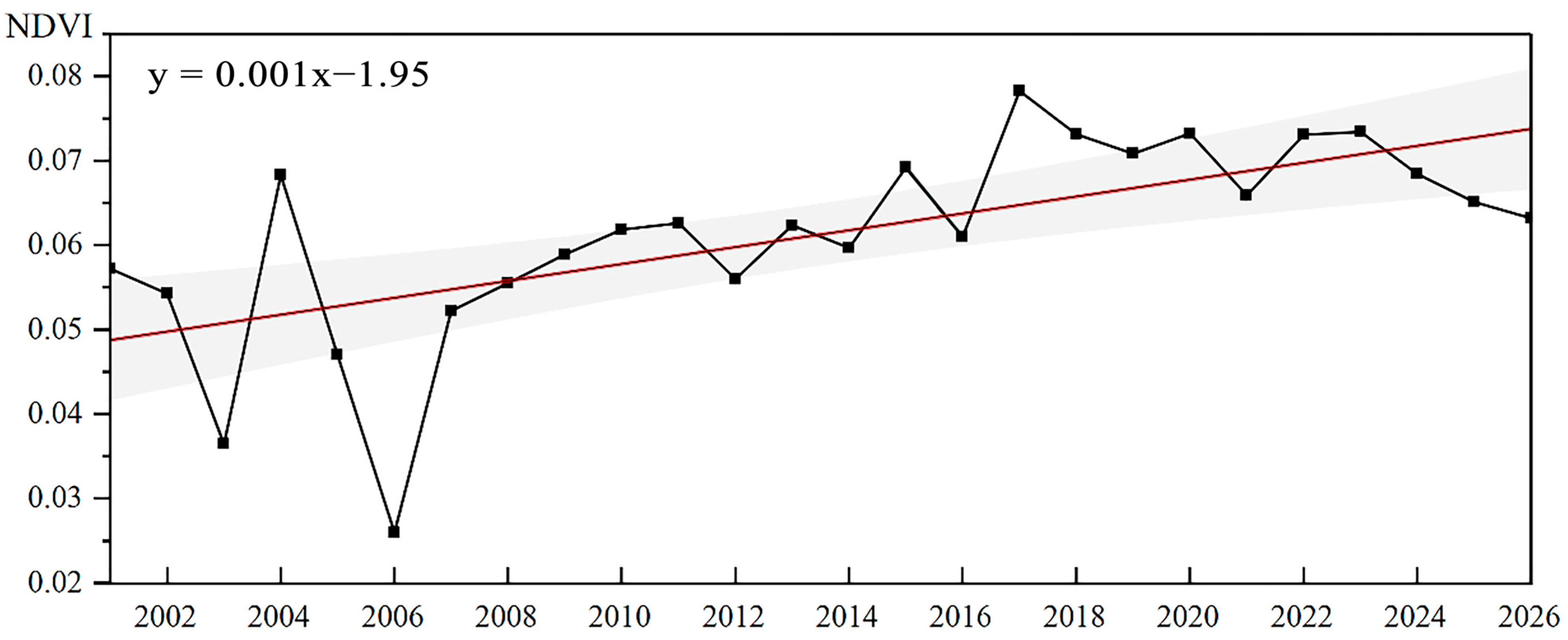
4.2.1. Interannual NDVI Dynamics at the Regional Scale

The overall upward trend in the interannual variation in the mean NDVI in Aksu from 2001 to August 2026 suggests that the surface vegetation cover may have entered a stable expansion phase (Figure 2). This ecologically positive trend may have contributed to enhancing the ecological barrier function of the desert–oasis transition zone. However, the trends in vegetation change, as indicated by NDVI, show considerable spatial heterogeneity (Figure 3). The most significant vegetation increase was observed in Kuqa City and Xinhe County in the northeastern part of the study area. Aksu City showed the next most significant increase, while Keping and Shaya County experienced the weakest growth. All counties demonstrated a significantly increasing trend (p < 0.05).

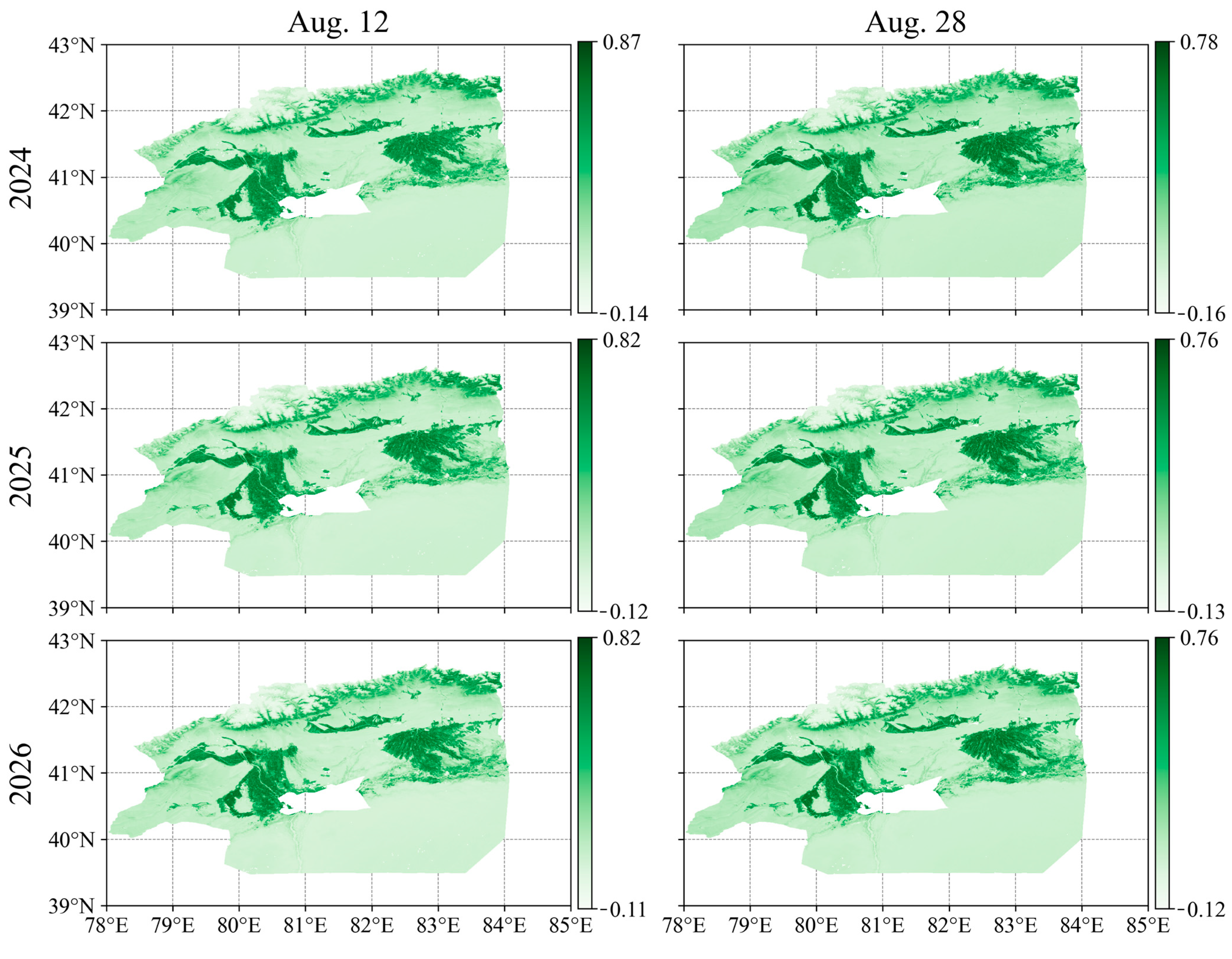
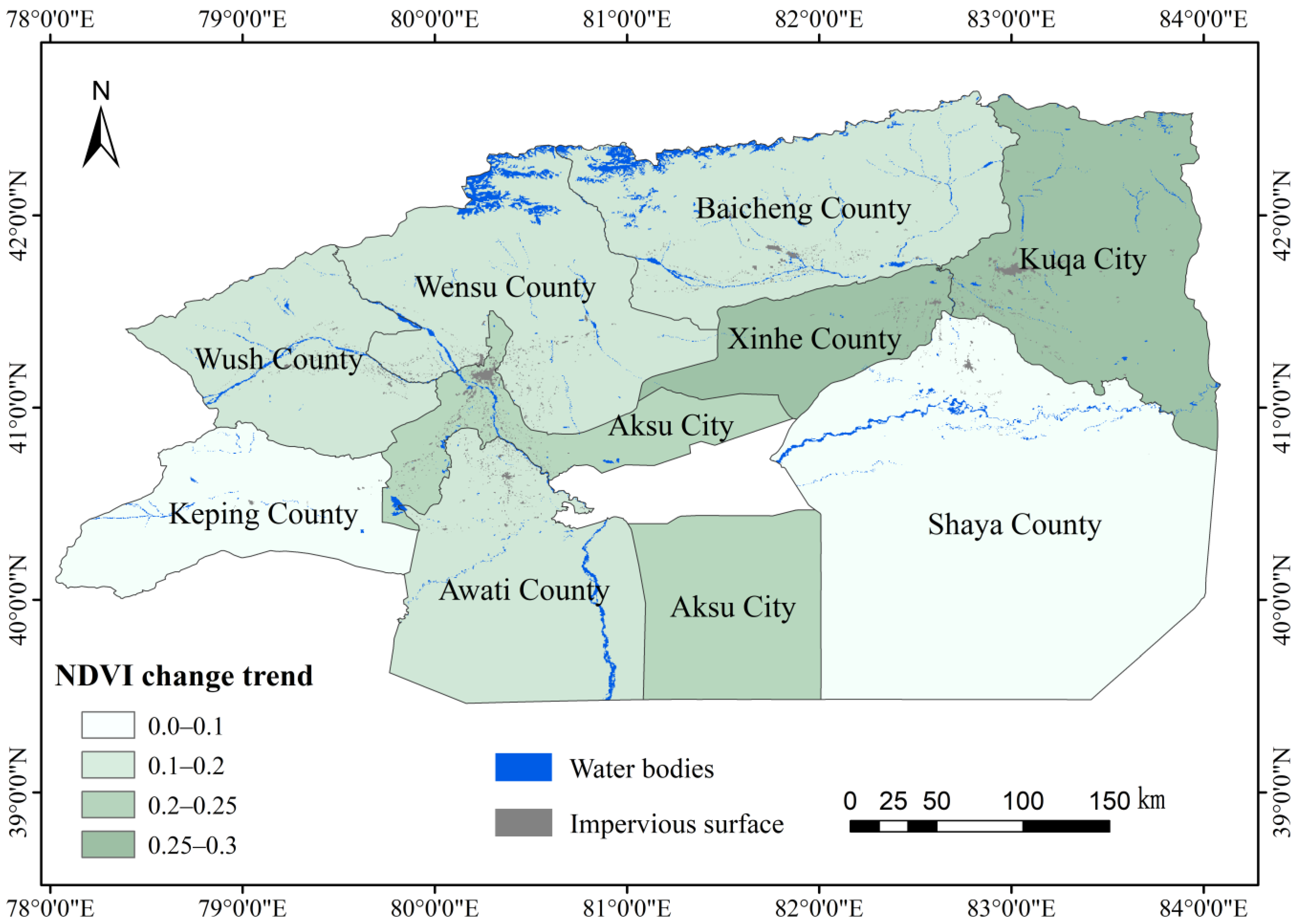
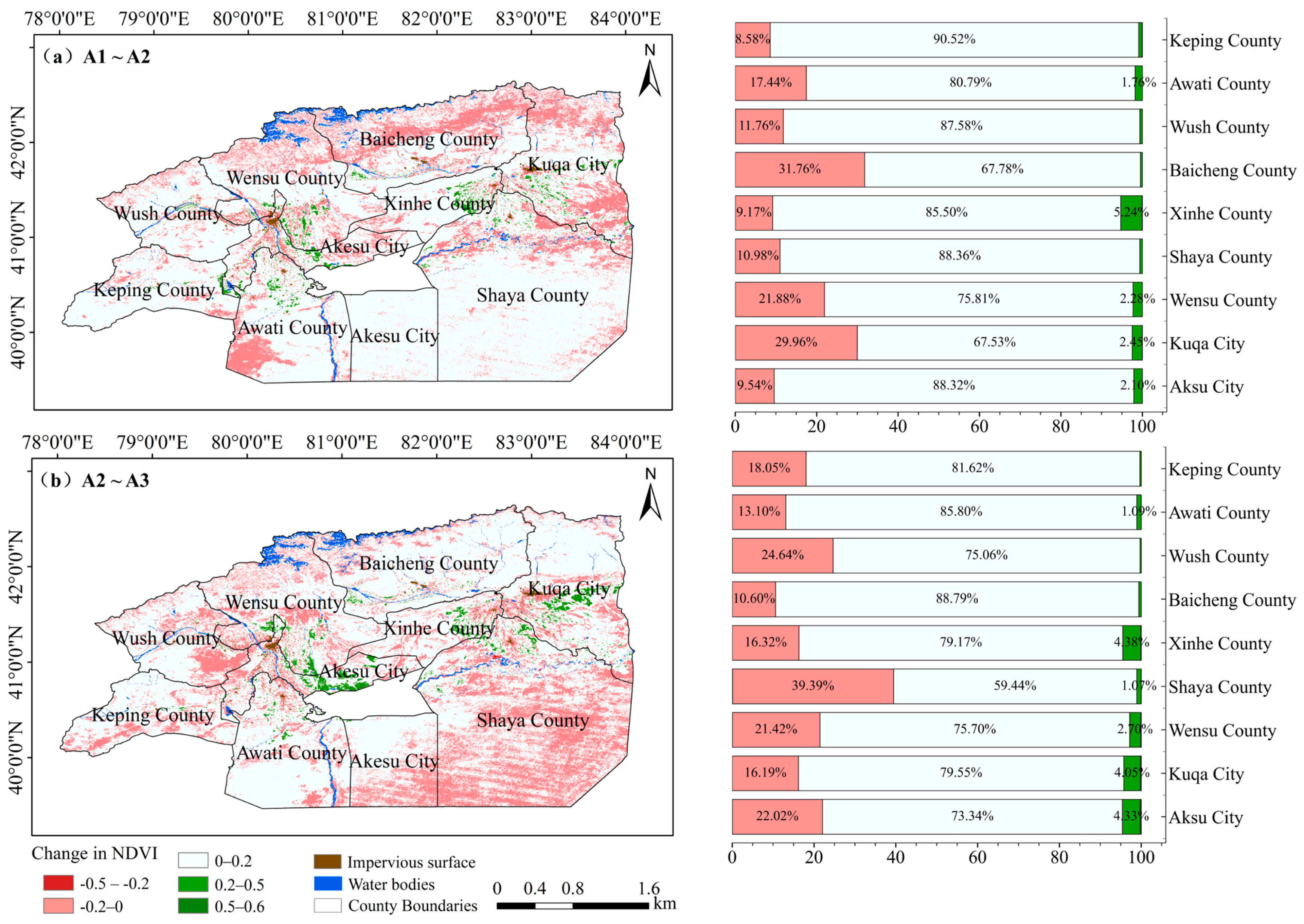
4.2.2. Temporal and Spatial Characteristics of Vegetation Dynamics at the Pixel Scale

This study analyzes the spatiotemporal dynamics of vegetation in the Aksu region by dividing the period from 2001 to 2026 into three stages: 2001–2009 (A1), 2010–2018 (A2), and 2019–2026 (A3). We determined the spatiotemporal characteristics of vegetation condition from the first to the second stage and from the second to the third stage. From the first to the second stage (A1–A2) (Figure 4a), a decrease in NDVI was observed in 17.24% of the total valid land pixels in the Aksu region, with valid pixels defined as those excluding water bodies and impervious surfaces. These decreases were primarily located in northern Baicheng County, northern and southern Kuqa City, southwestern Awati County, and along riverbanks in Shaya County. Larger areas showed a more significant increase, mainly located in eastern Xinhe County, eastern Aksu City, and the junction of Wenxu and Awati Counties. From the second to the third stage (A2–A3) (Figure 4b), an increase in NDVI dominated, covering 76.07% of the total valid pixels in the study area. Decreases occurred mainly in Shaya County, southeastern Aksu City, central Kuqa City, and southwestern Awati County. Larger increases were found in northern Aksu City, central Kuqa City, and eastern Xinhe County.

This study examined the NDVI change process across different stages in the Aksu region (Figure 5) by identifying typical change types that affected more than 1% of the area. The predominant NDVI change type was a continuous increase, accounting for 61.12% of the total area. Areas that experienced an increase followed by a decrease accounted for 20.36% of the total valid pixels, while those experiencing a decrease followed by an increase accounted for 14.60%. Areas with a consistent decrease in NDVI were relatively small, representing only 2.6% of the total area. These NDVI change patterns reflect temporal variations in vegetation activity across the study area, providing insights into the dynamics of vegetation cover over the study period. Overall, the results suggest a general trend of vegetation improvement during the study period. In terms of spatial distribution, pixels with a continuous decrease in NDVI were mainly located in Kuqa City, the junction of Shaya County and Xinhe County, and northern Aksu City. The centers of these areas largely coincide with regions characterized by high impervious surface density and increased human activity, suggesting that urban expansion and land use changes may be the primary drivers of the continuous NDVI decline observed in these regions. In contrast, pixels with a continuous increase were more evenly distributed across the region. Pixels that first increased and then decreased were mainly distributed in Shaya County, Koping County, Wush County, Aksu City, and southern Wensu County. Pixels that decreased and then increased were mainly distributed in northern Baicheng County, northern Kuqa City, and southwestern Awati County.

5. Discussion

5.1. Model Performance and Limitations

The improved IT2-FCM-FTS model outperforms traditional ARIMA and FCM-FTS approaches, with the highest predictive accuracy achieved at the initial forecast point (2021). As with many nonlinear time series models, accuracy gradually declines with extended forecast horizons [15,35]. Nevertheless, the model exhibits strong adaptability in managing data uncertainty while maintaining low computational demands, making it suitable for regions with incomplete records or limited computational infrastructure.

Unlike deep learning methods that require extensive training and large datasets [36,37], this model only needs sufficient historical NDVI or similar time series data and avoids complex parameter tuning. This makes it highly flexible for short-term forecasting across different regions and data types. To ensure reliable fuzzy rule extraction and stable clustering performance, the length of the input time series should exceed the number of defined clusters. Short sequences may compromise model robustness and forecast consistency [37].

Despite the improved performance of the IT2-FCM-FTS model in forecasting NDVI time series, several limitations remain that warrant further investigation and refinement. First, the current prediction framework relies solely on historical NDVI data and does not incorporate key climatic drivers such as precipitation and temperature, which may constrain the comprehensiveness and accuracy of vegetation dynamics forecasting. Second, the model is primarily designed for univariate time series and thus faces challenges when applied to multispectral data or fused remote sensing datasets from multiple sources. Future work should focus on optimizing the model architecture to enhance its capacity for handling multi-source, multi-dimensional data, thereby improving its applicability in complex ecological monitoring scenarios.

5.2. Implications for Sustainable Land Management

This study employs the IT2-FCM-FTS model to forecast NDVI trends in the Aksu region from 2024 to 2026. The results offer valuable insights for local policymakers to anticipate vegetation dynamics, thereby providing a scientific basis for formulating adaptive land use planning, implementing systematic ecosystem monitoring, and developing climate-resilient environmental policies.

However, this case study is still constrained by the spatial resolution and temporal continuity of the available datasets. Future research that incorporates higher-resolution and longer-term remote sensing observations could further enhance the model’s ability to support localized and fine-scale ecological management and land use planning, thereby improving its practical utility and policy relevance in regional environmental governance.

6. Conclusions

In this study, we enhanced a fuzzy time series prediction algorithm based on the IT2-FCM to predict future trends in surface vegetation cover in the Aksu region. We employed three evaluation metrics—RMSE, SEM, and MAE—to compare the performance of our model with that of the ARIMA and FCM fuzzy time series prediction models. The analysis yielded the following findings:

(1)

The improved IT2-FCM-FTS algorithm showed better performance in short-term NDVI prediction than ARIMA and FCM-FTS models, achieving the lowest RMSE (0.0624), MAE (0.0437), and SEM (0.000209) in 2021.

(2)

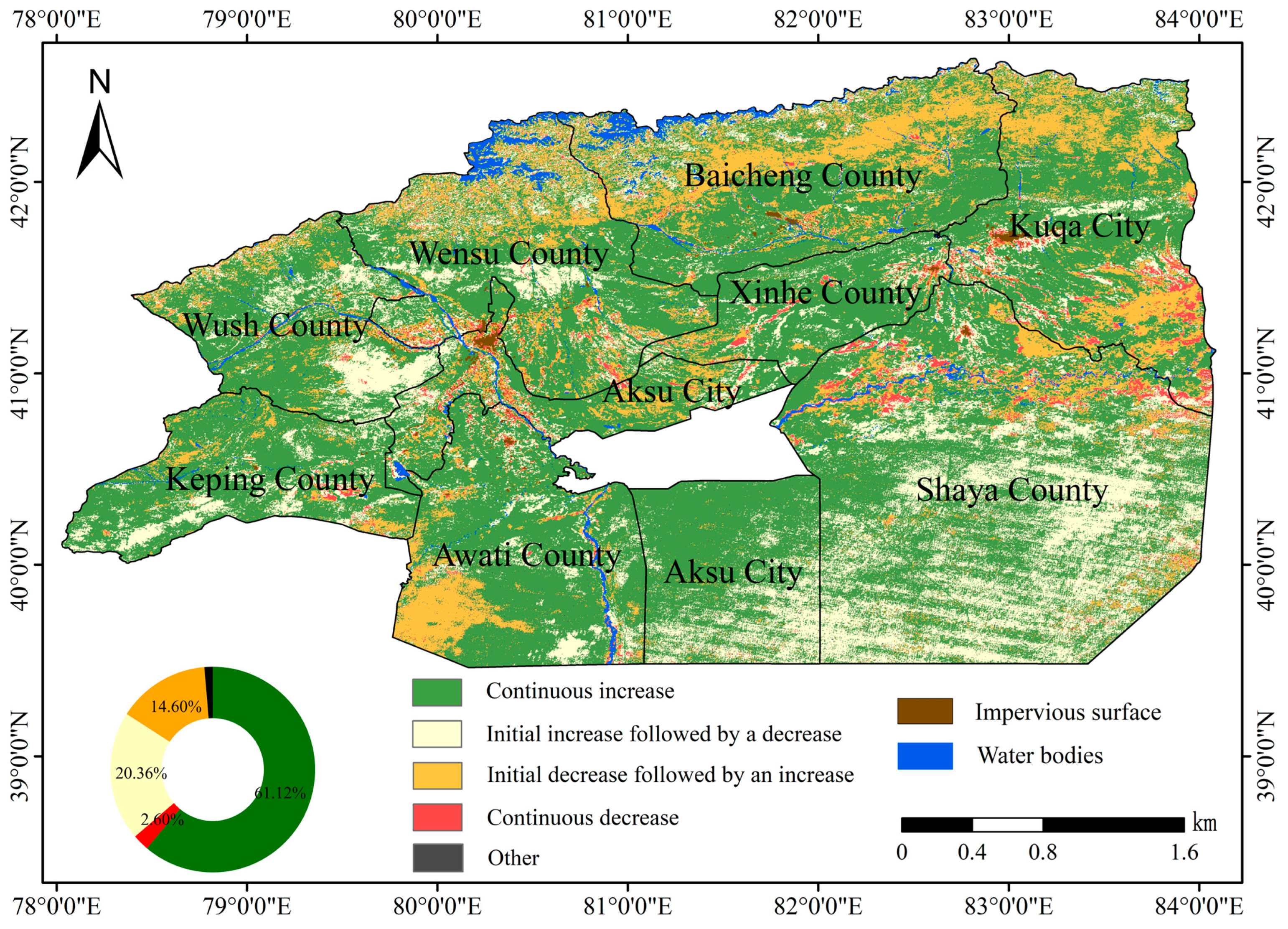
From 2001 to 2026, the NDVI in the Aksu region exhibited a general increasing trend. Notably, areas with a continuous increase accounted for 61.12% of the total area, primarily located in Aksu City, Xinhe County, southern Baicheng County, central Kuqa City, and northern Keping County. Areas with a continuous decrease constituted 2.6% of the total area, mainly along the borders of Kuqa City, Shaya County, Xinhe County, Aksu City, Wensu County, and Wush County.

While this study successfully achieved short-term predictions of NDVI for the Aksu region, it primarily demonstrates the potential of the improved IT2-FCM-FTS model in supporting ecological forecasting in data-limited arid regions. Building on this foundation, future research could explore broader applications of the model in other climate-sensitive areas and examine its integration into long-term sustainability planning and land governance.

References

- Liu, Y.; Li, L.; Chen, X.; Zhang, R.; Yang, J. Temporal-spatial variations and influencing factors of vegetation cover in Xinjiang from 1982 to 2013 based on GIMMS-NDVI3g. Glob. Planet. Chang. 2018, 169, 145–155. [Google Scholar] [CrossRef]
- Alexander, L.; Allen, S.; Bindoff, N.; Breon, F.-M.; Church, J.; Cubasch, U.; Emori, S.; Forster, P.; Friedlingstein, P.; Gillett, N.; et al. Climate Change 2013: The Physical Science Basis.Contribution of Working Group I to the Fifth Assessment Report of the Intergovernmental Panel on Climate Change; Cambridge University Press: Cambridge, UK; New York, NY, USA, 2013. [Google Scholar]
- Zhang, Y.; Ye, A.J.G.; Sensing, R. Quantitatively distinguishing the impact of climate change and human activities on vegetation in mainland China with the improved residual method. GISci. Remote. Sens. 2021, 58, 235–260. [Google Scholar] [CrossRef]
- Kang, L.; Di, L.; Deng, M.; Shao, Y.; Yu, G.; Shrestha, R. Use of geographically weighted regression model for exploring spatial patterns and local factors behind NDVI-precipitation correlation. IEEE J. Sel. Top. Appl. Earth Obs. Remote Sens. 2014, 7, 4530–4538. [Google Scholar] [CrossRef]
- Yang, X.; Liu, S.; Yang, T.; Xu, X.; Kang, C.; Tang, J.; Wei, H.; Ghebrezgabher, M.G.; Li, Z. Spatial-temporal dynamics of desert vegetation and its responses to climatic variations over the last three decades: A case study of Hexi region in Northwest China. J. Arid. Land 2016, 8, 556–568. [Google Scholar] [CrossRef]
- Xue, J.; Su, B. Significant remote sensing vegetation indices: A review of developments and applications. J. Sens. 2017, 2017, 1353691. [Google Scholar] [CrossRef]
- Jaber, S.M. On the relationship between normalized difference vegetation index and land surface temperature: MODIS-based analysis in a semi-arid to arid environment. Geocarto Int. 2021, 36, 1117–1135. [Google Scholar] [CrossRef]
- Piao, S.; Wang, X.; Ciais, P.; Zhu, B.; Wang, T.; Liu, J. Changes in satellite-derived vegetation growth trend in temperate and boreal Eurasia from 1982 to 2006. Glob. Change Biol. 2011, 17, 3228–3239. [Google Scholar] [CrossRef]
- Zheng, K.; Wei, J.-Z.; Pei, J.-Y.; Cheng, H.; Zhang, X.-L.; Huang, F.-Q.; Li, F.-M.; Ye, J.-S. Impacts of climate change and human activities on grassland vegetation variation in the Chinese Loess Plateau. Sci. Total. Environ. 2019, 660, 236–244. [Google Scholar] [CrossRef]
- Wu, Z.; Zhang, H.; Krause, C.M.; Cobb, N.S. Climate change and human activities: A case study in Xinjiang, China. Clim. Chang. 2010, 99, 457–472. [Google Scholar] [CrossRef]
- Xu, C.; Li, J.; Zhao, J.; Gao, S.; Chen, Y. Climate variations in northern Xinjiang of China over the past 50 years under global warming. Quat. Int. 2015, 358, 83–92. [Google Scholar] [CrossRef]
- Farbo, A.; Sarvia, F.; De Petris, S.; Basile, V.; Borgogno-Mondino, E. Forecasting corn NDVI through AI-based approaches using sentinel 2 image time series. ISPRS J. Photogramm. Remote. Sens. 2024, 211, 244–261. [Google Scholar] [CrossRef]
- Stepchenko, A. NDVI index forecasting using a layer recurrent neural network coupled with stepwise regression and the PCA. In Proceedings of the 5th International Virtual Scientific Conference on Informatics and Management Sciences, Shanghai, China, 5–7 November 2016; pp. 130–135. [Google Scholar]
- Reddy, D.S.; Prasad, P.R.C. Prediction of vegetation dynamics using NDVI time series data and LSTM. Model. Earth Syst. Environ. 2018, 4, 409–419. [Google Scholar] [CrossRef]
- Guo, Y.; Zhang, L.; He, Y.; Cao, S.; Li, H.; Ran, L.; Ding, Y.; Filonchyk, M. LSTM time series NDVI prediction method incorporating climate elements: A case study of Yellow River Basin, China. J. Hydrol. 2024, 629, 130518. [Google Scholar] [CrossRef]
- Cui, L.; Zhao, Y.; Liu, J.; Wang, H.; Han, L.; Li, J.; Sun, Z. Vegetation coverage prediction for the Qinling mountains using the CA–Markov model. ISPRS Int. J. Geo-Inf. 2021, 10, 679. [Google Scholar] [CrossRef]
- Darvishi, S.; Solaimani, K. Monitoring and prediction spatiotemporal vegetation changes using NDVI index and CA-Markov model (case study: Kermanshah city). Environ. Sci. 2020, 18, 161–182. [Google Scholar]
- Alhamad, M.; Stuth, J.; Vannucci, M. Biophysical modelling and NDVI time series to project near-term forage supply: Spectral analysis aided by wavelet denoising and ARIMA modelling. Int. J. Remote Sens. 2007, 28, 2513–2548. [Google Scholar] [CrossRef]
- Fernández-Manso, A.; Quintano, C.; Fernández-Manso, O. Forecast of NDVI in coniferous areas using temporal ARIMA analysis and climatic data at a regional scale. Int. J. Remote Sens. 2011, 32, 1595–1617. [Google Scholar] [CrossRef]
- Rhif, M.; Ben Abbes, A.; Martinez, B.; Farah, I.R. A deep learning approach for forecasting non-stationary big remote sensing time series. Arab. J. Geosci. 2020, 13, 1174. [Google Scholar] [CrossRef]
- Ruspini, E.H. A new approach to clustering. Inf. Control 1969, 15, 22–32. [Google Scholar] [CrossRef]
- Song, Q.; Chissom, B.S. Forecasting enrollments with fuzzy time series—Part I. Fuzzy Sets Syst. 1993, 54, 1–9. [Google Scholar] [CrossRef]
- Song, Q.; Chissom, B.S. Forecasting enrollments with fuzzy time series—Part II. Fuzzy Sets Syst. 1994, 62, 1–8. [Google Scholar] [CrossRef]
- Belyakova, P.; Gartsman, B. Possibilities of flood forecasting in the West Caucasian rivers based on FCM model. Water Resour. 2018, 45, 50–58. [Google Scholar] [CrossRef]
- Zhu, L.; Chung, F.-L.; Wang, S. Generalized fuzzy c-means clustering algorithm with improved fuzzy partitions. IEEE Trans. Syst. Man Cybern. Part B (Cybern.) 2009, 39, 578–591. [Google Scholar]
- Rustam, Z.; Vibranti, D.; Widya, D. Predicting the direction of Indonesian stock price movement using support vector machines and fuzzy Kernel C-Means. In AIP Conference Proceedings; AIP Publishing: Melville, NY, USA, 2018. [Google Scholar]
- Salmeron, J.L.; Ruiz-Celma, A.; Mena, A. Learning FCMs with multi-local and balanced memetic algorithms for forecasting industrial drying processes. Neurocomputing 2017, 232, 52–57. [Google Scholar] [CrossRef]
- Rhee, F.C.H.; Cheul, H. A type-2 fuzzy C-means clustering algorithm. In Proceedings of the Proceedings Joint 9th IFSA World Congress and 20th NAFIPS International Conference (Cat. No. 01TH8569), Vancouver, BC, Canada, 25–28 July 2001; Volume 1924, pp. 1926–1929. [Google Scholar]
- Linda, O.; Manic, M. General Type-2 Fuzzy C-Means Algorithm for Uncertain Fuzzy Clustering. IEEE Trans. Fuzzy Syst. 2012, 20, 883–897. [Google Scholar] [CrossRef]
- Sotudian, S.; Zarandi, M.H.F. Interval type-2 enhanced possibilistic fuzzy c-means clustering for gene expression data analysis. arXiv 2021, arXiv:2101.00304. [Google Scholar]
- Yin, Y.; Sheng, Y.; Qin, J. Interval type-2 fuzzy C-means forecasting model for fuzzy time series. Appl. Soft Comput. 2022, 129, 109574. [Google Scholar] [CrossRef]
- Kamel, D.; Munoz, A.; Ramon, S.; Huete, A. MODIS Vegetation Index User’s Guide (MOD13 Series); University of Arizona, Vegetation Index and Phenology Lab: Tucson, AZ, USA, 2015. [Google Scholar]
- Gorelick, N.; Hancher, M.; Dixon, M.; Ilyushchenko, S.; Thau, D.; Moore, R. Google Earth Engine: Planetary-scale geospatial analysis for everyone. Remote Sens. Environ. 2017, 202, 18–27. [Google Scholar] [CrossRef]
- Yuan, F.; Zhan, Y.; Wang, Y. Interval Type-2 Fuzzy c-Means Clustering Method for Interval Data. 2013. Engineering, I. 2013, 34, 1–5. [Google Scholar] [CrossRef]
- Zhu, X.X.; Tuia, D.; Mou, L.; Xia, G.-S.; Zhang, L.; Xu, F.; Fraundorfer, F. Deep learning in remote sensing: A comprehensive review and list of resources. IEEE Geosci. Remote Sens. Mag. 2017, 5, 8–36. [Google Scholar] [CrossRef]
- Shen, L.; Sun, Y.; Yu, Z.; Ding, L.; Tian, X.; Tao, D. On efficient training of large-scale deep learning models: A literature review. arXiv 2023, arXiv:2304.03589. [Google Scholar]
- Khan, A.; Sohail, A.; Zahoora, U.; Qureshi, A.S. A survey of the recent architectures of deep convolutional neural networks. Artif. Intell. Rev. 2020, 53, 5455–5516. [Google Scholar] [CrossRef]