Variation in Soil Organic Carbon and Total Nitrogen Stocks Across Elevation Gradients and Soil Depths in the Mount Kenya East Forest

Abstract

Understanding how elevation gradients and soil depths influence soil organic carbon stocks (SOCS) and total nitrogen stocks (TNS) is essential for sustainable forest management (SFM) and climate change mitigation. This study investigated the effects of elevation and soil depth on SOCS and TNS in the Mount Kenya East Forest (MKEF). A stratified systematic sampling approach was applied, involving collection of 38 soil samples from two depths (0–20 cm and 20–40 cm) across three elevation zones: Lower Forest (1700–2000 m), Middle Forest (2000–2350 m), and Upper Forest (2350–2650 m). Samples were analysed for bulk density (BD), pH, texture, soil organic carbon (SOC), and total nitrogen (TN), using standard laboratory methods. In topsoil (0–20 cm), SOCS ranged from 109.28 ± 23.41 to 151.27 ± 17.61 Mg C ha⁻¹, while TNS varied from 8.89 ± 1.77 to 12.00 ± 2.46 Mg N ha⁻¹. In subsoil (20–40 cm), SOCS ranged from 72.03 ± 19.90 to 132.23 ± 11.80 Mg C ha⁻¹, with TNS varying between 5.71 ± 1.63 and 10.50 ± 1.90 Mg N ha⁻¹. SOCS and TNS increased significantly with elevation (p < 0.05), exhibiting the following trend: Lower Forest < Middle Forest < Upper Forest. Topsoil consistently stored significantly higher SOCS than subsoil (p < 0.05), emphasizing the critical role of surface soils in carbon sequestration. Regression analysis revealed a significant positive relationship between SOCS and TNS (R² = 0.84, p < 0.001). Both SOCS and TNS were positively correlated with elevation, SOC, TN, and total annual precipitation (TAP), but negatively correlated with BD and mean annual temperature (MAT). These findings provide baseline data for monitoring SOCS and TNS in the MKEF, offering insights into sustainable forest management strategies to improve soil health and enhance climate change mitigation efforts.

1. Introduction

Soil organic carbon (SOC) and total nitrogen (TN) are crucial for improving soil quality, supporting vegetation growth, and promoting carbon sequestration [1]. SOC influences key soil physicochemical properties such as structure, cation-exchange capacity (CEC), and water-holding capacity, making it a reliable indicator of soil fertility and health [2]. Additionally, SOC can act as both a source and a sink of atmospheric carbon, influencing climate change [3,4]. Nitrogen, an essential nutrient for plant growth, plays a critical role in the biogeochemical cycling of elements and is a constituent of the Rubisco enzyme, which is vital for photosynthesis [1,5].

SOC and TN contents in a given soil are governed by factors that influence the build-up and removal of soil organic matter (SOM) [6]. As a result, soil organic carbon stocks (SOCS) and total nitrogen stocks (TNS) depend on the balance between carbon inputs from plant productivity and outputs through leaching, decomposition, and erosion [2,7,8]. The SOC pool plays a significant role in the global carbon (C) cycle as minor changes in the SOC pool can translate into large changes in the atmospheric C pool [9]. Thus, soils can either sequester or release atmospheric CO₂, depending on these carbon fluxes [10]. Both SOC and TN fluctuate in response to environmental and human-driven factors [11], with topography, climate, vegetation, parent material, and soil texture acting as environmental influences, while land-use practices and changes play key anthropogenic roles [11,12,13,14,15,16].

Elevation gradient significantly influences SOC by controlling factors such as precipitation, temperature, humidity, solar radiation, and geologic deposition [17,18,19]. Soil depth is another key factor that determines the vertical distribution of SOC in the soil profile as SOC is generally higher in surface horizons than subsurface horizons in most soils due to the regular addition of organic matter from plants and animals [5,20,21]. Tropical montane forests (forests between 23.5° N and 23.5° S with elevations ≥ 1000 m a.s.l) are significant global carbon sinks as they are estimated to store a mean above-ground biomass (AGB) of 271 tonnes per hectare of land surface [22]. Assessing the spatial and vertical distribution of SOC and TN in montane forests is therefore essential to understanding carbon and nitrogen dynamics for sustainable forest management (SFM) [11,23,24].

The MKEF is a critical conservation area in Kenya, renowned for its unique climate, biodiversity, soils, and varied elevation profile [25,26]. It is an important global carbon pool, and is among the five key water towers in Kenya (Mount Kenya forest, Mount Elgon forest, Mau Forest Complex, Cherangany Hills forest, Aberdares forest) that supply ecosystem services and goods to millions of Kenyans [27]. Despite its ecological and environmental significance, the MKEF is under threat from anthropogenic activities and climate change, threatening its ecosystem integrity and potential for climate change mitigation and ecosystem services provision [28]. There is a notable research gap regarding how elevation and soil depth influence SOCS and TNS within this tropical montane ecosystem. Previous studies in the MKEF have primarily focused on forest cover changes and their drivers [29,30,31], vegetation zonation and nomenclature [32], and soil classification [33], with limited comprehensive research on carbon and nitrogen dynamics. This study addresses this gap by investigating the spatial and vertical distribution of SOCS and TNS along different elevation ranges and soil depths in the MKEF. The aim of this study is to (a) quantify variations in SOCS and TNS across different elevation gradients in the MKEF; (b) analyse the distribution of SOCS and TNS across soil depths within various altitudinal zones; and (c) investigate the relationships between SOCS and TNS and selected soil properties and environmental factors in the study area. The present study aligns with some of the United Nations’ Sustainable Development Goals (SDGs), including SDG 13 (climate action) and SDG 15 (life on land), by contributing to climate change mitigation efforts and sustainable land management practices [34]. The research outcomes will contribute to a better understanding of SOC and TN distribution in the MKEF and provide insights for SFM practices and future monitoring. Potential beneficiaries of the findings from this study include forest managers, forest-dependent local communities, and climate change policy makers.

2. Materials and Methods

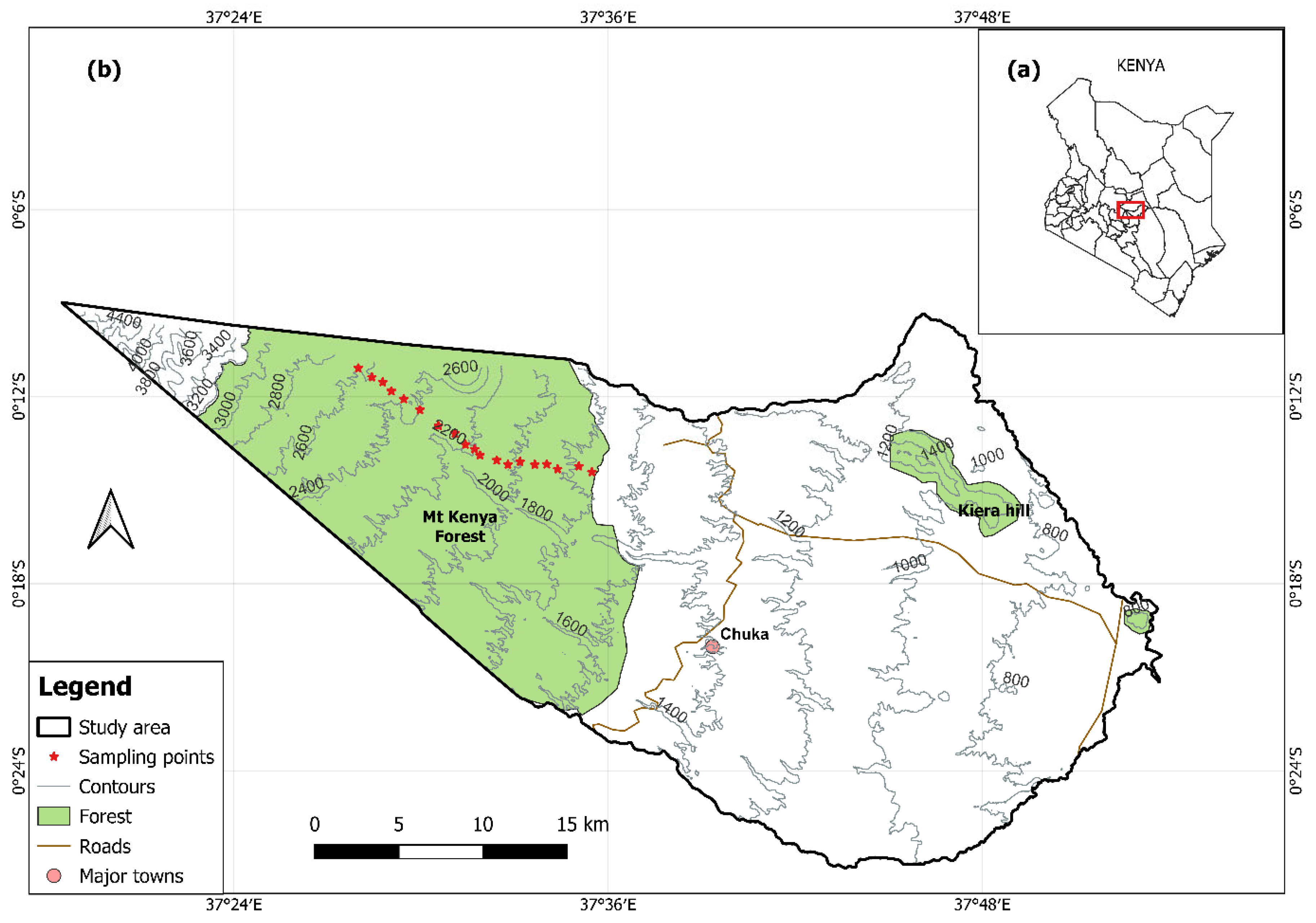
2.1. Study Area

2.1.1. Geographical Location

This study focused on the eastern side of the Mount Kenya Forest, located in Tharaka Nithi County (Figure 1). Geographically, the study area lies between longitudes 37°19′ and 37°46′ east and latitudes 00°07′ and 00°26′ south.

2.1.2. Topography, Geology, and Soils

The study area elevation ranges from 1700 m at the edge of the forest to 5199 m at the peak of Mt. Kenya [35]. This unique altitudinal gradient leads to a varied range of vegetation in a relatively small area, making the region ideal for this kind of study. The geology of the study area is mainly composed of volcanic rocks and ash and some old metamorphic rocks, while the dominant reference soil groups (RSGs) are the humic Andosols [36,37].

2.1.3. Climate

Great altitudinal differences within short distances in the study area lead to great climatic variations over relatively small distances [25]. The MKEF experiences a bimodal rainfall pattern, with total annual precipitation ranging from 1800 mm in the lower forest to 1916 mm in the upper forest (Table 1). The long rains occur from March to June, whereas the short rains are experienced from October to December. The study area’s mean annual temperature ranges from 13.6 °C in the upper forest to 19.2 °C in the lower forest [35].

2.1.4. Water Resources

The Mt. Kenya Forest ecosystem forms a significant water catchment area as it is among Kenya’s five main water towers. It is traversed by several rivers, originating from both Mt. Kenya and the Nyambene Hills, and these form the tributaries of Tana River, which provides water for numerous hydropower stations and domestic users and irrigation schemes [38].

2.1.5. Biodiversity

Vegetation in the sampled locations of the MKEF consists of bamboo forests, indigenous natural montane forests, and plantation forests at different elevations (Table 1). Arundinaria alpine is the dominant bamboo species in the upper forest zone of the MKEF. Some of the common indigenous trees in the forest include camphor (Ocotea usambarensis), podo (Podocarpus latifolius), Meru oak (Vitex keniensis), cedar (Juniperus procera), croton (Croton macrostachyus), wild olive (Olea europaea), and East African rosewood (Hagenia abyssinica). The Eucalyptus spp. is the main exotic plantation tree species in the lower forest zone (Table 1). Animals of conservation interest in the MKEF include African elephant (Loxodonta africana), leopard (Panthera pardus), cape buffalo (Syncerus caffer caffer), bongo (Tragelaphus euryceros), and black-and-white colobus monkey (Colobus guereza). The Mt. Kenya ecosystem is an important bird area (IBA) as it is home to 53 of Kenya’s 67 African highland biome bird species, including the little-known and threatened Abbott’s starling [38,39].

Table 1. General site characteristics of the study area [33,40,41].

Elevation Gradient (m)	Land Use	Vegetation Type	Sampling Locations (n)	Soil Type	Mean Annual Temperature (°C)	Total Annual Rainfall (mm)
2350–2650 (Upper Forest)	Forestland	Natural forest and bamboo thickets - Arundinaria alpine - Podocarpus latifolius - Sambucus africana	6	- Humic Andosols	15.6–13.6	1907–1916
2000–2350 (Middle Forest)	Forestland	Natural forest - Ocotea usambarensis - Podocarpus latifolius - Nuxia congesta - Vitex keniensis - Croton macrostachyus - Olea europaea - Hagenia abyssinica - Sambucus africana	7	- Humic Andosols	18–15.6	1900–1907
1700–2000 (Lower Forest)	Forestland	Natural forest with fragments of plantation forest - Newtonia buchananii - Phoenix reclinate - Eucalyptus spp.	6	- Humic Andosols	19.2–18	1800–1900

Table 1. General site characteristics of the study area [33,40,41].

Elevation Gradient (m)	Land Use	Vegetation Type	Sampling Locations (n)	Soil Type	Mean Annual Temperature (°C)	Total Annual Rainfall (mm)
2350–2650 (Upper Forest)	Forestland	Natural forest and bamboo thickets - Arundinaria alpine - Podocarpus latifolius - Sambucus africana	6	- Humic Andosols	15.6–13.6	1907–1916
2000–2350 (Middle Forest)	Forestland	Natural forest - Ocotea usambarensis - Podocarpus latifolius - Nuxia congesta - Vitex keniensis - Croton macrostachyus - Olea europaea - Hagenia abyssinica - Sambucus africana	7	- Humic Andosols	18–15.6	1900–1907
1700–2000 (Lower Forest)	Forestland	Natural forest with fragments of plantation forest - Newtonia buchananii - Phoenix reclinate - Eucalyptus spp.	6	- Humic Andosols	19.2–18	1800–1900

2.1.6. Demographic and Socio-Economic Characteristics

The study area ethnically consists of the Chuka, Muthambi, Mwimbi, and Tharaka peoples of the larger Ameru community [25,42]. A predominantly farming community surrounds the Mt. Kenya forest reserve [26]. The forest provides several essential ecosystem goods and services, including water, wood, and non-wood forest products, to surrounding communities living within the 5 km forest buffer zone [27,43].

2.2. Sampling Design

A stratified systematic sampling design was adopted for this study, in which sampling locations were distributed based on elevation and vegetation types [44]. Vegetation types formed the strata whereby soil samples were systematically collected at 50 m elevation intervals along a 17 km long and 500 m wide transect. This design was purposefully chosen to ensure that collected soil samples were both representative of the entire study area and provided adequate coverage of the different vegetation strata in the study area. The transect dimensions were selected based on accessibility and safety. The study was conducted within an elevation range of 1700 to 2650 m (Figure 1). The individual elevation points were grouped into three discrete elevation gradient classes for analysis of the effect of altitudinal gradient on SOCS, TNS and other soil properties (Table 1). The three classes were Lower Forest (1700–2000 m), Middle Forest (2000–2350 m), and Upper Forest (2350–2650 m).

2.3. Soil Sampling

The fieldwork was conducted from 25 June to 10 July 2023. The sampling points were pre-determined on Google Earth Pro and mapped in QGIS (3.28.10-Firenze) based on elevation and vegetation types. A handheld GPS device (Garmin E Trex 22x, 2.2”, Garmin Ltd., Olathe, KS, USA) was used to navigate to the designated sampling locations in the field. Soil samples were taken within 20 × 20 m sampling locations from 5 × 5 m sampling plots. Vegetation, debris, litter, stones, and roots were first cleared from the sampling plots; soil samples were then collected using a soil auger (5 cm diameter) at depths of 0–20 cm (topsoil) and 20–40 cm (subsoil). At each sampling plot, samples were taken from four different sub-locations in a Y-shaped pattern [45]. The subsamples were then thoroughly mixed to get a composite sample. A portion of the composite sample was then used to test for the presence of carbonates in the soil using 1 M hydrochloric acid (HCl) [46]. About 500 g of the composite sample was collected from each sampling plot for each depth, bagged in plastic zip loc bags, and labelled. At each sampling location, general site characteristics, including geographical position, vegetation, elevation, and land management practices, were also recorded. A total of 38 disturbed samples were collected using an auger (19 locations × 2 soil depths). Additionally, 38 soil core samples from both depths were separately collected using a 100 cm³ aluminium ring for bulk density (BD) determination [47].

2.4. Preparation and Pre-Treatment of Samples

The core samples were pre-weighed, oven-dried at 105 °C for 24 h, and then re-weighed to obtain the dry weight for BD calculation [47]. The collected soil samples were prepared in Kenya by air-drying, removal of roots by hand, and crushing using a mortar and pestle, followed by sieving through a 2 mm sieve [48]. After the pre-treatment, portions of soil samples (∼200 g) were packed and shipped to the Hungarian University of Agriculture and Life Sciences soils laboratory in Gödöllő, Hungary, for further physicochemical analysis.

2.5. Soil Physicochemical Analysis

Portions of the soil samples were further ground into fine granules using a mortar and pestle and sieved through a 0.25 mm sieve in readiness for SOC and TN analysis. About 5 g of the sieved samples were placed in reusable ceramic crucibles before being analysed for TC and TN by dry combustion using the CNS elemental analyser (Vario MAX cube, Elementar Analysensysteme GmbH, Langenselbold, Germany) [49]. The pH of the soils was measured in a supernatant suspension with a soil-to-liquid ratios of 1:2:5. The liquids were distilled water (pH_H2O) and 1 M Potassium chloride solution (pH KCl); these were and measured with a digital pH meter (VWR pHenomenal pH 1100L, VWR International, Langenselbold, Germany) after the instrument was calibrated with buffer solutions [50]. The soil texture (clay, silt, and sand particles) was determined by the laser diffraction method (LDM) using a laser diffractometer, Mastersizer 3000 (Malvern Instruments, Malvern, UK) as described by [51]. The soil texture classes were subsequently determined using the soil texture classification triangle [52].

2.6. Calculation of Bulk Density, Soil Organic Carbon Stocks, and Total Nitrogen Stocks

The soil BD was calculated as per Equation (1) [53]:

$$\mathrm{BD}={\displaystyle \raisebox{1ex}{$\mathrm{M}\mathrm{s}$}\!\left/ \!\raisebox{-1ex}{$\mathrm{V}\mathrm{s}$}\right.}$$

(1)

where BD—bulk density (g cm⁻³); Ms—mass of dry soil sample (g); Vs—volume of the dry soil sample (cm³)

The SOCS (Mg C ha⁻¹) for each depth was estimated using Equation (2) [54,55,56,57,58]:

SOCS = BD × SOC (%) × d

(2)

where SOCS—soil organic carbon stock (Mg C ha⁻¹); BD—bulk density (g cm⁻³); SOC—soil organic carbon concentration (%); d—sampled soil layer depth (cm).

The TNS (Mg N ha⁻¹) for each depth was estimated using Equation (3) [59]:

TNS = BD × TN (%) × d

(3)

where TNS—total nitrogen stock (Mg N ha⁻¹); BD—bulk density (g cm⁻³); TN—total nitrogen concentration (%); d—sampled soil layer depth (cm).

2.7. Statistical Analysis

A preliminary test for normality among groups was performed on the dataset using the Shapiro–Wilk test before selecting the most suitable statistical analysis. A one-way Analysis of Variance (ANOVA) was used to test for significant differences between the means of the effects of elevation gradient and soil depth using the General Linear Model (GLM). Tukey’s Honestly Significant Difference (HSD) post hoc test was subsequently employed for mean separation purposes. Pairwise comparison tests were also used to assess the mean differences between the two depth levels for different soil properties. The Pearson correlation coefficient and linear regression analysis were utilised to analyse relationships between soil properties and environmental variables. All analyses were performed at a 95% confidence level using R software version 4.2.2 [60] and Microsoft Office Excel 2016.

3. Results

3.1. Selected Soil Physicochemical Properties Within Different Ranges of Elevation Gradients and Soil Depths

Soil pH was lowest in the 0–20 cm depth of the lower forest (4.08 ± 0.23), while the highest pH (5.17 ± 0.54) was recorded in the 20–40 cm depth of the upper forest (

Table 2. Selected soil physicochemical properties under different elevation gradients and soil depths (mean  ±  SD).

Soil Property	Soil Depth (cm)	Elevation Gradient (m)
		1700–2000	2000–2350	2350–2650
BD (g cm−3)	0–20	0.70 ± 0.07 aA	0.63 ± 0.05 aB	0.48 ± 0.05 bB
	20–40	0.75 ± 0.05 aA	0.73 ± 0.07 aA	0.55 ± 0.06 bA
	0–40	0.73 ± 0.06 a	0.68 ± 0.08 a	0.52 ± 0.06 b
SOC (%)	0–20	7.96 ± 2.44 bA	9.31 ± 1.64 bA	15.70 ± 1.74 aA
	20–40	4.77 ± 1.25 bB	6.17 ± 1.02 bB	12.02 ± 1.45 aB
	0–40	6.37 ± 2.49 b	7.74 ± 2.09 b	13.88 ± 2.47 a
TN (%)	0–20	0.65 ± 0.18 bA	0.78 ± 0.13 bA	1.26 ± 0.27 aA
	20–40	0.38 ± 0.10 bB	0.51 ± 0.09 bB	0.94 ± 0.13 aB
	0–40	0.51 ± 0.20 b	0.64 ± 0.18 b	1.10 ± 0.26 a
pH	0–20	4.08 ± 0.23 bA	4.29 ± 0.41 bA	5.02 ± 0.47 aA
	20–40	4.28 ± 0.17 bA	4.26 ± 0.31 bA	5.17 ± 0.54 aA
	0–40	4.18 ± 0.22 b	4.27 ± 0.35 b	5. 09 ± 0.49 a
Sand (%)	0–20	24.98 ± 6.33 bA	35.18 ± 7.44 bA	58.90 ± 20.21 aA
	20–40	10.16 ± 3.99 bB	16.52 ± 5.22 bB	46.38 ± 13.99 aA
	0–40	17.57 ± 9.24 b	25.85 ± 11.48 b	52.64 ± 17.82 a
Silt (%)	0–20	55.42 ± 2.16 aA	51.55 ± 5.73 aA	35.86 ± 16.96 bA
	20–40	56.00 ± 2.64 abA	56.85 ± 3.86 aA	45.74 ± 11.41 bA
	0–40	55.71 ± 2.32 a	54.20 ± 5.44 a	40.80 ± 14.71 b
Clay (%)	0–20	19.61 ± 4.76 aB	13.27 ± 2.47 bB	5.24 ± 3.34 cA
	20–40	33.84 ± 3.40 aA	26.62 ± 5.33 bA	7.89 ± 2.65 cA
	0–40	26.72 ± 8.41 a	19.94 ± 7.99 b	6.56 ± 3.19 c
Texture	0–20	Silt Loam	Silt Loam	Sandy Loam
	20–40	Silty Clay Loam	Silt Loam	Loam
	0–40	Silt Loam	Silt Loam	Sandy Loam

Note: Different lowercase letters indicate significant differences in soil properties between elevation gradients within the same range of soil depth, whereas different uppercase letters indicate significant differences in soil properties between soil depths within the same range of elevation gradient.

). The highest SOC (15.70 ± 1.74%) was present in the topsoil of the 2350–2650 m elevation range, while the lowest SOC (4.77 ± 1.25%) was observed in the subsoil of the 1700–2000 m elevation gradient. The SOC generally decreased with declines in elevation gradient and soil depth. The TN content fluctuated between 0.38 ± 0.10% and 1.26 ± 0.27. TN similarly increased with increasing elevation gradient (Table 2).

The soil BD values varied between 0.48 ± 0.05 g cm⁻³ and 0.75 ± 0.05 g cm⁻³ along the elevation gradients. Significantly higher BD values were noted in the lower forest relative to the upper forest for both soil depths (Table 2). The mean sand contents for the aggregated depth (0–40 cm) ranged from a low of 17.57 ± 9.24% in the lower forest to 52.64 ± 17.82% in the upper forest. Higher sand content was consistently observed at each elevation gradient in topsoil, compared with the subsoil (Table 2). Silt content varied between 35.86 ± 16.96% and 56.85 ± 3.86%. Clay content ranged from a minimum of 6.56 ± 3.19% in the upper forest’s topsoil to a maximum of 33.84 ± 3.40% in the lower forest’s subsoil. Consistently higher clay content was observed in subsoil than in topsoil at each elevation gradient. Soil texture comprised clay loam (1700–2000 m and 2000–2350 m), and sandy loam (2350–2650 m) for the aggregated soil depth (Table 2).

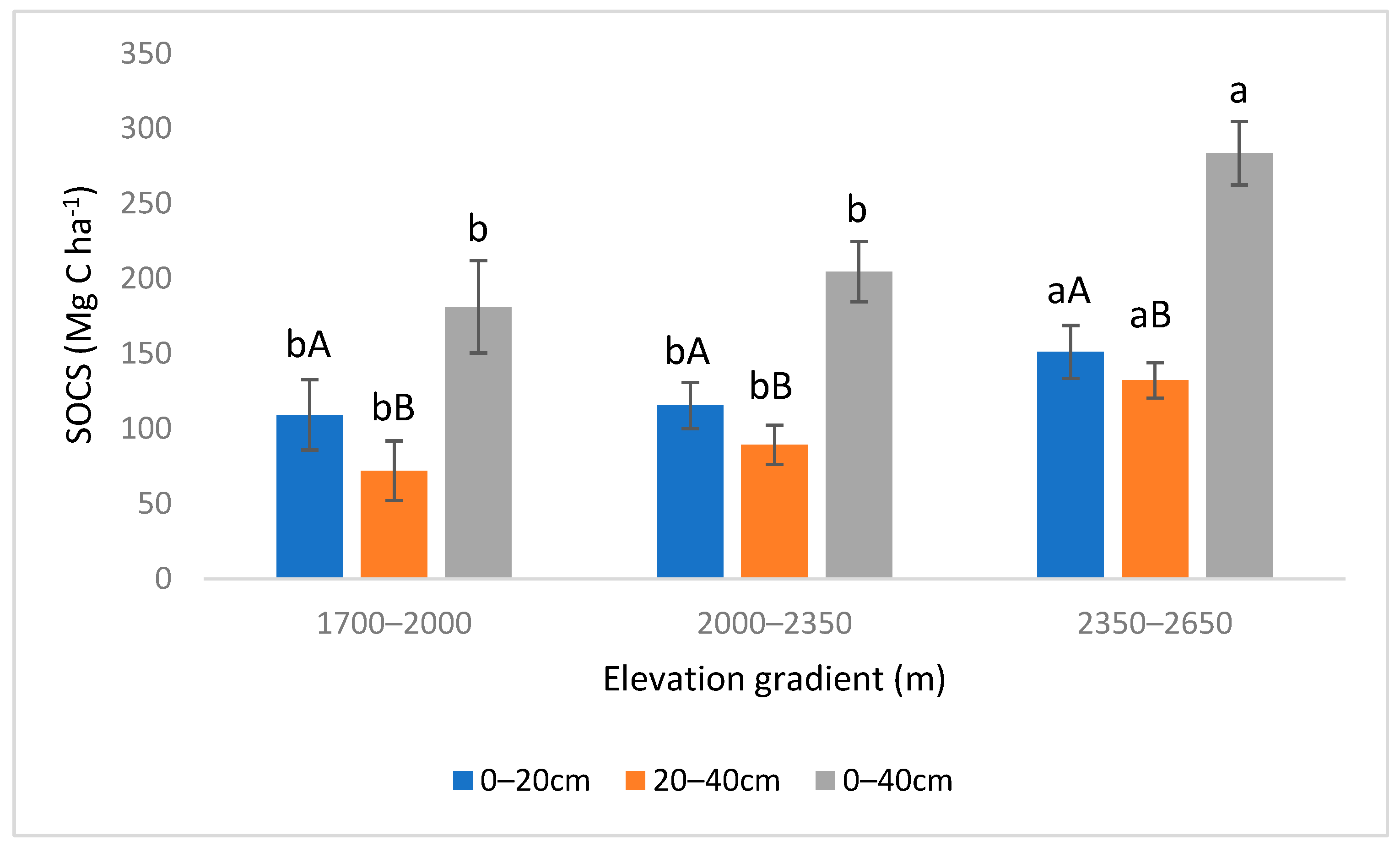
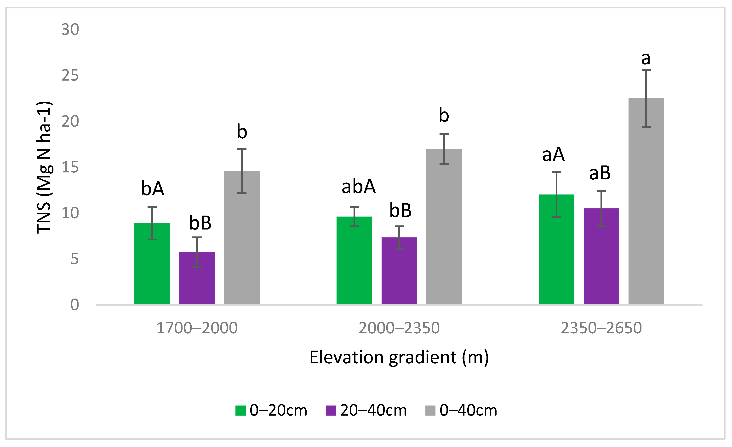
3.2. Variations in SOCS and TNS with Elevation Gradient and Soil Depth

The ANOVA results showed a significant influence of elevation gradient and soil depth on both SOCS and TNS in the study area soils (

Table 3. ANOVA results showing the influence of elevation gradient and soil depth on SOCS and TNS.

Variables	SOCS (Mg C ha−1)				TNS (Mg N ha−1)
	DF	F Value	p-Value	Significance	DF	F Value	p-Value	Significance
Elevation Gradient	2	17.82	4.6 × 10−6	***	2	11.50	0.000145	***
Depth	1	9.429	0.00405	**	1	9.592	0.00378	**

Note: ** and *** indicate significance at 0.01, and 0.001, respectively.

).

The SOCS in the 0–20 cm depth ranged from 109.28 ± 23.41 Mg C ha⁻¹ in the lower forest (1700–2000 m) to 151.27 ± 17.61 Mg C ha⁻¹ in the upper forest (2350–2650 m). For the 20–40 cm layer, SOCS ranged from 72.03 ± 19.90 Mg C ha⁻¹ in the lower forest to 132.23 ± 11.80 Mg C ha⁻¹ in the upper forest. The aggregated SOCS for the 0–40 cm depth ranged from 181.31 ± 30.72 Mg C ha⁻¹ in the 1700–2000 m elevation gradient to 283.50 ± 21.13 Mg C ha⁻¹ in the 2350–2650 m elevation gradient (Figure 2). The mean SOCS based on elevation gradient was in the order of upper forest > middle forest > lower forest for all depths, with the upper forest having significantly higher SOCS than the middle and lower forest (Figure 2). Overall, significantly higher SOCS were recorded in topsoil vis-a-vis subsoil at all three elevation gradients (Figure 2).

Similar change trends were observed for TNS with elevation gradients and soil depths. The mean TNS at 0–20 cm soil depths ranged from 8.89 ± 1.77 to 12.00 ± 2.46 Mg N ha⁻¹ while at 20–40 cm depths, the TNS ranged between 5.71 ± 1.63 to 10.50 ± 1.90 Mg N ha⁻¹ (Figure 3). The aggregated TNS (0–40 cm) ranged from 14.60 ± 2.41 to 22.50 ± 3.10 Mg N ha⁻¹. Significant TNS differences (p < 0.05) were observed between the topsoil and subsoil for each elevation range and between the upper-forest and lower-forest elevation ranges for the respective soil depths. The TNS correspondingly showed a decreasing trend with increasing soil depth and an increasing trend with increasing elevation (Figure 3).

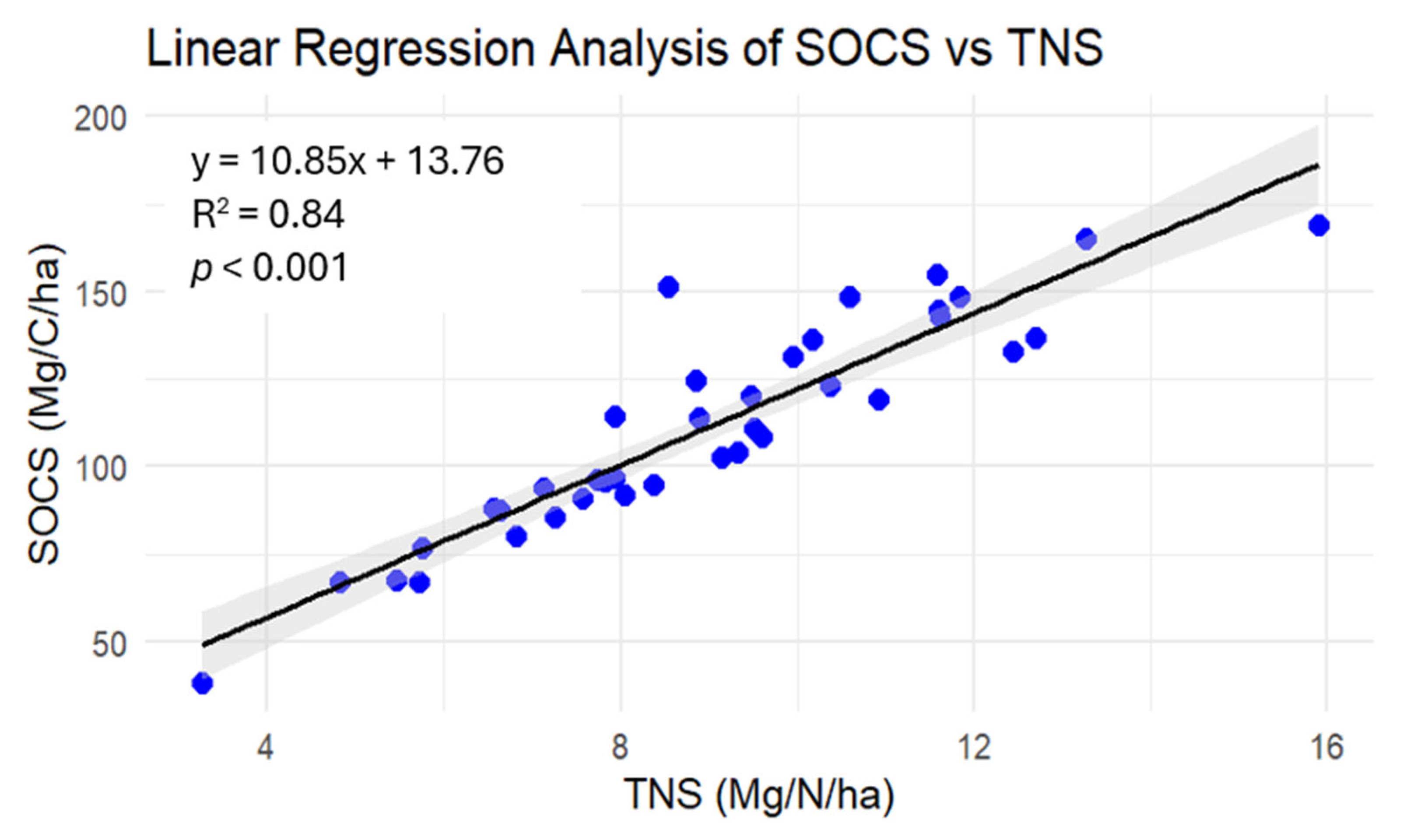
3.3. Relationship Between SOCS and TNS

A linear regression analysis was run to establish the relationship between SOCS and TNS (Figure 4). The regression analysis results showed a significant positive relationship between the SOCS and TNS, indicating that most of the variations in SOCS could be explained by the changes in TNS (R² = 0.84, p < 0.001).

3.4. Correlations Between SOCS and TNS and Other Soil Properties and Environmental Variables

Pearson correlation coefficient analysis was conducted to find out the relationships between SOCS and TNS and environmental variables (TAP, MAT, elevation) and other soil properties (BD, pH, SOC, TN, sand, silt, and clay).

3.4.1. Correlations Between SOCS and TNS and Other Soil Properties

Results from the correlation analysis revealed that SOCS and TNS both exhibited positive significant correlations with SOC, TN, and sand. Conversely, for both SOCS and TNS, negative correlations with BD, silt and clay were observed (Figure 5).

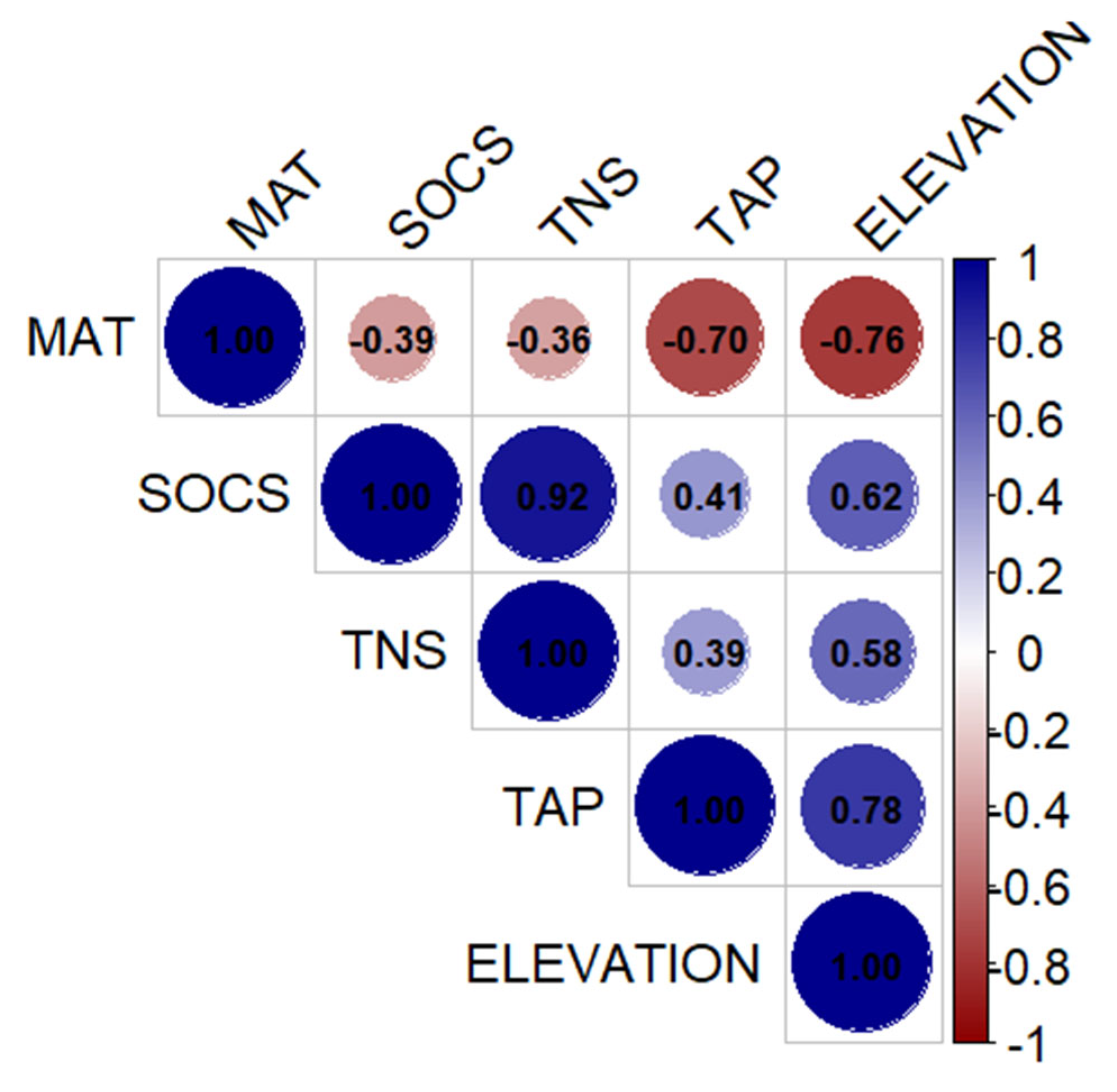
3.4.2. Correlation Between SOCS and TNS and Environmental Variables

As for the environmental variables both the SOCS and TNS were positively correlated with elevation and TAP and negatively correlated with MAT (Figure 6).

4. Discussion

4.1. Overview of Selected Physicochemical Properties of Study Area Soils

Findings from the present study showed variations in selected soil physical and chemical properties along elevation gradients and between soil depths. Significantly lower BD values were recorded in the upper forest and in the topsoil layer of the soil profile. These results corroborate the findings from other studies of similar landscapes [53,61,62]. Lower BD values in the upper forest can be attributed to higher SOM contents and less human disturbance. The high SOM content increases soil volume without significantly affecting its weight, reducing BD proportionally [63]. The increase in BD with incremental soil depth could also be related to decreased SOM content and the compaction pressure of the overlying soil horizons [64]. Other researchers have likewise reported that surface soil layers generally have high SOM content, better particle size distribution, good aggregation, and root penetration, resulting in low BD values [16,65].

The pH of the studied soils was generally acidic (pH < 7.0) in nature. Soils developed from non-calcareous parent materials, typical of our study area, are inherently acidic [66]. The mean forest soil pH in the lower forest was very strongly acidic, whereas the upper forest soils were strongly acidic [67]. The varying pH values in our study can be related to differences in vegetation density and composition, soil moisture, and temperature between the three gradients. Very strongly acidic pH in the lower forest can also be associated with the presence of eucalyptus spp. The leaves and bark of eucalyptus spp. produce acidic litter and allelopathic compounds which contribute to a decrease in soil pH over time [68]. Eucalyptus spp. is also fast-growing and can deplete the soil of base cations (calcium, magnesium, and potassium) that help to buffer soil acidity. This uptake reduces the soil’s ability to neutralize acids, leading to acidification [69].

Higher sand content characterizes the upper elevation range of the forest, relative to the middle and lower elevation ranges. A similar trend was reported for Mount Bambouto, Central Africa [70] and for the Birr watershed, upper Blue Nile Basin, Ethiopia [16]. The observed decrease in sand content with depth could be due to the erosion of smaller size particles such as clay from higher elevations of the forest into the lower elevations, given the topography of the study area. The higher clay content in subsoil, compared with topsoil, at all elevation ranges can be attributed to downward clay translocation [71].

SOC and TN content was lowest in the lower forest and highest in the upper forest, with both showing an increasing trend with increases in elevation gradient. These variations in SOC and TN content are proportional to the quantity of litter accumulated on the soil surface under the different vegetation types and the carbon inputs through plant residue decomposition [72].

4.2. SOCS and TNS Variation with Elevation Gradient and Soil Depth

SOCS and TNS content showed a systematic upward trend with increasing elevation in the MKEF. A characteristic variation in vegetation types was equally observed across altitudinal strata and among sites in the present study. Our results corroborate with findings obtained by other researchers [70,73,74,75], which showed a similar increase in SOCS with increased elevation in tropical montane forest landscapes. Elevation plays a crucial role in the buildup and breakdown of SOC because of its significant impact on various co-varying environmental factors [76]. Specifically, alterations in climate at different elevations shape the composition and primary productivity of vegetation, influencing the amount and turnover of SOM through the regulation of soil water balance, soil erosion, soil temperatures, soil pH, soil texture, and geologic deposition processes [76,77,78,79]. Since SOC is the major source of TN, an increase in SOCS subsequently results in increased TNS [71].

Mean SOCS and TNS values in the lower forest were significantly lower than in the upper forest. In the upper forest, the presence of diverse indigenous vegetation species, a dense canopy, lower MAT due to less exposure to sunlight, and higher TAP jointly contribute to greater SOM accumulation relative to the other elevation gradients [32]. The study exhibited an outstanding differences in altitude within short distances, which leads to great variation in climate and vegetation type over relatively small distances [39]. Lower levels of SOCS in the lower forest may be associated with a lower diversity of vegetation species, as it comprises a mix of natural and plantation forest [32]. The lower forest also exhibited an open canopy as the trees were widely spaced, resulting in lower litter input and less accumulation of SOM. Indications of human disturbances were also observed in the lower forest as it is easily accessible by the communities bordering the forest, in contrast to both the middle and upper forest where human disturbances are rarely reported [39]. Communities bordering the lower forest depend on the forest for their livelihood and often encroach into the forest for charcoal production, firewood collection, illegal timber logging, construction poles, and fodder harvesting [27,38,39,80]. This results in the continuous removal of dead wood, twigs, litter, and trees, hence the lower recorded SOCS content. This finding aligns with those reported in ref. [70] for Mount Bambouto, Central Africa, and in ref. [81] for the Ethiopian Central Highlands, where the accumulation of SOCS in the upper forest was attributed to longer vegetative growing periods with less human interference than in the lower forest, where diminished SOCS was recorded near human settlements. In addition, a study in the Mount Marsabit Forest Reserve, a sub-humid montane forest in northern Kenya, established that SOCS was concentrated in the least disturbed forest areas, while reduced levels of SOCS were observed in disturbed forest areas with pronounced anthropogenic activities [82]. The mid- and upper-elevation zones of the MKEF, which store higher levels of SOC and TNS, should be a focus for adaptive forest management strategies aimed at maintaining and enhancing carbon sequestration. Conservation of natural forests in these zones can significantly contribute to climate change mitigation at the landscape scale.

4.3. Relationships Between SOCS and TNS and Environmental Variables and Other Soil Properties

A significant relationship was observed between SOCS and TNS in the MKEF. This result corroborates with findings by other researchers in similar mountainous regions [73,83,84]. The results suggest that most of the TN variations are related to SOC storage changes, and the accumulation of C could influence TNS [84]. The present study showed that SOCS and TNS were significantly correlated with other soil parameters (SOC, TN, BD, pH, sand, silt, and clay), and environmental variables (MAT, TAP and elevation). This finding underlines the complex relationships and interactions of the soil properties within the soil system and with the environment. The negative correlation of both SOCS and TNS with BD identified in our study is consistent with results of previous studies which also identified a negative relationship between the soil properties [21,78,85]. The inverse relationship between BD and SOCS implies that the lower SOCS typically translates to higher BD as SOC has a very low weight per unit volume [62]. The observed negative correlation between SOCS and MAT in the study area can be linked to the steady increase in soil temperature with reduced elevation. Temperature affects microbial activity and decomposition rates [86]. Lower temperatures result in SOM accumulation because of the slower breakdown of SOM by microorganisms [87]. Increasing temperatures down the elevation gradient contributes to increased SOC loss via decomposition, reducing SOCS [88].

SOCS and TNS both exhibited a significant positive correlation with sand and a negative correlation with clay (Figure 5). This finding is in line with that reported in ref. [70] for a mountainous region of Western Cameroon. Contrary to our results, other studies conducted in similar landscapes have reported a significant positive correlation between SOCS and clay [89,90,91]. These contradicting findings are an indication that the physical and chemical characteristics of soil under similar land uses are not universally consistent but, rather, contingent upon various factors such as soil type, climatic conditions, vegetation types, and management practices [75].

5. Conclusions

This study assessed the effects of elevation gradients and soil depths on SOCS and TNS in the MKEF. The findings demonstrate that elevation significantly influences SOCS and TNS at all depths, with mean values increasing progressively with elevation, reaching peak levels in the upper forest zone (Lower Forest < Middle Forest < Upper Forest). Similarly, SOCS and TNS were consistently higher in the topsoil compared to the subsoil across all elevation gradients, emphasizing the critical role of surface soils in nutrient storage and carbon sequestration.

Regression analysis revealed a strong positive relationship between SOCS and TNS (R² = 0.84, p < 0.001), while correlation analysis highlighted both positive and negative associations with other soil properties and environmental factors, such as BD, TAP, and MAT. These findings underscore the complex interactions between soil properties and environmental conditions, which govern nutrient cycling and carbon dynamics.

The study underscores the MKEF’s vital roles in carbon sequestration and in maintaining high SOCS levels, both of which are critical for soil health and climate change mitigation. The forest serves as a vital ecological reservoir of soil fertility and carbon, offering insight into how elevation, soil depth, and environmental variables influence soil nutrient dynamics. The findings further provide essential baseline data for long-term monitoring of SOCS and TNS in the region, to inform adaptive land-use policies and help align conservation programs with broader sustainable development goals. They also highlight the importance of incorporating elevation and soil depth into forest management strategies. Sustainable forest management (SFM) practices, including the protection and restoration of natural forest vegetation, especially in the lower altitude zones where greater loss of SOC and TNS was observed, are essential for preserving soil health and enhancing the carbon sequestration potential of the MKEF. The findings from the present study also have important implications for surrounding farming communities, as they can guide sustainable agricultural practices in adjacent farmlands, including the use of agroforestry, conservation tillage, and organic soil amendments for improved soil health and climate change mitigation.

References

1. Zhao, Z.; Zhang, X.; Dong, S.; Wu, Y.; Liu, S.; Su, X.; Wang, X.; Zhang, Y.; Tang, L. Soil Organic Carbon and Total Nitrogen Stocks in Alpine Ecosystems of Altun Mountain National Nature Reserve in Dry China. Environ. Monit. Assess. 2019, 191, 1–12. [Google Scholar] [CrossRef] [PubMed]
2. Basile-Doelsch, I.; Chevallier, T.; Dignac, M.-F.; Erktan, A. Carbon Storage in Soils, 2nd ed.; Elsevier Inc.: Amsterdam, The Netherlands, 2023; ISBN 9780128229743. [Google Scholar]
3. Martin, M.P.; Wattenbach, M.; Smith, P.; Meersmans, J.; Jolivet, C.; Boulonne, L.; Arrouays, D. Spatial Distribution of Soil Organic Carbon Stocks in France. Biogeosciences 2011, 8, 1053–1065. [Google Scholar] [CrossRef]
4. Xin, Z.; Qin, Y.; Yu, X. Spatial Variability in Soil Organic Carbon and Its Influencing Factors in a Hilly Watershed of the Loess Plateau, China. Catena 2016, 137, 660–669. [Google Scholar] [CrossRef]
5. Bangroo, S.A.; Najar, G.R.; Rasool, A. Effect of Altitude and Aspect on Soil Organic Carbon and Nitrogen Stocks in the Himalayan Mawer Forest Range. Catena 2017, 158, 63–68. [Google Scholar] [CrossRef]
6. Ahmad Dar, J.; Somaiah, S. Altitudinal Variation of Soil Organic Carbon Stocks in Temperate Forests of Kashmir Himalayas, India. Environ. Monit. Assess. 2015, 187, 1–15. [Google Scholar] [CrossRef] [PubMed]
7. Ontl, T.A.; Schulte, L.A. Soil Carbon Storage. Nat. Educ. Knowl. 2012, 3, 35. [Google Scholar]
8. Lal, R. Challenges and Opportunities in Soil Organic Matter Research. Eur. J. Soil Sci. 2009, 60, 158–169. [Google Scholar] [CrossRef]
9. Lal, R. Beyond COP21: Potential and Challenges of the “4 per Thousand” Initiative. J. Soil Water Conserv. 2016, 71, 20A–25A. [Google Scholar] [CrossRef]
10. Schrumpf, M.; Schulze, E.D.; Kaiser, K.; Schumacher, J. How Accurately Can Soil Organic Carbon Stocks and Stock Changes Be Quantified by Soil Inventories? Biogeosciences 2011, 8, 1193–1212. [Google Scholar] [CrossRef]
11. Stockmann, U.; Adams, M.A.; Crawford, J.W.; Field, D.J.; Henakaarchchi, N.; Jenkins, M.; Minasny, B.; Mcbratney, A.B.; Remy, V.D.; Courcelles, D.; et al. The Knowns, Known Unknowns and Unknowns of Sequestration of Soil Organic Carbon. Agric. Ecosyst. Environ. 2013, 164, 80–99. [Google Scholar] [CrossRef]
12. Post, W.M.; Kwon, K.C. Soil Carbon Sequestration and Land-Use Change: Processes and Potential. Glob. Chang. Biol. 2000, 6, 317–327. [Google Scholar] [CrossRef]
13. Guo, L.B.; Gifford, R.M. Soil Carbon Stocks and Land Use Change: A Meta Analysis. Glob. Chang. Biol. 2002, 8, 345–360. [Google Scholar] [CrossRef]
14. Sun, W.; Zhu, H.; Guo, S. Soil Organic Carbon as a Function of Land Use and Topography on the Loess Plateau of China. Ecol. Eng. 2015, 83, 249–257. [Google Scholar] [CrossRef]
15. Liu, Z.; Shao, M.; Wang, Y. Effect of Environmental Factors on Regional Soil Organic Carbon Stocks across the Loess Plateau Region, China. Agric. Ecosyst. Environ. 2011, 142, 184–194. [Google Scholar] [CrossRef]
16. Amanuel, W.; Yimer, F.; Karltun, E. Soil Organic Carbon Variation in Relation to Land Use Changes: The Case of Birr Watershed, Upper Blue Nile River Basin, Ethiopia. J. Ecol. Environ. 2018, 42, 1–11. [Google Scholar] [CrossRef]
17. Tsui, C.C.; Chen, Z.S.; Hsieh, C.F. Relationships between Soil Properties and Slope Position in a Lowland Rain Forest of Southern Taiwan. Geoderma 2004, 123, 131–142. [Google Scholar] [CrossRef]
18. Tsui, C.C.; Tsai, C.C.; Chen, Z.S. Soil Organic Carbon Stocks in Relation to Elevation Gradients in Volcanic Ash Soils of Taiwan. Geoderma 2013, 209–210, 119–127. [Google Scholar] [CrossRef]
19. Kong, J.; He, Z.; Chen, L.; Zhang, S.; Yang, R.; Du, J. Elevational Variability in and Controls on the Temperature Sensitivity of Soil Organic Matter Decomposition in Alpine Forests. Ecosphere 2022, 13, e4010. [Google Scholar] [CrossRef]
20. Blackburn, K.W.; Libohova, Z.; Adhikari, K.; Kome, C.; Maness, X.; Silman, M.R. Influence of Land Use and Topographic Factors on Soil Organic Carbon Stocks and Their Spatial and Vertical Distribution. Remote Sens. 2022, 14, 2846. [Google Scholar] [CrossRef]
21. Ali, S.; Begum, F.; Hayat, R.; Bohannan, B.J.M. Variation in Soil Organic Carbon Stock in Different Land Uses and Altitudes in Bagrot Valley, Northern Karakoram. Acta Agric. Scand. Sect. B Soil Plant Sci. 2017, 67, 551–561. [Google Scholar] [CrossRef]
22. Spracklen, D.V.; Righelato, R. Tropical Montane Forests Are a Larger than Expected Global Carbon Store. Biogeosciences 2014, 11, 2741–2754. [Google Scholar] [CrossRef]
23. Tashi, S.; Singh, B.; Keitel, C.; Adams, M. Soil Carbon and Nitrogen Stocks in Forests along an Altitudinal Gradient in the Eastern Himalayas and a Meta-Analysis of Global Data. Glob. Chang. Biol. 2016, 22, 2255–2268. [Google Scholar] [CrossRef]
24. Zech, M.; Hörold, C.; Leiber-Sauheitl, K.; Kühnel, A.; Hemp, A.; Zech, W. Buried Black Soils on the Slopes of Mt. Kilimanjaro as a Regional Carbon Storage Hotspot. Catena 2014, 112, 125–130. [Google Scholar] [CrossRef]
25. County Government of Tharaka Nithi. Third County Integrated Development Plan (2023–2027); County Government of Tharaka Nithi: Kathwana, Kenya, 2023. [Google Scholar]
26. Rotich, B.; Maket, I.; Kipkulei, H.; Melenya, C.; Nsima, P.; Ahmed, M.; Csorba, A.; Micheli, E. Determinants of Soil and Water Conservation Practices Adoption by Smallholder Farmers in the Central Highlands of Kenya. Farming Syst. 2024, 2, 100081. [Google Scholar] [CrossRef]
27. Nature Kenya. Ecosystem Service Assessment for the Restoration of Mount Kenya Forest; Nature Kenya: Nairobi, Kenya, 2019. [Google Scholar]
28. Otieno, T.A.; Otieno, L.A.; Rotich, B.; Löhr, K.; Kipkulei, H.K. Modeling Climate Change Impacts and Predicting Future Vulnerability in the Mount Kenya Forest Ecosystem Using Remote Sensing and Machine Learning. Environ. Monit. Assess. 2025, 197, 1–21. [Google Scholar] [CrossRef]
29. Bussmann, R.W. Destruction and Management of Mount Kenya’s Forests. Ambio 1996, 25, 314–317. [Google Scholar]
30. Akotsi, E.F.N.; Ndirangu, J.K.; Gachanja, M. Changes in Forest Cover in Kenya’s Five “Water Towers” 2003–2005; Department of Resource Surveys and Remote Sensing: Nairobi, Kenya, 2006. [Google Scholar]
31. Rotich, B.; Ahmed, A.; Kinyili, B.; Kipkulei, H. Historical and Projected Forest Cover Changes in the Mount Kenya Ecosystem: Implications for Sustainable Forest Management. Environ. Sustain. Indic. 2025, 26, 100628. [Google Scholar] [CrossRef]
32. Bussmann, R.W. Vegetation Zonation and Nomenclature of African Mountains—An Overview. Lyonia 2006, 11, 41–66. [Google Scholar]
33. Muchena, F.N.; Gachene, C.K.K. Soils of the Highland and Mountainous Areas of Kenya with Special Emphasis on Agricultural Soils. Mt. Res. Dev. 1988, 8, 183–191. [Google Scholar] [CrossRef]
34. United Nations. Transforming Our World: The 2030 Agenda for Sustainable Development. Resolution Adopted by the General Assembly on 25 September 2015, 42809, 1–13; United Nations: New York, NY, USA, 2015. [Google Scholar]
35. County Government of Tharaka Nithi. Tharaka Nithi County Integrated Development Plan 2018–2022; County Government of Tharaka Nithi: Kathwana, Kenya, 2018. [Google Scholar]
36. Dijkshoorn, J.A. Soil and Terrain Database for Kenya (Ver. 2.0) (KENSOTER); ISRIC-World Soil Information: Wageningen, The Netherlands, 2007. [Google Scholar]
37. IUSS Working Group WRB. World Reference Base for Soil Resources 2014, Update 2015 International Soil Classification System for Naming Soils and Creating Legends for Soil Maps; World Soil Resources Reports No. 106; FAO: Rome, Italy, 2015. [Google Scholar]
38. Kenya Wildlife Service. Mt. Kenya Ecosystem Management Plan 2010–2020; Kenya Wildlife Service: Nairobi, Kenya, 2010. [Google Scholar]
39. Kenya Forest Service. Mt. Kenya Forest Reserve Management Plan 2010–2019; Kenya Wildlife Service: Nairobi, Kenya, 2010; pp. 4–9. [Google Scholar]
40. Jaetzold, R.; Schmidt, H.; Hornet, Z.B.; Shisanya, C. Farm Management Handbook of Kenya, 2nd ed.; Natural Conditions and Farm Information, Volume 11/C; Eastern Province, Ministry of Agriculture/GTZ: Nairobi, Kenya, 2007. [Google Scholar]
41. Mairura, F.S.; Musafiri, C.M.; Kiboi, M.N.; Macharia, J.M.; Ng’etich, O.K.; Shisanya, C.A.; Okeyo, J.M.; Okwuosa, E.A.; Ngetich, F.K. Homogeneous Land-Use Sequences in Heterogeneous Small-Scale Systems of Central Kenya: Land-Use Categorization for Enhanced Greenhouse Gas Emission Estimation. Ecol. Indic. 2022, 136, 108677. [Google Scholar] [CrossRef]
42. Labeyrie, V.; Deu, M.; Barnaud, A.; Calatayud, C.; Buiron, M.; Wambugu, P.; Manel, S.; Glaszmann, J.C.; Leclerc, C. Influence of Ethnolinguistic Diversity on the Sorghum Genetic Patterns in Subsistence Farming Systems in Eastern Kenya. PLoS ONE 2014, 9. [Google Scholar] [CrossRef] [PubMed]
43. Kenya Forest Service. Chuka Participatory Forest Management Plan 2015–2019; Kenya Forest Service: Nairobi, Kenya, 2015. [Google Scholar]
44. Lawrence, P.G.; Roper, W.; Morris, T.F.; Guillard, K. Guiding Soil Sampling Strategies Using Classical and Spatial Statistics: A Review. Agron. J. 2020, 112, 493–510. [Google Scholar] [CrossRef]
45. Huising, E.J.; Mesele, S. Protocol for Field Survey—Guidelines for Field Surveyors on Soil Sample Collection and Field Assessment of Agricultural Lands in Africa; Soils4Africa Project Report D4.2A. 2022. Available online: https://cordis.europa.eu/project/id/862900 (accessed on 15 April 2025).
46. Burgos Hernández, T.D.; Deiss, L.; Slater, B.K.; Demyan, M.S.; Shaffer, J.M. High-Throughput Assessment of Soil Carbonate Minerals in Urban Environments. Geoderma 2021, 382, 114778. [Google Scholar] [CrossRef]
47. Blake, G.R.; Hartge, K.H. Bulk density. In Methods of Soil Analysis, Part 1—Physical and Mineralogical Methods; American Society of Agronomy and Soil Science Society of America: Madison, WI, USA, 1986; Volume 9, pp. 363–375. [Google Scholar]
48. Okalebo, J.R.; Gathua, K.W.; Paul, L.W. Laboratory Methods of Soil and Plant Analysis: A Working Manual the Second Edition; Sacred Africa Nairobi: Nairobi, Kenya, 2002. [Google Scholar]
49. Nelson, D.W.; Sommers, L.E. Total Carbon, Organic Carbon, and Organic Matter. Methods Soil Anal. Part 3 Chem. Methods 1996, 5, 961–1010. [Google Scholar] [CrossRef]
50. Búzas, I. (Ed.) Manual of Soil and Agrochemical Analysis: II Physico-Chemical and Chemical Methods of Soil Analysis; Mezőgazda Kiadó: Budapest, Hungary, 1988. (In Hungarian) [Google Scholar]
51. Makó, A.; Tóth, G.; Weynants, M.; Rajkai, K.; Hermann, T.; Tóth, B. Pedotransfer Functions for Converting Laser Diffraction Particle-Size Data to Conventional Values. Eur. J. Soil Sci. 2017, 68, 769–782. [Google Scholar] [CrossRef]
52. FAO. Guidelines for Soil Description, 4th ed.; Food and Agriculture Organization of the United Nations: Rome, Italy, 2006; pp. 67–71. [Google Scholar]
53. Tadese, S.; Soromessa, T.; Aneseye, A.B.; Gebeyehu, G.; Noszczyk, T.; Kindu, M. The Impact of Land Cover Change on the Carbon Stock of Moist Afromontane Forests in the Majang Forest Biosphere Reserve. Carbon Balance Manag. 2023, 18, 24. [Google Scholar] [CrossRef]
54. Mishra, G.; Giri, K.; Jangir, A.; Francaviglia, R. Projected Trends of Soil Organic Carbon Stocks in Meghalaya State of Northeast Himalayas, India. Implications for a Policy Perspective. Sci. Total Environ. 2020, 698, 134266. [Google Scholar] [CrossRef]
55. Alvarez-Castellanos, M.P.; Escudero-Campos, L.; Mongil-Manso, J.; San Jose, F.J.; Jiménez-Sánchez, A.; Jiménez-Ballesta, R. Organic Carbon Storage in Waterlogging Soils in Ávila, Spain: A Traditional Agrosilvopastoral Region. Land 2024, 13, 1630. [Google Scholar] [CrossRef]
56. Batjes, N.H.H. Total Carbon and Nitrogen in the Soils of the World N.H. Eur. J. Soil Sci. 1996, 47, 151–163. [Google Scholar] [CrossRef]
57. FAO. Measuring and Modeling Soil Carbon Stocks and Stock Changes in Livestock Production Systems: Guidelines for Assessment (Version 1); Livestock Environmental Assessment and Performance (LEAP) Partnership; FAO: Rome, Italy, 2019. [Google Scholar]
58. Veldkamp, E. Organic Carbon Turnover in Three Tropical Soils under Pasture after Deforestation. Soil Sci. Soc. Am. J. 1994, 58, 175–180. [Google Scholar] [CrossRef]
59. Wang, T.; Kang, F.; Cheng, X.; Han, H.; Ji, W. Soil Organic Carbon and Total Nitrogen Stocks under Different Land Uses in a Hilly Ecological Restoration Area of North China. Soil Tillage Res. 2016, 163, 176–184. [Google Scholar] [CrossRef]
60. R Core Team. A Language and Environment for Statistical Computing; R Foundation for Statistical Computing: Vienna, Austria, 2022. [Google Scholar]
61. Toru, T.; Kibret, K. Carbon Stock under Major Land Use/Land Cover Types of Hades Sub-Watershed, Eastern Ethiopia. Carbon Balance Manag. 2019, 14, 1–14. [Google Scholar] [CrossRef] [PubMed]
62. Geremew, B.; Tadesse, T.; Bedadi, B.; Gollany, H.T.; Tesfaye, K.; Aschalew, A. Impact of Land Use/Cover Change and Slope Gradient on Soil Organic Carbon Stock in Anjeni Watershed, Northwest Ethiopia. Environ. Monit. Assess. 2023, 195, 971. [Google Scholar] [CrossRef] [PubMed]
63. Suh, C.N.; Tsheko, R. Spatial and Temporal Variation of Soil Properties and Soil Organic Carbon in Semi-Arid Areas of Sub-Sahara Africa. Geoderma Reg. 2024, 36, e00770. [Google Scholar] [CrossRef]
64. Ghimire, P.; Lamichhane, U.; Bolakhe, S.; Lee, C.J. Impact of Land Use Types on Soil Organic Carbon and Nitrogen Stocks: A Study from the Lal Bakaiya Watershed in Central Nepal. Int. J. For. Res. 2023, 2023, 9356474. [Google Scholar] [CrossRef]
65. Muktar, M.; Bobe, B.; Kibebew, K.; Yared, M. Soil Organic Carbon Stock under Different Land Use Types in Kersa Sub Watershed, Eastern Ethiopia. African J. Agric. Res. 2018, 13, 1248–1256. [Google Scholar] [CrossRef]
66. Kanyanjua, S.M.; Ireri, L.; Wambua, S.; Nandwa, S.M. Acidic Soils in Kenya: Constraints and Remedial Options; Kenya Agricultural Research Institute: Nairobi, Kenya, 2002; 27p. [Google Scholar]
67. Batjes, N.H. A Global Data Set of Soil PH Properties. Technical Paper 27; International Soil Reference and Information Centre (ISRIC): Wageningen, The Netherlands, 1995; ISBN 9066720492. [Google Scholar]
68. Aweto, A.O.; Moleele, N.M. Impact of Eucalyptus Camaldulensis Plantation on an Alluvial Soil in South Eastern Botswana. Int. J. Environ. Stud. 2005, 62, 163–170. [Google Scholar] [CrossRef]
69. Soumare, A.; Manga, A.; Fall, S.; Hafidi, M.; Ndoye, I.; Duponnois, R. Effect of Eucalyptus Camaldulensis Amendment on Soil Chemical Properties, Enzymatic Activity, Acacia Species Growth and Roots Symbioses. Agrofor. Syst. 2015, 89, 97–106. [Google Scholar] [CrossRef]
70. Tsozué, D.; Nghonda, J.P.; Tematio, P.; Basga, S.D. Changes in Soil Properties and Soil Organic Carbon Stocks along an Elevation Gradient at Mount Bambouto, Central Africa. Catena 2019, 175, 251–262. [Google Scholar] [CrossRef]
71. Landon, J.R. Booker Tropical Soil Manual: A Handbook for Soil Survey and Agricultural Land Evaluation in the Tropics and Subtropics; Routledge: Milton Park, UK, 2014. [Google Scholar]
72. Hailemariam, M.B.; Woldu, Z.; Asfaw, Z.; Lulekal, E. Impact of Elevation Change on the Physicochemical Properties of Forest Soil in South Omo Zone, Southern Ethiopia. Appl. Environ. Soil Sci. 2023, 2023, 7305618. [Google Scholar] [CrossRef]
73. Njeru, C.M.; Ekesi, S.; Mohamed, S.A.; Kinyamario, J.I.; Kiboi, S.; Maeda, E.E. Assessing Stock and Thresholds Detection of Soil Organic Carbon and Nitrogen along an Altitude Gradient in an East Africa Mountain Ecosystem. Geoderma Reg. 2017, 10, 29–38. [Google Scholar] [CrossRef]
74. Asrat, F.; Soromessa, T.; Bekele, T.; Kurakalva, R.M.; Guddeti, S.S.; Smart, D.R.; Steger, K. Effects of Environmental Factors on Carbon Stocks of Dry Evergreen Afromontane Forests of the Choke Mountain Ecosystem, Northwestern Ethiopia. Int. J. For. Res. 2022, 2022, 9447946. [Google Scholar] [CrossRef]
75. Adiyah, F.; Michéli, E.; Csorba, A.; Gebremeskel Weldmichael, T.; Gyuricza, C.; Ocansey, C.M.; Dawoe, E.; Owusu, S.; Fuchs, M. Effects of Landuse Change and Topography on the Quantity and Distribution of Soil Organic Carbon Stocks on Acrisol Catenas in Tropical Small-Scale Shade Cocoa Systems of the Ashanti Region of Ghana. Catena 2022, 216, 106366. [Google Scholar] [CrossRef]
76. Dad, J.M. Organic Carbon Stocks in Mountain Grassland Soils of Northwestern Kashmir Himalaya: Spatial Distribution and Effects of Altitude, Plant Diversity and Land Use. Carbon Manag. 2019, 10, 149–162. [Google Scholar] [CrossRef]
77. Tan, Z.X.; Lal, R.; Smeck, N.E.; Calhoun, F.G. Relationships between Surface Soil Organic Carbon Pool and Site Variables. Geoderma 2004, 121, 187–195. [Google Scholar] [CrossRef]
78. Wang, F.P.; Wang, X.C.; Yao, B.Q.; Zhang, Z.H.; Shi, G.X.; Ma, Z.; Chen, Z.; Zhou, H.K. Effects of Land-Use Types on Soil Organic Carbon Stocks: A Case Study across an Altitudinal Gradient within a Farm-Pastoral Area on the Eastern Qinghai-Tibetan Plateau, China. J. Mt. Sci. 2018, 15, 2693–2702. [Google Scholar] [CrossRef]
79. Becker, J.N.; Dippold, M.A.; Hemp, A.; Kuzyakov, Y. Ashes to Ashes: Characterization of Organic Matter in Andosols along a 3400 m Elevation Transect at Mount Kilimanjaro Using Analytical Pyrolysis. Catena 2019, 180, 271–281. [Google Scholar] [CrossRef]
80. Rotich, B.; Makindi, S.; Esilaba, M. Communities Attitudes and Perceptions towards the Status, Use and Management of Kapolet Forest Reserve in Kenya. Int. J. Biodivers. Conserv. 2020, 12, 363–374. [Google Scholar] [CrossRef]
81. Mariye, M.; Jianhua, L.; Maryo, M. Land Use and Land Cover Change, and Analysis of Its Drivers in Ojoje Watershed, Southern Ethiopia. Heliyon 2022, 8, e09267. [Google Scholar] [CrossRef]
82. Muhati, G.L.; Olago, D.; Olaka, L. Quantification of Carbon Stocks in Mount Marsabit Forest Reserve, a Sub-Humid Montane Forest in Northern Kenya under Anthropogenic Disturbance. Glob. Ecol. Conserv. 2018, 14, e00383. [Google Scholar] [CrossRef]
83. Assefa, D.; Rewald, B.; Sandén, H.; Rosinger, C.; Abiyu, A.; Yitaferu, B.; Godbold, D.L. Catena Deforestation and Land Use Strongly Effect Soil Organic Carbon and Nitrogen Stock in Northwest Ethiopia. Catena 2017, 153, 89–99. [Google Scholar] [CrossRef]
84. Zhang, Y.; Ai, J.; Sun, Q.; Li, Z.; Hou, L.; Song, L.; Tang, G.; Li, L.; Shao, G. Soil Organic Carbon and Total Nitrogen Stocks as Affected by Vegetation Types and Altitude across the Mountainous Regions in the Yunnan Province, South-Western China. Catena 2021, 196, 104872. [Google Scholar] [CrossRef]
85. Cao, Y.Z.; Wang, X.D.; Lu, X.Y.; Yan, Y.; Fan, J.H. Soil Organic Carbon and Nutrients along an Alpine Grassland Transect across Northern Tibet. J. Mt. Sci. 2013, 10, 564–573. [Google Scholar] [CrossRef]
86. Bonnett, S.A.F.; Ostle, N.; Freeman, C. Seasonal Variations in Decomposition Processes in a Valley-Bottom Riparian Peatland. Sci. Total Environ. 2006, 370, 561–573. [Google Scholar] [CrossRef] [PubMed]
87. Gebeyehu, G.; Soromessa, T.; Bekele, T.; Teketay, D. Carbon Stocks and Factors Affecting Their Storage in Dry Afromontane Forests of Awi Zone, Northwestern Ethiopia. J. Ecol. Environ. 2019, 43, 1–18. [Google Scholar] [CrossRef]
88. Davidson, E.A.; Janssens, I.A. Temperature Sensitivity of Soil Carbon Decomposition and Feedbacks to Climate Change. Nature 2006, 440, 165–173. [Google Scholar] [CrossRef]
89. Zhong, Z.; Chen, Z.; Xu, Y.; Ren, C.; Yang, G.; Han, X.; Ren, G.; Feng, Y. Relationship between Soil Organic Carbon Stocks and Clay Content under Different Climatic Conditions in Central China. Forests 2018, 9, 598. [Google Scholar] [CrossRef]
90. Rumpel, C.; Kögel-Knabner, I. Deep Soil Organic Matter-a Key but Poorly Understood Component of Terrestrial C Cycle. Plant Soil 2011, 338, 143–158. [Google Scholar] [CrossRef]
91. Neba, S.C.; Tsheko, R.; Kayombo, B.; Moroke, S.T. Variation of Soil Organic Carbon across Different Land Covers and Land Uses in the Greater Gaborone Region of Botswana. World J. Adv. Eng. Technol. Sci. 2022, 7, 97–112. [Google Scholar] [CrossRef]
Figure 1. Map of the study area showing (a) location of the study area in Kenya; (b) sampling points within the MKEF.
Land 14 01217 g001
Figure 2. Bar graph with error bars illustrating SOCS at different depths by elevation gradients. Note: Different lowercase letters indicate significant differences in SOCS between elevation gradients within the same range of soil depth, whereas different uppercase letters indicate significant differences in SOCS between soil depths within the same range of elevation gradient.
Land 14 01217 g002
Figure 3. Bar graph with error bars illustrating TNS at different depths by elevation gradients. Note: Different lowercase letters indicate significant differences in SOCS between elevation gradients within the same range of soil depth, whereas different uppercase letters indicate significant differences in SOCS between soil depths within the same range of elevation gradient.
Land 14 01217 g003
Figure 4. Linear regression analysis of SOCS against TNS. The blue dots represent data points while the black line is the best-fit regression line.
Land 14 01217 g004
Figure 5. Correlation plot showing relationships between SOCS, TNS and other soil properties. Note: Positive correlations are shown in green, negative correlations in purple, and the intensity of the colour corresponds to the strength of the correlation.
Land 14 01217 g005
Figure 6. Correlation plot showing the relationship between SOCS environmental variables. Note: Positive correlations are shown in blue, negative correlations in red, and the intensity of the colour corresponds to the strength of the correlation.
Land 14 01217 g006