Article

Assessing Earthquake-Triggered Ecosystem Carbon Loss Using Field Sampling and UAV Observation

1
Institute for Disaster Management and Reconstruction, Sichuan University-The Hong Kong Polytechnic University, Chengdu 610065, China
2
Center for Archaeological Science, Sichuan University, Chengdu 610065, China
3
College of Carbon Neutrality Future Technology, Sichuan University, Chengdu 610065, China
4
Department of Environmental Science and Engineering, Sichuan University, Chengdu 610065, China
*
Author to whom correspondence should be addressed.
Land 2025, 14(5), 915; https://doi.org/10.3390/land14050915
Submission received: 19 March 2025 / Revised: 19 April 2025 / Accepted: 21 April 2025 / Published: 23 April 2025

Abstract

:
Earthquakes disrupt local organic carbon distribution by stripping vegetation, destabilizing soil, and triggering landslides, leading to immediate carbon loss and potential long-term climate impacts. While remote sensing techniques effectively assess post-earthquake vegetation loss, they fail to capture subsurface carbon dynamics along vertical profiles. This study quantifies ecosystem carbon loss from the Luding Earthquake by integrating field sampling, UAV-based LiDAR, and machine learning models to assess vegetation and soil carbon stocks. Field investigations were conducted at landslide deposits, debris flow deposits, and undisturbed sites to analyze soil organic carbon and biomass carbon content. UAV-derived point cloud data improved vegetation biomass estimation, reducing sample plot overestimation by 30.4% due to uneven vegetation distribution. The results indicate that landslides and debris flows caused an 83.9–95.9% reduction in carbon storage, with the total ecosystem carbon loss estimated at 7.36 × 10⁵ Mg. This study provides a comprehensive assessment of earthquake-triggered carbon loss, offering critical insights for carbon budget research on natural disasters and the development of post-earthquake ecological restoration policies.

1. Introduction

Strong earthquakes in mountainous areas often trigger a series of geological disasters. These events drastically alter landforms, erode soil and vegetation, and severely disrupt the structure and function of ecosystems [1]. For instance, the 2008 Wenchuan Earthquake triggered approximately 200,000 landslides [2], and the 2015 Nepal earthquake resulted in around 47,000 landslides [3]. Large amounts of loose material generated by earthquakes typically accumulate on slopes and in gullies. Under rainfall conditions occurring days to years later, these materials can trigger secondary disasters such as landslides and debris flows, further threatening ecological stability and socioeconomic recovery in earthquake-affected areas [4].
In recent years, with advancements in satellite remote sensing, researchers have widely employed remote sensing image interpretation methods to identify and monitor landslide disasters [2,3,5]. This approach provides a foundation for understanding the geomorphological processes of landslide erosion and assessing its ecological impacts. It also offers a scientific basis for ecological restoration and disaster risk management in affected regions [6,7]. Although existing studies have shown that landslides and debris flows directly degrade ecosystem service functions through erosion of soil and vegetation [8], their specific impacts on ecosystems along vertical profiles remain unclear.
Additionally, earthquakes can fundamentally reshape ecosystems, triggering large-scale carbon redistribution with unpredictable recovery timelines. Terrestrial ecosystems store more carbon than the atmosphere, and even minor disturbances can significantly affect local or regional CO2 concentrations [9,10]. Earthquakes trigger severe soil erosion, vegetation loss, and landscape transformation, yet their short- and long-term effects on ecosystem carbon stock remain insufficiently studied. Previous studies indicate that Normalized Difference Vegetation Index (NDVI) in earthquake-affected areas generally returns to pre-earthquake levels within years to decades [11]. In contrast, field-based observations from humid island regions suggest shorter ecological recovery periods [12]. Beyond their immediate impacts, earthquakes can drive long-term changes in land cover and regional carbon dynamics by increasing rock exposure, eroding vegetation, and burying organic material through landslides [7,13,14]. In mountainous regions of Southwest China, characterized by unique climatic and topographic conditions, ecosystem degradation and recovery dynamics remain poorly understood. The 2022 Luding Earthquake (Ms 6.8, focal depth: 16 km) in Sichuan Province caused widespread surface damage and provided a unique short-term case study for assessing earthquake-induced carbon losses [15].
This study integrates field sampling and Unmanned Aerial Vehicle (UAV)-based LiDAR (Light Detection and Ranging) observations, leveraging their complementary strengths. Field sampling provides high-resolution, ground-based measurements of soil organic carbon, capturing fine-scale heterogeneity that remote sensing alone cannot detect [7,16,17,18]. Conversely, UAV-based LiDAR enables large-scale, high-resolution mapping of vegetation and topographic modifications, allowing for a more spatially comprehensive analysis of carbon distribution [19]. Combining these approaches, this study reconciles localized field data with UAV remote sensing, advancing a multi-scale framework for understanding earthquake-induced carbon loss.
Thus, the Dadu River basin, heavily impacted by the Luding earthquake and characterized by intense geomorphological disturbances and relatively short ecological recovery periods, was selected as the study area. Field investigations, sampling, and laboratory analyses were conducted to examine the carbon stock of loose materials. The UAV-based LiDAR technology was employed to evaluate carbon losses across local vegetation, and machine learning algorithms were incorporated into the point cloud data process [20]. This study quantitatively assessed ecosystem carbon losses induced by the Luding earthquake and analyzed their impacts on regional carbon cycling. The findings provide critical evidence for understanding the mechanisms governing the responses of ecosystem carbon loss to natural disasters and offer valuable guidance for post-earthquake ecological restoration planning and carbon management strategies.

2. Materials and Methods

2.1. Study Area

The study area is located within the Dadu River basin in Luding County, Ganzi Prefecture, Sichuan Province, in the Hengduan Mountain region at the southeastern edge of the Tibet Plateau (Figure 1). On 5 September 2022, an Mw 6.8 earthquake occurred in the Moxi area of Luding County, with a focal depth of approximately 16 km and an epicenter at 29.59° N, 102.08° E [15]. The earthquake ruptured along the Xianshuihe Fault, a typical left-lateral strike-slip fault. The region’s geomorphology is characterized by alpine gorges, flanked by the Daxue Mountains to the north and the Qionglai Mountains to the south. Due to the region’s complex geological structures, the earthquake triggered numerous landslides [5]. Secondary hazards such as landslides and debris flows following the earthquake were primarily concentrated along both banks of the Dadu River. The region experiences a typical subtropical monsoon climate with an annual precipitation of approximately 664.4 mm. Climate, vegetation, and soil exhibit distinct vertical zonation patterns from river valleys to ridge tops [21]. Regarding geological structure, since seismic records began in 1725, the Xianshuihe Fault has experienced 23 earthquakes with magnitudes exceeding 6.0, and these moderate to strong earthquakes have spatially covered nearly the entire fault zone [22]. Considering the geomorphological conditions, historical seismic background, and the severity of surface disturbances caused by this earthquake (Figure S1), this area was selected as a representative case for our research.

2.2. Experimental Design and Sampling Site Arrangement

This study assumes that the undisturbed areas (original zones) represent the state of ecosystem carbon stocks prior to the earthquake, while the areas covered by landslide or debris flow deposits (damaged zones) represent the post-disturbance condition. In addition, the study also assumes that, prior to the earthquake, the damaged and undisturbed zones exhibited comparable natural conditions, including vegetation cover, topography, geological characteristics, and climate. It is further assumed that the mean carbon stock observed at the sampling plots is representative of the respective geomorphic types within the region. The earthquake-triggered ecosystem carbon loss can be quantitatively assessed by comparing the ecosystem carbon pools between these two types of zones.
Based on the characteristics of the seismic disaster chain and previous studies on ecosystem carbon storage [7,16,17,18], sampling sites were established across three distinct geomorphic types: landslide zones, debris flow zones, and undisturbed zones. Their spatial distribution is shown in Figure 1. Three sampling plots were established for each geomorphic type, resulting in a total of nine plots. Within each plot, three replicate samples were collected, yielding 27 sampling sites in total. These sites were distributed along the Dadu River Basin from north to south, accessible along the riverine elevations. Specifically, the landslide plots consisted of two shallow landslides and one deep-seated rock landslide, with slopes ranging from 33° to 38°. Their elevations were 1146 ± 5 m, 1237 ± 5 m, and 1414 ± 5 m, respectively, forming a step-like distribution. In each landslide plot, replicate samples were taken from the upper, middle, and lower slope positions to capture the spatial variation of carbon stock. The debris flow plots included two gully-type and one slope-type deposition zones, located at 1155 ± 5 m, 1221 ± 5 m, and 1323 ± 5 m, respectively. To reduce sampling bias caused by scouring variability, replicate samples were collected from the channel center and both sides. The undisturbed plots were established in forested areas within 1 km of zones where landslides or debris flows had occurred, at elevations of 1150 ± 5 m, 1274 ± 5 m, and 1458 ± 5 m, similar to the landslide plots.
To minimize interference from historical landslides, this study obtained data on newly formed disaster sites from the local emergency management department. All landslide plots were newly formed surface damage areas resulting from the 2022 Luding earthquake. To avoid the impact of revegetation, debris flow samples were collected from recently disturbed areas. All sample collections were conducted between March and April 2024. The final sampling plan was determined through on-site investigations. In addition to ground sampling, airborne LiDAR technology was employed in undisturbed areas to obtain precise vegetation data.

2.3. Soil Sampling and Analysis

Due to the high rock content in post-earthquake debris flow deposits and the naturally high gravel content in the local soil, traditional ring knife sampling was not feasible for forest and landslide soil samples. Therefore, to obtain accurate particle size distribution and soil carbon content fractions, standardized excavation sampling was conducted at a total of 27 sampling sites across undisturbed areas, landslide deposits, and debris flow deposits. During each sampling event, a 1 m × 1 m sampling grid (Figure S2) was established on-site [7]. Given that the majority of soil organic carbon is stored in the surface layer [23,24] and that field investigations revealed soils in the study area to be generally shallow with high gravel content, with limited depth observed at certain sampling locations (such as debris flow margins and upper landslide slopes), the maximum soil sampling depth was ultimately set at 50 cm to ensure consistency across all sites. All materials within the grid were excavated at three depth intervals (0–10 cm, 10–30 cm, and 30–50 cm), then stratified, mixed, weighed, and sieved in the field to obtain bulk density and rock content data for each soil layer. Subsequently, soil particles < 10 mm in diameter were transported to the laboratory for organic carbon content analysis.
After air-drying, soil samples were manually cleaned to remove identifiable plant debris, roots, and large gravel. They were then sequentially sieved through 5 mm, 2 mm, 1 mm, 0.5 mm, 0.25 mm, and 0.15 mm meshes, weighed, and recorded for particle size distribution. Fine soil fractions (<0.15 mm) were used for laboratory analysis of organic carbon content. Soil organic carbon content was measured using the potassium dichromate oxidation–back titration method (Walkley-Black method) [25]. Specifically, 800~1200 mg of soil sample was placed in a dry, rigid test tube, followed by the addition of 5 mL of 0.8 × 1/6 mol/L potassium dichromate (K2Cr2O7) standard solution and 5 mL of concentrated sulfuric acid (H2SO4). The mixture was heated in an oil bath at 175–185 °C for 5 min. Subsequently, titration was performed using 0.2 mol/L ferrous sulfate (FeSO4) standard solution until the solution color changed from yellow to green, bluish gray, and finally brown. After titration, soil organic carbon content was calculated using Equation (1) [26]. Based on the measurement results and previously determined bulk density and rock content data, soil organic carbon storage in each layer was calculated using Equation (2) [27]. Finally, analysis of variance (ANOVA) was used to statistically analyze differences in soil carbon storage across sampling sites and depths.
S O C = ( V 0 V e ) × C F e × 0.003 w × 100 × 1.1 ,
where SOC represents the organic carbon content (g/kg); CFe represents the concentration of the standard FeSO4 solution (mol/L); V0Ve is the volume of FeSO4 standard solution used for blank calibration (mL); Ve is the volume of FeSO4 standard solution consumed for titrating the sample solution (mL); 0.003 represents the molar mass of 1/4 of carbon; w denotes the sample weight (mg); and the coefficient 1.1 is the oxidation correction factor.
S O C stock = S O C × B D × ( 1 R C ) × D 10 ,
where SOCstock represents the soil organic carbon stock (Mg/ha); SOC is the measured soil organic carbon content (g/kg); BD denotes the bulk density of the sample (g/cm3); RC represents the rock content of the sample (%); D is the soil layer depth (cm).

2.4. Vegetation Survey and Analysis

Vegetation and litterfall were surveyed in undisturbed areas, while litterfall was assessed in disturbed zones. In the three undisturbed sampling areas, in addition to soil sampling, rectangular plots measuring 10 m × 20 m were established for vegetation surveys. Within each plot, a handheld laser rangefinder was used to measure trees with a diameter at breast height (DBH) greater than 5 cm and to record parameters such as DBH, tree height, crown width, and height to the lowest live branch. Trees with a DBH less than 5 cm were counted only. Three 1 m × 1 m subplots were evenly distributed along the diagonal of each plot, where litterfall was collected and bagged on-site. After litterfall collection, soil sampling, as described in Section 2.3, was also conducted in these subplots. In the landslide area, apart from a small amount of litterfall, no other vegetation was present. Tree debris in the landslide zone was treated as litterfall and weighed on-site. In the debris flow area, neither understory vegetation nor litterfall was present.
Biomass and carbon storage were estimated using an allometric model and standardized conversion factors. Field investigations and previous studies indicate that cypress species dominate the riparian forests in the study area [21]. Based on field measurements, an allometric growth model was used to estimate above- and belowground biomass in the disturbed areas. The allometric equation was adopted from previous studies, with an average root-to-shoot ratio of 0.241 used to estimate belowground biomass [28]. Litterfall and understory vegetation samples collected from subplots were oven-dried at 70–75 °C to a constant weight. Biomass was converted to carbon storage using the IPCC-recommended conversion factor of 0.5 [29].

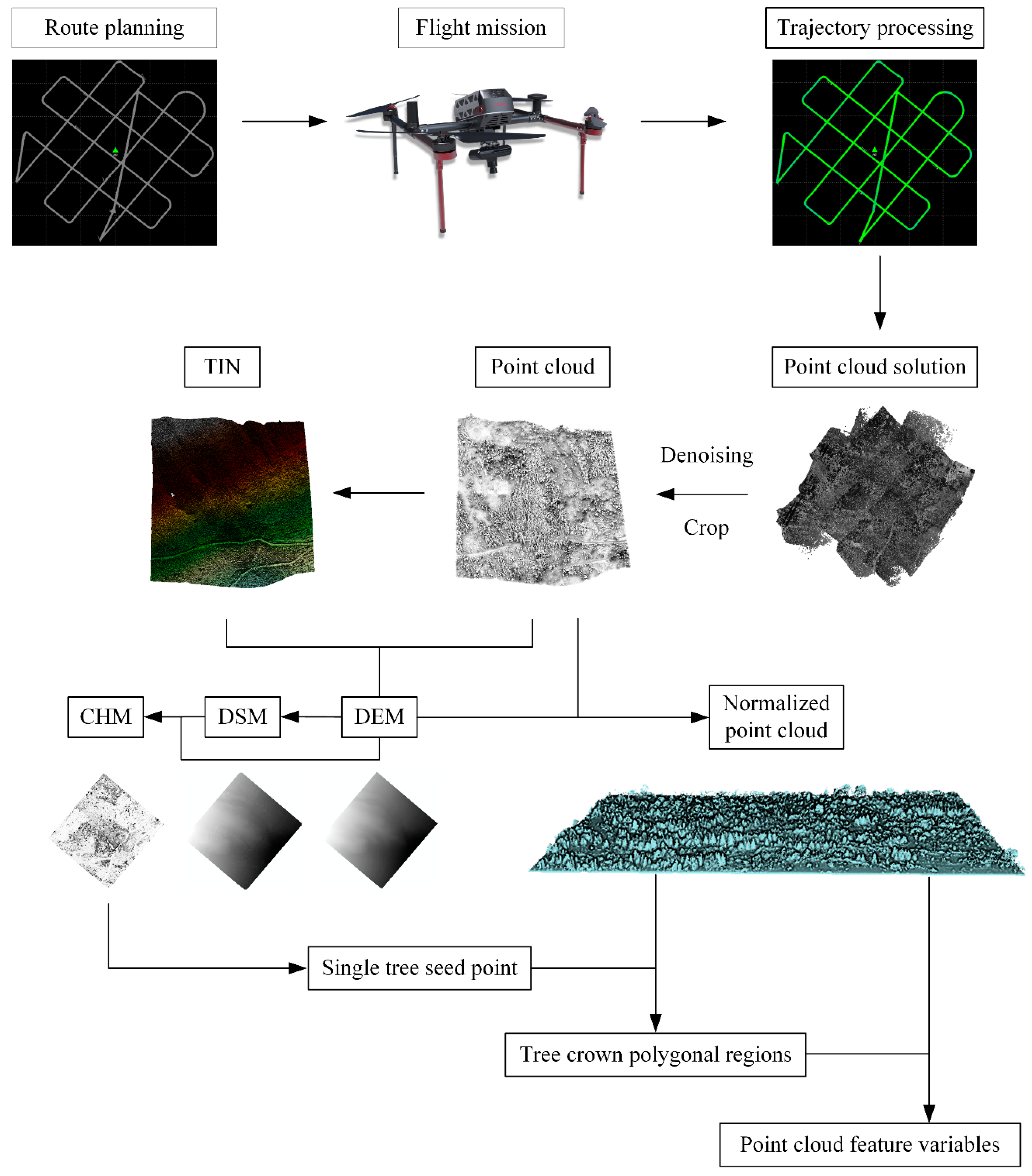
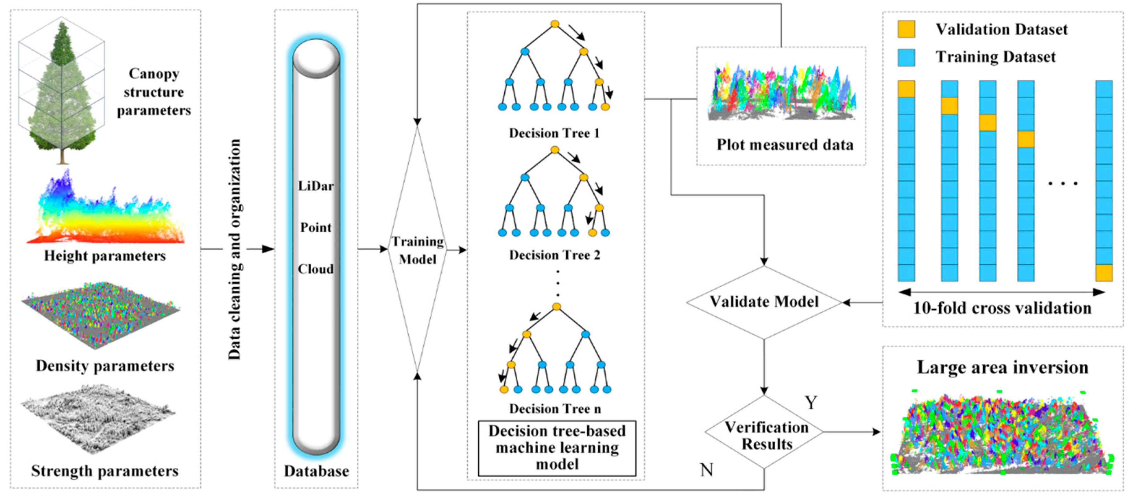
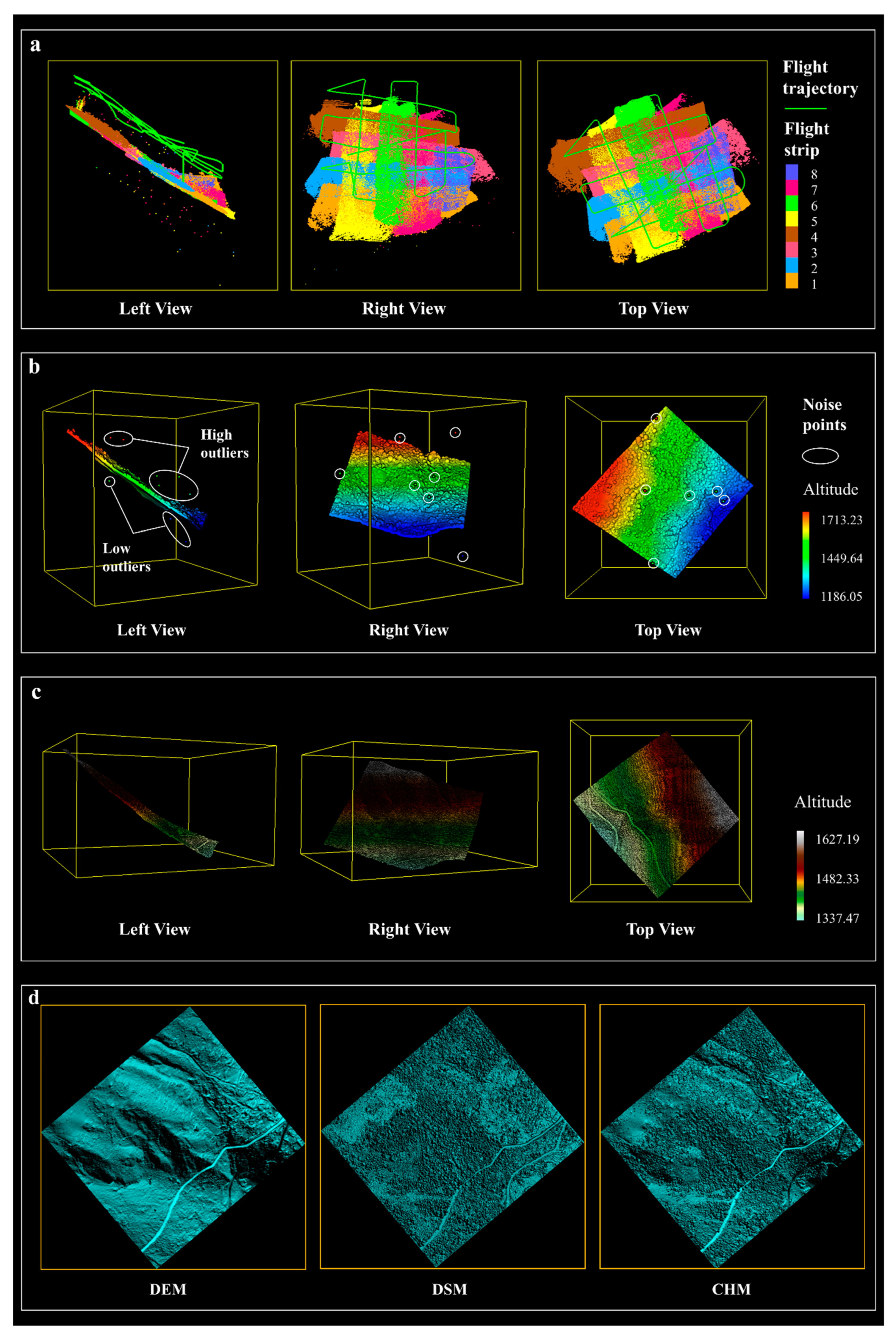
2.5. LiDAR Data Acquisition and Analysis

A high-precision airborne LiDAR survey was conducted in April 2024 using the Feima D2000 UAV system (Feima Robotics, Shenzhen, China) to enhance biomass estimation in the Luding region. Field investigations revealed that vegetation in the Luding region is unevenly distributed. To improve the accuracy of aboveground and belowground biomass estimation across the study area, airborne LiDAR was used to survey undisturbed regions. The LiDAR survey encompassed the undisturbed areas and extended beyond them, covering an area roughly ten times larger. The survey was conducted concurrently with field data collection under rain-free, low-wind, and low-tide conditions to minimize the influence of sampling time and weather on data quality. The Feima D2000 multirotor UAV system was equipped with a D-LiDAR2000 sensor (Feima Robotics, Shenzhen, China), an integrated Inertial Measurement Unit (IMU) (iPNS-2000), and a high-precision differential Global Navigation Satellite System (GNSS). The maximum takeoff weight was approximately 3.3 kg, supporting a flight duration of up to 70 min per mission. The UAV achieved a hovering accuracy of 1 cm + 1 ppm horizontally and 2 cm + 1 ppm vertically. The high-precision inertial navigation system provided a positioning accuracy of 0.02 m horizontally and 0.03 m vertically. The LiDAR module achieved centimeter-level ranging accuracy, operated at a pulse rate of 240 k pts/s, and supported a three-return echo function, enhancing penetration through vegetation for precise measurements.
A terrain-adaptive LiDAR survey was conducted, followed by trajectory processing and point cloud optimization for data acquisition (Figure 2). The survey area ranged in elevation from 1100 m to 1700 m, with a vertical drop exceeding 500 m. To ensure data accuracy, the flight path was designed for terrain-following operation at a relative altitude of 80 m, with a 50% flight path overlap, an average speed of 13 m/s, and an absolute field of view of 70°. After completing the flight mission, tightly coupled trajectory processing was performed using Novatel Inertial Explorer software (version 8.70), based on base station data, raw LiDAR data, and onboard IMU files. After validating the trajectory solution accuracy, point cloud preprocessing was conducted, including optimization adjustments and noise reduction. The final processed point cloud dataset, in LAS format, had an overall density of approximately 800 pts/m2.
Denoising, classification, and Triangulated Irregular Network (TIN)-based modeling were applied to process LiDAR data and extract vegetation metrics (Figure 2). For the acquired LAS point cloud data, a denoising algorithm with Nearest Neighbors set to 10 and a standard deviation multiplier of 5 was applied to remove high and low outliers. After denoising, an improved triangulated network filtering algorithm was used to classify ground points [30]. Due to the complex terrain structure and surface coverage in the study area, conventional ground point filtering was insufficient for accurate classification. Therefore, a high-density TIN was generated using the spike-free algorithm [31]. The TIN was then used to generate the 0.5 m resolution Digital Elevation Model (DEM) and Digital Surface Model (DSM). Then, the Canopy Height Model (CHM) was derived from the DSM and DEM, while the raw point cloud data were normalized. After extracting individual tree seed points from the CHM, tree crown polygonal regions were delineated based on the seed points and the normalized point cloud [32]. Subsequently, point cloud feature variables, including height metrics, intensity metrics, canopy closure, leaf area index (LAI), and gap fraction, were computed based on the polygons and normalized point cloud data.
To accurately extract individual tree characteristics from airborne point cloud data, decision tree-based machine learning algorithms were employed to model the relationship between point cloud data and individual trees (Figure 3). First, Spearman correlation analysis was used to select relevant point cloud feature variables. Then, several machine-learning algorithms, including Random Forest (RF), Gradient Boosting Machine (GBM), and Extreme Gradient Boosting (XGBoost), were compared in terms of model fitting performance and inversion error. GBM was ultimately selected as the optimal model. During model training, Bayesian Optimization was used for hyperparameter tuning, with 10-fold cross-validation applied to evaluate model performance. The optimization objectives were minimizing RMSE and maximizing R2, using field measurements from sample plots as training data. After model validation, the trained model was applied to large-scale forest stands for individual tree attribute inversion. Finally, aboveground and belowground biomass for the entire study area was estimated using an allometric growth equation.

3. Results

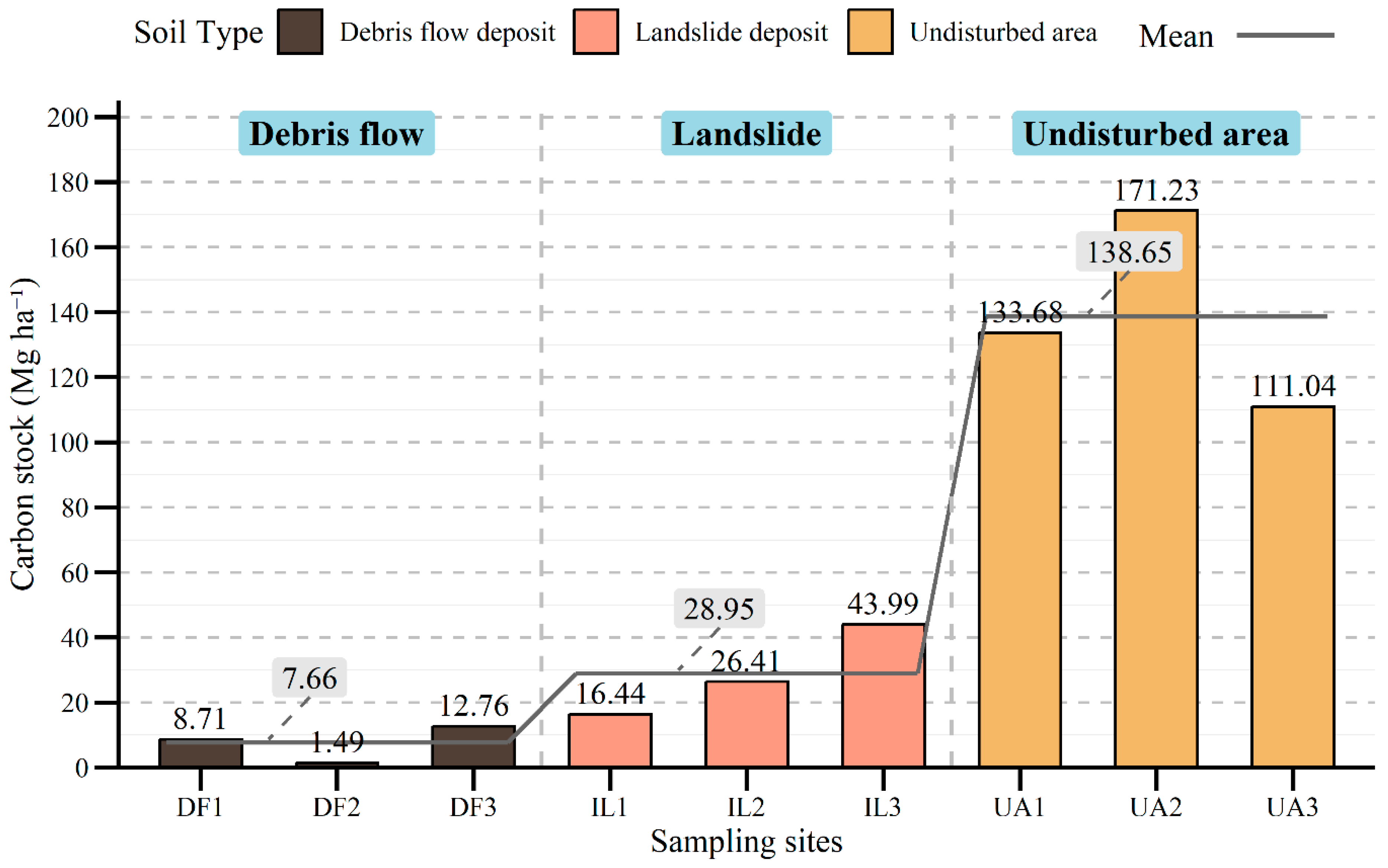
3.1. Soil Carbon Storage in Damaged Areas Dropped Significantly

Secondary disasters triggered by the Luding earthquake significantly reduced soil carbon storage in this region (Figure 4, Table S1). Within the 0–50 cm soil depth range, the highest soil carbon storage was observed in undisturbed areas (138.65 Mg/ha), followed by landslide deposits (28.95 Mg/ha), and the lowest in debris flow deposits (7.66 Mg/ha). The soil carbon storage in undisturbed areas was nearly five times that of landslide deposits. Compared to landslide deposits, soil carbon storage in debris flow deposits was further reduced to approximately one-fourth of that in landslide deposits. Overall, the undisturbed areas exhibited stable soil conditions with higher carbon storage, whereas landslide deposits, despite soil disturbance, retained a portion of their carbon storage. In debris flow deposits, only a minimal amount of organic carbon remained.
Descriptive statistics of soil organic carbon content and storage at different depths are presented in Table S1. From a vertical profile perspective, the undisturbed areas exhibited a gradual decline in soil organic carbon content and stock with increasing depth. The soil organic carbon stock in the 0–10 cm layer accounted for 27% of the total storage, approximately 1.8 times that in the 30–50 cm layer. In disturbed areas, soil carbon storage first increased and then decreased, with the 10–30 cm layer carbon storage lower than that in the subsoil, deviating from typical soil erosion patterns. Notably, the coefficients of variation for soil organic carbon fraction and soil carbon stock in the 0–10 cm layer of the debris flow zone reached 129.6% and 135.59%, respectively. Field investigations revealed that the high rock content in the study area’s soil is likely a key factor contributing to this anomaly, while long-term surface exposure may also be a contributing factor. One-way ANOVA of all sampling sites showed a significant effect of sampling location on soil carbon content and storage (p < 0.001), indicating that different sediment types significantly influenced soil carbon content. However, soil depth variation had no significant impact on soil carbon storage differences (p > 0.5).
Soil particle analysis provided further insights into soil development in the study area (Figure S3). Measurement data indicated that the average rock content in disturbed areas was approximately 83%, significantly higher than the 28% in undisturbed areas. Particle size analysis of sediments smaller than 10 mm revealed that over 81% were larger than 0.5 mm. Among different sediment types, undisturbed areas and debris flow deposits contained finer particles, whereas landslide deposits were dominated by coarse particles. Correlating the vertical distribution of soil organic carbon content with particle size revealed that smaller particles corresponded to higher soil organic carbon content.

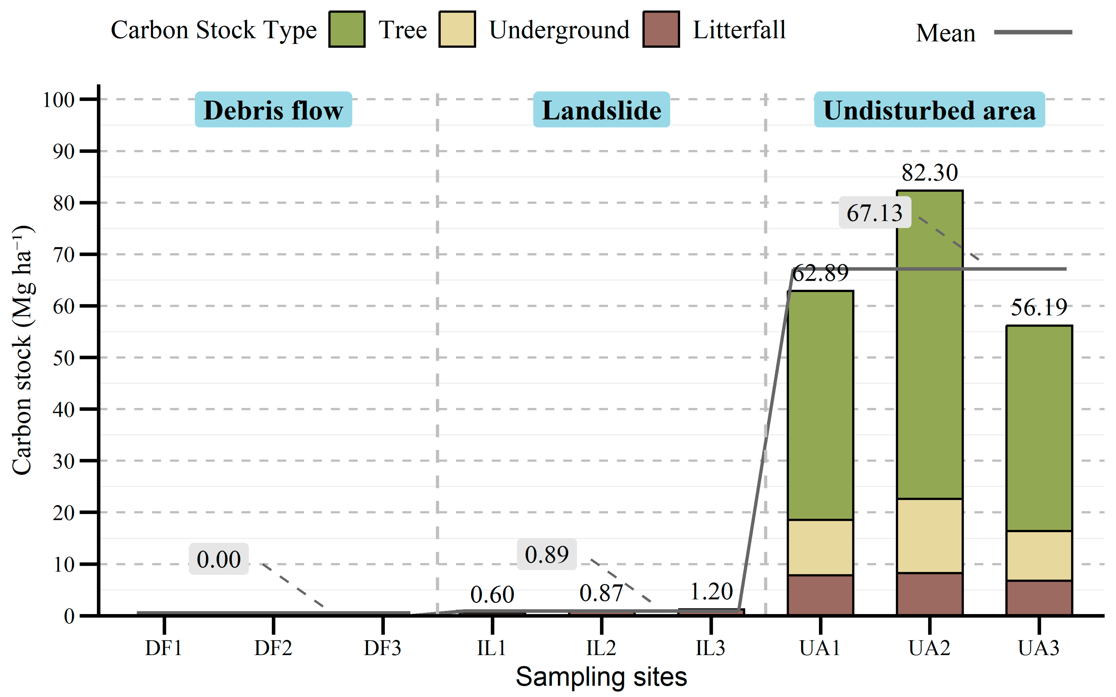
3.2. Secondary Disasters Stripped Away the Surface Vegetation

Measurement results indicate that vegetation carbon storage in the three undisturbed areas was 62.89 Mg/ha, 82.30 Mg/ha, and 56.19 Mg/ha, with an average value of 67.13 Mg/ha (Figure 5). Before the earthquake, vegetation carbon storage in undisturbed areas was primarily composed of aboveground biomass, accounting for approximately 71%. After the earthquake, vegetation in the disturbed areas was almost completely destroyed, and the ecosystem showed no clear signs of new vegetation recovery. Only a small amount of residual tree debris was found in landslide deposits, which was weighed on-site and treated as litterfall (Figure S1). Vegetation carbon storage in landslide and debris flow areas was significantly lower than in undisturbed regions. The landslide area retained only a minimal amount of carbon storage, primarily in the form of tree debris, while vegetation carbon storage in debris flow areas was completely lost. The ANOVA analysis revealed statistically significant differences in vegetation carbon storage composition among different types of deposits (p < 0.001). Earthquake-induced ecological destruction led to a complete loss of vegetation carbon storage, with its loss ratio exceeding that of soil carbon storage.

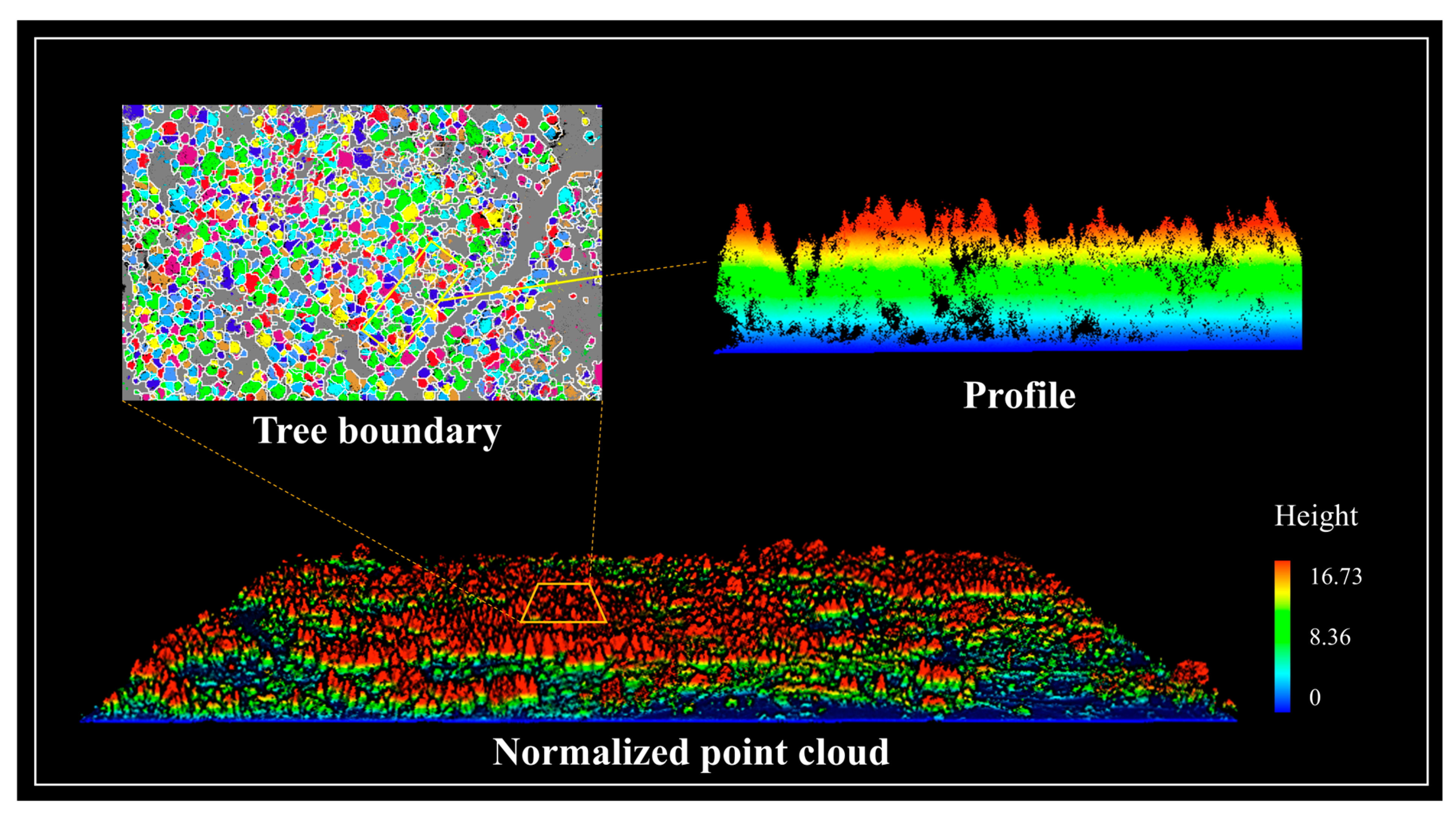
3.3. Inversion of Forest Biomass in Undisturbed Areas Based on LiDAR

The processed flight trajectory data for the study area are shown in Figure 6a, where darker green trajectory lines indicate higher processing accuracy. The actual data acquisition range exceeded the study area to ensure full coverage. However, lower point density at the edges, caused by large scanning angles, reduced data quality, necessitating the cropping of edge areas (Figure 6b). After cropping, the point cloud data still contained high and low outlier points. Denoising removed a total of 72,306 noise points, improving data quality. Ground point classification of the point cloud data produced a high-density TIN (Figure 6c). The TIN was rasterized to generate a DEM and DSM, from which a CHM was derived (Figure 6d).
Individual tree segmentation identified tree location, height, crown width, and boundaries of each tree. However, airborne LiDAR primarily captured the upper canopy, limiting its ability to characterize understory vegetation. Large-scale extraction of individual tree structural characteristics was achieved using the watershed algorithm on CHM, identifying tree crown polygons (Figure 7) [32]. In combination with normalized point cloud data, a total of 104 feature variables were extracted (Table S2). After statistical filtering, 53 variables significantly correlated with DBH (correlation coefficient > 0.3, p < 0.05) were selected for further analysis. The correlation matrix is shown in Figure S4. The study further compared the fitting performance of three decision tree-based algorithms—RF, GBM, and XGBoost. The model evaluation metrics (R2, RMSE, MAE) are presented in Table S3. The comprehensive evaluation results indicated that the model fitting performance ranked XGBoost > GBM > RF. Ultimately, GBM was selected as the final model, with validation results shown in Figure S5 (R2 = 0.823, RMSE = 1.18 cm).
Using the watershed algorithm, 4320 trees were identified in the LiDAR survey area, with tree heights ranging from 3.22 to 16.73 m, an average height of 6.72 m, and an average crown diameter of 3.46 m. After model fitting, the predicted DBH ranged from 4.54 to 13.22 cm, with an average of 7.02 cm. Among the model’s predictive variables, height had the highest relative importance, with the maximum tree height contributing approximately 28% (Figure S6). Using the allometric growth equation, the total aboveground biomass in the LiDAR survey area was estimated at approximately 66,767.94 kg, while belowground biomass was around 16,091.07 kg. Based on this estimation, the large-scale undisturbed areas in the study region had an aboveground carbon storage of approximately 33.38 Mg/ha and belowground carbon storage of 8.05 Mg/ha, which were lower than the average values measured at the three sample plots (47.96 Mg/ha and 11.56 Mg/ha, respectively).

3.4. Estimation of Carbon Loss in Ecosystems After the Earthquake

Debris flow deposits had the lowest ecosystem carbon storage, retaining only the soil carbon component. Landslide deposits had a slightly higher carbon storage, comprising soil carbon and a small amount of litterfall. The highest ecosystem carbon storage was observed in undisturbed areas, which included abundant soil carbon, biomass carbon, and litterfall. Specifically, in undisturbed areas, the average forest carbon storage was estimated based on LiDAR measurements (41.43 Mg/ha), while litterfall carbon storage was calculated using the average proportion from sample plots (5.29 Mg/ha). Combined with the soil carbon pool of 138.65 Mg/ha, the total ecosystem carbon storage was approximately 185.37 Mg/ha. Soil organic carbon was the primary component of the total ecosystem carbon pool, accounting for 74.8% in undisturbed conditions. In disturbed areas, the total ecosystem carbon storage was estimated at 29.84 Mg/ha in landslide deposits and 7.66 Mg/ha in debris flow deposits.

4. Discussion

Ecosystem carbon storage was reduced by 83.9% in landslides and by 95.9% in debris flow deposits, the latter exhibiting both the most severe carbon loss and the slowest vegetation recovery. This rapid carbon loss was primarily attributed to land cover changes, as landslides and debris flows stripped away surface vegetation and exposed the underlying soil. The resulting exposure intensified water erosion and physical disturbance, particularly in debris flow areas. These processes, along with increased soil porosity and structural disruption, further accelerated the decomposition and transfer of soil organic carbon [17,33]. The recovery of vegetation ecological functions in post-earthquake disturbed areas may take several years to decades. However, under typical conditions, some signs of recovery, such as the emergence of herbaceous plants, are expected in the second year after the earthquake [34,35]. However, this study found no significant signs of vegetation recovery in the Luding earthquake-affected areas within 1 year and 6 months post-earthquake, up to the sampling period.
Field sampling and UAV-based LiDAR improved carbon loss estimation, revealing that soil carbon accounted for 74.8% of total losses—far exceeding vegetation carbon loss. Most related studies currently rely on remote sensing imagery and vegetation indices (NDVI) to assess post-disaster ecosystem degradation [11,36,37]. However, these methods fail to accurately reflect the specific conditions of soil and forest carbon pools. Relying solely on satellite observations may underestimate the extent of damage caused by the earthquake disaster chain to local ecosystems. Based on field sampling and laboratory analysis, this study quantitatively estimated the carbon loss in post-earthquake ecosystems caused by land use change. Additionally, to further improve estimation accuracy, UAV-based LiDAR mapping was used to estimate forest biomass in undisturbed areas, correcting the previously overestimated biomass in sample plots by 30.4%. Notably, vegetation carbon storage accounted for only 25.2% of the total ecosystem carbon pool, while more severe losses occurred in the soil carbon pool—an insight that could not be obtained solely from remote sensing data.
Soil sieving and organic carbon analysis indicate that, in the absence of vegetation protection, a substantial amount of organic carbon is lost during erosion. High gravel content and limited soil development in the study area, combined with its complex topography, contribute to weak soil load-bearing capacity and high susceptibility to erosion. The rock content in disturbed areas is much higher than in undisturbed areas, and a large number of fine particles rich in organic carbon were transported away. The presence of coarser rock fragments in debris flow regions confirms their rheological properties, where coarse gravel remains in suspension during movement [38]. Studies have shown that approximately 10% of sediments are transported by debris flows [39], indicating that post-earthquake rainfall erosion is a primary driver of soil carbon migration in ecosystems. Our study also revealed a significant reduction in soil organic carbon content and a decline in soil cohesion in disturbed areas, further increasing the susceptibility to subsequent secondary disasters. Studies on other earthquake events have also confirmed that debris flow disasters remain frequent over extended periods following earthquakes [40].
Accurate acquisition of stand information is crucial for ecosystem service assessment, biomass estimation, and disaster loss evaluation, particularly in mountainous regions with complex terrain and uneven vegetation distribution like Luding [41,42]. Although sample plot surveys provide high accuracy, their large-scale application requires significant time, labor, and resources. Additionally, the situation in the Luding region highlights the advantages of UAV-based LiDAR mapping for forest biomass estimation [43]. This study utilized normalized UAV point cloud data and individual tree boundaries to extract point cloud feature variables and applied machine learning algorithms to estimate vegetation biomass in the study area. Unlike conventional CHM-based individual tree segmentation algorithms [44], this approach maximized point cloud information extraction and established a mapping relationship between airborne LiDAR and understory parameters. The study demonstrated that the decision tree-based GBM algorithm exhibited superior predictive performance and was more suitable for forest carbon storage estimation in this region. In this study, due to the unique terrain conditions, UAV-based biomass estimation demonstrated stronger representativeness than field measurements and offered greater cost-effectiveness.
Quantifying landslide-induced carbon loss is essential for understanding the ecological impact of the Luding earthquake. The total carbon loss in the region can be estimated by multiplying the measured average carbon loss per landslide (155.53 Mg/ha) by the total co-seismic landslide area [45]. We reviewed existing published landslide inventory studies and, through comparative analysis, determined that the inventory most recently developed by Zhao et al. is of higher quality and broader spatial coverage (47.3 km2), and thus was selected for this study [5,46,47]. The results indicate that the 47.3 km2 of landslides triggered by the Luding earthquake on 5 September 2022 resulted in an ecosystem carbon loss of approximately 7.36 × 10⁵ Mg. Previous research by Hilton et al. estimated that the large earthquake in the Western Southern Alps, New Zealand, resulted in a carbon transfer of 7.6 Mg C km−2 yr−1 over 40 years [6]. Jin et al. found that landslides in the Wenchuan earthquake region caused an ecosystem carbon loss of approximately 117.24 Mg/ha, accounting for 90% of the total loss, even after more than a decade of recovery [7]. These findings suggest that post-earthquake secondary disasters have led to significant carbon loss in local ecosystems.
This study quantified earthquake-induced carbon loss from a vertical ecosystem perspective, integrating field sampling and UAV observations to enhance estimation accuracy, although some limitations remain. First, this study used undisturbed areas as a reference for pre-earthquake conditions, which may introduce some uncertainty. Earthquakes can alter soil structure and forest photosynthesis, potentially affecting carbon storage in undisturbed areas. Also, representing the average carbon storage of landforms using data from sampling points may lead to over- or underestimation when extrapolating spatially. Second, this study did not account for carbon exchange within the lithosphere and focused solely on carbon transfer within the ecosystem. Finally, although UAV observations improved vegetation carbon storage estimation, the limited number of soil sampling sites may introduce uncertainty in soil organic carbon estimates.

5. Conclusions

This study assessed ecosystem carbon loss in the Luding earthquake-affected region using field sampling and UAV observations. The findings indicate that co-seismic landslides and debris flows significantly reduced vegetation and soil carbon storage, with losses ranging from 83.9% to 95.9%. Using publicly compiled landslide data, the study estimated that the Luding earthquake resulted in approximately 7.36 × 10⁵ Mg of carbon storage loss. UAV-derived point cloud data improved vegetation biomass estimation, reducing sample plot overestimation by 30.4%. This study is significant for understanding the carbon budget response of earthquake-affected ecosystems and contributes to a comprehensive understanding of the role of earthquakes in the carbon cycle. Furthermore, it provides a basis for post-disaster ecological restoration and reconstruction.

Supplementary Materials

The following supporting information can be downloaded at https://www.mdpi.com/article/10.3390/land14050915/s1, Table S1: Summary statistics of soil organic carbon content and soil organic carbon stock; Table S2: Point cloud feature variable statistics table; Table S3: Comparison of model performance metrics table; Figure S1: Field investigation photographs of the Luding earthquake; Figure S2: Schematic diagram of soil sampling plots. a, b, c are unaffected areas; d, e, f are debris flow sampling areas; g, h, i are landslide sampling areas; Figure S3: Soil particle size content in different deposits; Figure S4: Spearman correlation coefficient matrix of point cloud feature variables; Figure S5: Model validation results (a, jitter plot of predicted values and measured values; b, residuals plot); Figure S6: Top 20 variable importance based on information gain from the GBM.

Author Contributions

W.Z., writing—original draft, methodology, visualization, data curation, formal analysis; B.D., supervision, resources, funding acquisition, project administration, conceptualization; Y.Z., writing—review and editing, methodology; W.H., writing—review and editing, data collection; J.L., data collection, data curation; Z.Z., data collection, data curation; S.Y., data collection, data curation; T.M., visualization. All authors have read and agreed to the published version of the manuscript.

Funding

This study was supported by the National Key Research and Development Program of China (Grant No. 2023YFE0121900) and the National Natural Science Foundation of China (Grant No. 42377168).

Data Availability Statement

The raw data supporting the conclusions of this article will be made available by the authors on request.

Conflicts of Interest

The authors declare no conflicts of interest.

References

  1. Fan, X.; Scaringi, G.; Korup, O.; West, A.J.; van Westen, C.J.; Tanyas, H.; Hovius, N.; Hales, T.C.; Jibson, R.W.; Allstadt, K.E.; et al. Earthquake-Induced Chains of Geologic Hazards: Patterns, Mechanisms, and Impacts. Rev. Geophys. 2019, 57, 421–503. [Google Scholar] [CrossRef]
  2. Wu, X.; Xu, C.; Xu, X.; Chen, G.; Zhu, A.; Zhang, L.; Yu, G.; Du, K. A Web-GIS hazards information system of the 2008 Wenchuan Earthquake in China. Nat. Hazards Res. 2022, 2, 210–217. [Google Scholar] [CrossRef]
  3. Xu, C. Landslides triggered by the 2015 Gorkha, Nepal earthquake. Int. Arch. Photogramm. Remote Sens. Spatial Inf. Sci. 2018, XLII-3, 1989–1993. [Google Scholar] [CrossRef]
  4. Xu, C.; Xu, X.; Yao, X.; Dai, F. Three (nearly) complete inventories of landslides triggered by the May 12, 2008 Wenchuan Mw 7.9 earthquake of China and their spatial distribution statistical analysis. Landslides 2014, 11, 441–461. [Google Scholar] [CrossRef]
  5. Huang, Y.; Xie, C.; Li, T.; Xu, C.; He, X.; Shao, X.; Xu, X.; Zhan, T.; Chen, Z. An open-accessed inventory of landslides triggered by the MS 6.8 Luding earthquake, China on September 5, 2022. Earthq. Res. Adv. 2023, 3, 100181. [Google Scholar] [CrossRef]
  6. Hilton, R.G.; Meunier, P.; Hovius, N.; Bellingham, P.J.; Galy, A. Landslide impact on organic carbon cycling in a temperate montane forest. Earth Surf. Process. Landf. 2011, 36, 1670–1679. [Google Scholar] [CrossRef]
  7. Liu, J.; Fan, X.; Tang, X.; Xu, Q.; Harvey, E.L.; Hales, T.C.; Jin, Z. Ecosystem carbon stock loss after a mega earthquake. CATENA 2022, 216, 106393. [Google Scholar] [CrossRef]
  8. Cui, P.; Lin, Y.-M.; Chen, C. Destruction of vegetation due to geo-hazards and its environmental impacts in the Wenchuan earthquake areas. Ecol. Eng. 2012, 44, 61–69. [Google Scholar] [CrossRef]
  9. Cramer, W.; Bondeau, A.; Woodward, F.I.; Prentice, I.C.; Betts, R.A.; Brovkin, V.; Cox, P.M.; Fisher, V.; Foley, J.A.; Friend, A.D.; et al. Global response of terrestrial ecosystem structure and function to CO2 and climate change: Results from six dynamic global vegetation models. Glob. Change Biol. 2001, 7, 357–373. [Google Scholar] [CrossRef]
  10. Reichle, D.E. Bibliography, in the Global Carbon Cycle and Climate Change, 2nd ed.; Reichle, D.E., Ed.; Elsevier: Amsterdam, The Netherlands, 2023; pp. 571–652. [Google Scholar]
  11. Yunus, A.P.; Fan, X.; Tang, X.; Jie, D.; Xu, Q.; Huang, R. Decadal vegetation succession from MODIS reveals the spatio-temporal evolution of post-seismic landsliding after the 2008 Wenchuan earthquake. Remote Sens. Environ. 2020, 236, 111476. [Google Scholar] [CrossRef]
  12. Gomes, P.I.; Aththanayake, U.; Deng, W.; Li, A.; Zhao, W.; Jayathilaka, T. Ecological fragmentation two years after a major landslide: Correlations between vegetation indices and geo-environmental factors. Ecol. Eng. 2020, 153, 105914. [Google Scholar] [CrossRef]
  13. Wang, J.; Howarth, J.D.; McClymont, E.L.; Densmore, A.L.; Fitzsimons, S.J.; Croissant, T.; Gröcke, D.R.; West, M.D.; Harvey, E.L.; Frith, N.V.; et al. Long-term patterns of hillslope erosion by earthquake-induced landslides shape mountain landscapes. Sci. Adv. 2020, 6, eaaz6446. [Google Scholar] [CrossRef] [PubMed]
  14. Hilton, R.G.; West, A.J. Mountains, erosion and the carbon cycle. Nat. Rev. Earth Environ. 2020, 1, 284–299. [Google Scholar] [CrossRef]
  15. CENC. China Earthquake Networks Center. 2024. Available online: https://news.ceic.ac.cn/ (accessed on 10 March 2025).
  16. Fan, S.; Guan, F.; Xu, X.; Forrester, D.I.; Ma, W.; Tang, X. Ecosystem Carbon Stock Loss after Land Use Change in Subtropical Forests in China. Forests 2016, 7, 142. [Google Scholar] [CrossRef]
  17. Guan, F.; Tang, X.; Fan, S.; Zhao, J.; Peng, C. Changes in soil carbon and nitrogen stocks followed the conversion from secondary forest to Chinese fir and Moso bamboo plantations. CATENA 2015, 133, 455–460. [Google Scholar] [CrossRef]
  18. Coomes, D.A.; Allen, R.B.; A Scott, N.; Goulding, C.; Beets, P. Designing systems to monitor carbon stocks in forests and shrublands. For. Ecol. Manag. 2002, 164, 89–108. [Google Scholar] [CrossRef]
  19. Xiao, J.; Chevallier, F.; Gomez, C.; Guanter, L.; Hicke, J.A.; Huete, A.R.; Ichii, K.; Ni, W.; Pang, Y.; Rahman, A.F.; et al. Remote sensing of the terrestrial carbon cycle: A review of advances over 50 years. Remote Sens. Environ. 2019, 233, 111383. [Google Scholar] [CrossRef]
  20. Fan, G.; Zhang, B.; Zhou, J.; Wang, R.; Xu, Q.; Zeng, X.; Lu, F.; Luo, W.; Cai, H.; Wang, Y.; et al. Satellite Image Fusion Airborne LiDAR Point-Clouds-Driven Machine Learning Modeling to Predict the Carbon Stock of Typical Subtropical Plantation in China. Forests 2024, 15, 751. [Google Scholar] [CrossRef]
  21. Sun, H.Z.; Zhou, L.; Bao, F.; Wu, X. Landscape pattern and diversity of trees and shrubs in the alpine canyon area. J. Cent. South Univ. For. Technol. 2022, 42, 147–159. [Google Scholar] [CrossRef]
  22. Xu, X.; Cheng, J.; Xu, C.; Li, X.; Yu, G.; Chen, G.; Tan, X.; Wu, X. Discussion on block kinematic model and future themed areas for earthquake occurrence in the Tibetan Plateau: Inspiration from the Ludian and Jinggu earthquakes. Dizhen Dizhi 2014, 36, 1116–1134. [Google Scholar]
  23. Wang, L.; Li, Z.; Wang, D.; Liao, S.; Nie, X.; Liu, Y. Factors controlling soil organic carbon with depth at the basin scale. CATENA 2022, 217, 106478. [Google Scholar] [CrossRef]
  24. Odebiri, O.; Mutanga, O.; Odindi, J.; Slotow, R.; Mafongoya, P.; Lottering, R.; Naicker, R.; Matongera, T.N.; Mngadi, M. Remote sensing of depth-induced variations in soil organic carbon stocks distribution within different vegetated landscapes. CATENA 2024, 243, 108216. [Google Scholar] [CrossRef] [PubMed]
  25. Zhang, L.; Xie, Z.; Zhao, R.; Wang, Y. The impact of land use change on soil organic carbon and labile organic carbon stocks in the Longzhong region of Loess Plateau. J. Arid. Land 2012, 4, 241–250. [Google Scholar] [CrossRef]
  26. Pu, W.; Zhao, M.; Du, J.; Liu, Y.; Huang, C. Effect of Geographical Conditions on Moss–Soil Crust Restoration on Cut Rock Slopes in a Mountainous Area in Western Sichuan, China. Sustainability 2023, 15, 1990. [Google Scholar] [CrossRef]
  27. Xie, Z.; Zhu, J.; Liu, G.; Cadisch, G.; Hasegawa, T.; Chen, C.; Sun, H.; Tang, H.; Zeng, Q. Soil organic carbon stocks in China and changes from 1980s to 2000s. Glob. Change Biol. 2007, 13, 1989–2007. [Google Scholar] [CrossRef]
  28. Zeng, W. Assessment of Individual Tree Above- and Below-Ground Biomass Models for 34 Tree Species in China; Book Publisher International: Bhanjipur, India, 2020; pp. 26–37. [Google Scholar]
  29. IPCC. Climate Change 2022: Impacts, Adaptation, and Vulnerability. Contribution of Working Group II to the Sixth Assessment Report of the Intergovernmental Panel on Climate Change; Pörtner, D.C.R.H.-O., Tignor, M., Poloczanska, E.S., Mintenbeck, K., Alegría, A., Craig, M., Langsdorf, S., Löschke, S., Möller, V., Okem, A., et al., Eds.; Cambridge University Press: Cambridge, UK; New York, NY, USA, 2022; 3056p. [Google Scholar]
  30. Zhao, X.; Guo, Q.; Su, Y.; Xue, B. Improved progressive TIN densification filtering algorithm for airborne LiDAR data in forested areas. ISPRS J. Photogramm. Remote Sens. 2016, 117, 79–91. [Google Scholar] [CrossRef]
  31. Khosravipour, A.; Skidmore, A.K.; Isenburg, M. Generating spike-free digital surface models using LiDAR raw point clouds: A new approach for forestry applications. Int. J. Appl. Earth Obs. Geoinf. 2016, 52, 104–114. [Google Scholar] [CrossRef]
  32. Chen, Q.; Baldocchi, D.; Gong, P.; Kelly, M. Isolating Individual Trees in a Savanna Woodland using Small Footprint LIDAR data. Photogramm. Eng. Remote Sens. 2006, 72, 923–932. [Google Scholar] [CrossRef]
  33. Wang, Q.; Wang, S.; Yu, X. Decline of soil fertility during forest conversion of secondary forest to Chinese fir plantations in subtropical China. Land Degrad. Dev. 2011, 22, 444–452. [Google Scholar] [CrossRef]
  34. Wang, X.; Fan, X.; Fang, C.; Dai, L.; Zhang, W.; Zheng, H.; Xu, Q. Long-Term Landslide Evolution and Restoration After the Wenchuan Earthquake Revealed by Time-Series Remote Sensing Images. Geophys. Res. Lett. 2024, 51, e2023GL106422. [Google Scholar] [CrossRef]
  35. Schomakers, J.; Jien, S.-H.; Lee, T.-Y.; Huang, J.-C.; Hseu, Z.-Y.; Lin, Z.L.; Lee, L.-C.; Hein, T.; Mentler, A.; Zehetner, F. Soil and biomass carbon re-accumulation after landslide disturbances. Geomorphology 2017, 288, 164–174. [Google Scholar] [CrossRef] [PubMed]
  36. Wang, J.; Wang, Z.; Cheng, H.; Kang, J.; Liu, X. Land Cover Changing Pattern in Pre- and Post-Earthquake Affected Area from Remote Sensing Data: A Case of Lushan County, Sichuan Province. Land 2022, 11, 1205. [Google Scholar] [CrossRef]
  37. Mi, H.; Cui, J.; Ning, Y.; Liu, Y.; Zhu, M. Post-earthquake recovery monitoring and driving factors analysis of the 2014 Ludian Ms6.5 earthquake in Yunnan, China based on LUCC. Stoch. Environ. Res. Risk Assess. 2023, 37, 4991–5007. [Google Scholar] [CrossRef]
  38. Pierson, T.C. Dominant particle support mechanisms in debris flows at Mt Thomas, New Zealand, and implications for flow mobility. Sedimentology 1981, 28, 49–60. [Google Scholar] [CrossRef]
  39. Francis, O.; Fan, X.; Hales, T.; Hobley, D.; Xu, Q.; Huang, R. The Fate of Sediment After a Large Earthquake. J. Geophys. Res. Earth Surf. 2022, 127, e2021JF006352. [Google Scholar] [CrossRef]
  40. Yang, W.; Qi, W.; Zhou, J. Decreased post-seismic landslides linked to vegetation recovery after the 2008 Wenchuan earthquake. Ecol. Indic. 2018, 89, 438–444. [Google Scholar] [CrossRef]
  41. McKinley, D.C.; Ryan, M.G.; Birdsey, R.A.; Giardina, C.P.; Harmon, M.E.; Heath, L.S.; Houghton, R.A.; Jackson, R.B.; Morrison, J.F.; Murray, B.C.; et al. A synthesis of current knowledge on forests and carbon storage in the United States. Ecol. Appl. 2011, 21, 1902–1924. [Google Scholar] [CrossRef]
  42. Nakata, Y.; Hayamizu, M.; Ishiyama, N. Assessing primary vegetation recovery from earthquake-induced landslide scars: A real-time kinematic unmanned aerial vehicle approach. Ecol. Eng. 2023, 193, 107019. [Google Scholar] [CrossRef]
  43. Navarro, A.; Young, M.; Allan, B.; Carnell, P.; Macreadie, P.; Ierodiaconou, D. The application of Unmanned Aerial Vehicles (UAVs) to estimate above-ground biomass of mangrove ecosystems. Remote Sens. Environ. 2020, 242, 111747. [Google Scholar] [CrossRef]
  44. Song, Z.; Tomasetto, F.; Niu, X.; Yan, W.Q.; Jiang, J.; Li, Y. Enabling Breeding Selection for Biomass in Slash Pine Using UAV-Based Imaging. Plant Phenomics 2022, 2022, 9783785. [Google Scholar] [CrossRef]
  45. Dai, W.; Fu, W.; Jiang, P.; Zhao, K.; Li, Y.; Tao, J. Spatial pattern of carbon stocks in forest ecosystems of a typical subtropical region of southeastern China. For. Ecol. Manag. 2018, 409, 288–297. [Google Scholar] [CrossRef]
  46. Zhang, J.-Q.; Yang, Z.-J.; Meng, Q.-K.; Wang, J.; Hu, K.-H.; Ge, Y.-G.; Su, F.-H.; Zhao, B.; Zhang, B.; Jiang, N.; et al. Distribution patterns of landslides triggered by the 2022 Ms 6.8 Luding earthquake, Sichuan, China. J. Mt. Sci. 2023, 20, 607–623. [Google Scholar] [CrossRef]
  47. Zhao, B.; Su, L.; Qiu, C.; Lu, H.; Zhang, B.; Zhang, J.; Geng, X.; Chen, H.; Wang, Y. Understanding of Landslides Induced by 2022 Luding Earthquake, China. J. Rock Mech. Geotech. Eng. 2024, in press. [CrossRef]
Figure 1. Geographic location of the study area. The red polygons represent the spatial distribution of co-seismic landslides after the earthquake, derived from publicly available compiled landslide data. DF1~3 indicate debris flow deposit sampling sites; IL1~3 indicate inactive landslide deposit sampling sites; UA1~3 indicate sampling sites in unaffected areas.
Land 14 00915 g001
Figure 2. Flowchart of point cloud data acquisition and forest parameter acquisition.
Land 14 00915 g002
Figure 3. Flowchart of inverting single tree characteristics based on machine learning algorithm.
Land 14 00915 g003
Figure 4. Soil organic carbon stock in original and damaged areas.
Land 14 00915 g004
Figure 5. Vegetation carbon stock in original and damaged areas.
Land 14 00915 g005
Figure 6. LiDAR data processing and CHM generation. (a) Processed flight trajectory; (b) Edge cropping; (c) TIN from ground point classification; (d) Rasterized DEM and DSM, and derived CHM.
Land 14 00915 g006
Figure 7. Single tree boundary based on CHM and normalized point cloud.
Land 14 00915 g007
Disclaimer/Publisher’s Note: The statements, opinions and data contained in all publications are solely those of the individual author(s) and contributor(s) and not of MDPI and/or the editor(s). MDPI and/or the editor(s) disclaim responsibility for any injury to people or property resulting from any ideas, methods, instructions or products referred to in the content.

