Article

Spatiotemporal Land Use and Land Cover Changes and Their Impact on Landscape Patterns in the Colombian Coffee Cultural Landscape (2014–2034)

by
Anyela Piedad Rojas Celis
1,
Jie Shen
1,2,* and
Jose David Martinez Otalora
1
1
College of Civil Engineering and Architecture, Zhejiang University, Hangzhou 310058, China
2
Center for Balance Architecture, Zhejiang University, Hangzhou 310058, China
*
Author to whom correspondence should be addressed.
Land 2025, 14(5), 1045; https://doi.org/10.3390/land14051045
Submission received: 18 March 2025 / Revised: 5 May 2025 / Accepted: 7 May 2025 / Published: 11 May 2025

Abstract

:
The Colombian Coffee Cultural Landscape (CCLC), a UNESCO World Heritage site, faces conservation threats due to changes in land use and land cover (LULC). This study analyzed and predicted the spatiotemporal dynamics of LULC in the CCLC from 2014 to 2034, assessing its effects on the landscape structure. The analyses identified negative impacts and provided insights for developing conservation and land use planning strategies aimed at comprehensive landscape management. A supervised classification methodology using the Random Forest algorithm was implemented by integrating multispectral (Landsat 8) and Synthetic Aperture Radar (SAR) data (Sentinel-1), achieving an overall accuracy of 87.88% and a Kappa coefficient of 84.20%. Future projections were conducted using a hybrid Cellular Automata and Artificial Neural Network model (CA-ANN), reaching an accuracy of 88.12% and a Kappa coefficient of 0.84. The results indicate urban expansion, increasing from 1.46% in 2014 to 15.64% by 2034, accompanied by a forest cover loss of 77.8% and a reduction in coffee-growing areas from 77.91% in 2019 to 68.40% by 2034. Landscape metric analysis revealed increased fragmentation and spatial heterogeneity. The integration of multisensor remote sensing, hybrid predictive models, and landscape metrics within the CCLC provides a quantitative methodological framework to evaluate the transformation of cultural landscapes under anthropogenic pressures.

Graphical Abstract

1. Introduction

Cultural landscapes, recognized for their Outstanding Universal Value (OUV) by the United Nations Educational, Scientific and Cultural Organization UNESCO [1], are experiencing accelerated transformations due to changes in land use and land cover (LULC) [2]. Globally, it is estimated that nearly three quarters of the Earth’s surface have been transformed by human activities [3,4], exacerbating habitat fragmentation, biodiversity loss, and the degradation of cultural values [5]. This phenomenon not only affects natural ecosystems but also areas designated as World Heritage Sites, such as Sagarmatha National Park in Nepal [6], Jeju Island in the Republic of Korea [7], and the Viñales Valley in Cuba [8], where urbanization, deforestation, and agricultural expansion processes have been documented, compromising their integrity. Similar pressures, notably from urbanization and agricultural expansion, also threaten the integrity of the Colombian Coffee Cultural Landscape (CCLC). These changes reflect the direct interaction between human activities and the natural environment, driven by socioeconomic and environmental factors [9]. Over time, human intervention has shaped productive landscapes with high economic, cultural, and ecological value; however, growing anthropogenic pressure jeopardizes their sustainability [10].
LULC change directly affects landscape patterns, defined as the spatial organization of territorial elements according to their distribution, size, shape, and characteristics [11,12]. These configurations are manifestations of LULC changes [13,14] that do not occur in isolation but are the result of a complex interaction between natural processes and socioeconomic dynamics [15,16]. In the case of heritage cultural landscapes, these transformations can alter both the physical structure of the territory and the cultural values and traditional practices that have historically characterized them. Therefore, understanding the relationship between LULC dynamics and landscape patterns is fundamental for their sustainable management and preservation.
Various studies have addressed aspects related to the processes and trends in land use change [17,18], the identification of mechanisms derived from human activities [19], and the response of land use to landscape patterns [20]. Furthermore, methodological approaches have been developed, such as the multisensor integration of optical data from Landsat 8 and SAR data from Sentinel-1 for LULC analysis, the application of hybrid models based on CA-ANN for future predictions, and the analysis of landscape metrics using the FRAGSTATS 4.3 software, which have been widely documented in the scientific literature [21,22,23]. However, there is a lack of studies that assess the current state and project the gradients of change and trajectories of transformation of the Colombian Coffee Cultural Landscape CCLC [24], which hampers the design of effective strategies for its sustainable management.
The Colombian Coffee Cultural Landscape was declared a World Heritage Site by UNESCO in 2011 under criteria (v) and (vi) [25]. This recognition distinguishes it as an exceptional example of a traditional human settlement and sustainable land management, where the interaction between local cultures and the environment converges with the preservation of living traditions and intangible cultural elements of universal value. The CCLC is characterized by a unique agricultural landscape and shaped by traditional practices that have contributed to food security, economic development, and the preservation of its distinctive scenic value [26]. However, it faces increasing threats such as changes in land use, natural disasters, climate change, urban expansion, and rising tourism [27,28,29]. These pressures have generated significant alterations, including habitat fragmentation, risks to food security, and the loss of ancestral knowledge, thereby endangering the sustainability of the cultural heritage.
In the context of the rapid transformation of land use and land cover in the CCLC, it is essential to understand the spatiotemporal dynamics of LULC and its impact on landscape patterns. Therefore, the objectives of this study are as follows:
  • To classify and validate the accuracy of land use and land cover categories for the period 2014–2024;
  • To predict LULC transformations for 2034;
  • To quantitatively compare and characterize the spatial and temporal evolution of changes in LULC and their effects on landscape patterns;
  • To understand the relationship between LULC dynamics and changes in landscape patterns by analyzing the gradients of change and trajectories of transformation.

2. Materials and Methods

2.1. Study Area

The Colombian Coffee Cultural Landscape (CCLC) is located on the central and western slopes of the Andes mountain range, within the mid-elevation mountainous regions ranging from 1000 to 1900 m above sea level. The area is characterized by temperatures between 17 and 24 °C and annual precipitation ranging from 1200 to 2300 mm. It extends across the departments of Caldas, Quindío, Risaralda, and Valle del Cauca, with a total population of 595,884 inhabitants. The territory is composed of six distinct landscape zones—Zone A through Zone F, as shown in Figure 1b, which are characterized by the integration of cultural traditions, including the expressions of Indigenous and Afro-descendant communities, archeological heritage, historical town centers, and legacies associated with coffee cultivation. The region also displays a diverse pattern of land use and agricultural production, encompassing extensive coffee plantations, agroforestry systems, grazing areas, patches of native vegetation, and urban centers with commercial and tourism-related activities [26].
The CCLC is divided into two zones. The primary zone corresponds to the core area, which spans 141,120 hectares—of which 140,046 hectares are rural and 1074 hectares are urban—distributed across 47 municipalities, 411 rural settlements (veredas), and 14 urban centers. The buffer zone covers 207,000 hectares, comprising 204,542 hectares of rural land and 2458 hectares of urban land, distributed across 51 municipalities, 447 veredas, and 17 urban centers.
This study focuses exclusively on the core zone of the Colombian Coffee Cultural Landscape (CCLC), where the attributes that justify its inscription under the Outstanding Universal Value (OUV) criteria are officially located [30]. According to UNESCO guidelines, only the core zone is considered part of the designated World Heritage property, while the buffer zone serves a complementary role in protection and management [31,32]. From a conservation standpoint, land use changes within the core area have a direct impact on the authenticity and integrity of the landscape. Methodologically, the core zone provides a clearly defined and spatially coherent unit for analysis, enabling the more accurate application of spatial metrics and predictive modeling. Including the buffer zone, which exhibits greater heterogeneity and lacks formal recognition as part of the inscribed site, could introduce analytical inconsistencies and dilute the interpretation of landscape dynamics related to the OUV [2].

2.2. Dataset

To generate the LULC maps, a multisensor database was compiled for the 2014–2024 period using image collections from the Google Earth Engine (GEE, Google LLC, Mountain View, CA, USA; web service version accessed 8 August 2024), managed by the United States Geological Survey (USGS). Data processing was performed entirely on the GEE platform using cloud-based computing. As summarized in Table 1, additional predictor variables were incorporated to forecast LULC changes from 2024 to 2034, including the following: elevation, slope, aspect, population, distance to roads, and distance to rivers. Population data were obtained from the WorldPop Global Project, road networks from OpenStreetMap, and river networks from the New Global Hydrography dataset. Elevation and slope were derived from the 30 m resolution Digital Elevation Model of the Shuttle Radar Topography Mission (SRTM). Temperature data were extracted from the ERA5-Land Daily Aggregated product, precipitation data from the CHIRPS Daily dataset, and Normalized Difference Vegetation Index (NDVI) values from the Landsat 8 NDVI 8-Day Composite. All environmental variables were sourced directly from GEE, ensuring consistency in spatial resolution (30 m) and temporal coverage across the study period.

2.3. Methodology

This study was structured into three main components: (1) LULC classification, (2) projection of future LULC under a Business as Usual (BAU) scenario, and (3) the spatiotemporal analysis of LULC changes and landscape patterns, as shown in Figure 2. The first section encompassed the processing, classification, and validation of LULC. In this section, a multisensor supervised classification methodology for LULC analysis was implemented [33,34,35], integrating optical data from Landsat 8 and radar data from Sentinel-1 during the period 2014–2024. The integration of optical and SAR data combined the spectral information of the surface with structural and roughness data, thereby overcoming the limitations of each sensor.
For the second section, spatiotemporal transitions and the future scenarios of LULC for 2034 were modeled using the Modules for Land-Use Change Evaluation (MOLUSCE) plugin in QGIS 3.4 Bratislava (QGIS.ORG Association, Bern, Switzerland), which is employed to simulate changes in land use and land cover.
In the final section, the moving window method in FRAGSTATS v 4.2 (University of Massachusetts Amherst, Amherst, MA, USA) was applied to analyze the spatiotemporal variations in LULC and landscape patterns. The integration of spatial representation approaches facilitated the development of an extensive set of metrics that characterized the structure and spatial configuration in greater detail, thereby contributing to a better understanding of landscape dynamics.

2.3.1. LULC Classification

Satellite Image Processing

The processing of Landsat 8 Collection 2 Tier 1 Level 2 imagery included atmospheric correction using the LaSRC algorithm [36], with cloud and shadow masks generated from the QA_PIXEL band [37], all processed in Google Earth Engine (GEE) [38,39,40]. For temporal integration, a median filter was applied to produce a composite image [41,42]. Additionally, Sentinel-1 SAR imagery (IW mode, VV/VH polarizations) was processed by applying speckle filtering and computing the VV/VH ratio [43,44]. All layers were standardized to the EPSG:4326 coordinate reference system and resampled to a spatial resolution of 30 m.

Application of Spectral Indices

The spectral characterization of land cover in the CCLC was based on validated indices for discriminating coffee crops, forests, bamboo, grasslands, water bodies, bareland, and built-up areas [22,45,46]. Using the bands from the Landsat 8 OLI sensor (blue, green, red, and near-infrared) [47,48], ten indices were computed: the Enhanced Vegetation Index (EVI) to differentiate canopy structures [49,50,51,52]; the Normalized Difference Vegetation Index (NDVI), the Soil-Adjusted Vegetation Index (SAVI), and the Modified Soil-Adjusted Vegetation Index (MSAVI) to distinguish young coffee crops from grasslands [53,54,55,56,57,58]; the Normalized Difference Built-up Index (NDBI) and the Urban Index (UI) for built-up areas [59,60,61,62,63]; the Bare Soil Index (BSI) for exposed soils [64,65]; and the Modified Normalized Difference Water Index (MNDWI), the Normalized Difference Moisture Index (NDMI), and the Land Surface Water Index (LSWI) for water bodies and soil moisture [66,67,68,69,70,71]. These indices were integrated as additional bands into the annual composites, thereby optimizing the discrimination among LULC classes. The spectral indices, formulas, and references used in the classification are listed in Table S1.

Supervised Classification

Supervised classification is a method that employs labeled training samples to guide the categorization of pixels into different land use and land cover (LULC) classes [72]. For this study, a representative set of samples covering the relevant LULC categories in the analysis area was selected. These samples were used to train a classification model based on Random Forest (RF), assigning each pixel to one of the defined classes [73,74]. RF is a multivariate and non-parametric machine learning algorithm that improves classification accuracy by combining multiple decision trees [75]. In this study, RF was employed for the multitemporal classification of LULC into seven specific classes.

Definition of Classes

Seven land use and cover (LULC) classes were identified: built-up land, coffee crops, bareland, forest, grasslands, bamboo, and water bodies. Supervised classification algorithms employed labeled samples to recognize the spectral patterns associated with each class [76]. The trained model was applied to both historical and current images, enabling the detection of changes such as urban expansion or the conversion of forests to agricultural land [77]. Training and validation samples were generated through the visual interpretation of Landsat 8 and Sentinel-1 composite images available on GEE. A detailed description of each class, including its uses and characteristics, is presented in Table 2.

LULC Validation Process

The validation method employed in this study involved the random partitioning of data into training and validation sets. A total of 80% of the samples were allocated for training the Random Forest classifier, while the remaining 20% were proportionally distributed among the categories for validation [78,79]. This data-splitting approach is widely recommended to ensure a robust evaluation of the model [80].
Confusion matrices were generated for each period analyzed, enabling the calculation of statistical metrics, including overall accuracy (OA), user accuracy (UA), producer accuracy (PA), and the Kappa coefficient [81]. Additionally, to gain deeper insights into specific types of classification errors, the Quantity Disagreement (QD) and Allocation Disagreement (AD) metrics were calculated, as proposed by Pontius and Millones [82]. Quantity Disagreement quantifies errors due to differences in classified versus observed class areas, while Allocation Disagreement measures errors related to the spatial misallocation of classes. These metrics are essential for evaluating the performance of LULC classification models, providing a quantitative measure of their accuracy [83,84]. The described procedure was implemented in a script on Google Earth Engine (GEE), the details of which are presented in Appendix A.

2.3.2. Method for LULC in 2034 Prediction

Spatial Variables

The spatial variables used for prediction included natural factors: elevation, slope [85], precipitation, temperature, and NDVI vegetation dynamics [86,87]; neighborhood factors: distance to main roads and proximity to bodies of water [88]; and socioeconomic aspects, such as population density [89]. The raster maps of each variable (Figure 3) were standardized to a resolution of 30 m, with NoData values set to 0, and a unified spatial extent and coordinate system (ESRI:31918—SIRGAS_UTM_Zone_18N) were applied, thereby ensuring consistency across all spatial layers used. These variables are employed in land use/land cover (LULC) change analysis [90,91,92], as they provide reproducible information regarding the physical and anthropogenic influences on its evolution. The 30 m WorldPop population dataset was chosen to match the resolution of the Landsat and Sentinel imagery, facilitating the integration of demographic and environmental layers in the modeling process.

Prediction and Validation of Models with MOLUSCE

The MOLUSCE plugin is widely used in modeling land use changes [90]. It provides robust methods for evaluating the correlation between LULC data and spatial variables. Natural, socioeconomic, and neighborhood factors have been identified as key drivers of land use change [93]. LULC simulation was performed using the CA-ANN algorithm, which was implemented in the MOLUSCE module of QGIS [90]. This approach combined Cellular Automata (CA) which model the spatial dynamics with Artificial Neural Networks (ANN) that capture the non-linear relationships between explanatory variables and land use change.
The modeling was conducted under a Business as Usual (BAU) scenario. This scenario assumed that the land use transition probabilities and spatial driving forces observed during the calibration period (2019–2024) would persist into the projection period (2024–2034). Consequently, the model extrapolated existing trends, including accelerated transformations if such dynamics were detected in the recent past.
The process was carried out in two stages. First, the model was trained and validated to predict the LULC for 2024 using historical data from 2014 and 2019, by integrating explanatory variables and transition matrices. Validation was performed using the Kappa index, achieving an overall accuracy of 86.52% and a Kappa index of 0.83. Subsequently, the validated model was used to project the LULC for 2034, incorporating the LULC data of 2019 and 2024, along with the same explanatory variables and transition matrices employed in the validation stage. The CA-ANN model was configured with 350 iterations, a neighborhood size of 1 × 1 pixels, a learning rate of 0.005, five hidden layers, and a momentum of 0.010.

2.3.3. Spatiotemporal Analysis Methods

Transition Matrices and Chord Diagrams

To analyze LULC changes, transition matrices were employed as a fundamental tool [94]. In the matrix, the rows and columns corresponded to the land use types in two distinct periods (T1 and T2). The values within the matrix (Mij, where i, j = 1, 2, …, n) represented the areas that had experienced changes among the different land use types during both periods. This method was based on previous studies [95,96].

Moving Window Method

The moving window method was implemented to generate a grid map of landscape indices, allowing for the evaluation of the spatial variability of landscape patterns at different scales [97,98]. A 100 m × 100 m window was used, systematically shifted from the upper-left corner of the study area. At each position, landscape indices were calculated and assigned to the central cell.
The window size was determined after evaluating multiple scales, with the objective of minimizing distortion in the results and maximizing the representativeness of spatial patterns. For each window position, landscape indices were calculated using FRAGSTATS 4.3 software [99], considering data from four temporal periods (2014, 2019, 2024, and 2034).

Land Use Degree Index (LUDI)

The Land Use Degree Index (LUDI) is a quantitative indicator that measures the magnitude and depth of transformations in land use/land cover (LULC). This index facilitates the analysis of the interaction between natural systems and anthropogenic activities in landscape configuration, providing a comprehensive perspective on land occupation [100].
The degree of land use is defined at multiple levels based on the equilibrium state of natural ecosystems under socioeconomic influences, thereby establishing a classification index (Table 3). For its calculation, an intensity value is assigned to each land use category to reflect the degree of anthropogenic alteration. The LUDI is computed as the weighted sum of the percentage of the area occupied by each category and its respective intensity index, as expressed in the following equation:
L d = 100 × i n = 1   ( B i × C i ) ; L d a [ 100 , 400 ]
where
  • Ld represents the comprehensive land use intensity index for the study area.
  • Bi corresponds to the intensity index assigned to the category.
  • Ci indicates the percentage of the surface occupied by the category.
  • i denotes the land use category number.
  • n is the total number of evaluated categories.

Spatial Autocorrelation Analysis

To analyze the characteristics of spatial autocorrelation in land use intensity, this study implemented two complementary techniques: global Moran’s I index and the Local Indicators of Spatial Association (LISA) [101,102]. The LISA facilitates the identification of significant local clusters and spatial outliers, thereby complementing the global analysis provided by Moran’s I index. The combined application of these methods characterizes spatial clustering patterns and enables an accurate assessment of variations.
Moran’s I index quantifies the similarity of attribute values among spatially adjacent units. Its value ranges from –1 to 1, where a value greater than 0 indicates positive spatial autocorrelation; a value equal to 0 suggests no spatial correlation; and a value less than 0 indicates negative spatial autocorrelation, implying a dispersed pattern [103].

Selection and Calculation of Landscape Pattern Indices

Landscape pattern indices are quantitative tools that condense information on the structure and spatial configuration of the landscape, reflecting its composition and temporal dynamics. These indices are widely used to assess the impact of LULC change on the landscape configuration, as this phenomenon is one of the primary determinants of its spatial pattern [104,105].
For this study, six class metrics were selected: patch density (PD), edge density (ED), Largest Patch Index (LPI), Fractal Dimension of the Perimeter Area (FRAC), Cohesion, and Division; and four landscape metrics: Contagion Index (CONTAG), Aggregation Index (AI), Shannon Diversity Index (SHDI), and Shannon Evenness Index (SHEI). All landscape pattern indices were calculated using Fragstats 4.3. The indices and their meanings for the landscape pattern used in this study are compiled in Appendix B (Table A1).

3. Results

3.1. Spatiotemporal Analysis of LULC Changes in the CCLC

3.1.1. LULC Classification and Validation

For the period 2014–2024, seven LULC classes were defined: built-up land, coffee crops, bareland, forest, grasslands, bamboo, and water. Figure 4 presents the spatiotemporal distribution through 11 annual maps, clearly highlighting the predominance of coffee crops, the expansion of built-up land, and the reduction in grasslands.
The accuracy of the 2014–2024 Land Use and Land Cover (LULC) classification was assessed using confusion matrices to calculate the overall accuracy (OA), Kappa coefficients, Quantity Disagreement (QD), and Allocation Disagreement (AD) (Table 4). The OA ranged from 85.21% (2019) to 92.80% (2014), averaging 87.88% over the study period. The Kappa coefficients varied between 0.81 (2019) and 0.91 (2014), averaging 0.84, indicating strong classification agreement. The Quantity Disagreement (QD), measuring discrepancies between classified and observed class areas, fluctuated between 2.18% (2014) and 6.31% (2015). The Allocation Disagreement (AD), quantifying spatial misclassification errors, showed values between 5.02% (2014) and 10.50% (2019). The highest AD value was recorded in 2019. Detailed class-specific validation results are provided in the Supplementary Materials (Tables S2 and S3) for the years 2014, 2019, and 2024. Table S2 presents the standard confusion matrices, showing the absolute number of verification points per class, along with the calculated producer accuracy (PA), user accuracy (UA), omission errors (OE), commission errors (CE), Kappa indices per class, overall Kappa, and overall accuracy (OA). Table S3 complements this by presenting normalized confusion matrices, providing proportional metrics of classification accuracy, overall disagreement (OD), as well as the detailed Quantity Disagreement (QD) and Allocation Disagreement (AD).

3.1.2. Characteristic Analysis of LULC Structure (2014–2024)

The quantitative analysis of spatiotemporal patterns, expressed in hectares (ha) and percentages (%), is presented in Figure 5 and Table S4, corresponding to each LULC class identified during the 2014–2024 period.
Coffee, the dominant land cover, increased from 69.38% (96,855.25 ha) in 2014 to 77.91% (108,690.52 ha) in 2019, followed by a gradual decrease to 72.89% (101,601.42 ha) in 2024. Grasslands experienced a reduction from 15.71% (21,934.85 ha) in 2014 to 5.02% (6998.83 ha) in 2024. Bareland increased from 1.83% (2558.99 ha) in 2014 to 8.09% (reaching 11,277.60 ha) in 2024. Forest areas decreased from 5.01% (6999.22 ha) in 2014 to 4.70% (6537.58 ha) in 2019, then increased to 5.45% (7598.64 ha) in 2024. Bamboo cover fluctuated, rising from 6.30% (8787.77 ha) in 2014 to 6.69% (9322.93 ha) in 2020 and then declining to 5.35% (7452.90 ha) in 2024. Built-up land grew steadily from 1.46% (2066.30 ha) in 2014 to 2.35% (3508.12 ha) in 2024, with the most notable expansion occurring between 2014 and 2016 (an increase of 1.05%). Lastly, the water surface, remaining the smallest land cover, increased from 0.30% (421.09 ha) in 2014 to 0.85% (1185.96 ha) in 2024.

3.2. LULC Prediction for 2034

The land use and land cover (LULC) projection for 2034 was based on the integration of multitemporal datasets from the years 2014, 2019, and 2024. This information was combined with spatial variables and a transition probability matrix to predict the LULC distribution for 2034. The model achieved a Kappa coefficient of 0.84, indicating a high level of agreement. Figure 6 and Table 5 present the projected map for 2024 alongside the 2034 prediction, as well as the corresponding area statistics.

3.3. LULC Changes 2014–2034

The analysis of LULC dynamics between 2014 and 2034 revealed a continuous process of territorial transformation, characterized by urban expansion, the loss of natural areas, and the conversion of agricultural land cover. Figure 7 displays the LULC change maps corresponding to the periods 2014–2019, 2019–2024, and 2024–2034, respectively, while Table S5 details the analysis of changes (in hectares) between categories for each interval.
During the period 2014–2019, significant transitions included that from coffee to built-up land (685.61 ha) and bareland to built-up land (312.36 ha). Additionally, 192.44 hectares of forest were transformed into bareland. Grassland areas experienced significant conversions, primarily transitioning to coffee (16,456.88 ha). Urban expansion showed a net increase of 1511.91 hectares, with the majority of the conversions being from vegetative or agricultural covers.
Between 2019 and 2024, the conversion from natural covers to urban uses persisted. Pronounced transitions included bareland to built-up land (1034.99 ha). During this period, conversions to grasslands primarily originated from coffee (4991.66 ha), with a smaller contribution from forest (178.78 ha), while the transition from grasslands to built-up land involved 147.29 ha. The spatial pattern illustrated in the map indicates an intensification of urban dispersion and a progressive fragmentation of the forest.
Finally, during the period 2024–2034, which was projected based on the modeling of previous transitions and spatial variables, an acceleration in built-up land expansion is anticipated, with an estimated net increase of approximately 20,839 hectares originating primarily from bareland (7267.85 ha), forest (4824.44 ha), bamboo (4170.43 ha), and grasslands (3837.48 ha), with no contribution from coffee (0.00 ha). Furthermore, a continuous loss of forest cover is foreseen, with 218.28 hectares converted primarily into bareland (128.29 ha) and grasslands (89.99 ha). The figures indicate that the transformation will be concentrated in already active urban expansion corridors, thereby compromising areas of ecological connectivity.
The analysis of the gains and losses in LULC is presented in Figure 8 and Table S6, where more detailed information can be found, showing the areas (hectares) for each land use and land cover class. During the first period (2014–2019), an expansion in coffee cultivation was observed (+30,255.81 ha), in contrast with a reduction in grasslands (–19,634.14 ha). Built-up land exhibited moderate growth (+1511.91 ha), whereas natural covers such as forests showed a relative loss (–5481.41 ha). Additionally, bareland areas increased (+5265.54 ha).
The second period (2019–2024) was characterized by a dynamic expansion of bareland (+10,199.34 ha) and a reduction in coffee cultivation (–26,937.27 ha). Built-up land maintained its growth trend (+2116.06 ha), while forests experienced a moderate recovery (+6363.20 ha). Likewise, grasslands registered an increase (+6107.44 ha), in contrast with the loss of bamboo observed during the previous period.
The final period (2024–2034) exhibited drastic transformations. Built-up land recorded the highest increase (+20,839.17 ha), at the expense of a decrease in coffee cultivation (–11,519.86 ha) and bareland (–8230.56 ha). Natural covers exhibited mixed behaviors: forests suffered considerable losses (–6058.02 ha), whereas grasslands (+5554.49 ha) and bamboo (+7001.77 ha) expanded.

3.3.1. Land Use Transfer Analysis

The transition matrix enabled the quantification of conversions among land use and land cover (LULC) categories for the periods 2014–2019, 2019–2024, 2024–2034, and the cumulative period 2014–2034. Detailed counts for each transition are provided in Table S5 and are visualized in Figure 9 as chord diagrams, where the thickness of the links represents the magnitude of transitions.
Between 2014 and 2019, coffee crops retained 80.9% (78,042.71 ha) of their original area, while 2.9% (2782.34 ha) transitioned to grasslands and 7.4% (7105.42 ha) to bamboo. Grasslands preserved only 10.1% (2212.15 ha) of their initial cover, with losses to built-up land of 1.5% (337.66 ha) and bareland of 6.6% (1433.36 ha). A total of 21.4% (1488.49 ha) of forest areas were maintained, with significant transfers to coffee of 69.4% (4834.76 ha) and bareland of 2.8%, (192.44 ha).
In 2019–2024, 75.1% (81,361.24 ha) of coffee was retained, but 7.6% (8200.29 ha) were transferred to bareland and 5.3% (5712.38 ha) to bamboo. A total of 53.5% (1373.13 ha) of built-up land was preserved and 1.5% (1612.91 ha) of coffee zones were incorporated. Grasslands showed a reduced persistence of 15.0% (868.23 ha), with 63.6% (3683.05 ha) converted to coffee.
During 2024–2034, 88.7% (90,081.57 ha) of coffee was retained, with transfers of 4.9% (4939.96 ha) to grasslands and 6.5% (6578.64 ha) to bamboo. A total of 27.0% (3047.04 ha) of bareland was maintained, while a significant 64.4% (7267.85 ha) was transferred to built-up land. A total of 38.3% (2682.10 ha) of grasslands were retained, while 20.3% (1540.63 ha) of forest areas were preserved.
During the entire 20-year period (2014–2034), coffee remained the most stable category and the primary beneficiary of land conversions. It retained 77.8% of its original area (75,350.48 ha of a total of 96,855.25 ha in 2014) and absorbed most of the losses from other classes, with over 60.8% of the forest area (4257.97 ha), 58.3% of bamboo (5119.96 ha), and 58.4% of bareland (1493.30 ha) converted into coffee plantations. Urbanized areas expanded primarily at the expense of coffee, gaining 21.0% (20,359.56 ha) while still retaining 74.1% (1530.80 ha) of its initial extent. Grasslands were highly unstable, with 37.5% (8230.48 ha) converted into coffee, and 27.5% (6033.08 ha) into bamboo, with only 26.4% (5789.34 ha) remaining by 2034. Bareland and water bodies showed limited persistence, with only 23.4% (597.85 ha) and 29.9% (126.09 ha) retained, respectively. Among the most notable transitions was the conversion of 58.4% (1493.30 ha) of bareland into coffee and 33.1% (139.20 ha) of water bodies into grasslands.

3.3.2. Analysis of the Comprehensive Land Use Degree

Urban growth (index 400) remains the most accelerated process in the Colombian Coffee Cultural Landscape (CCLC), with built-up land areas increasing from 2066.30 ha in 2014 to 21,838.44 ha in 2034. This expansion has progressively displaced other land uses, especially coffee crops and water bodies (index 100), which collectively decrease from 96,855.25 ha to 95,447.55 ha. Despite the apparent stability in overall land coverage, the relative decrease in coffee land (−1.45%) is compensated by a marked increase in water bodies, which grow from 421.09 ha in 2014 to 1706.71 ha by 2034.
Natural covers (index 200) present contrasting dynamics. Forest areas experience a dramatic decline, reducing from 6999.22 ha to 1553.79 ha, a 77.8% loss. Bamboo, however, remains relatively stable, with a slight reduction from 8787.77 ha to 7674.66 ha. Bareland areas increase significantly from 2558.99 ha to 3261.00 ha (+27.39%), while grasslands show a dramatic reduction from 21,934.85 ha to 8141.33 ha (−62.87%), suggesting an accelerated conversion towards built-up uses and intensified productive systems, thereby altering the ecological structure of the landscape.
The spatial analysis of the LUDI between 2014 and 2024 (Figure 10) reveals two distinct territorial dynamics in the CCLC. First, a persistent concentration of high-intensity land use is evident in the central and southwestern zones, particularly around the urban peripheries of Armenia, Calarcá, and La Tebaida, where High–High LISA clusters emerge with statistical significance. These areas reflect sustained urban growth and the spatial consolidation of land transformation. Second, a gradual decline in Moran’s I values from 2014 to 2024 suggests an early phase of spatial dispersion of moderately transformed areas (LUDI 200–300), expanding into eastern and northern rural municipalities such as Pijao and Filandia. Together, these patterns illustrate a dual trend of urban densification and rural fragmentation, with implications for landscape heterogeneity and future governance challenges.

3.4. Spatial Autocorrelation Analysis of LUDI

3.4.1. Global Autocorrelation Analysis

This study employed the global autocorrelation model to calculate Moran’s I index based on the LUDI for the years 2014, 2019, 2024, and 2034, obtaining values of 0.390736, 0.333845, 0.355603, and 0.338865, respectively, which indicate significant positive spatial autocorrelation in all periods (Figure 11). These values demonstrate that land uses tend to cluster spatially, although there is a gradual reduction in the cohesion of these clusters toward 2034. In 2014, the highest Moran’s I value signified compact clustering of similar land uses, such as agricultural and forest areas. By 2034, the lowest value reflected greater dispersion and spatial fragmentation due to urban expansion and the reorganization of land use patterns. The decreasing trend in Moran’s I suggested a loss of connectivity in traditional clusters, highlighting the influence of human transformations on the spatial structure of the landscape.

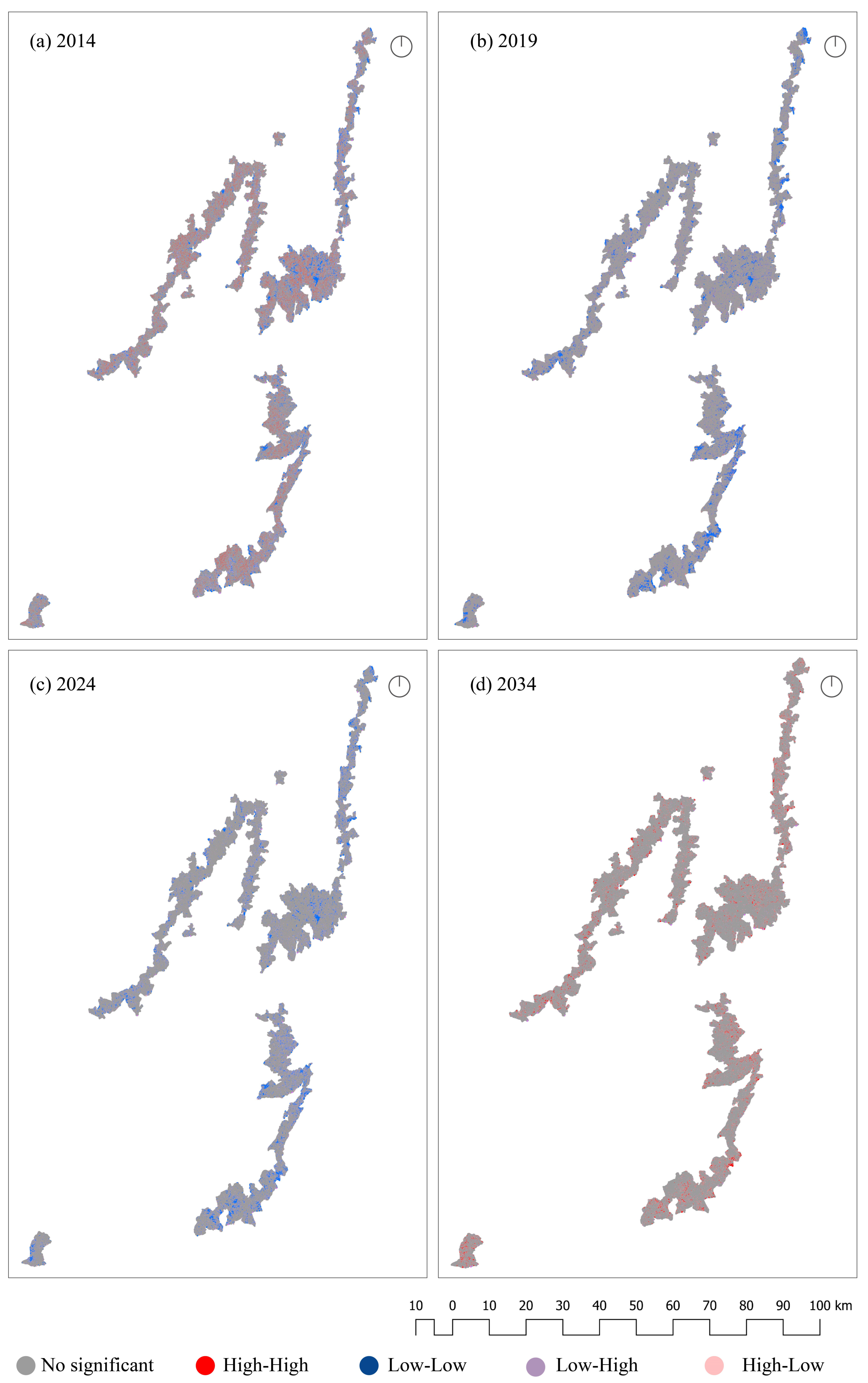
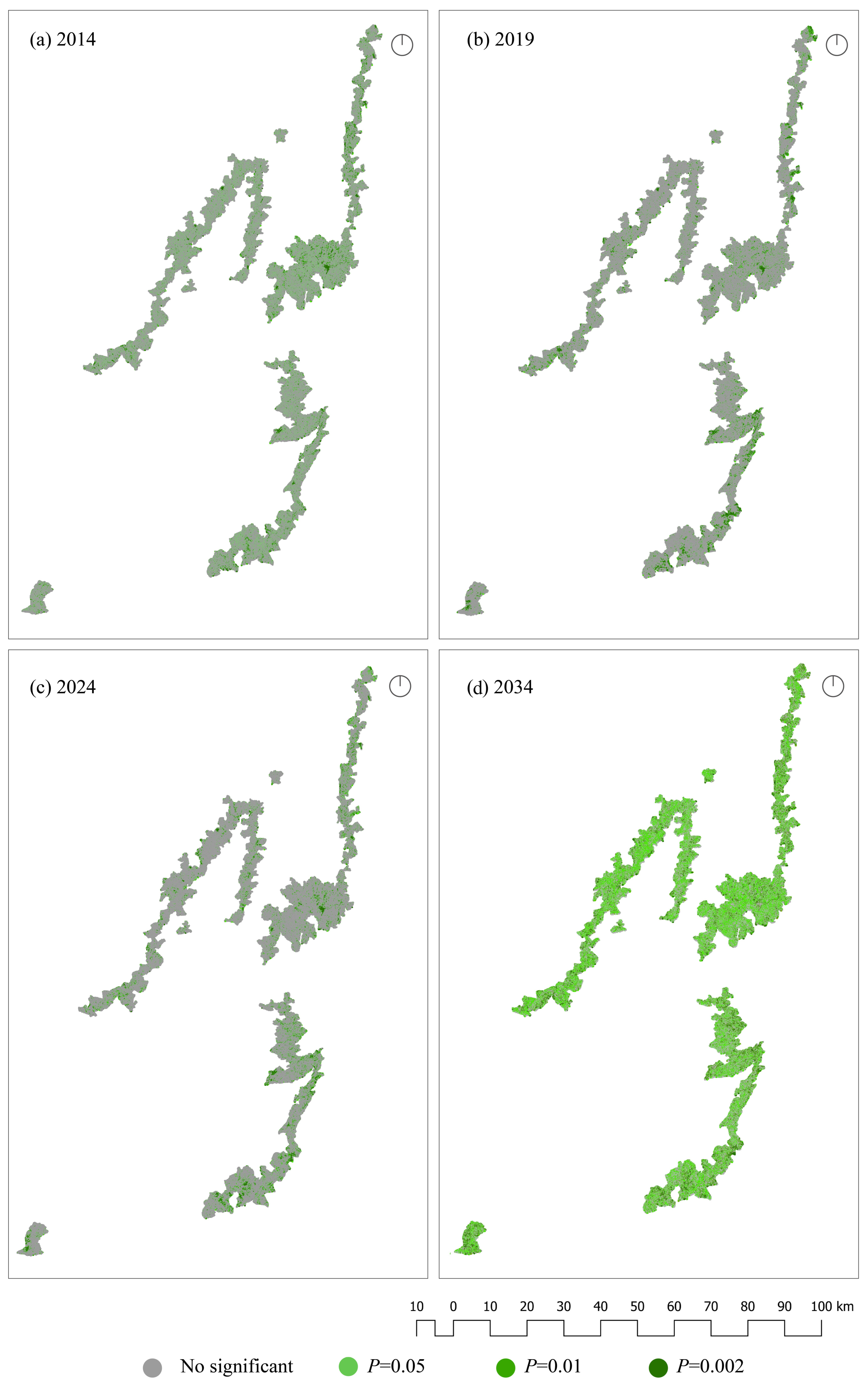
3.4.2. Local Autocorrelation Analysis

The local autocorrelation of the Land Use Degree Index (LUDI) in the CCLC was analyzed for the years 2014, 2019, 2024, and 2034 in order to identify changes in spatial distribution and assess their statistical significance in the autocorrelation patterns. For this purpose, Local Indicators of Spatial Association (LISA) were employed, which allowed for the detection of the spatiotemporal patterns of concentration and dispersion in land use. The results are presented in Figure 12 and Figure 13, offering a detailed view of the evolution and intensity of land occupation over the analysis period.
In 2014 and 2019, areas with “High–High” values were primarily concentrated in urban and intermediate zones, with significance levels predominantly ranging between 0.002 and 0.100, while “Low–Low” areas were associated with rural regions of low activity, exhibiting similar significance levels.
For 2024, “High–High” clusters reached their greatest expansion, reflecting an intensification of land use in peri-urban areas, whereas “Low–Low” clusters began to disperse, with significance values ranging between 0.100 and 0.244, indicating spatial heterogeneity.
In 2034, “High–High” clusters experienced a contraction in some urban areas, although they maintained high significance levels (0.002–0.100). On the other hand, “Low–Low” areas consolidated in marginal rural regions, achieving greater stability and spatial homogenization.

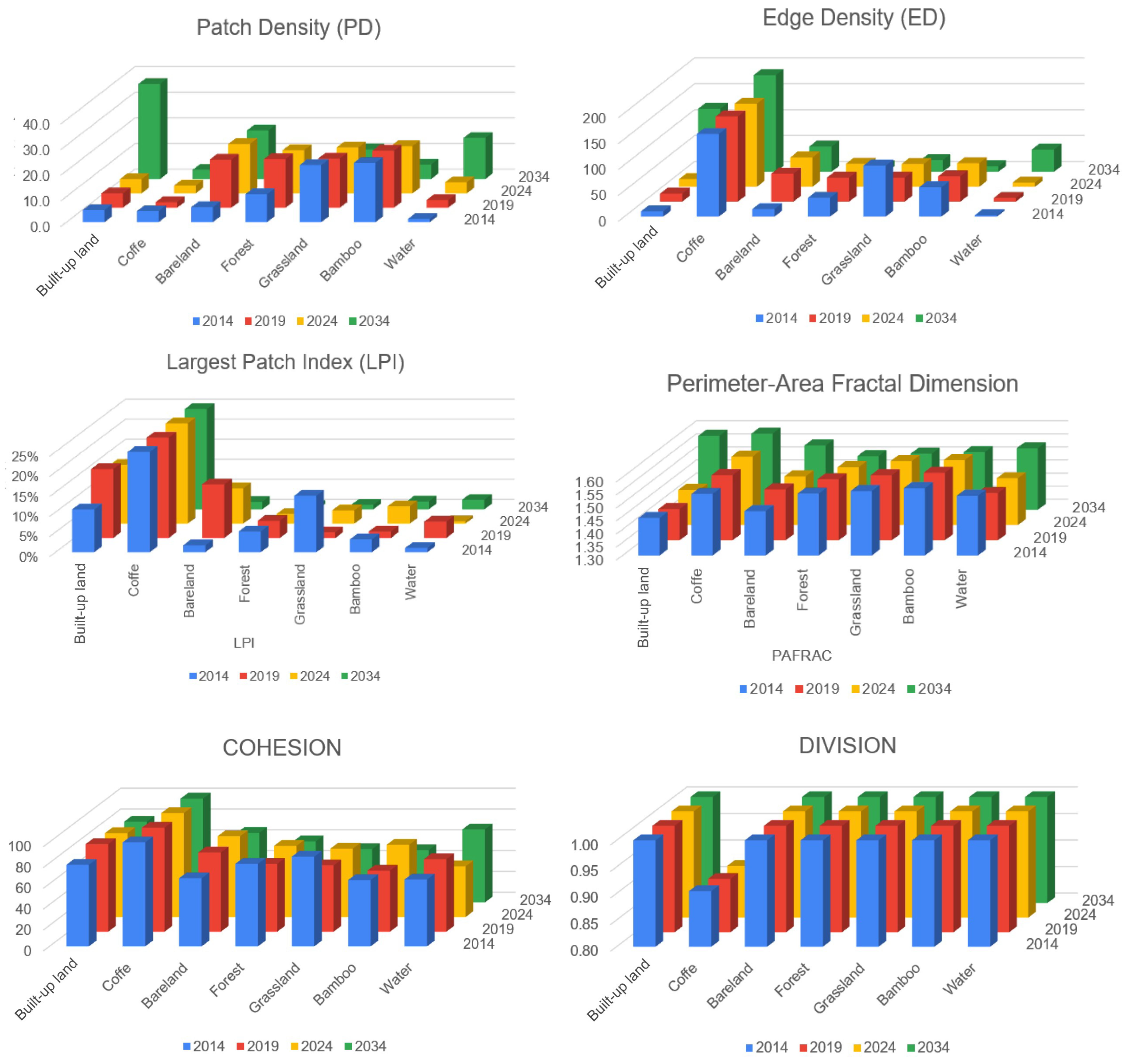
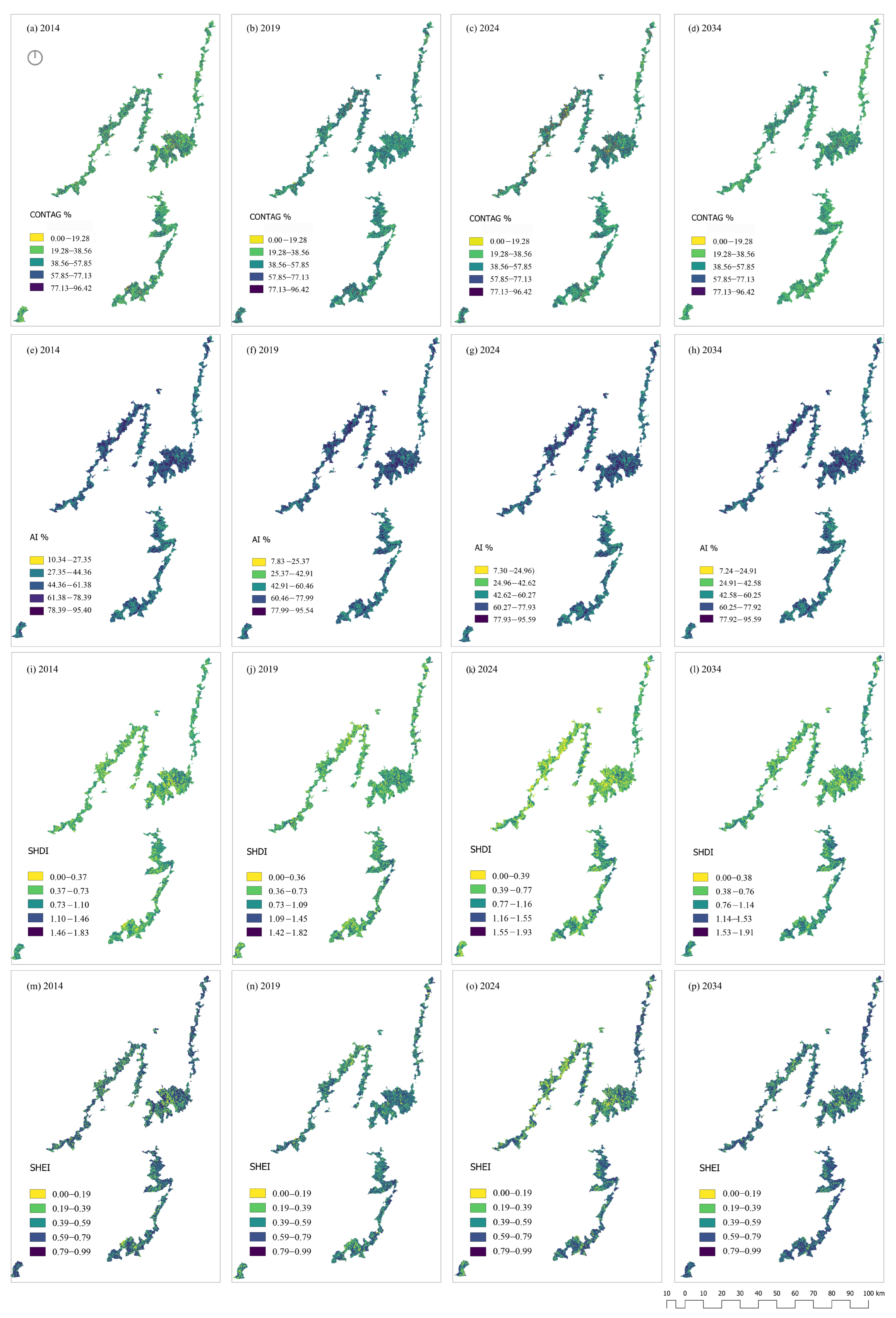
3.5. Spatiotemporal Characteristics of Landscape Patterns

The period 2014–2034 reveals a growing trend toward fragmentation in the CCLC, with differentiated spatial behaviors among land cover types. At the class level, the patch density index (PD) exhibits a significant increase in built-up land, rising from 4.7 in 2014 to 37.1 in 2034, indicating an accelerated urbanization process. In contrast, coffee crops show a slight decrease (from 4.3 to 3.7), and natural covers such as forests and grasslands demonstrate a marked reduction (from 10.9 to 4.9 and 22.2 to 11.6, respectively), suggesting consolidation. Bareland increases substantially (from 5.8 to 19.0), while bamboo and water bodies reflect divergent trends, with bamboo decreasing from 23.1 to 5.7 and water increasing from 1.3 to 16.1, suggesting the greater fragmentation or proliferation of aquatic features.
The edge density index (ED) also presents notable changes. Coffee crops increase in internal fragmentation (from 159.48 to 186.8), while forest cover shows simplification (from 36.36 to 10.8). Built-up land increases sharply in edge complexity (from 10.25 to 121.7), and bareland and water bodies also reflect this trend. In contrast, grasslands and bamboo decrease notably in edge complexity. The trends in PD and ED are illustrated in Figure 14.
The Largest Patch Index (LPI) shows that coffee crops maintain stable dominance with a minor decline (from 21.84 to 21.79), while forest, grasslands, and bamboo decrease markedly, indicating the loss of dominant continuous patches. Bareland and water maintain low values, and built-up land remains constant at 0.11, highlighting the dispersed urban growth.
The Perimeter-Area Fractal Dimension (PAFRAC) reflects increasing complexity in urban patches (from 1.44 to 1.5834) and moderate complexity in coffee crops and bareland. Conversely, natural covers (forest, grasslands, bamboo) show a slight simplification of patch shapes, while water bodies increase slightly in complexity.
The COHESION index illustrates contrasting connectivity patterns. Built-up land remains relatively stable (from 78.21 to 77.64), while coffee crops maintain high cohesion (~99.83). Forest and grasslands undergo fragmentation (falling from 79.16 to 58.74 and 86.04 to 51.19, respectively), and bamboo also declines (from 63.60 to 50.20). Interestingly, water bodies increase in cohesion (from 64.10 to 70.17), possibly due to the expansion or interconnection of aquatic patches.
The DIVISION index shows a slight increase in fragmentation for coffee crops (from 0.90 to 0.908), while all other covers—including built-up land, bareland, forest, grasslands, bamboo, and water—maintain a value of 1.00, indicating a consistently high level of spatial separation and low internal cohesion.
At the landscape level, broader patterns are evident. The Contagion Index (CONTAG) increases in 2019 and 2024 compared to 2014, suggesting more aggregated land cover configurations. However, in 2034, the decrease in CONTAG values reflects a fragmented landscape structure, primarily driven by urban expansion. The spatial maps show greater clustering of natural covers in 2019–2024, and more dispersion by 2034, especially in the central areas of the territory.
The Aggregation Index (AI) further supports this, with the minimum values declining from 10.34 in 2014 to 7.24 in 2034, particularly in the central zones affected by urban development. In contrast, the maximum AI values remain stable (between 95.40 and 95.59), especially in the northern and southern rural areas dominated by forest and water.
The Shannon Diversity Index (SHDI) and Shannon Evenness Index (SHEI) show that zones with high diversity and balanced distribution are consistently located in the central and southern regions, while the north remains more homogeneous. Over time, the increase in SHDI and SHEI values reflects greater heterogeneity in land composition and spatial distribution. These trends are illustrated in Figure 15, which shows the spatial configuration of CONTAG, AI, SHDI, and SHEI in 2034. This pattern, shaped by mountainous topography and urban development, emphasizes the progressive fragmentation and decline of ecological connectivity in the CCLC.

4. Discussion

4.1. Land Use and Land Cover Transformations

The dynamics of land use observed in the CCLC between 2014 and 2034 reflect transformations aligned with global trends in cultural landscapes [106,107,108]. The findings indicate an increasingly anthropized scenario, characterized by rapid urban expansion from 1.48% in 2014 to 15.64% in 2034, a projected 77.8% decline in forest cover by 2034, and a gradual reduction in coffee cultivation by 1% over two decades. These dynamics mirror patterns observed in cultural and heritage agricultural landscapes worldwide, where socioeconomic and demographic pressures drive rapid land use changes, threatening their ecological and cultural integrity [16,20].
Urbanization, the main driver of change, is associated with population growth, increased housing demand—including peri-urban expansion, second homes, and tourism infrastructure—as well as the limited containment capacity of the current legislative framework [109]. This pattern is consistent with processes documented in heritage landscapes such as Cairo in Egypt and Nansha in China [110,111]. In the case of the CCLC, such transformation poses a risk to the preservation of its Outstanding Universal Value. Although coffee cultivation is expected to maintain its coverage by 2034, it exhibits gradual fluctuations that compromise the productive and cultural foundation of the territory. Factors such as the low profitability of traditional coffee farming, the aging of the rural population, and the absence of generational renewal explain this trend, which has already been observed in other heritage agricultural landscapes such as the rice terraces in the Philippines [112], where many plots have been abandoned or repurposed.
Simultaneously, the reduction in grasslands (from 15.7% to 5.83%) and the increase in bareland (from 1.83% to 2.33%) indicate an intensification and reconfiguration of land use, due to temporary abandonment, site preparation for new developments, or transitions toward urban uses. The projected loss of more than 77.8% of forest cover, although requiring further detailed analysis, raises concerns about the severe impacts on biodiversity and ecosystem services. This trend is consistent with the critical deforestation rates reported in other South American landscapes [113], underscoring the intense anthropogenic pressure on both ecological and cultural values within the CCLC. Notably, forest cover experiences a temporary increase between 2019 and 2024, which may be partially attributed to reduced anthropogenic activity during the COVID-19 pandemic, likely slowing land conversion processes [114]. However, this short-term recovery appears to be an anomaly, as model projections indicate a substantial reversal: a 79.55% relative loss of forest cover between 2024 and 2034. This anticipated decline highlights the persistent influence of urban expansion and suggests that the long-term reduction in forest extent—amounting to a 77.80% overall loss since 2014—is primarily driven by direct deforestation rather than gradual landscape transformation alone.

4.2. Ecological Fragmentation and Spatial Landscape Patterns

Between 2014 and 2034, the analysis of landscape metrics reveals increasing fragmentation and spatial heterogeneity in the CCLC, driven by urbanization and land use intensification. The 25% increase in the number of patches and the 23.6% rise in edge density indicate greater territorial subdivision. The decline in the Contagion Index (CONTAG) and the rise in the Shannon Diversity Index (SHDI) reflect a more heterogeneous and less connected landscape, where diverse land uses replace continuous covers such as coffee plantations. The decrease in Moran’s I index (from 0.39 to 0.33) suggests reduced spatial cohesion, while the LISA analysis identifies transformation hotspots in urban peripheries, where land conversion is concentrated. This loss of connectivity affects species mobility and the flow of ecosystem services, mirroring the patterns observed in other rural landscapes undergoing transition [115]. Projections for 2034, with urban expansion reaching 17% and coffee cultivation decreasing to 62%, indicate territorial restructuring. The Land Use Degree Index (LUDI) supports this trend: higher values are associated with urban zones, while lower values correspond to persistent covers such as water bodies. This transformation resembles the processes observed in the Yayo Biosphere Reserve in Ethiopia [116], another coffee-producing landscape where a combination of agricultural expansion and population growth has led to drastic landscape reorganization and a loss of ecological connectivity.

4.3. Persistence of the Coffee Landscape and Resilience Processes

Despite territorial pressures, the CCLC demonstrates resilience through the continuity of coffee cultivation and traditional practices. It is important to note that urban expansion does not necessarily entail degradation, as in some cases it improves access to infrastructure and services, generating social benefits. This dynamic presents inherent trade-offs, particularly within a valued cultural landscape where development pressures must be carefully weighed against heritage conservation. Effectively navigating these transformations requires acknowledging both potential socioeconomic gains and the impacts on the landscape’s integrity. The coexistence of transformation processes and adaptation strategies confirms the active character of the CCLC as a living landscape.
Local initiatives such as shade-grown coffee, specialty coffee production, rural tourism, and community organization—developed in municipalities such as Filandia, Salento, and Salamina [109]—enhance the response to land use change. Although these actions are not directly captured through remote sensing results, they contribute to maintaining the ecological and functional heterogeneity of the territory.
Similar trajectories are observed in other traditional landscapes recognized by UNESCO [111,116], where urbanization, shifts in agricultural practices, and habitat loss represent common challenges. In this context, the future of the CCLC will depend on the capacity of its stakeholders to manage land use conflicts and strengthen sustainable practices. While the 2034 projection warns of potentially undesirable trajectories, it also helps identify priority areas for intervention.

4.4. Study Limitations and Future Research Directions

This study provides relevant findings; however, it is essential to acknowledge its limitations and suggest potential avenues for future research. First, the predictive model is based on a Business as Usual scenario that does not account for the implementation of the protection policies promoted by UNESCO [117]. This choice is justified by the limited application of land use planning instruments in the municipalities analyzed and by the gaps in the enforcement of existing regulations. However, future models could incorporate policy-based scenarios aligned with UNESCO guidelines, allowing the simulation of land use changes under conservation-oriented constraints [109,114]. As a result, the model does not include alternative scenarios for urban containment.
Second, the analysis is restricted to the core zone of the Colombian Coffee Cultural Landscape, following the heritage integrity criteria defined by UNESCO [30]. This decision, while methodologically justified, also implies a trade-off. Focusing solely on the core zone ensures analytical precision and alignment with UNESCO’s definition of the inscribed property, but it limits the capacity to evaluate indirect transformations occurring in the buffer zone, such as fringe urbanization or landscape fragmentation beyond the core boundary. Third, the ecological projections do not incorporate field data on biodiversity or ecosystem services, which restricts the functional interpretation of landscape fragmentation. Integrating empirical data would strengthen the link between spatial patterns and ecological processes.
In addition, the 30 m spatial resolution may limit the detection of localized urban expansion, especially in areas characterized by small-scale or informal development. Subpixel urban changes may remain undetected, potentially affecting the accuracy of urban growth projections in densely built environments.

5. Conclusions

This study integrated multisensor remote sensing, hybrid predictive CA-ANN models, and a detailed analysis of landscape metrics to evaluate the evolution of LULC and the impacts of landscape patterns in the Coffee Cultural Landscape of Colombia (CCLC) during the period 2014–2034. The results demonstrate significant changes in the landscape structure driven by territorial transformation and anthropogenic pressures. The main conclusions are as follows:
LULC Dynamics and Spatial Trends: An accelerated expansion of built-up land was observed, increasing from a marginal share in 2014 to a drastic projected presence in 2034. This trend reflected a pattern of disorderly urbanization that posed risks to the integrity of the natural landscape. Although coffee crops remained the dominant land cover, they were projected to decline, signaling mounting pressure on traditional productive areas due to land use conversion.
Impact on Landscape Structure and Fragmentation: Forests and other natural ecosystems exhibited a marked reduction over the study period. The simultaneous increase in built-up land contributed to the heightened fragmentation and heterogeneity of the landscape. The metrics revealed greater patch dispersion and complexity, indicating a loss of connectivity and reduced ecological stability.
Methodological Efficacy and Planning Relevance: The combination of optical and radar data, the Random Forest classification algorithm, and CA-ANN modeling yielded high accuracy, validating the robustness of the proposed approach. The quantitative analysis of landscape metrics proved valuable for identifying risk areas and guiding conservation and mitigation strategies under increasing socio-environmental pressure.
Trade-offs and Balanced Landscape Management: While the findings highlighted potential ecological and cultural threats—especially from uncontrolled urbanization and the decline of traditional productive landscapes—they also revealed opportunities. Managed urban development can bring socioeconomic benefits such as improved infrastructure, accessibility, and quality of life for local communities. Recognizing these trade-offs is crucial for effective planning. Sustainable territorial governance must balance the preservation of ecosystems and cultural heritage (which underpin the CCLC’s Outstanding Universal Value) with the development needs of its inhabitants.
This study provides a robust scientific and methodological foundation for understanding LULC transitions and landscape dynamics in heritage regions. The conclusions serve as a critical reference to inform territorial decision-making, offering actionable insights to mitigate negative impacts while promoting ecological resilience and inclusive, adaptive land management in this valuable cultural landscape.

Supplementary Materials

The following supporting information can be downloaded at: https://www.mdpi.com/article/10.3390/land14051045/s1.

Author Contributions

Conceptualization, A.P.R.C.; methodology, A.P.R.C. and J.S.; software, A.P.R.C. and J.D.M.O.; validation, A.P.R.C., J.S. and J.D.M.O.; formal analysis, A.P.R.C. and J.D.M.O.; investigation, A.P.R.C.; resources, A.P.R.C.; data curation, A.P.R.C.; writing—original draft preparation, A.P.R.C.; writing—review and editing, A.P.R.C. and J.D.M.O.; visualization, A.P.R.C. and J.D.M.O.; supervision, J.S.; project administration, J.S.; funding acquisition, A.P.R.C. All authors have read and agreed to the published version of the manuscript.

Funding

This research was funded by the Center for Balance Architecture, Zhejiang University, grant number K-20212936.

Informed Consent Statement

Informed consent was obtained from all subjects involved in the study.

Data Availability Statement

The original contributions presented in this study are included in the article/Supplementary Materials. Further inquiries can be directed to the corresponding author.

Acknowledgments

We would like to acknowledge the support from Center for Balance Architecture, Zhejiang University.

Conflicts of Interest

The authors declare no conflicts of interest.

Appendix A

The described procedure was implemented using a script in Google Earth Engine (GEE), available at: https://code.earthengine.google.com/be158215b47827977de85525784ae34f (accessed on 8 September 2024).

Appendix B

Table A1 describes the indices used to assess fragmentation, connectivity, and landscape structure in the study. Each metric is presented with its equation, variables, and interpretive meaning.
Table A1. Indices and their meanings for landscape patterns.
ScaleIndex and EquationVariable DeclarationMeaning
Class
metrics
P D   =   N   /   A PD: Patch density
N is the number of patches
A is the area of a certain
type of landscape
PD reflects the degree of landscape fragmentation within a certain area. The greater the patch density, the greater the degree of fragmentation.
E D = i = 1 M j = 1 M P i j A ED: Edge density Pᵢⱼ: Edge length between patch i and
patch j M: Total number
of patch classes in the
landscape A: Total landscape area
ED reflects the edge length between the patches of heterogeneous landscape elements per unit area within a certain regional landscape scope.
L P I = m a x ( a i ) A   × 100 LPI: Largest Patch Index
max (aᵢ): Area of the largest
patch in class i A: Total landscape area ×100: converts the result to a percentage
LPI is the percentage of the largest patch area in the total landscape area, and is a measure of the dominance degree at the patch level.
P A F R A C = 2 ln A ln P i j ln a i j Pij: Perimeter of patch ij aij: Area of patch ij A: Total landscape areaPAFRAC reflects the degree of disturbance from human activities in the landscape pattern, but the formula should be carefully verified for accuracy.
C O H = 1 i = 1 n P i i = 1 n A i 1 1 A 1 100 Pi: Perimeter of patch i Ai: Area of patch I A: Total landscape area n: Total number of patches in the class or landscapeCOHESION reflects the aggregation and dispersion of landscape elements.
Landscape metrics D I V I S I O N = 1 i = 1 n a i j A 2 aij: Area of patch ij A: Total landscape area n: Total number of patchesDIVISION reflects the degree of fragmentation of patches within the region.
A I = g i i g i i m a x × 100 gii: Number of like adjacencies between pixels of class I giimax: Maximum possible number of like adjacencies for class iAI reflects the degree of patch aggregation in the landscape. A higher value indicates greater aggregation.
C O N T A G = 1 + i = 1 m j = 1 m P i j P i j ln P i j P i j 2 ln m × 100 Pij: Proportion of adjacencies between patch types i and j m: Total number of patch types (classes) in the landscape ∑Pij: Total number of pairwise adjacencies in the landscapeCONTAG measures the degree of aggregation of different patch types in a given area. A higher value indicates greater aggregation.
S H D I = i = 1 m P i ln P i Pi: Proportion of the landscape occupied by patch type I m: Total number of patch types in the landscape ln: Natural logarithmSHDI reflects the diversity of landscape elements in a given area. A higher value indicates greater diversity.
S H E I = S H D I ln m SHEI: Shannon’s Evenness Index SHDI: Shannon Diversity Index
m: Total number of patch types in the landscape
SHEI measures the evenness in the distribution of patch types. A higher value indicates a more even distribution.

References

  1. Badman, T.; Bomhard, B.; Fincke, A.; Langley, J.; Rosabal, P.; Sheppard, D. Outstanding Universal Value: Standards for Natural World Heritage; IUCN: Gland, Switzerland, 2008. [Google Scholar]
  2. Guo, H.; Chen, F.; Tang, Y.; Ding, Y.; Chen, M.; Zhou, W.; Zhu, M.; Gao, S.; Yang, R.; Zheng, W.; et al. Progress toward the Sustainable Development of World Cultural Heritage Sites Facing Land-Cover Changes. Innovation 2023, 4, 100496. [Google Scholar] [CrossRef] [PubMed]
  3. Winkler, K.; Fuchs, R.; Rounsevell, M.; Herold, M. Global Land Use Changes Are Four Times Greater than Previously Estimated. Nat. Commun. 2021, 12, 2501. [Google Scholar] [CrossRef] [PubMed]
  4. He, D.; Chen, W.; Zhang, J. Integrating Heritage and Environment: Characterization of Cultural Landscape in Beijing Great Wall Heritage Area. Land 2024, 13, 536. [Google Scholar] [CrossRef]
  5. Venter, O.; Sanderson, E.W.; Magrach, A.; Allan, J.R.; Beher, J.; Jones, K.R.; Possingham, H.P.; Laurance, W.F.; Wood, P.; Fekete, B.M.; et al. Sixteen Years of Change in the Global Terrestrial Human Footprint and Implications for Biodiversity Conservation. Nat. Commun. 2016, 7, 12558. [Google Scholar] [CrossRef]
  6. Garrard, R.; Kohler, T.; Price, M.F.; Byers, A.C.; Sherpa, A.R.; Maharjan, G.R. Land Use and Land Cover Change in Sagarmatha National Park, a World Heritage Site in the Himalayas of Eastern Nepal. Mt. Res. Dev. 2016, 36, 299. [Google Scholar] [CrossRef]
  7. Kim, J.; Choi, H.; Shin, W.; Yun, J.; Song, Y. Complex Spatiotemporal Changes in Land-Use and Ecosystem Services in the Jeju Island UNESCO Heritage and Biosphere Site (Republic of Korea). Environ. Conserv. 2022, 49, 272–279. [Google Scholar] [CrossRef]
  8. Remond-Noa, R.; González-Sousa, R.; Cámara-García, F.L.; Cabrera, N.; Quintana-Cortina, C.; Martínez-Murillo, J.F. Modelling Land Use Changes and Impacts on the Visual Fragility of a UNESCO Landscape Heritage Site (Viñales, Cuba). In Mapping and Forecasting Land Use; Elsevier: Amsterdam, The Netherlands, 2022; pp. 265–297. ISBN 978-0-323-90947-1. [Google Scholar]
  9. Lambin, E.F.; Geist, H.J.; Lepers, E. Dynamics of Land-Use and Land-Cover Change in Tropical Regions. Annu. Rev. Environ. Resour. 2003, 28, 205–241. [Google Scholar] [CrossRef]
  10. Palang, H.; Soini, K.; Printsmann, A.; Birkeland, I. Landscape and Cultural Sustainability. Nor. Geogr. Tidsskr. Nor. J. Geogr. 2017, 71, 127–131. [Google Scholar] [CrossRef]
  11. Zimmermann, P.; Tasser, E.; Leitinger, G.; Tappeiner, U. Effects of Land-Use and Land-Cover Pattern on Landscape-Scale Biodiversity in the European Alps. Agric. Ecosyst. Environ. 2010, 139, 13–22. [Google Scholar] [CrossRef]
  12. Zhao, Q.; Wen, Z.; Chen, S.; Ding, S.; Zhang, M. Quantifying Land Use/Land Cover and Landscape Pattern Changes and Impacts on Ecosystem Services. Int. J. Environ. Res. Public Health 2020, 17, 126. [Google Scholar] [CrossRef]
  13. Foley, J.A.; DeFries, R.; Asner, G.P.; Barford, C.; Bonan, G.; Carpenter, S.R.; Chapin, F.S.; Coe, M.T.; Daily, G.C.; Gibbs, H.K.; et al. Global Consequences of Land Use. Science 2005, 309, 570–574. [Google Scholar] [CrossRef]
  14. Medeiros, A.; Fernandes, C.; Gonçalves, J.F.; Farinha-Marques, P. A Diagnostic Framework for Assessing Land-Use Change Impacts on Landscape Pattern and Character—A Case-Study from the Douro Region, Portugal. Landsc. Urban Plan. 2022, 228, 104580. [Google Scholar] [CrossRef]
  15. Li, X.; Yeh, A.G.-O. Analyzing Spatial Restructuring of Land Use Patterns in a Fast Growing Region Using Remote Sensing and GIS. Landsc. Urban Plan. 2004, 69, 335–354. [Google Scholar] [CrossRef]
  16. Ren, S.; Zhao, H.; Zhang, H.; Wang, F.; Yang, H. Influence of Natural and Social Economic Factors on Landscape Pattern Indices—The Case of the Yellow River Basin in Henan Province. Water 2023, 15, 4174. [Google Scholar] [CrossRef]
  17. Demessie, S.F.; Dile, Y.T.; Bedadi, B.; Tarkegn, T.G.; Bayabil, H.K.; Sintayehu, D.W. Assessing and Projecting Land Use Land Cover Changes Using Machine Learning Models in the Guder Watershed, Ethiopia. Environ. Chall. 2025, 18, 101074. [Google Scholar] [CrossRef]
  18. Murillo-López, B.E.; Feijoo-Martínez, A.; Carvajal, A.F. Land Cover Changes in Coffee Cultural Landscapes of Pereira (Colombia) between 1997 and 2014. Cuad. Investig. Geogr. 2022, 48, 175–196. [Google Scholar] [CrossRef]
  19. Wang, Q.; Bai, X. Spatiotemporal Characteristics and Driving Mechanisms of Land-Use Transitions and Landscape Patterns in Response to Ecological Restoration Projects: A Case Study of Mountainous Areas in Guizhou, Southwest China. Ecol. Inform. 2024, 82, 102748. [Google Scholar] [CrossRef]
  20. Wang, Q.; Wang, H. Spatiotemporal Dynamics and Evolution Relationships between Land-Use/Land Cover Change and Landscape Pattern in Response to Rapid Urban Sprawl Process: A Case Study in Wuhan, China. Ecol. Eng. 2022, 182, 106716. [Google Scholar] [CrossRef]
  21. Chaves, M.E.D.; Picoli, M.C.A.; Sanches, I.D. Recent Applications of Landsat 8/OLI and Sentinel-2/MSI for Land Use and Land Cover Mapping: A Systematic Review. Remote Sens. 2020, 12, 3062. [Google Scholar] [CrossRef]
  22. Hunt, D.A.; Tabor, K.; Hewson, J.H.; Wood, M.A.; Reymondin, L.; Koenig, K.; Schmitt-Harsh, M.; Follett, F. Review of Remote Sensing Methods to Map Coffee Production Systems. Remote Sens. 2020, 12, 2041. [Google Scholar] [CrossRef]
  23. Kamaraj, M.; Rangarajan, S. Predicting the Future Land Use and Land Cover Changes for Bhavani Basin, Tamil Nadu, India Using QGIS MOLUSCE Plugin. Environ. Sci. Pollut. Res. 2021, 29, 86337–86348. [Google Scholar] [CrossRef] [PubMed]
  24. Cruz-Rincón, D.F. Transformaciones, Contradicciones y Paradojas Del Paisaje Cultural Cafetero de Colombia: Una Revisión de Literatura. Soc. Econ. 2024, 51, e10112226. [Google Scholar] [CrossRef]
  25. Coffee Cultural Landscape of Colombia—UNESCO World Heritage Centre. Available online: https://whc.unesco.org/en/list/1121 (accessed on 6 February 2025).
  26. Velandia Silva, C.; Arango, G.; Rivas, L.; Castañeda-Pérez, Y. Paisaje Cultural Cafetero: Excepcional Fusión Entre Naturaleza, Cultura y Trabajo Colectivo. (Editor) Versión Abreviada y Actualizada 2016; Federación Nacional de Cafeteros de Colombia: Armenia, Colombia, 2016; ISBN 978-958-56007-0-6. [Google Scholar]
  27. Etter, A.; McAlpine, C.; Wilson, K.; Phinn, S.; Possingham, H. Regional Patterns of Agricultural Land Use and Deforestation in Colombia. Agric. Ecosyst. Environ. 2006, 114, 369–386. [Google Scholar] [CrossRef]
  28. Cifuentes Monsalve, D.M.; Duque Arango, G.I. La Transformación Del Paisaje Urbano Rural Del Municipio de Montenegro, Quindío. MÓDULO Arquit. CUC 2021, 26, 191–216. [Google Scholar] [CrossRef]
  29. Murillo-López, B.E.; Castro, A.J.; Feijoo-Martínez, A. Nature’s Contributions to People Shape Sense of Place in the Coffee Cultural Landscape of Colombia. Agriculture 2022, 12, 457. [Google Scholar] [CrossRef]
  30. UNESCO World Heritage Centre. Note 1—Identifying and Mapping Attributes That Convey the Outstanding Universal Value of a World Heritage Property. Available online: https://whc.unesco.org/en/wind-energy/note1/ (accessed on 8 April 2025).
  31. UNESCO World Heritage Centre—Compendium. Available online: https://whc.unesco.org/en/compendium/?action=list&id_faq_themes=972,1526,1528,1530,1532 (accessed on 8 April 2025).
  32. UNESCO World Heritage Centre. Buffer Zones—Glossary. Available online: https://whc.unesco.org/en/glossary/199 (accessed on 8 April 2025).
  33. Inglada, J.; Vincent, A.; Arias, M.; Marais-Sicre, C. Improved Early Crop Type Identification By Joint Use of High Temporal Resolution SAR And Optical Image Time Series. Remote Sens. 2016, 8, 362. [Google Scholar] [CrossRef]
  34. Kussul, N.; Lemoine, G.; Gallego, F.J.; Skakun, S.V.; Lavreniuk, M.; Shelestov, A.Y. Parcel-Based Crop Classification in Ukraine Using Landsat-8 Data and Sentinel-1A Data. IEEE J. Sel. Top. Appl. Earth Obs. Remote Sens. 2016, 9, 2500–2508. [Google Scholar] [CrossRef]
  35. DeVries, B.; Huang, C.; Armston, J.; Huang, W.; Jones, J.W.; Lang, M.W. Rapid and Robust Monitoring of Flood Events Using Sentinel-1 and Landsat Data on the Google Earth Engine. Remote Sens. Environ. 2020, 240, 111664. [Google Scholar] [CrossRef]
  36. Chander, G.; Markham, B.L.; Helder, D.L. Summary of Current Radiometric Calibration Coefficients for Landsat MSS, TM, ETM+, and EO-1 ALI Sensors. Remote Sens. Environ. 2009, 113, 893–903. [Google Scholar] [CrossRef]
  37. Automated cloud, cloud shadow, and snow detection in multitemporal Landsat data: An algorithm designed specifically for monitoring land cover change. Remote Sens. Environ. 2014, 152, 217–234. [CrossRef]
  38. Mateo-García, G.; Gómez-Chova, L.; Amorós-López, J.; Muñoz-Marí, J.; Camps-Valls, G. Multitemporal Cloud Masking in the Google Earth Engine. Remote Sens. 2018, 10, 1079. [Google Scholar] [CrossRef]
  39. Gorelick, N.; Hancher, M.; Dixon, M.; Ilyushchenko, S.; Thau, D.; Moore, R. Google Earth Engine: Planetary-Scale Geospatial Analysis for Everyone. Remote Sens. Environ. 2017, 202, 18–27. [Google Scholar] [CrossRef]
  40. Dos Santos, E.P.; Da Silva, D.D.; Do Amaral, C.H.; Fernandes-Filho, E.I.; Dias, R.L.S. A Machine Learning Approach to Reconstruct Cloudy Affected Vegetation Indices Imagery via Data Fusion from Sentinel-1 and Landsat 8. Comput. Electron. Agric. 2022, 194, 106753. [Google Scholar] [CrossRef]
  41. Zhang, Z.; Wei, M.; Pu, D.; He, G.; Wang, G.; Long, T. Assessment of Annual Composite Images Obtained by Google Earth Engine for Urban Areas Mapping Using Random Forest. Remote Sens. 2021, 13, 748. [Google Scholar] [CrossRef]
  42. White, J.C.; Wulder, M.A.; Hobart, G.W.; Luther, J.E.; Hermosilla, T.; Griffiths, P.; Coops, N.C.; Hall, R.J.; Hostert, P.; Dyk, A.; et al. Pixel-Based Image Compositing for Large-Area Dense Time Series Applications and Science. Can. J. Remote Sens. 2014, 40, 192–212. [Google Scholar] [CrossRef]
  43. Torres, R.; Snoeij, P.; Geudtner, D.; Bibby, D.; Davidson, M.; Attema, E.; Potin, P.; Rommen, B.; Floury, N.; Brown, M.; et al. GMES Sentinel-1 Mission. Remote Sens. Environ. 2012, 120, 9–24. [Google Scholar] [CrossRef]
  44. Dostálová, A.; Hollaus, M.; Milenković, M.; Wagner, W. FOREST AREA DERIVATION FROM SENTINEL-1 DATA. ISPRS Ann. Photogramm. Remote Sens. Spat. Inf. Sci. 2016, III–7, 227–233. [Google Scholar] [CrossRef]
  45. Sánchez-Méndez, A.G.; Arguijo-Hernández, S.P. Análisis de imágenes multiespectrales para la detección de cultivos y detección de plagas y enfermedades en la producción de café. Res. Comput. Sci. 2018, 147, 309–317. [Google Scholar] [CrossRef]
  46. Chemura, A.; Mutanga, O.; Dube, T. Integrating Age in the Detection and Mapping of Incongruous Patches in Coffee (Coffea Arabica) Plantations Using Multi-Temporal Landsat 8 NDVI Anomalies. Int. J. Appl. Earth Obs. Geoinform. 2017, 57, 1–13. [Google Scholar] [CrossRef]
  47. Roy, D.P.; Wulder, M.A.; Loveland, T.R.; Woodcock, C.E.; Allen, R.G.; Anderson, M.C.; Helder, D.; Irons, J.R.; Johnson, D.M.; Kennedy, R.; et al. Landsat-8: Science and Product Vision for Terrestrial Global Change Research. Remote Sens. Environ. 2014, 145, 154–172. [Google Scholar] [CrossRef]
  48. Vermote, E.; Justice, C.; Claverie, M.; Franch, B. Preliminary Analysis of the Performance of the Landsat 8/OLI Land Surface Reflectance Product. Remote Sens. Environ. 2016, 185, 46–56. [Google Scholar] [CrossRef] [PubMed]
  49. Feng, X.; Tan, S.; Dong, Y.; Zhang, X.; Xu, J.; Zhong, L.; Yu, L. Mapping Large-Scale Bamboo Forest Based on Phenology and Morphology Features. Remote Sens. 2023, 15, 515. [Google Scholar] [CrossRef]
  50. Fang, G.; Xu, H.; Yang, S.-I.; Lou, X.; Fang, L. Synergistic Use of Sentinel-1, Sentinel-2, and Landsat 8 in Predicting Forest Variables. Ecol. Indic. 2023, 151, 110296. [Google Scholar] [CrossRef]
  51. Jiang, Z.; Huete, A.; Didan, K.; Miura, T. Development of a Two-Band Enhanced Vegetation Index without a Blue Band. Remote Sens. Environ. 2008, 112, 3833–3845. [Google Scholar] [CrossRef]
  52. Saleska, S.R.; Wu, J.; Guan, K.; Araujo, A.C.; Huete, A.; Nobre, A.D.; Restrepo-Coupe, N. Dry-Season Greening of Amazon Forests. Nature 2016, 531, E4–E5. [Google Scholar] [CrossRef]
  53. Huete, A.R. A Soil-Adjusted Vegetation Index (SAVI). Remote Sens. Environ. 1988, 25, 295–309. [Google Scholar] [CrossRef]
  54. Escobar-López, A.; Castillo-Santiago, M.Á.; Mas, J.F.; Hernández-Stefanoni, J.L.; López-Martínez, J.O. Identification of Coffee Agroforestry Systems Using Remote Sensing Data: A Review of Methods and Sensor Data. Geocarto Int. 2024, 39, 2297555. [Google Scholar] [CrossRef]
  55. Ke, Y.; Im, J.; Lee, J.; Gong, H.; Ryu, Y. Characteristics of Landsat 8 OLI-Derived NDVI by Comparison with Multiple Satellite Sensors and in-Situ Observations. Remote Sens. Environ. 2015, 164, 298–313. [Google Scholar] [CrossRef]
  56. Wang, C.; Qi, S.; Niu, Z.; Wang, J. Evaluating Soil Moisture Status in China Using the Temperature–Vegetation Dryness Index (TVDI). Can. J. Remote Sens. 2004, 30, 671–679. [Google Scholar] [CrossRef]
  57. Susan Moran, M. Soil Moisture Evaluation Using Multi-Temporal Synthetic Aperture Radar (SAR) in Semiarid Rangeland. Agric. For. Meteorol. 2000, 105, 69–80. [Google Scholar] [CrossRef]
  58. Yang, Y.; Guan, H.; Long, D.; Liu, B.; Qin, G.; Qin, J.; Batelaan, O. Estimation of Surface Soil Moisture from Thermal Infrared Remote Sensing Using an Improved Trapezoid Method. Remote Sens. 2015, 7, 8250–8270. [Google Scholar] [CrossRef]
  59. Zha, Y.; Gao, J.; Ni, S. Use of Normalized Difference Built-up Index in Automatically Mapping Urban Areas from TM Imagery. Int. J. Remote Sens. 2003, 24, 583–594. [Google Scholar] [CrossRef]
  60. Muhaimin, M.; Fitriani, D.; Adyatma, S.; Arisanty, D. Mapping Build-up Area Density Using Normalized Difference Built-up Index (Ndbi) and Urban Index (Ui) Wetland in the City Banjarmasin. IOP Conf. Ser. Earth Environ. Sci. 2022, 1089, 012036. [Google Scholar] [CrossRef]
  61. Kawamura, M.; Jayamana, S.; Tsujiko, Y. Relation between Social and Environmental Conditions in Colombo Sri Lanka and the Urban Index Estimated by Satellite Remote Sensing Data. Int. Arch. Photogramm. Remote Sens. 1996, 31 (Pt B7), 321–326. [Google Scholar]
  62. Zhou, Y.; Yang, G.; Wang, S.; Wang, L.; Wang, F.; Liu, X. A New Index for Mapping Built-up and Bare Land Areas from Landsat-8 OLI Data. Remote Sens. Lett. 2014, 5, 862–871. [Google Scholar] [CrossRef]
  63. He, C.; Liu, Z.; Gou, S.; Zhang, Q.; Zhang, J.; Xu, L. Detecting Global Urban Expansion over the Last Three Decades Using a Fully Convolutional Network. Environ. Res. Lett. 2019, 14, 034008. [Google Scholar] [CrossRef]
  64. Diek, S.; Fornallaz, F.; Schaepman, M.E.; De Jong, R. Barest Pixel Composite for Agricultural Areas Using Landsat Time Series. Remote Sens. 2017, 9, 1245. [Google Scholar] [CrossRef]
  65. Wang, L.; Qu, J.J. Satellite Remote Sensing Applications for Surface Soil Moisture Monitoring: A Review. Front. Earth Sci. China 2009, 3, 237–247. [Google Scholar] [CrossRef]
  66. Xu, H. Modification of Normalised Difference Water Index (NDWI) to Enhance Open Water Features in Remotely Sensed Imagery. Int. J. Remote Sens. 2006, 27, 3025–3033. [Google Scholar] [CrossRef]
  67. Gao, B. NDWI—A Normalized Difference Water Index for Remote Sensing of Vegetation Liquid Water from Space. Remote Sens. Environ. 1996, 58, 257–266. [Google Scholar] [CrossRef]
  68. McFeeters, S.K. The Use of the Normalized Difference Water Index (NDWI) in the Delineation of Open Water Features. Int. J. Remote Sens. 1996, 17, 1425–1432. [Google Scholar] [CrossRef]
  69. Du, Y.; Zhang, Y.; Ling, F.; Wang, Q.; Li, W.; Li, X. Water Bodies’ Mapping from Sentinel-2 Imagery with Modified Normalized Difference Water Index at 10-m Spatial Resolution Produced by Sharpening the SWIR Band. Remote Sens. 2016, 8, 354. [Google Scholar] [CrossRef]
  70. Chandrasekar, K.; Sesha Sai, M.V.R.; Roy, P.S.; Dwevedi, R.S. Land Surface Water Index (LSWI) Response to Rainfall and NDVI Using the MODIS Vegetation Index Product. Int. J. Remote Sens. 2010, 31, 3987–4005. [Google Scholar] [CrossRef]
  71. Zhu, X.; Chen, J.; Gao, F.; Chen, X.; Masek, J.G. An Enhanced Spatial and Temporal Adaptive Reflectance Fusion Model for Complex Heterogeneous Regions. Remote Sens. Environ. 2010, 114, 2610–2623. [Google Scholar] [CrossRef]
  72. Congalton, R.G.; Green, K. Assessing the Accuracy of Remotely Sensed Data: Principles and Practices, 2nd ed.; CRC Press: Boca Raton, FL, USA, 2008; ISBN 978-0-429-14397-7. [Google Scholar]
  73. Shafizadeh-Moghadam, H.; Minaei, M.; Pontius, R.G., Jr.; Asghari, A.; Dadashpoor, H. Integrating a Forward Feature Selection Algorithm, Random Forest, and Cellular Automata to Extrapolate Urban Growth in the Tehran-Karaj Region of Iran. Comput. Environ. Urban Syst. 2021, 87, 101595. [Google Scholar] [CrossRef]
  74. Liu, Y.; Wang, Y.; Zhang, J. New Machine Learning Algorithm: Random Forest. In Proceedings of the Information Computing and Applications; Liu, B., Ma, M., Chang, J., Eds.; Springer: Berlin/Heidelberg, Germany, 2012; pp. 246–252. [Google Scholar]
  75. Sun, Z.; Wang, G.; Li, P.; Wang, H.; Zhang, M.; Liang, X. An Improved Random Forest Based on the Classification Accuracy and Correlation Measurement of Decision Trees. Expert Syst. Appl. 2024, 237, 121549. [Google Scholar] [CrossRef]
  76. Abbas, Z.; Jaber, H.S. Accuracy Assessment of Supervised Classification Methods for Extraction Land Use Maps Using Remote Sensing and GIS Techniques. IOP Conf. Ser. Mater. Sci. Eng. 2020, 745, 012166. [Google Scholar] [CrossRef]
  77. Amini, S.; Saber, M.; Rabiei-Dastjerdi, H.; Homayouni, S. Urban Land Use and Land Cover Change Analysis Using Random Forest Classification of Landsat Time Series. Remote Sens. 2022, 14, 2654. [Google Scholar] [CrossRef]
  78. Breiman, L. Random Forests. Mach. Learn. 2001, 45, 5–32. [Google Scholar] [CrossRef]
  79. Rodriguez-Galiano, V.F.; Ghimire, B.; Rogan, J.; Chica-Olmo, M.; Rigol-Sanchez, J.P. An Assessment of the Effectiveness of a Random Forest Classifier for Land-Cover Classification. ISPRS J. Photogramm. Remote Sens. 2012, 67, 93–104. [Google Scholar] [CrossRef]
  80. Olofsson, P.; Foody, G.M.; Herold, M.; Stehman, S.V.; Woodcock, C.E.; Wulder, M.A. Good Practices for Estimating Area and Assessing Accuracy of Land Change. Remote Sens. Environ. 2014, 148, 42–57. [Google Scholar] [CrossRef]
  81. Foody, G.M. Status of Land Cover Classification Accuracy Assessment. Remote Sens. Environ. 2002, 80, 185–201. [Google Scholar] [CrossRef]
  82. Pontius, R.G.; Millones, M. Death to Kappa: Birth of Quantity Disagreement and Allocation Disagreement for Accuracy Assessment. Int. J. Remote Sens. 2011, 32, 4407–4429. [Google Scholar] [CrossRef]
  83. Stehman, S.V.; Foody, G.M. Key Issues in Rigorous Accuracy Assessment of Land Cover Products. Remote Sens. Environ. 2019, 231, 111199. [Google Scholar] [CrossRef]
  84. Feizizadeh, B.; Darabi, S.; Blaschke, T.; Lakes, T. QADI as a New Method and Alternative to Kappa for Accuracy Assessment of Remote Sensing-Based Image Classification. Sensors 2022, 22, 4506. [Google Scholar] [CrossRef] [PubMed]
  85. Farr, T.G.; Rosen, P.A.; Caro, E.; Crippen, R.; Duren, R.; Hensley, S.; Kobrick, M.; Paller, M.; Rodriguez, E.; Roth, L.; et al. The Shuttle Radar Topography Mission. Rev. Geophys. 2007, 45, 2005RG000183. [Google Scholar] [CrossRef]
  86. Funk, C.; Peterson, P.; Landsfeld, M.; Pedreros, D.; Verdin, J.; Shukla, S.; Husak, G.; Rowland, J.; Harrison, L.; Hoell, A.; et al. The Climate Hazards Infrared Precipitation with Stations—A New Environmental Record for Monitoring Extremes. Sci. Data 2015, 2, 150066. [Google Scholar] [CrossRef]
  87. Copernicus Climate Change Service ERA5-Land Monthly Averaged Data from 1950 to Present 2019. Available online: https://cds.climate.copernicus.eu/datasets/reanalysis-era5-land-monthly-means?tab=overview (accessed on 16 April 2025).
  88. Lehner, B.; Verdin, K.; Jarvis, A. New Global Hydrography Derived From Spaceborne Elevation Data. Eos Trans. Am. Geophys. Union 2008, 89, 93–94. [Google Scholar] [CrossRef]
  89. Sorichetta, A.; Hornby, G.M.; Stevens, F.R.; Gaughan, A.E.; Linard, C.; Tatem, A.J. High-Resolution Gridded Population Datasets for Latin America and the Caribbean in 2010, 2015, and 2020. Sci. Data 2015, 2, 150045. [Google Scholar] [CrossRef]
  90. Muhammad, R.; Zhang, W.; Abbas, Z.; Guo, F.; Gwiazdzinski, L. Spatiotemporal Change Analysis and Prediction of Future Land Use and Land Cover Changes Using QGIS MOLUSCE Plugin and Remote Sensing Big Data: A Case Study of Linyi, China. Land 2022, 11, 419. [Google Scholar] [CrossRef]
  91. Baghel, S.; Kothari, M.K.; Tripathi, M.P.; Singh, P.K.; Bhakar, S.R.; Dave, V.; Jain, S.K. Spatiotemporal LULC Change Detection and Future Prediction for the Mand Catchment Using MOLUSCE Tool. Environ. Earth Sci. 2024, 83, 66. [Google Scholar] [CrossRef]
  92. Gao, C.; Cheng, D.; Iqbal, J.; Yao, S. Spatiotemporal Change Analysis and Prediction of the Great Yellow River Region (GYRR) Land Cover and the Relationship Analysis with Mountain Hazards. Land 2023, 12, 340. [Google Scholar] [CrossRef]
  93. Sahoo, S.; Sil, I.; Dhar, A.; Debsarkar, A.; Das, P.; Kar, A. Future Scenarios of Land-Use Suitability Modeling for Agricultural Sustainability in a River Basin. J. Clean. Prod. 2018, 205, 313–328. [Google Scholar] [CrossRef]
  94. Lewis, H.G.; Brown, M. A Generalized Confusion Matrix for Assessing Area Estimates from Remotely Sensed Data. Int. J. Remote Sens. 2001, 22, 3223–3235. [Google Scholar] [CrossRef]
  95. Ma, L.; Niu, S.; Yang, L.; Li, Y.; Li, Y. Dynamic Analysis of Land Use/Land Cover Change in Dunhuang Oasis, China. In Proceedings of the 2009 4th International Conference on Recent Advances in Space Technologies, Istanbul, Turkey, 11–13 June 2009; pp. 317–322. [Google Scholar]
  96. Munthali, M.; Botai, J.; Davis, N.; Abiodun, A. (PDF) Multi-Temporal Analysis of Land Use and Land Cover Change Detection for Dedza District of Malawi Using Geospatial Techniques. Available online: https://www.researchgate.net/publication/331979696_Multi-temporal_Analysis_of_Land_Use_and_Land_Cover_Change_Detection_for_Dedza_District_of_Malawi_using_Geospatial_Techniques (accessed on 4 March 2025).
  97. McGarigal, K.; Marks, B.J. FRAGSTATS: Spatial Pattern Analysis Program for Quantifying Landscape Structure.; U.S. Department of Agriculture, Forest Service, Pacific Northwest Research Station: Portland, OR, USA, 1995; p. PNW-GTR-351.
  98. McGarigal, K.; Cushman, S.A. The Gradient Concept of Landscape Structure. In Issues and Perspectives in Landscape Ecology; Wiens, J.A., Moss, M.R., Eds.; Cambridge University Press: Cambridge, UK, 2005; pp. 112–119. ISBN 978-0-521-53754-4. [Google Scholar]
  99. McGarigal, K.; Cushman, S.A.; Neel, M.C.; Ene, E. FRAGSTATS v4: Spatial Pattern Analysis Program for Categorical and Continuous Maps; University of Massachusetts, Amherst University of Massachusetts: Amherst, MA, USA, 2012. [Google Scholar]
  100. Zhuang, D.; Liu, J. Study on the Model of Regional Differentiationof Land Use Degree in China. J. Nat. Resour. 1997, 12, 105–111. [Google Scholar] [CrossRef]
  101. Anselin, L. Local Indicators of Spatial Association—LISA. Geogr. Anal. 1995, 27, 93–115. [Google Scholar] [CrossRef]
  102. Anselin, L. Quantile Local Spatial Autocorrelation. Lett. Spat. Resour. Sci. 2019, 12, 155–166. [Google Scholar] [CrossRef]
  103. Ord, J.K.; Getis, A. Testing for Local Spatial Autocorrelation in the Presence of Global Autocorrelation. J. Reg. Sci. 2001, 41, 411–432. [Google Scholar] [CrossRef]
  104. Li, X.; He, X.; Yang, G.; Liu, H.; Long, A.; Chen, F.; Liu, B.; Gu, X.; College of Water & Architectural Engineering, Shihezi University; Xinjiang Production & Construction Group Key Laboratory of Modern Water-Saving Irrigation; et al. Land Use/Cover and Landscape Pattern Changes in Manas River Basin Based on Remote Sensing. Int. J. Agric. Biol. Eng. 2020, 13, 141–152. [Google Scholar] [CrossRef]
  105. Yang, H.; Zhong, X.; Deng, S.; Nie, S. Impact of LUCC on Landscape Pattern in the Yangtze River Basin during 2001–2019. Ecol. Inform. 2022, 69, 101631. [Google Scholar] [CrossRef]
  106. Kubalikova, L.; Kirchner, K.; Kuda, F.; Machar, I. The Role of Anthropogenic Landforms in Sustainable Landscape Management. Sustainability 2019, 11, 4331. [Google Scholar] [CrossRef]
  107. Neumann, C.; Behling, R.; Weiss, G. Biodiversity Change in Cultural Landscapes—The Rural Hotspot Hypothesis. Ecol. Evol. 2025, 15, e70811. [Google Scholar] [CrossRef]
  108. Tang, Y.; Chen, F.; Yang, W.; Ding, Y.; Wan, H.; Sun, Z.; Jing, L. Elaborate Monitoring of Land-Cover Changes in Cultural Landscapes at Heritage Sites Using Very High-Resolution Remote-Sensing Images. Sustainability 2022, 14, 1319. [Google Scholar] [CrossRef]
  109. Observatorio para la Sostenibilidad del Patrimonio en Paisajes culturales Impactos Del Turismo En El Paisaje Cultural Cafetero: Caso de Estudio Filandia, Quindío (Contrato Interadministrativo No. 3977 de 2023). 2024. Available online: https://pcccomovamos.org/researches-impacto-turismo-pccc/#investigaciones (accessed on 18 April 2025).
  110. Modern zoning plans versus traditional landscape structures: Ecosystem service dynamics and interactions in rapidly urbanizing cultural landscapes. J. Environ. Manag. 2023, 331, 117315. [CrossRef] [PubMed]
  111. Keleg, M.; Watson, G.B.; Salheen, M.A. The Path to Resilience: Change, Landscape Aesthetics, and Socio-Cultural Identity in Rapidly Urbanising Contexts. The Case of Cairo, Egypt. Urban For. Urban Green. 2021, 65, 127360. [Google Scholar] [CrossRef]
  112. Estacio, I.; Basu, M.; Sianipar, C.P.M.; Onitsuka, K.; Hoshino, S. Dynamics of Land Cover Transitions and Agricultural Abandonment in a Mountainous Agricultural Landscape: Case of Ifugao Rice Terraces, Philippines. Landsc. Urban Plan. 2022, 222, 104394. [Google Scholar] [CrossRef]
  113. Franco-Solís, A.; Montanía, C.V. Dynamics of Deforestation Worldwide: A Structural Decomposition Analysis of Agricultural Land Use in South America. Land Use Policy 2021, 109, 105619. [Google Scholar] [CrossRef]
  114. Urte, D. Impactos del Turismo en el Paisaje Cultural Cafetero Filandia y Salento, Quindío y Salamina; Caldas Caso de Estudio: Salento, Quindío, Colombia, 2024. [Google Scholar]
  115. Fahrig, L.; Arroyo-Rodríguez, V.; Bennett, J.R.; Boucher-Lalonde, V.; Cazetta, E.; Currie, D.J.; Eigenbrod, F.; Ford, A.T.; Harrison, S.P.; Jaeger, J.A.G.; et al. Is Habitat Fragmentation Bad for Biodiversity? Biol. Conserv. 2019, 230, 179–186. [Google Scholar] [CrossRef]
  116. Fida, G.T.; Baatuuwie, B.N.; Issifu, H. Simulation of Land Use/Cover Dynamics in the Yayo Coffee Forest Biosphere Reserve, Southwestern Ethiopia. Geocarto Int. 2023, 38, 2256303. [Google Scholar] [CrossRef]
  117. UNESCO World Heritage Centre. Preparing World Heritage Nominations. Available online: https://whc.unesco.org/en/preparing-world-heritage-nominations/ (accessed on 13 April 2025).
Figure 1. Maps of the study area: (a) Location of the Colombian Coffee Cultural Landscape (CCLC) within Colombia and South America. (b) Core area of the CCLC, showing the internal division into six landscape zones (Zone A through Zone F), distributed across the departments of Caldas, Quindío, Risaralda, and Valle del Cauca.
Land 14 01045 g001
Figure 2. Flowchart of the methodology.
Land 14 01045 g002
Figure 3. Visualization of the analyzed spatial variables: (a) DEM, (b) slope, (c) aspect, (d) distance to roads, (e) distance to rivers, (f) population, (g) Normalized Difference Vegetation Index (NDVI), (h) precipitation, (i) temperature.
Land 14 01045 g003
Figure 4. Annual spatial distribution of land use and land cover in the Colombian Coffee Cultural Landscape (CCLC): (a) 2014; (b) 2015; (c) 2016; (d) 2017; (e) 2018; (f) 2019; (g) 2020; (h) 2021; (i) 2022; (j) 2023; (k) 2024.
Land 14 01045 g004aLand 14 01045 g004b
Figure 5. Percentage distribution of LULC in the CCLC (2014–2024).
Land 14 01045 g005
Figure 6. Projected and simulated LULC maps: (a) projected LULC for 2024; (b) simulated LULC for 2034.
Land 14 01045 g006
Figure 7. Change maps for 2014–2034 in CCLC. (a) Change map for 2014–2019; (b) change map for 2019–2024; (c) change map for 2024–2034.
Land 14 01045 g007
Figure 8. LULC gains and losses 2014–2034.
Land 14 01045 g008
Figure 9. Chord diagrams illustrating LULC transition flows (in hectares) for different time intervals within the CCLC: (a) 2014–2019, (b) 2019–2024, (c) 2024–2034, and (d) the cumulative period 2014–2034.
Land 14 01045 g009
Figure 10. Spatial distribution of land use degree for the period 2014–2034.
Land 14 01045 g010
Figure 11. Moran’s I scatter of the Land Use Degree Index (LUDI).
Land 14 01045 g011
Figure 12. The Local Indicators of Spatial Association (LISA) cluster graph of the local spatial autocorrelation of the land use degree in (a)2014; (b) 2019; (c) 2024; (d) 2034.
Land 14 01045 g012
Figure 13. The LISA significance level graph of the local spatial autocorrelation of the land use degree for 2014–2030.
Land 14 01045 g013
Figure 14. The dynamic change in landscape indices in the study area.
Land 14 01045 g014
Figure 15. Dynamic changes in CONTAG, AI, SHDI, and SHEI indices.
Land 14 01045 g015
Table 1. Data sources for land use land cover (LULC) classification and prediction (2014–2034).
Data Sources for the LULC Classification 2014–2024
DatasetSatellite SensorsSpatial ResolutionYearsBandsBand Descriptions
LANDSAT/LC08/C02/T1_L2Landsat 8 OLI30 m2014–2024SR_B2 (Blue)Used for atmospheric correction and the analysis of water bodies and vegetation.
SR_B3 (Green)Utilized for assessing vegetation health and agricultural applications.
SR_B4 (Red)Essential for calculating the Normalized Difference Vegetation Index (NDVI) and detecting soil changes.
SR_B5 (NIR)Crucial for evaluating biomass and vegetation vigor.
SR_B6 (SWIR1) SR_B7 (SWIR2)Used for detecting soil moisture and vegetation types, and for geological analysis.
COPERNICUS/S1_GRDSentinel-1 SAR10 m reprojected to 30 m.
The composite images were reprojected to the EPSG:4326 coordinate system at a 30 m scale, aligning with Landsat 8 optical images to facilitate multisensor integration.
2014–2024VV (Vertical–Vertical)Vertically transmitted and received polarization. Ideal for detecting vertical structures, dense vegetation, and soil moisture changes. Provides high sensitivity to geomorphological and surface properties.
VH (Vertical–Horizontal)Vertically transmitted and horizontally received polarization. Effective for identifying horizontal features, soil heterogeneities, and linear structures. Complements the VV band by improving discrimination between different land cover types.
Data Sources for the LULC Prediction (2024–2034)
DataSpatial ResolutionSource
Elevation30 mNASA SRTM Digital Elevation Model (DEM)
https://developers.google.com/earth-engine/datasets/catalog/USGS_SRTMGL1_003 (accessed on 8 November 2024)
Slope Derived from DEM
Aspect30 mDerived from DEM
Precipitation30 mClimate Hazards Center InfraRed Precipitation
https://developers.google.com/earth-engine/datasets/catalog/UCSB-CHG_CHIRPS_DAILY (accessed on 16 April 2025)
Temperature30 mERA5-Land Daily Aggregated—ECMWF Climate Reanalysis
https://developers.google.com/earth-engine/datasets/catalog/ECMWF_ERA5_LAND_DAILY_AGGR (accessed on 16 April 2025)
NDVI30 mNDVI Composite
https://developers.google.com/earth-engine/datasets/catalog/LANDSAT_COMPOSITES_C02_T1_L2_8DAY_NDVI (accessed on 16 April 2025)
Population30 mWorldPop Global Project Population
https://www.worldpop.org (accessed on 8 November 2024)
Distance to roads30 mCalculated from the road network
https://www.openstreetmap.org/#map=11/4.7623/-75.8263 (accessed on 8 November 2024)
Distance to rivers30 mWWF/HydroSHEDS/15DIR15
https://developers.google.com/earth-engine/datasets/catalog/WWF_HydroSHEDS_15DIR (accessed on 8 November 2024)
WWF/HydroSHEDS/15ACC
https://developers.google.com/earth-engine/datasets/catalog/WWF_HydroSHEDS_15ACC#description (accessed on 8 November 2024)
Table 2. Description and land use of each land cover class.
IDClass NameClass Description
0Built-up landAreas occupied by built-up land and human-made structures, including rural dwellings and urban infrastructure such as residential, commercial, and industrial buildings.
1Coffee cropsAreas dedicated to coffee cultivation, generally characterized by dense vegetation arranged in rows or terraces, common in agricultural coffee production zones.
2BarelandAreas with little or no vegetation, including exposed soils, rocks, sand, or eroded zones, typically of low fertility and with minimal use for agriculture or infrastructure.
3ForestsAreas densely covered with trees and natural vegetation.
4GrasslandsAreas primarily covered by grasslands, with low and sparse vegetation, often used for grazing or as natural buffer zones.
5BambooZones dominated by bamboo plantations, a fast-growing plant that provides raw material for construction and handicrafts, while also serving as erosion protection in certain areas.
6WaterSurfaces with permanent or temporary water accumulation on the land surface, including natural features (rivers, lakes, wetlands) and artificial elements (reservoirs, canals).
Table 3. Assignment of the Land Use Degree (LUDI) classification index.
Land Use TypeCoffee Crops,
Water
Forest,
Bamboo
Bareland,
Grasslands
Built-Up Land (Rural
Residential Land,
Urban Land)
Ld grade index1234
Table 4. Annual overall accuracy (OA), Kappa Coefficients, Allocation Disagreement (AD), and Quantity Disagreement (QD) for LULC classification from 2014 to 2024.
Year20142015201620172018201920202021202220232024Average
OA (%)92.8087.8087.9788.1787.1885.2186.3987.8287.1388.5687.1887.88
Kappa0.910.840.840.850.840.810.830.840.830.850.830.84
AD (%)5.025.899.076.778.6010.508.469.397.156.337.89
QD (%)2.186.312.965.124.204.295.152.795.755.114.95
Table 5. Land cover and land use changes (2014–2019–2024–2034).
LULC ClassesArea (2014)Area (2019)Area (2024)Area (2034)
ha%ha%ha%ha%
Built-up land2066.301.462567.721.773508.122.3521,838.4415.64
Coffee96,855.2569.38108,298.5277.91101,601.4272.8995,447.5568.40
Bareland2558.991.835555.524.0011,277.608.093261.002.33
Forest6999.225.016537.584.707598.645.451553.791.11
Grasslands21,934.8515.715791.184.176998.835.028141.335.83
Bamboo8787.776.309254.836.667452.905.357674.665.49
Water421.090.301100.820.791185.960.851706.711.22
Disclaimer/Publisher’s Note: The statements, opinions and data contained in all publications are solely those of the individual author(s) and contributor(s) and not of MDPI and/or the editor(s). MDPI and/or the editor(s) disclaim responsibility for any injury to people or property resulting from any ideas, methods, instructions or products referred to in the content.

