
Assessing the Supply–Demand Matching and Spatial Flow of Urban Cultural Ecosystem Services: Based on Geospatial Data and User Interaction Data


Abstract

1. Introduction
2. Materials and Methods
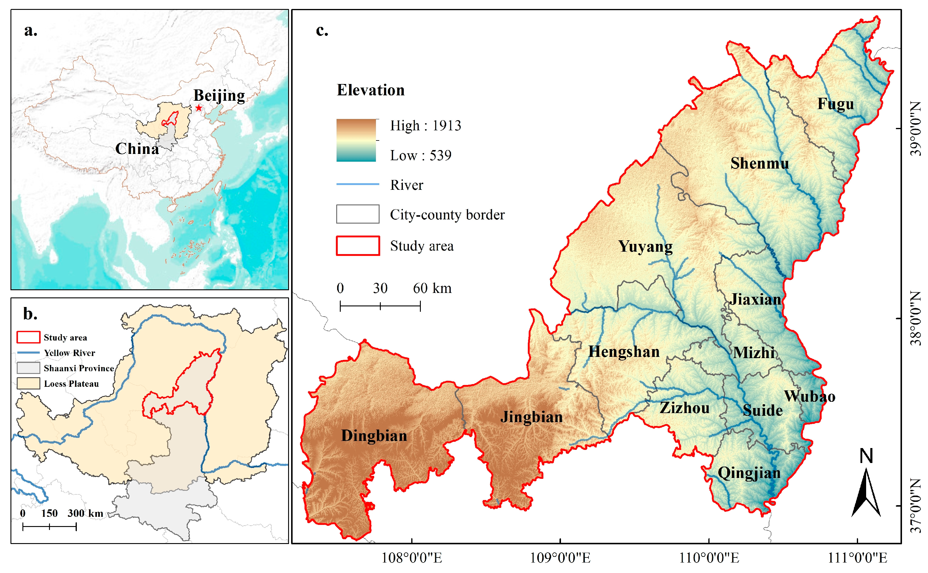
2.1. Study Area
2.2. Data Collection
2.3. Methods of CES Quantification
2.3.1. Quantifying the Supply and Demand of CESs
- (1)
- Quantifying CES supply
- (2)
- Quantifying CES demand
2.3.2. Identifying the Supply–Demand Matching of CES
2.3.3. Evaluating the Spatial Flow of CESs
3. Results
3.1. Supply and Demand Characteristics of CESs
3.1.1. Characteristics of CES Supply
3.1.2. Characteristics of CES Demand
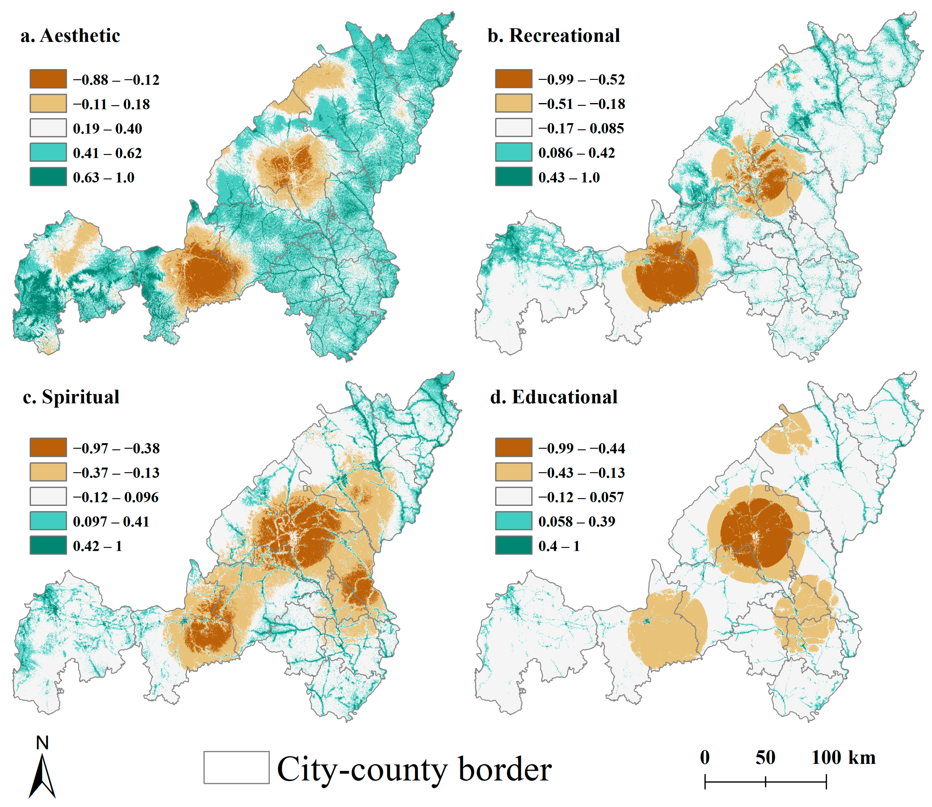
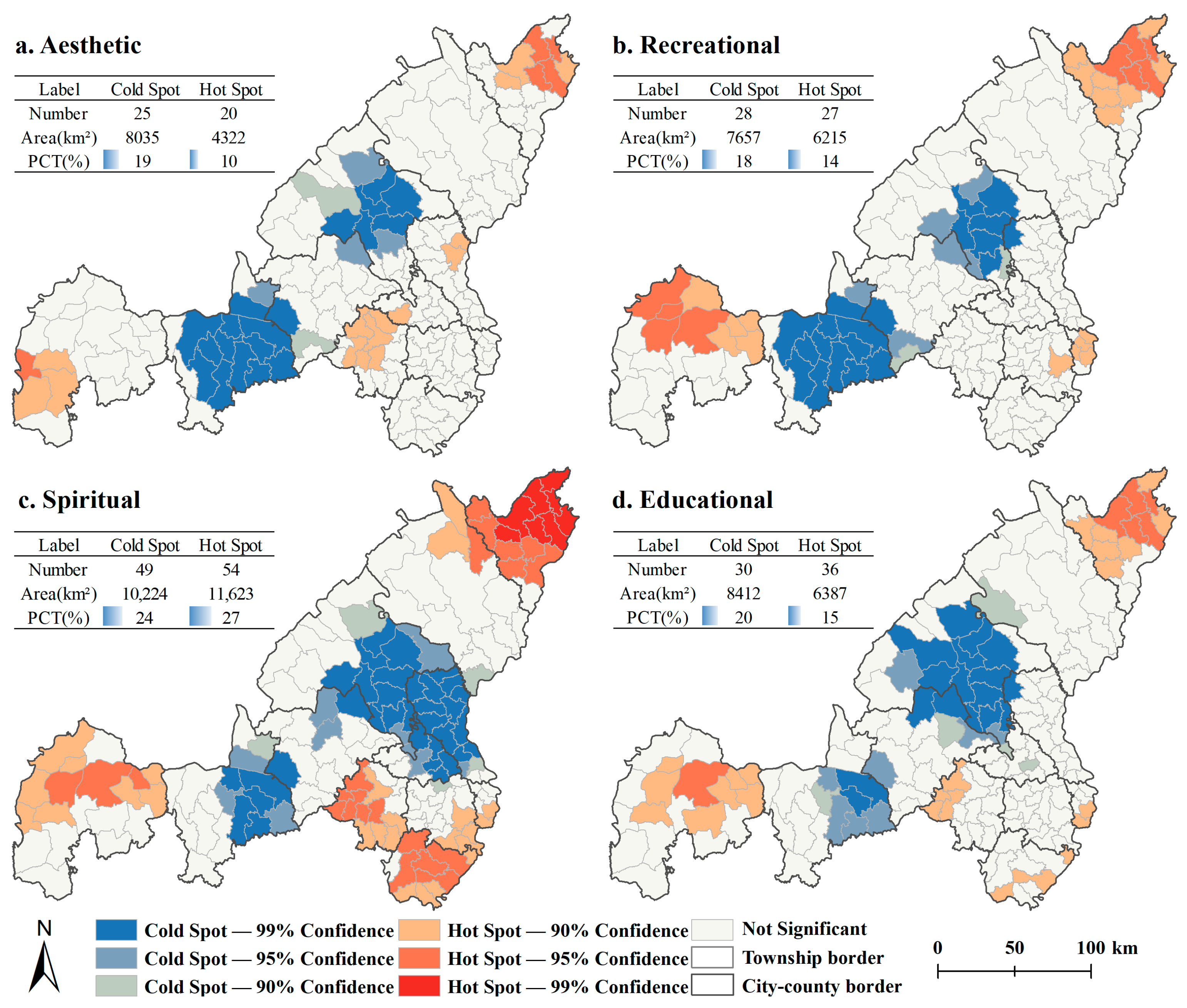
3.2. Mismatch of CES Supply–Demand
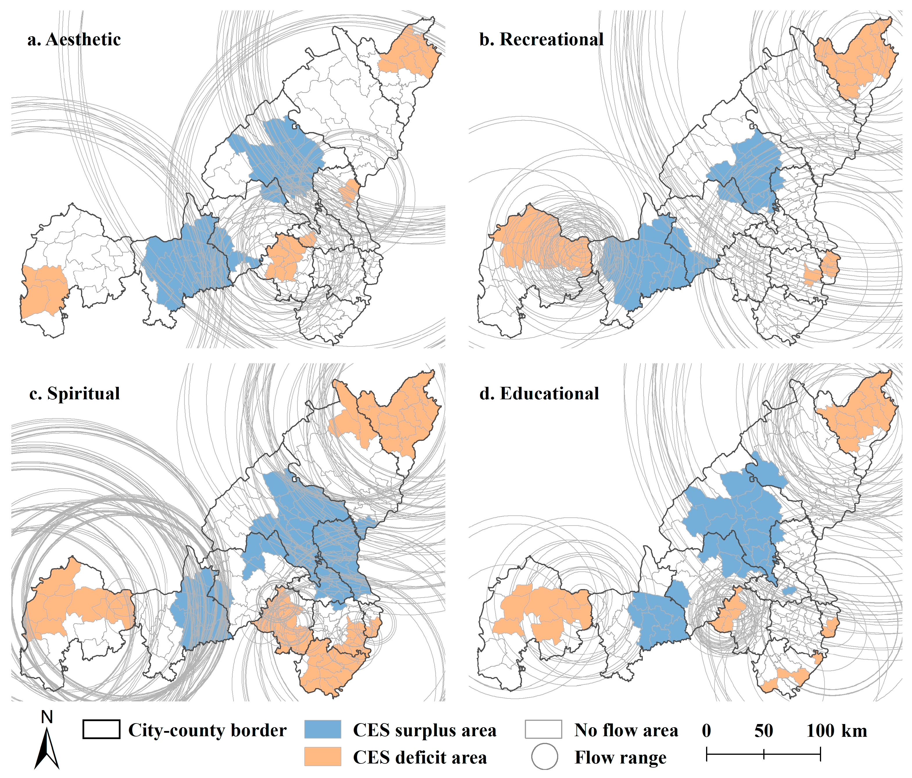
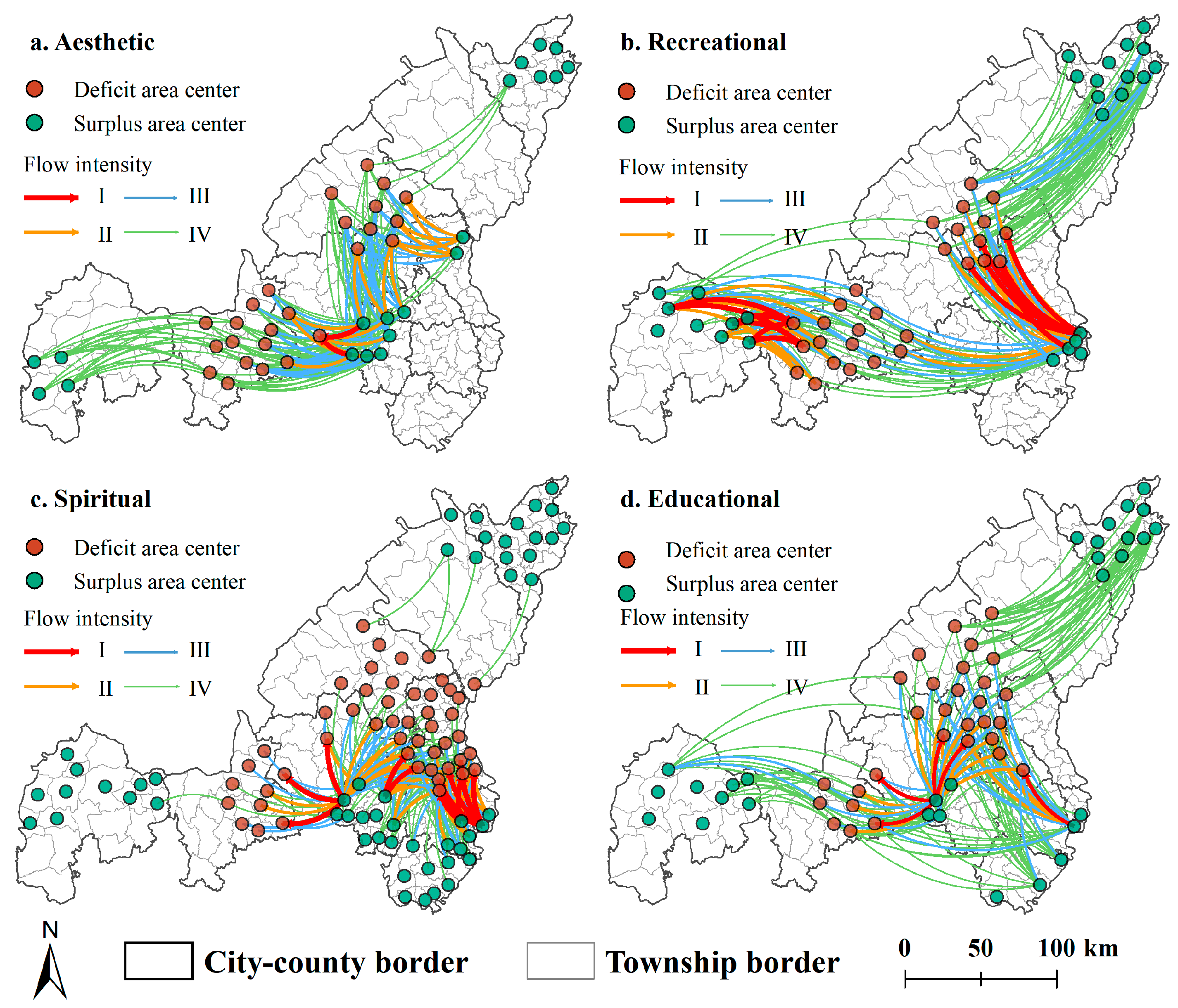
3.3. Spatial Flow Characteristics of CES
4. Discussion
4.1. CES Supply–Demand-Flow Characteristics
4.2. Recommendations for Urban Landscapes Management
4.2.1. Enhancing the Functionality of Low-Perception CESs
4.2.2. Alleviating the Supply–Demand Imbalance of CES
4.2.3. Optimizing the Spatial Flow of CESs
4.3. Limitations and Uncertainties
5. Conclusions
Author Contributions
Funding
Data Availability Statement
Conflicts of Interest
Appendix A


References
- MEA. Millennium Ecosystem Assessment: Ecosystems and Human Well-Being; Island Press: Washington, DC, USA, 2005. [Google Scholar]
- Kosanic, A.; Petzold, J. A systematic review of cultural ecosystem services and human wellbeing. Ecosyst. Serv. 2020, 45, 101168. [Google Scholar] [CrossRef]
- Daniel, T.C.; Muhar, A.; Arnberger, A.; Aznar, O.; Boyd, J.W.; Chan, K.M.A.; Costanza, R.; Elmqvist, T.; Flint, C.G.; Gobster, P.H.; et al. Contributions of cultural services to the ecosystem services agenda. Proc. Natl. Acad. Sci. USA 2012, 109, 8812–8819. [Google Scholar] [CrossRef]
- Margaryan, L.; Prince, S.; Ioannides, D.; Röslmaier, M. Dancing with cranes: A humanist perspective on cultural ecosystem services of wetlands. Tour. Geogr. 2018, 24, 501–522. [Google Scholar] [CrossRef]
- Wood, S.L.R.; Jones, S.K.; Johnson, J.A.; Brauman, K.A.; Chaplin-Kramer, R.; Fremier, A.; Girvetz, E.; Gordon, L.J.; Kappel, C.V.; Mandle, L.; et al. Distilling the role of ecosystem services in the Sustainable Development Goals. Ecosyst. Serv. 2018, 29, 70–82. [Google Scholar] [CrossRef]
- Pan, Y.; Qu, Y. Cultural Ecosystem Services in Land Use/Land Cover Change: A Literature Review and Prospects for Future Research. Land 2024, 13, 2027. [Google Scholar] [CrossRef]
- Zhao, Q.; Li, J.; Liu, J.; Cuan, Y.; Zhang, C. Integrating supply and demand in cultural ecosystem services assessment: A case study of Cuihua Mountain (China). Environ. Sci. Pollut. Res. Int. 2019, 26, 6065–6076. [Google Scholar] [CrossRef]
- Wang, L.; Zheng, H.; Wen, Z.; Liu, L.; Robinson, B.E.; Li, R.; Li, C.; Kong, L. Ecosystem service synergies/trade-offs informing the supply-demand match of ecosystem services: Framework and application. Ecosyst. Serv. 2019, 37, 100939. [Google Scholar] [CrossRef]
- Caputo, J.; Butler, B. Ecosystem service supply and capacity on U.S. family forestlands. Forests 2017, 8, 395. [Google Scholar] [CrossRef]
- Meng, S.T.; Huang, Q.X.; Zhang, L.; He, C.Y.; Inostroza, L.; Bai, Y.S.; Yin, D. Matches and mismatches between the supply of and demand for cultural ecosystem services in rapidly urbanizing watersheds: A case study in the Guanting Reservoir basin, China. Ecosyst. Serv. 2020, 45, 101156. [Google Scholar] [CrossRef]
- Jiang, W. Ecosystem services research in China: A critical review. Ecosyst. Serv. 2017, 26, 10–16. [Google Scholar] [CrossRef]
- Wei, H.; Liu, H.; Xu, Z.; Ren, J.; Lu, N.; Fan, W.; Zhang, P.; Dong, X. Linking ecosystem services supply, social demand and human well-being in a typical mountain–oasis–desert area, Xinjiang, China. Ecosyst. Serv. 2018, 31, 44–57. [Google Scholar] [CrossRef]
- Li, J.; Li, K.; Wang, Y.; Jiao, R. Comparative Study on the Perception of Cultural Ecosystem Services in Taibai Mountain National Forest Park from Different Stakeholder Perspectives. Land 2024, 13, 2207. [Google Scholar] [CrossRef]
- Lorilla, R.S.; Kalogirou, S.; Poirazidis, K.; Kefalas, G. Identifying spatial mismatches between the supply and demand of ecosystem services to achieve a sustainable management regime in the Ionian Islands (Western Greece). Land Use Pol. 2019, 88, 104171. [Google Scholar] [CrossRef]
- Lou, C.; Wang, F.; Li, G.; Yang, C. Identifying supply-demand spatial matches of cultural ecosystem services provided by urban parks in polycentric mountainous cities. Acta Ecol. Sin. 2024, 44, 5816–5827. [Google Scholar] [CrossRef]
- Hernández-Morcillo, M.; Plieninger, T.; Bieling, C. An empirical review of cultural ecosystem service indicators. Ecol. Indic. 2013, 29, 434–444. [Google Scholar] [CrossRef]
- Wartmann, F.M.; Purves, R.S. Investigating sense of place as a cultural ecosystem service in different landscapes through the lens of language. Landsc. Urban Plan. 2018, 175, 169–183. [Google Scholar] [CrossRef]
- Riechers, M.; Barkmann, J.; Tscharntke, T. Diverging perceptions by social groups on cultural ecosystem services provided by urban green. Landsc. Urban Plan. 2018, 175, 161–168. [Google Scholar] [CrossRef]
- Balázsi, Á.; Dänhardt, J.; Collins, S.; Schweiger, O.; Settele, J.; Hartel, T. Understanding cultural ecosystem services related to farmlands: Expert survey in Europe. Land Use Pol. 2021, 100, 104900. [Google Scholar] [CrossRef]
- Jeuring, J.H.G. Weather perceptions, holiday satisfaction and perceived attractiveness of domestic vacationing in The Netherlands. Tour. Manag. 2017, 61, 70–81. [Google Scholar] [CrossRef]
- Zhao, J.; Zhang, N.; Liu, Z.; Zhang, Q.; Shang, C. SWAT model applications: From hydrological processes to ecosystem services. Sci. Total Environ. 2024, 931, 172605. [Google Scholar] [CrossRef]
- Lin, Y.; Dong, Z.; Zhang, W.; Zhang, H. Estimating inter-regional payments for ecosystem services: Taking China’s Beijing-Tianjin-Hebei region as an example. Ecol. Econ. 2020, 168, 106514. [Google Scholar] [CrossRef]
- Johnson, G.W.; Bagstad, K.J.; Snapp, R.R.; Villa, F. Service Path Attribution Networks (SPANs). Int. J. Agric. Environ. 2012, 3, 54–71. [Google Scholar] [CrossRef]
- Ouyang, X.; Wang, Z.; Zhu, X. Construction of the Ecological Security Pattern of Urban Agglomeration under the Framework of Supply and Demand of Ecosystem Services Using Bayesian Network Machine Learning: Case Study of the Changsha–Zhuzhou–Xiangtan Urban Agglomeration, China. Sustainability 2019, 11, 6416. [Google Scholar] [CrossRef]
- Shi, T.; Gao, F. Utilizing Multi-Source Geospatial Big Data to Examine How Environmental Factors Attract Outdoor Jogging Activities. Remote Sens. 2024, 16, 3056. [Google Scholar] [CrossRef]
- Richards, D.R.; Tunçer, B. Using image recognition to automate assessment of cultural ecosystem services from social media photographs. Ecosyst. Serv. 2018, 31, 318–325. [Google Scholar] [CrossRef]
- Wang, L.; Huang, L.; Cao, W.; Zhai, J.; Fan, J. Assessing grassland cultural ecosystem services supply and demand for promoting the sustainable realization of grassland cultural values. Sci. Total Environ. 2024, 912, 169255. [Google Scholar] [CrossRef]
- Yoshimura, N.; Hiura, T. Demand and supply of cultural ecosystem services: Use of geotagged photos to map the aesthetic value of landscapes in Hokkaido. Ecosyst. Serv. 2017, 24, 68–78. [Google Scholar] [CrossRef]
- Sinclair, M.; Ghermandi, A.; Sheela, A.M. A crowdsourced valuation of recreational ecosystem services using social media data: An application to a tropical wetland in India. Sci. Total Environ. 2018, 642, 356–365. [Google Scholar] [CrossRef]
- Inácio, M.; Gomes, E.; Bogdzevič, K.; Kalinauskas, M.; Zhao, W.; Pereira, P. Mapping and assessing coastal recreation cultural ecosystem services supply, flow, and demand in Lithuania. J. Environ. Manag. 2022, 323, 116175. [Google Scholar] [CrossRef]
- Ghermandi, A.; Sinclair, M. Passive crowdsourcing of social media in environmental research: A systematic map. Glob. Environ. Change 2019, 55, 36–47. [Google Scholar] [CrossRef]
- Zhao, Y.; You, W.; Lin, X.; He, D. Assessing the supply and demand linkage of cultural ecosystem services in a typical county-level city with protected areas in China. Ecol. Indic. 2023, 147, 109992. [Google Scholar] [CrossRef]
- Zhang, J.; He, C.; Huang, Q.; Li, J.; Qi, T. Evaluating the supply and demand of cultural ecosystem services in the Tibetan Plateau of China. Landsc. Ecol. 2022, 37, 2131–2148. [Google Scholar] [CrossRef]
- Sherrouse, B.C.; Semmens, D.J.; Ancona, Z.H. Social Values for Ecosystem Services (SolVES): Open-source spatial modeling of cultural services. Environ. Modell. Softw. 2022, 148, 105259. [Google Scholar] [CrossRef]
- Shi, X.; Zhao, X.; Pu, J.; Gu, Z.; Zhao, Q.; Feng, Y.; Zhou, S. Creating a monetization-SolVES model to visualize the cultural ecosystem services for promoting landscape conservation. J. Nat. Conserv. 2024, 77, 126521. [Google Scholar] [CrossRef]
- Yu, D.; Xiang, B. Discovering topics and trends in the field of Artificial Intelligence: Using LDA topic modeling. Expert Syst. Appl. 2023, 225, 120114. [Google Scholar] [CrossRef]
- Sun, L.; Yin, Y. Discovering themes and trends in transportation research using topic modeling. Transp. Res. Part C Emerg. Technol. 2017, 77, 49–66. [Google Scholar] [CrossRef]
- Zhang, J.; He, C.; Huang, Q.; Li, L. Understanding ecosystem service flows through the metacoupling framework. Ecol. Indic. 2023, 151, 110303. [Google Scholar] [CrossRef]
- Du, H.; Zhao, L.; Zhang, P.; Li, J.; Yu, S. Ecological compensation in the Beijing-Tianjin-Hebei region based on ecosystem services flow. J. Environ. Manag. 2023, 331, 117230. [Google Scholar] [CrossRef]
- Yang, H.; Sun, L.; Zhou, M.; Li, F. Trade-off analyses of ecosystem services during the reconstruction of grain production space in Loess Plateau:A case of Yulin City. Arid Land Geogr. 2022, 45, 226–236. [Google Scholar] [CrossRef]
- National Forestry and Grassland Administration. Available online: https://www.forestry.gov.cn/c/www/dfdt/545006.jhtml (accessed on 10 December 2023).
- Li, Y.; Cheng, W.; Zuo, W.; Zhang, L. Agricultural Vulnerability to Drought in China’s Agro-pastoral Ecotone: A Case Study of Yulin City, Shaanxi Province. Chin. Geogr. Sci. 2023, 33, 934–945. [Google Scholar] [CrossRef]
- Shaanxi Provincial Cultural Heritage Administration. Available online: https://wwj.shaanxi.gov.cn/wbxx/bkydww/lswhmc/ (accessed on 10 December 2023).
- Pan, J.; Ma, Y.; Cai, S.; Chen, Y.; Chen, Y. Distribution patterns of lake-wetland cultural ecosystem services in highland. Environ. Dev. 2022, 44, 100754. [Google Scholar] [CrossRef]
- Hynes, S.; Ghermandi, A.; Norton, D.; Williams, H. Marine recreational ecosystem service value estimation: A meta-analysis with cultural considerations. Ecosyst. Serv. 2018, 31, 410–419. [Google Scholar] [CrossRef]
- Kalinauskas, M.; Bogdzevic, K.; Gomes, E.; Inacio, M.; Barcelo, D.; Zhao, W.; Pereira, P. Mapping and assessment of recreational cultural ecosystem services supply and demand in Vilnius (Lithuania). Sci. Total Environ. 2023, 855, 158590. [Google Scholar] [CrossRef]
- Khosravi Mashizi, A.; Sharafatmandrad, M.; Alizadeh, R. Exploring plant diversity and aesthetic service of mountain and plain landscapes in semiarid ecosystems. J. Nat. Conserv. 2024, 82, 126740. [Google Scholar] [CrossRef]
- TEEB. The Economics of Ecosystems and Biodiversity; The United Nations Environment Programme: Nairobi, Kenya, 2010. [Google Scholar]
- Web Services API Downloads. Available online: https://lbs.amap.com/api/webservice/download (accessed on 25 March 2025).
- Li, Y.; Zhang, D.; Wang, K.; Huang, L. Supply-demand relationships of cultural ecosystem services in rural areas: A case study of Huzhou City, Zhejiang Province. Acta Ecol. Sin. 2022, 42, 6888–6899. [Google Scholar] [CrossRef]
- Zhao, Z.; Xiao, N.; Shen, M.; Li, J. Comparison between optimized MaxEnt and random forest modeling in predicting potential distribution: A case study with Quasipaa boulengeri in China. Sci. Total Environ. 2022, 842, 156867. [Google Scholar] [CrossRef]
- Zhang, K.; Yao, L.; Meng, J.; Tao, J. Maxent modeling for predicting the potential geographical distribution of two peony species under climate change. Sci. Total Environ. 2018, 634, 1326–1334. [Google Scholar] [CrossRef]
- Ma, M.; Yuan, W.; Ge, Q.; Yuan, W.; Yang, L.; Li, H.; Li, M. Big data analysis of social development situation in regions along the Belt and Road. Prog. Geogr. 2019, 38, 1009–1020. [Google Scholar] [CrossRef]
- Zhang, B.; Wang, H. A new type of dual-scale neighborhood based on vectorization for cellular automata models. GISci. Remote Sens. 2021, 58, 386–404. [Google Scholar] [CrossRef]
- Li, Y.; Li, Z.; Wang, J.; Zeng, H. Analyses of driving factors on the spatial variations in regional eco-environmental quality using two types of species distribution models: A case study of Minjiang River Basin, China. Ecol. Indic. 2022, 139, 108980. [Google Scholar] [CrossRef]
- Phillips, S.J.; Anderson, R.P.; Schapire, R.E. Maximum entropy modeling of species geographic distributions. Ecol. Modell. 2006, 190, 231–259. [Google Scholar] [CrossRef]
- Fielding, A.H.; Bell, J.F. A review of methods for the assessment of prediction errors in conservation presence/absence models. Environ. Conserv. 2002, 24, 38–49. [Google Scholar] [CrossRef]
- Phillips, S.J.; Anderson, R.P.; Dudík, M.; Schapire, R.E.; Blair, M.E. Opening the black box: An open-source release of Maxent. Ecography 2017, 40, 887–893. [Google Scholar] [CrossRef]
- Kong, W.; Li, X.; Zou, H. Optimizing MaxEnt model in the prediction of species distribution. Chin. J. Appl. Ecol. 2019, 30, 2116–2128. [Google Scholar] [CrossRef]
- Porfirio, L.L.; Harris, R.M.B.; Lefroy, E.C.; Hugh, S.; Gould, S.F.; Lee, G.; Bindoff, N.L.; Mackey, B. Improving the Use of Species Distribution Models in Conservation Planning and Management under Climate Change. PLoS ONE 2014, 9, e113749. [Google Scholar] [CrossRef]
- Farkhod, A.; Abdusalomov, A.; Makhmudov, F.; Cho, Y.I. LDA-Based Topic Modeling Sentiment Analysis Using Topic/Document/Sentence (TDS) Model. Appl. Sci. 2021, 11, 11091. [Google Scholar] [CrossRef]
- Elsayed, A.; Rixon, S.; Zeuner, C.; Levison, J.; Binns, A.; Goel, P. Text mining-aided meta-research on nutrient dynamics in surface water and groundwater: Popular topics and perceived gaps. J. Hydrol. 2023, 626, 130338. [Google Scholar] [CrossRef]
- Li, J.; Jiang, H.; Bai, Y.; Alatalo, J.M.; Li, X.; Jiang, H.; Liu, G.; Xu, J. Indicators for spatial–temporal comparisons of ecosystem service status between regions: A case study of the Taihu River Basin, China. Ecol. Indic. 2016, 60, 1008–1016. [Google Scholar] [CrossRef]
- Pan, Z.; He, J.; Liu, D.; Wang, J.; Guo, X. Ecosystem health assessment based on ecological integrity and ecosystem services demand in the Middle Reaches of the Yangtze River Economic Belt, China. Sci. Total Environ. 2021, 774, 144837. [Google Scholar] [CrossRef]
- Liu, H.; Remme, R.P.; Hamel, P.; Nong, H.; Ren, H. Supply and demand assessment of urban recreation service and its implication for greenspace planning-A case study on Guangzhou. Landsc. Urban Plan. 2020, 203, 103898. [Google Scholar] [CrossRef]
- Tianlin, Z.; Dou, Z.; Chenchen, Z. How to optimize ecological compensation to alleviate environmental injustice in different cities in the Yellow River Basin? A case of integrating ecosystem service supply, demand and flow. Sustain. Cities Soc. 2021, 75, 103341. [Google Scholar] [CrossRef]
- Xin, G.; Juqin, S.; Weijun, H.; Xu, Z.; Zhichao, L.; Weifang, H.; Jingzhe, W.; Yingjie, R.; Xin, Z. Spatial-temporal analysis of ecosystem services value and research on ecological compensation in Taihu Lake Basin of Jiangsu Province in China from 2005 to 2018. J. Clean. Prod. 2021, 317, 128241. [Google Scholar] [CrossRef]
- Su, D.; Cao, Y.; Dong, X.; Wu, Q.; Fang, X.; Cao, Y. Evaluation of ecosystem services budget based on ecosystem services flow: A case study of Hangzhou Bay area. Appl. Geogr. 2023, 162, 103150. [Google Scholar] [CrossRef]
- Cortinovis, C.; Zulian, G.; Geneletti, D. Assessing Nature-Based Recreation to Support Urban Green Infrastructure Planning in Trento (Italy). Land 2018, 7, 112. [Google Scholar] [CrossRef]
- Li, K.; Hou, Y.; Andersen, P.S.; Xin, R.; Rong, Y.; Skov-Petersen, H. An ecological perspective for understanding regional integration based on ecosystem service budgets, bundles, and flows: A case study of the Jinan metropolitan area in China. J. Environ. Manag. 2022, 305, 114371. [Google Scholar] [CrossRef]
- Chen, J.; Xu, M.; Su, X.; Gao, J. Spatial transfer of regional ecosystem service in Nanjing City. Acta Ecol. Sin. 2014, 34, 5087–5095. [Google Scholar] [CrossRef]
- Ma, Y.; Chen, H.; Yang, M.; Aihemaiti, G.; Lu, W.; Zhao, R. Ecological compensation based on multiscale ecosystem carbon sequestration service flow. J. Environ. Manag. 2024, 372, 123396. [Google Scholar] [CrossRef]
- Chi, C.; Shen, J.; Gao, X.; Hu, P.; Yi, P. Horizontal ecological compensation standards based on ecosystem services flow. Ecol. Indic. 2024, 163, 112081. [Google Scholar] [CrossRef]
- Yu, Y.; Li, J.; Han, L.; Zhang, S. Research on ecological compensation based on the supply and demand of ecosystem services in the Qinling-Daba Mountains. Ecol. Indic. 2023, 154, 110687. [Google Scholar] [CrossRef]
- Wu, C.; Lu, R.; Zhang, P.; Dai, E. Multilevel ecological compensation policy design based on ecosystem service flow: A case study of carbon sequestration services in the Qinghai-Tibet Plateau. Sci. Total Environ. 2024, 921, 171093. [Google Scholar] [CrossRef]
- Pinto, L.V.; Inacio, M.; Bogdzevic, K.; Kalinauskas, M.; Gomes, E.; Pereira, P. Factors affecting cultural ecosystem services use in Vilnius (Lithuania): A participatory mapping survey approach. Heliyon 2023, 9, e15384. [Google Scholar] [CrossRef]
- Li, J.; Geneletti, D.; Wang, H. Understanding supply-demand mismatches in ecosystem services and interactive effects of drivers to support spatial planning in Tianjin metropolis, China. Sci. Total Environ. 2023, 895, 165067. [Google Scholar] [CrossRef]
- Dang, H.; Li, J. Supply-demand relationship and spatial flow of urban cultural ecosystem services: The case of Shenzhen, China. J. Clean. Prod. 2023, 423, 138765. [Google Scholar] [CrossRef]
- Zhao, Q.; Li, J.; Cuan, Y.; Zhou, Z. The Evolution Response of Ecosystem Cultural Services under Different Scenarios Based on System Dynamics. Remote Sens. 2020, 12, 418. [Google Scholar] [CrossRef]
- Wu, J.; Huang, Y.; Jiang, W. Spatial matching and value transfer assessment of ecosystem services supply and demand in urban agglomerations: A case study of the Guangdong-Hong Kong-Macao Greater Bay area in China. J. Clean. Prod. 2022, 375, 134081. [Google Scholar] [CrossRef]
- Clemente, P.; Calvache, M.; Antunes, P.; Santos, R.; Cerdeira, J.O.; Martins, M.J. Combining social media photographs and species distribution models to map cultural ecosystem services: The case of a Natural Park in Portugal. Ecol. Indic. 2019, 96, 59–68. [Google Scholar] [CrossRef]
- Su, B.R.; Liu, M.C. An ecosystem service trade-off management framework based on key ecosystem services. Ecol. Indic. 2023, 154, 110894. [Google Scholar] [CrossRef]
- Ament, J.M.; Moore, C.A.; Herbst, M.; Cumming, G.S. Cultural Ecosystem Services in Protected Areas: Understanding Bundles, Trade-Offs, and Synergies. Conserv. Lett. 2016, 10, 440–450. [Google Scholar] [CrossRef]
- Cheng, X.; Van Damme, S.; Li, L.; Uyttenhove, P. Cultural ecosystem services in an urban park: Understanding bundles, trade-offs, and synergies. Landsc. Ecol. 2022, 37, 1693–1705. [Google Scholar] [CrossRef]
- Yıldırım, G.; Akamca, G.Ö. The effect of outdoor learning activities on the development of preschool children. S. Afr. J. Educ. 2017, 37, 1–10. [Google Scholar] [CrossRef]
- Dang, H.; Li, J.; Zhou, Z. Revealing the supply-demand relationship of urban cultural ecosystem services: The combination of open-source spatial model and topic model. Appl. Geogr. 2024, 167, 103288. [Google Scholar] [CrossRef]
- Yin, D.; Huang, Q.; He, C.; Hua, X.; Liao, C.; Inostroza, L.; Zhang, L.; Bai, Y. The varying roles of ecosystem services in poverty alleviation among rural households in urbanizing watersheds. Landsc. Ecol. 2022, 37, 1673–1692. [Google Scholar] [CrossRef]
- Chen, J.; Jiang, B.; Bai, Y.; Xu, X.; Alatalo, J.M. Quantifying ecosystem services supply and demand shortfalls and mismatches for management optimisation. Sci. Total Environ. 2019, 650, 1426–1439. [Google Scholar] [CrossRef] [PubMed]
- Syrbe, R.-U.; Walz, U. Spatial indicators for the assessment of ecosystem services: Providing, benefiting and connecting areas and landscape metrics. Ecol. Indic. 2012, 21, 80–88. [Google Scholar] [CrossRef]
- Huai, S.Y.; Chen, F.; Liu, S.; Canters, F.; van de Voorde, T. Using social media photos and computer vision to assess cultural ecosystem services and landscape features in urban parks. Ecosyst. Serv. 2022, 57, 101475. [Google Scholar] [CrossRef]
- He, S.; Su, Y.; Shahtahmassebi, A.R.; Huang, L.; Zhou, M.; Gan, M.; Deng, J.; Zhao, G.; Wang, K. Assessing and mapping cultural ecosystem services supply, demand and flow of farmlands in the Hangzhou metropolitan area, China. Sci. Total Environ. 2019, 692, 756–768. [Google Scholar] [CrossRef]
- Wang, Y.; Hayashi, K. Methodological development of cultural ecosystem services evaluation using location data. J. Clean. Prod. 2023, 396, 136523. [Google Scholar] [CrossRef]
- Zhu, W.; Zhang, Z.; Zhang, H.; Tovuudorj, R. Integrating spatial patterns and driving factors of cultural ecosystem services into territorial spatial governance: A case study of the Horqin Sandy Land with multi-ethnic settlements. Habitat Int. 2024, 148, 103093. [Google Scholar] [CrossRef]
- van Zanten, B.T.; Van Berkel, D.B.; Meentemeyer, R.K.; Smith, J.W.; Tieskens, K.F.; Verburg, P.H. Continental-scale quantification of landscape values using social media data. Proc. Natl. Acad. Sci. USA 2016, 113, 12974–12979. [Google Scholar] [CrossRef]


| Data | Description | Units | Year | Source |
|---|---|---|---|---|
| Geospatial data | LU: land use | / | 2022 | https://zenodo.org/records/12779975 (accessed on 10 December 2024) |
| Slope: terrain slope | degree | 2022 | https://www.gscloud.cn/ (accessed on 10 December 2024) | |
| DEM: digital elevation model | m | 2022 | https://www.gscloud.cn/ (accessed on 10 December 2024) | |
| NDVI: normalized difference vegetation index | / | 2022 | http://www.nesdc.org.cn/ (accessed on 1 August 2024) | |
| DicW: distance from water | m | 2022 | https://www.openstreetmap.org (accessed on 20 October 2024) | |
| DisR: distance from road | m | 2022 | https://www.openstreetmap.org (accessed on 20 October 2024) | |
| DisT: distance from town | m | 2022 | https://lbs.amap.com/ (accessed on 1 December 2023) | |
| User interaction data | POI with CES functions, including ID, latitude, longitude, and tags | / | 2023 | https://lbs.amap.com/ (accessed on 1 December 2023) |
| Website consumer comments text, including ID, latitude, longitude, time, ratings, and reviews | / | 2023 | https://www.dianping.com/ (accessed on 1 December 2023) | |
| Per capita GDP data | Gross Domestic Product Per Capita | / | 2022 | https://tjj.yl.gov.cn/tjsj/tjgb/ (accessed on 25 March 2025) |
| Types | Meaning | Tags | Keywords |
|---|---|---|---|
| Aesthetic | Natural landscapes with ornamental value and aesthetic enjoyment exemplify the ecological service value derived from the harmonious coexistence between humans and nature. | Tourist attractions; Natural place name | Scenic spot, pavilion, forest, pine, bamboo, apricot, plum, cliff, peak, valley, attraction; mountain, water, river, stream, lake, sea, ocean, pond, pool, waterfalls, shoal beach, wetland |
| Recreational | The capacity for recreational activities within the natural ecosystem reflects the values and needs tied to folklore and cultural traditions. | Recreation place; Holiday and Nursing resort | Leisure, square, camp, base, garden, village, slide, street; vacations, estates, hot springs |
| Spiritual | A place with spiritual or religious significance reflects the profound cultural and historical importance to humanity. | Buddhist and Taoist temple; Church; Mosque | Confucian, Buddhist, and Taoist temples, filial piety, virtue, ancient, history, |
| Educational | Sites designated for natural science research and educational activities. | Memorial hall; Science/Culture and Education service | Memorials, culture, humanities, auditoriums, pavilions, palaces, gardens, science, education |
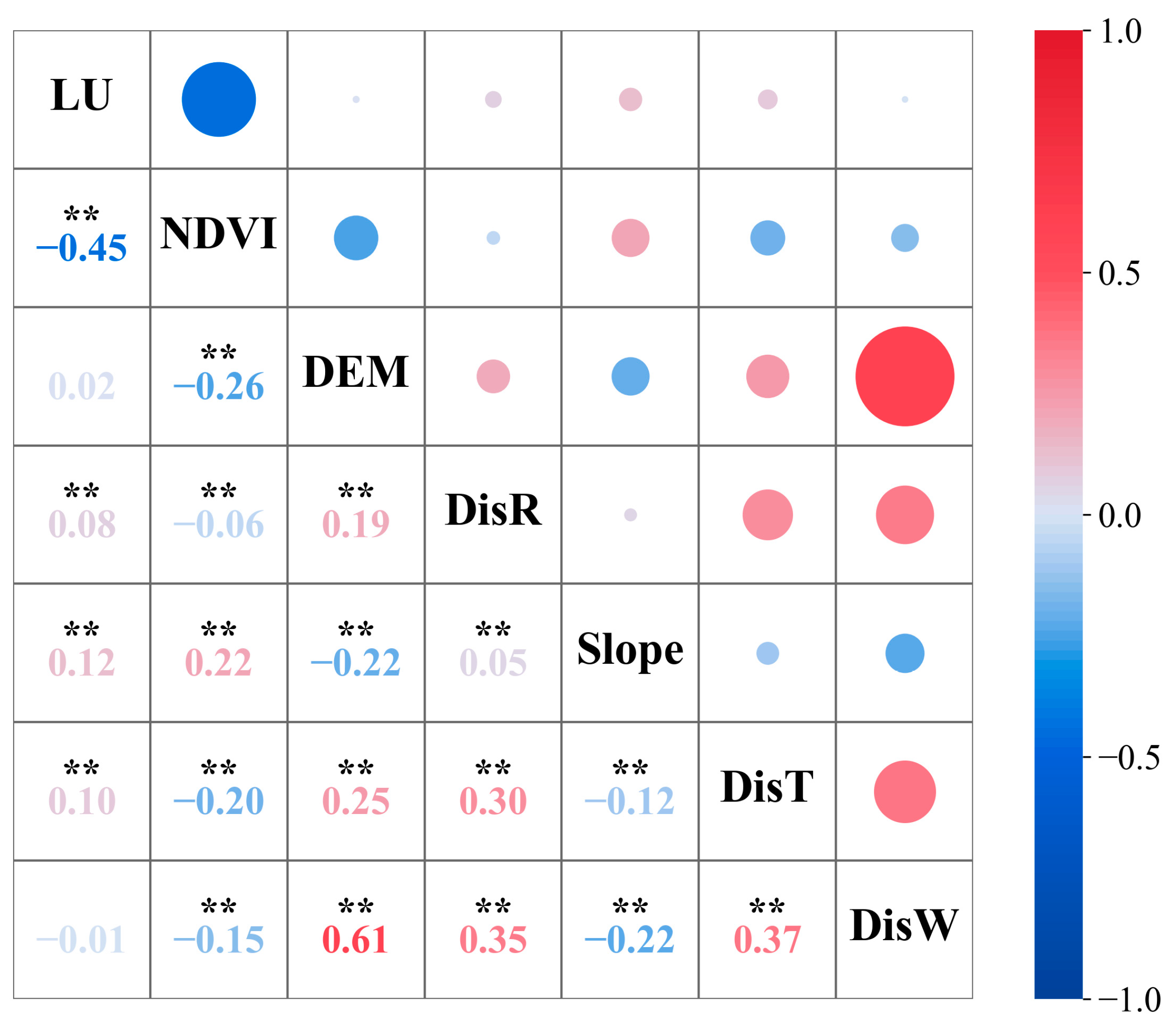
| CES | Environmental Factors | ||||||
|---|---|---|---|---|---|---|---|
| DisR | LU | DisW | NDVI | DEM | Slope | DisT | |
| Aesthetic | 7.8 | 17 | 38.3 | 3.8 | 23.9 | 6.8 | 2.3 |
| Recreation | 34 | 26.8 | 1.3 | 23.5 | 5.4 | 6.1 | 2.9 |
| Spiritual | 45.3 | 9.3 | 13.9 | 23.2 | 2.5 | 1.1 | 4.7 |
| Educational | 39.6 | 45.2 | 2 | 9.8 | 2 | 0.3 | 1.1 |
| Cumulative contribution | 126.7 | 98.3 | 55.5 | 60.3 | 33.8 | 14.3 | 11 |
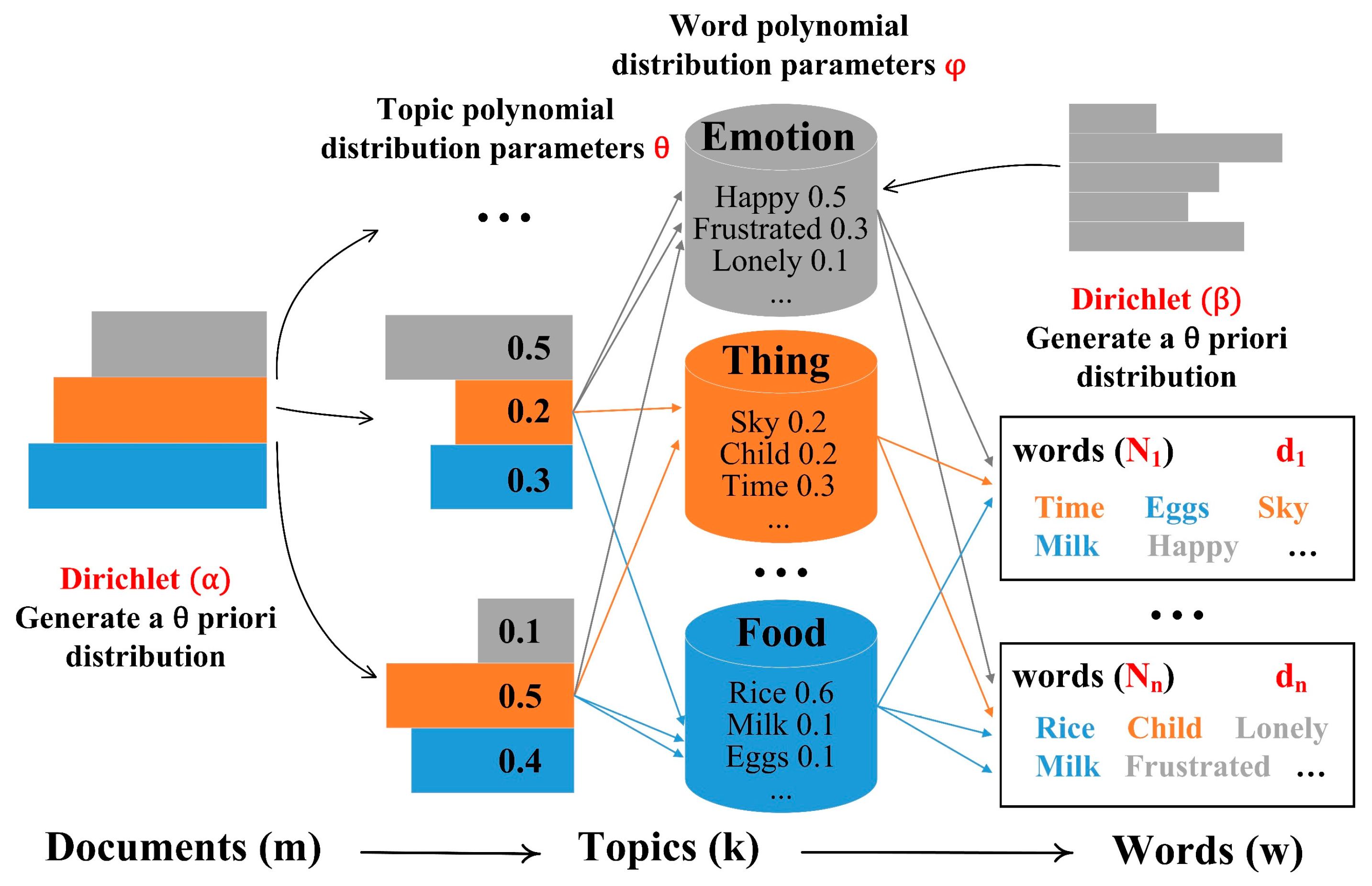
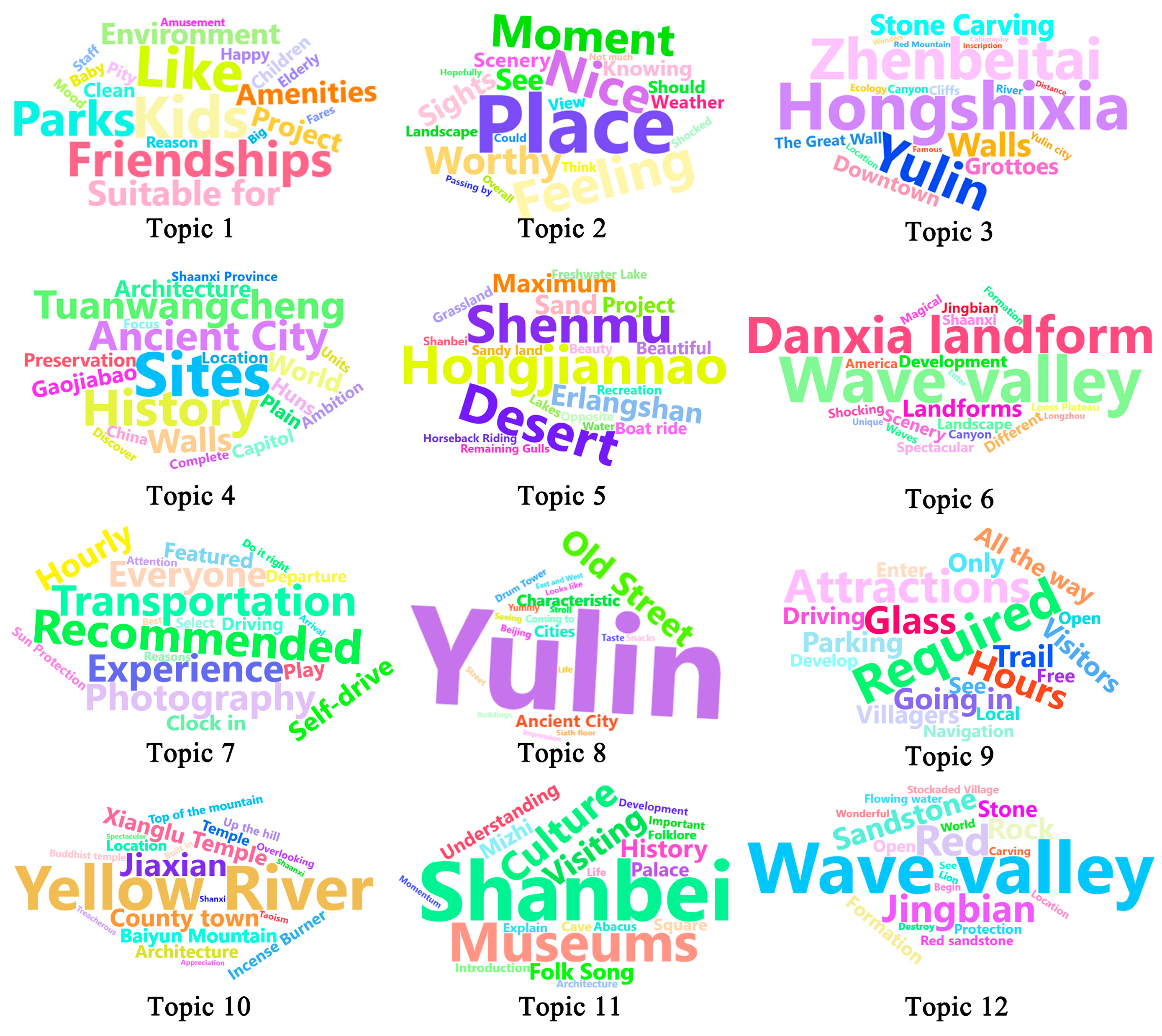
| CES Types | Topics | Words |
|---|---|---|
| Aesthetic | Topic3, Topic5, Topic6, Topic12 | Hongshixia, Zhenbeitai, Hongjiannao, Shenmu, Wave valley, Danxia landform, Red |
| Recreational | Topic2, Topic7, Topic8, Topic9 | Place, Feeling, Recommended, Transportation, Yulin, Old Street, Required, Attractions |
| Spiritual | Topic4, Topic10 | Sites, History, Ancient City, Yellow River, Jiaxian |
| Education | Topic1, Topic11 | Kids, Like, Friendships, Shanbei, Museums, Culture |
| Types | Transfer Count | Minimum Flow Radius (km) | Maximum Flow Radius (km) | Average Flow Intensity |
| Aesthetic | 500 | 12.80 | 162.85 | 5.15 |
| Recreational | 756 | 11.75 | 254.32 | 0.21 |
| Spiritual | 2646 | 11.26 | 211.20 | 1.43 |
| Educational | 900 | 10.87 | 223.53 | 0.29 |
Disclaimer/Publisher’s Note: The statements, opinions and data contained in all publications are solely those of the individual author(s) and contributor(s) and not of MDPI and/or the editor(s). MDPI and/or the editor(s) disclaim responsibility for any injury to people or property resulting from any ideas, methods, instructions or products referred to in the content. |
© 2025 by the authors. Licensee MDPI, Basel, Switzerland. This article is an open access article distributed under the terms and conditions of the Creative Commons Attribution (CC BY) license (https://creativecommons.org/licenses/by/4.0/).
Share and Cite
Li, L.; Bai, Y.; Yuan, X.; Li, F. Assessing the Supply–Demand Matching and Spatial Flow of Urban Cultural Ecosystem Services: Based on Geospatial Data and User Interaction Data. Land 2025, 14, 773. https://doi.org/10.3390/land14040773
Li L, Bai Y, Yuan X, Li F. Assessing the Supply–Demand Matching and Spatial Flow of Urban Cultural Ecosystem Services: Based on Geospatial Data and User Interaction Data. Land. 2025; 14(4):773. https://doi.org/10.3390/land14040773
Chicago/Turabian StyleLi, Linru, Yu Bai, Xuefeng Yuan, and Feiyan Li. 2025. "Assessing the Supply–Demand Matching and Spatial Flow of Urban Cultural Ecosystem Services: Based on Geospatial Data and User Interaction Data" Land 14, no. 4: 773. https://doi.org/10.3390/land14040773
APA StyleLi, L., Bai, Y., Yuan, X., & Li, F. (2025). Assessing the Supply–Demand Matching and Spatial Flow of Urban Cultural Ecosystem Services: Based on Geospatial Data and User Interaction Data. Land, 14(4), 773. https://doi.org/10.3390/land14040773