Article

Does Multidimensional Urban Morphology Affect Thermal Sensation? Evidence from Shanghai

College of Landscape Architecture, Nanjing Forestry University, Nanjing 210037, China
*
Author to whom correspondence should be addressed.
Land 2025, 14(4), 769; https://doi.org/10.3390/land14040769
Submission received: 15 March 2025 / Revised: 1 April 2025 / Accepted: 2 April 2025 / Published: 3 April 2025
(This article belongs to the Special Issue Potential for Nature-Based Solutions in Urban Green Infrastructure)

Abstract

:
The inappropriate thermal conditions resulting from increasingly severe climate issues have led to numerous complications for urban residents, decreased urban settlement comfort, and increased average and peak energy demands in built environments. Existing studies have demonstrated the significant influence of urban morphology (UM) on the urban thermal environment (UTE); however, at the meso-scale and macro-scale, UTE is often simplified to land surface temperature (LST) and building surface temperatures. To investigate the impact of UM on UTE, we developed an evaluation framework consisting of thermal sensing feedback (TSF) and LST. We employed the seven-level TSF scale to evaluate TSF data obtained from the Internet, emphasizing individualized thermal perceptions of urban spaces and reorienting UTE research towards a human-centric perspective. Using a regression model, we examined the relationships between two-dimensional and three-dimensional UM variables and UTE at the meso-scale in the central urban area of Shanghai, China, during August and December 2024. The results indicated the following: (1) The normalized difference vegetation index (NDVI), building density (BD), floor area ratio (FAR), impervious surface index (ISI), building height (BH), average building volume (ABV), sky view fraction (SVF), and building shape (BSsh) effectively explained TSF. However, area weighted mean shape index (SHAPEAM), aggregation index (AI), edge density (ED), elevation, building spacing (BSsp), and spatial congestion degree (SCD) showed no significant correlation with TSF. (2) Significant variables, including NDVI, FAR, ISI, UM, BD, and BH, exhibited opposite effects on cold perception in winter compared to heat perception in summer, indicating a consistent influence on thermal perception across seasons. (3) In summer, the significant variables SVF, BSsh, and ISI showed opposite effects on TSF and LST, while in winter, FAR demonstrated contrasting impacts on TSF and LST. The results of this study advance understanding of the mechanisms through which UM influences UTE, providing valuable insights for the development of sustainable, thermally comfortable urban environments.

1. Introduction

In 2024, the global average temperature has been approximately 1.55 °C above pre-industrial levels, marking the first year exceeding the 1.5 °C threshold established by the Paris Agreement. This severe climatic situation underscores the necessity for urban planners and designers to create more attractive, thermally comfortable, and sustainable urban environments. Amid intensified global urban expansion, alterations in urban surface properties and structural characteristics have significantly affected urban-scale energy balance and microclimatic conditions [1]. Consequently, this has intensified climate change phenomena, increased the frequency of extreme weather events [2], and exacerbated urban heat islands (UHIs) [3].
For urban residents, the urban thermal environment (UTE) is a critical indicator of urban life quality and well-being and significantly impacts urban activity. Adverse UTE often causes dermatological issues, cardiovascular strain, heart attacks, strokes, respiratory distress, psychological disorders, and increased mortality among vulnerable populations [4]. The human perception of thermal comfort, essentially determined by the equilibrium between body heat production and dissipation rates, generates subjective sensations of cold or heat. Thermal neutrality, characterized by balanced heat exchange, corresponds with comfort.
Historically, UTE characterization has been limited primarily to land surface temperature (LST) measurements or data obtained from fixed and mobile devices, providing straightforward but effective assessments at macroscales [5]. However, individual-level thermal comfort in urban settings cannot be accurately represented by simple temperature indices alone. The first thermal comfort evaluation index, effective temperature (ET), emerged in the 1920s [6]. Subsequent development has produced comprehensive frameworks emphasizing psychological, physiological, and energy dimensions [7] or physiological, psychological, and physical dimensions [8]. Physical parameters typically include air temperature, airflow velocity, solar radiation, and relative humidity. Physiological factors involve skin temperature, perspiration rate, clothing insulation, and activity levels. Psychological factors are particularly complex, encompassing social habits and behavioral patterns [9].
ASHRAE Standard 55 [10] defines thermal comfort as a subjective state of satisfaction with the thermal environment, involving both objective environmental parameters and subjective physiological factors such as health, endurance, and adaptability. Hence, comprehensive assessments combining subjective perceptions and objective data are typically necessary [11]. In 1970, P.O. Fanger introduced the influential Predicted Mean Vote (PMV) index, based on air temperature, radiant temperature, airflow velocity, humidity, and two human-body-related variables [12]. PMV is recognized by ISO 7730 [13] and ASHRAE Standard 55–92 [10], though it is predominantly applied within built environments [14]. Outdoor thermal perception, influenced by spatiotemporal human–climate interactions, encompasses diverse and dynamic thermal experiences and expectations [15], requiring approaches beyond static temperature regulation. Outdoor thermal comfort refers explicitly to an individual’s degree of satisfaction or discomfort within urban environments [4]. Common indicators for outdoor thermal comfort include Wet Bulb Globe Temperature (WBGT) [16,17], Universal Thermal Climate Index (UTCI) [17,18,19], and Physiologically Equivalent Temperature (PET) [20], widely employed in evaluating long-term climate impacts and microclimatic conditions. These indices vary temporally (instantaneous to long-term) and spatially (micro-, meso-, and macro-scale), necessitating climate-zone-specific calibration for practical application.
At the micro-scale, researchers often rely on physiological parameters, such as body temperature and heart rate variability (HRV)—correlated with metabolic rate, oxygen saturation, and blood pressure—to objectively assess individual thermal comfort [21,22,23,24]. However, physiological indicators alone do not entirely capture UTE perception; memory, adaptation, and expectation significantly influence comfort assessments [25,26], requiring further characterization through standardized scales [27]. Practically, PMV and Actual Mean Vote (AMV) discrepancies are common [28,29]. Studies suggest that populations tolerate higher temperatures in colder climates and prefer lower temperatures in hot climates [30,31]. Neutral thermal conditions (PMV = 0) are not universally optimal [32], prompting researchers to incorporate thermal preference scales alongside comfort judgments for accuracy [33]. Consequently, the concept of “semantic shift” can be interpreted as a dynamic “neutral point” on the ASHRAE thermal comfort scale, where the optimal thermal comfort value is not fixed at neutrality (zero). Analysis of the ASHRAE scale’s underlying dynamics suggests the need to consider not only individuals’ perceived thermal state (e.g., feeling warm or cool) but also their desired thermal state [32].
Concerned by the adverse evolution of urban temperatures, researchers utilize quantitative indicators to analyze urban morphology (UM) impacts on UTE from an urban planning perspective [3]. Techniques including regression models, Geodetector analysis, and machine learning (network regression, Random Forest, eXtreme Gradient Boosting, and Convolutional Neural Networks) [34] have clarified the complex relationships between UTE and various indicators. Influencing factors are traditionally categorized as follows: (1) spatial morphology, emphasizing landscape features affecting microclimate regulation and shading [35], urban density generating internal heat, and impermeable surfaces (concrete, asphalt) absorbing solar radiation; (2) climatic conditions [36]; and (3) socio-economic factors (GDP, population, nighttime illumination) [37].
The influence of UM indices on UTE varies across macro-, meso-, local-, and micro-scales. Different scales offer distinct yet interactive insights, ranging from macro-scale remote sensing-based LST measurements [38] to local-scale Local Climate Zones (LCZs) classifications by Stewart and Oke [3,39,40,41], and micro-scale physiological and individual feedback evaluations. Such scale-specific research effectively elucidates urban microclimatic dynamics and their implications for human thermal comfort.
At present, Pearson, Spearman, and other relevant correlation models have been employed to investigate the impact of UM on TSF. However, these models typically neglect the synergistic relationships among various urban morphology variables, resulting in insufficient integration between micro-scale and macro-, meso-, and local-scale analyses. Previous studies have demonstrated the feasibility of utilizing Internet-based big data to establish multi-scale correlations linking individual perceptions, such as noise perception, with urban morphology [42]; however, equivalent research specifically addressing TSF remains unexplored. To address this research gap, this study examines the influence of UM on the UTE in the central urban area of Shanghai by comprehensively analyzing both two-dimensional land use and three-dimensional architectural forms, emphasizing correlations with TSF. Specifically, the study addresses three key questions: (1) How do UM variables independently and jointly influence LST and TSF? (2) What mechanisms account for the differential impacts of UM variables on TSF and LST? (3) How can UM shaping effectively regulate UTE at both LST and TSF levels?

2. Study Area and Data Sources
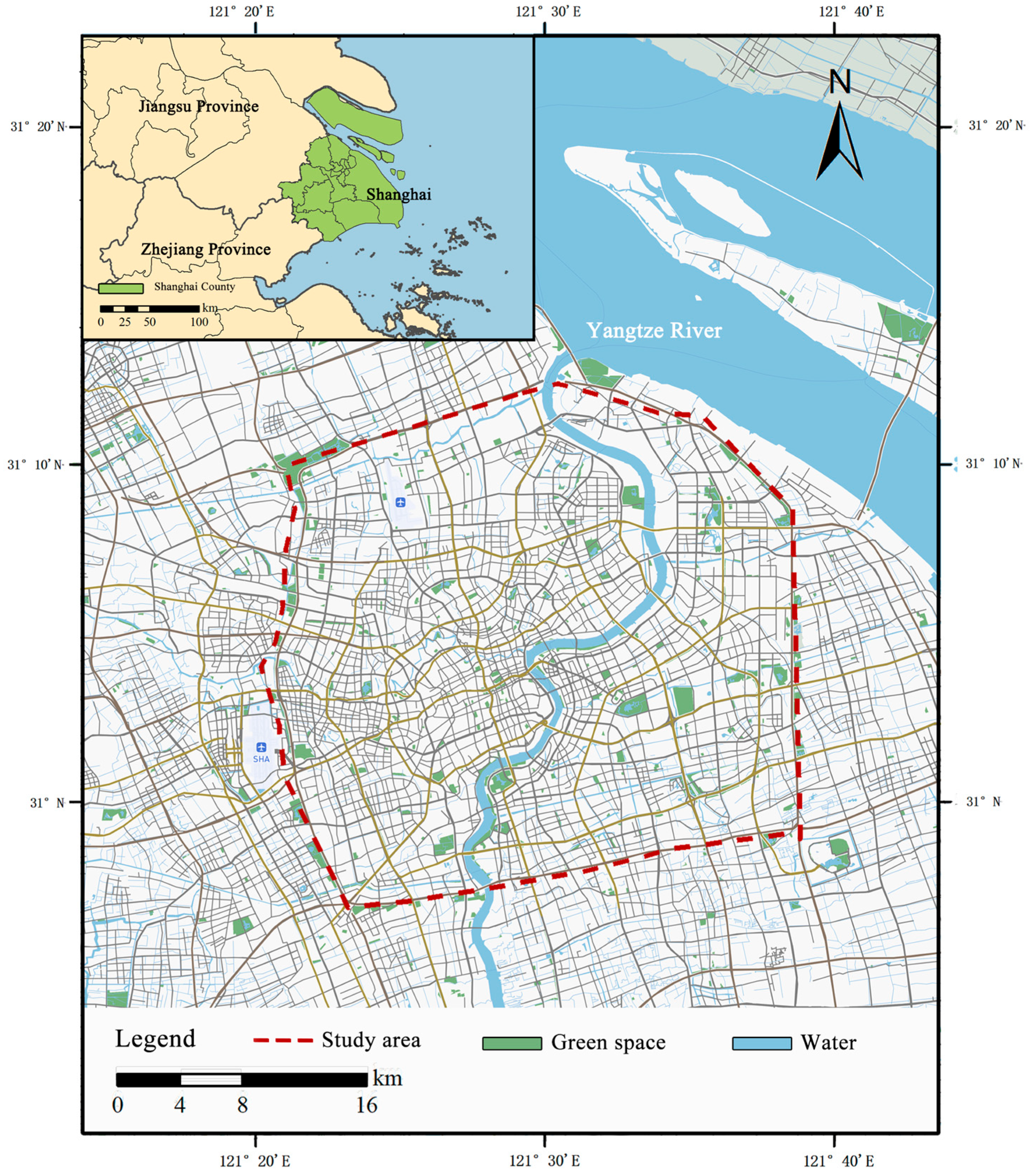
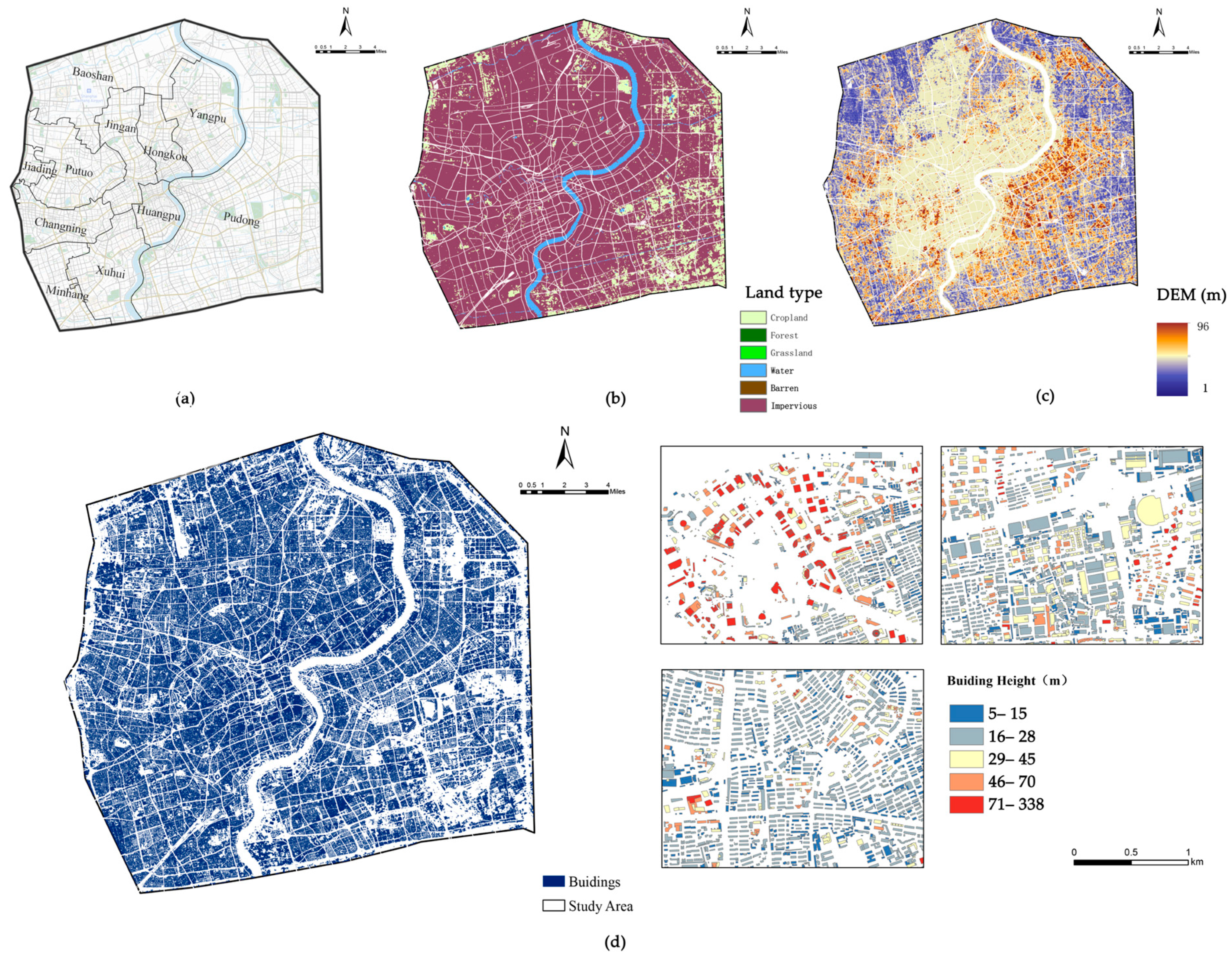
2.1. Study Area

The study was conducted in the central urban area of Shanghai, China (see Figure 1). Shanghai is located in the alluvial plain of the Yangtze River Delta, with a flat topography and subtropical monsoon climate. The average annual temperature is 17.7 °C, and the average yearly precipitation is 1086.8 mm. The central urban area of Shanghai is delineated as the region within the Shanghai Outer Ring Expressway, with an area of about 664 square kilometers and a planned resident population of about 11 million. The surface spatial pattern dataset of the study area is comprehensive and openly accessible; the residential and living population is dense, the young and middle-aged groups are active, and the Internet socializing activities are rich and varied.
To facilitate this study, the research area was divided into grid cells. Typically, grid resolutions ranging from 100 to 500 m are selected for urban form research [43]. Aggregation units at varying scales yield different insights into spatial characteristics [44], and differing grid scales influence experimental outcomes [45]. A grid resolution of 300 m × 300 m was selected, as it satisfies the requirements for statistical analysis of spatial form indicators while accurately capturing surface temperature inversion results. Grid units were generated using the fishnet tool in ArcGIS 10.8.1, and all spatial data utilized in this study were reprojected to match the spatial reference system of the grid.

2.2. Data Resources

2.2.1. Acquisition and Calibration of Remote Sensing Images of Urban Surface Space

Landsat-8 imagery (Band 10, originally at 100 m spatial resolution and resampled to 30 m) was collected to retrieve LST using the radiative transfer equation method [46]. Remote sensing allows detailed observation of surface characteristics, providing significant advantages for surface thermal environment studies [47]. High-precision infrared remote sensing data further enable detailed measurements of urban surface temperatures [2].
In China, spring typically spans from March to May, summer from June to August, autumn from September to November, and winter from December to February. This study specifically addresses thermal conditions in the hot summer and the cold winter. In 2024, Shanghai experienced significant warming, recording 52 high-temperature days (≥35 °C)—the second-highest in historical records—with 23 days reaching extreme heat levels (≥37 °C). Notably, a 12-day heatwave occurred between July 31 and August 11, breaking the 152-year record for consecutive high-temperature days. These climatic events are closely linked to global warming trends. In the winter of 2024, the central urban area of Shanghai faced notable cold extremes. Specifically, the maximum temperature on February 23–24 was just 2.2 °C, marking the coldest period recorded in late February over the past 43 years. All available images from January 1 to February 29, June 1 to August 31, and December 1 to 31, 2024, were screened, with only imagery from August 11 and December 17 meeting cloud-free conditions in the study area. The weather on these selected dates and preceding days was characterized by calm winds and no rainfall (https://rp5.ru (accessed on 25 February 2025)), resulting in high-quality data. Multi-spectral bands used in the study had a spatial resolution of 30 m. Image preprocessing included geometric corrections, radiometric calibration, atmospheric correction, and cropping.

2.2.2. Acquisition and Management of Urban Surface Spatial Morphology Data in Central Urban Area of Shanghai

The building vector data required for the calculation of urban surface spatial morphology indicators in the central area of Shanghai were obtained from the Resource and Environmental Science Data Platform (https://www.resdc.cn/ (accessed on 28 February 2025)) of the Institute of Geographic Sciences and Resources of the Chinese Academy of Sciences (IGSR). The Digital Elevation Model (DEM) data of the central urban area of Shanghai were obtained from the Geospatial Data Cloud (http://www.gscloud.cn/ (accessed on 28 February 2025)) (see Figure 2).

2.2.3. Acquisition of TSF Social Media Data

Social media data provide valuable insights into human activities and emotional states within urban areas, enabling researchers to investigate potential directions in urban planning, management, and development [48]. Comments on social media platforms are typically unstructured; hence, converting these data into analyzable information requires advanced text mining and analysis techniques [49]. Since 2009, China has introduced various social media platforms such as Sina Weibo and Dianping, where users can share text, images, and other information. Using GPS-enabled smart devices, users can also share their real-time geographic locations. The act of publicly sharing one’s environment, physical sensations, and emotional states on social media is referred to as “checking in”. Location-Based Social Network Services (LBSNS) have progressively become significant channels through which individuals share daily experiences and express real-time emotions. According to the Weibo User Consumption Trend Report published in December 2024, Weibo has reached 587 million monthly active users and 257 million daily active users.
In selecting the research period, priority was given to continuous intervals exhibiting distinctly cold or hot climates accompanied by favorable weather conditions. Consequently, August and December 2024 were selected as representative intervals for summer and winter analysis, respectively. Remote sensing data collected for this study were also derived from these two periods. Geo-tagged, weather-related comments posted on Sina Weibo during these periods were collected, specifically filtering for texts containing explicit descriptions of perceived heat or cold (e.g., “The sun is melting me today” or “The wind is biting”). User-generated spatiotemporal data were compiled into an Excel database and subsequently integrated with geographic location data using ArcGIS 10.8.1, establishing a foundational geospatial database for further analysis.

3. Methodology

3.1. Selection and Treatment of UM Indicators

As multi-layered and highly interactive systems, urban morphology is closely related to two-dimensional landscape patterns and three-dimensional building patterns [42,50]. We selected 14 UM variables related to TSF and LST, including 8 two-dimensional variables and 6 three-dimensional variables. Two-dimensional variables include normalized difference vegetation index (NDVI), building density (BD), floor area ratio (FAR), building spacing (BSsp), impervious surface index (ISI), area weighted mean shape index (SHAPEAM), aggregation index (AI), and edge density (ED). The three-dimensional variables include elevation, building height (BH) and average building volume (ABV), sky view fraction (SVF), building shape (BSsh), and spatial congestion degree (SCD) (see Table 1).

3.2. LST Retrieval

LST retrieval was conducted using Landsat-8 imagery, obtained from the Thermal Infrared Sensor (TIRS) onboard the Landsat-8 satellite and accessed via the United States Geological Survey (https://www.usgs.gov/landsat-missions/landsat-8 (accessed on 25 February 2025)). The primary thermal infrared bands employed for surface temperature retrieval are bands 10 and 11, with band 10 exhibiting higher atmospheric transmittance, making it particularly suitable for accurate surface temperature inversion.
Surface temperature was derived using the radiative transfer equation (RTE), where thermal infrared energy measured by satellite sensors is corrected for atmospheric effects. The formula is presented below:
L S T = K 2 ln K 1 B L S T + 1 273.15
P v = N D V I N D V I s o i l N D V I v e g N D V I s o i l
ε = 0.004 P v + 0.986
L λ = ε B L S T + ( 1 ε ) L d o w n τ + L u p
B L S T = L λ L u p τ ( 1 ε ) L d o w n τ ε
where P v represents the vegetation coverage fraction. N D V I v e g = 0.70 denotes the vegetation coverage in vegetated areas, while N D V I s o i l = 0.05 corresponds to the vegetation coverage in bare soil regions. ε is the surface emissivity. P v   refers to the overall vegetation coverage fraction within a mixed pixel. L λ stands for the infrared radiation heat value. B L S T represents the combined radiation brightness. τ is the atmospheric transmittance in the thermal infrared band. L u p and L d o w n are the upward and downward atmospheric radiation brightness, respectively. We use the NASA EARTHDATA (https://earthdata.nasa.gov/ (accessed on 25 February 2025)) for atmospheric parameters. K 1 and K 2 are constants, with K 1 = 774.8853   W m 2 s r 1 μ m 1 and K 2 = 1321.0789 K .

3.3. TSF Data Processing, Induction, and Quantification

As previously mentioned, due to the complex interplay of physical, physiological, and psychological factors influencing cold and heat perception, no single factor can comprehensively explain human thermal sensations. To simplify the experimental procedure and enhance feasibility, this study referenced the Thermal Sensation Vote (TSV) scale proposed by the American Society of Heating, Refrigerating, and Air-Conditioning Engineers (ASHRAE) and developed a 7-level Thermal Sensation Factor (TSF) scale (see Table 2). This scale is based on the laboratory-derived Predicted Mean Vote (PMV) model formulated by P.O. Fanger, who established correlations between thermal sensation and thermal balance through extensive laboratory observations [57]. By employing this scale, researchers can effectively capture spatial users’ immediate thermal sensations related to UTE. However, it should be noted that the TSF scale reflects immediate spatial experiences and does not comprehensively represent long-term thermal adaptability.
We preprocessed a total of 234,248 social media comment datasets to exclude advertisements, duplicate content, comments related to indoor environments, comments unrelated to TSF, and comments regarding specific outdoor spaces such as Shanghai Ice World. Ultimately, 3867 comments involving temperature perception feedback were selected, comprising 2276 in summer and 1591 in winter. A team of seven expert raters was assembled, and the seven-level TSF scale was employed to score the review text data item by item. Based on Fleiss’s Kappa test for inter-rater consistency, the differences among the seven groups of data were found to correlate with grade distance, and Linear Weights were applied to calculate Kappa values of 0.663 (>0.6), indicating moderate agreement and fulfilling the coefficient requirements for subjective tasks in social science research [58]. Additionally, p < 0.05 confirmed that the consistency was statistically significant. The final score was determined as the rounded average of the experts’ scores. The Thermal Feedback Orientation Index (TFOI) can be computed by integrating the degree of individual cold and hot perception with the frequency of each degree within the unit:
T F O I = ( S i F i )
where the sentiment temperature score ( S i ) for each comment is categorized and F i denotes the frequency of occurrence for each scale i , with i 3 , 2 , 1 , 0 , 1 , 2 , 3 .     T F O I stands for the overall intensity of thermal perception feedback within the unit, where a more positive value indicates a warmer perception, while a more negative value signifies a colder perception.

3.4. Model Selection

To assess how various variables influence the UTE, a regression analysis is required [59]. Common methods include Ordinary Least Squares (OLS) regression [36,60] and Geographically Weighted Regression (GWR) [61]. The traditional OLS regression model, widely employed in urban planning research [62], particularly for identifying relationships between urban thermal environments and their influencing factors [42], is considered the standard global regression approach [63]. Conversely, the GWR model is a local regression technique that requires data to exhibit spatial autocorrelation and demands a more rigorous sample size compared to OLS.
Spatial autocorrelation analysis was performed to characterize the spatial relationships and attribute similarities between each observation and adjacent statistical entities [64]. To assess spatial clustering, the Global Moran’s I statistic was computed individually for each variable through ArcGIS 10.8.1. The formula used in the calculations is as follows:
I = n i = 1 n j = 1 n w i j x i x ¯ ( x j x ¯ ) i = 1 n j = 1 n w i j i = 1 n x i x ¯ 2
where n is the total number of spatial units in the study area; x i and x j are the attribute values of the i and j th spatial units, respectively. x ¯ is the average of all spatial unit attribute values; w i j is the element in the spatial weight matrix that represents the spatial relationship between unit i and unit j . Values range from −1 to 1, where a positive value indicates a positive correlation, a negative value indicates a negative correlation, and a zero value indicates that there is no spatial autocorrelation [63]. In addition, the z-score needs to be calculated to determine whether the statistic significantly deviates from the expectation of the null hypothesis [61]. The calculation formula is as follows:
Z = I E I v a r I
If |Z| > 1.96, the null hypothesis is rejected, which indicates that Moran’s I is statistically significant at the 0.05 level.
After calculation, except AI, the Moran’s I values of UM variable data are all greater than 0.3, and |Z| > 1.96, indicating that there is a significant positive spatial correlation and a spatial clustering pattern. AI’s Moran’s I = 0.15, z = 22.7, and p = 0.000, indicating that there is a significant weak positive spatial autocorrelation in the data, that is, a non-random low-intensity clustering pattern in space. The Moran I values of the dependent variables TFOI in this study are all close to 0, and |Z| < 1.96, indicating that the distribution is random in space and there is no obvious global spatial autocorrelation. Therefore, OLS should be used as the research model in this study.
This study adopts the OLS model and takes it as the basic model of the research. OLS is expressed as follows:
Y = β 0 + β 1 X 1 + β 2 X 2 + + β n X n + ξ
where Y is the dependent variable; X 1 , X 2 X n is the explanatory variable; β is the estimated coefficient; and ξ is the random error.

4. Results

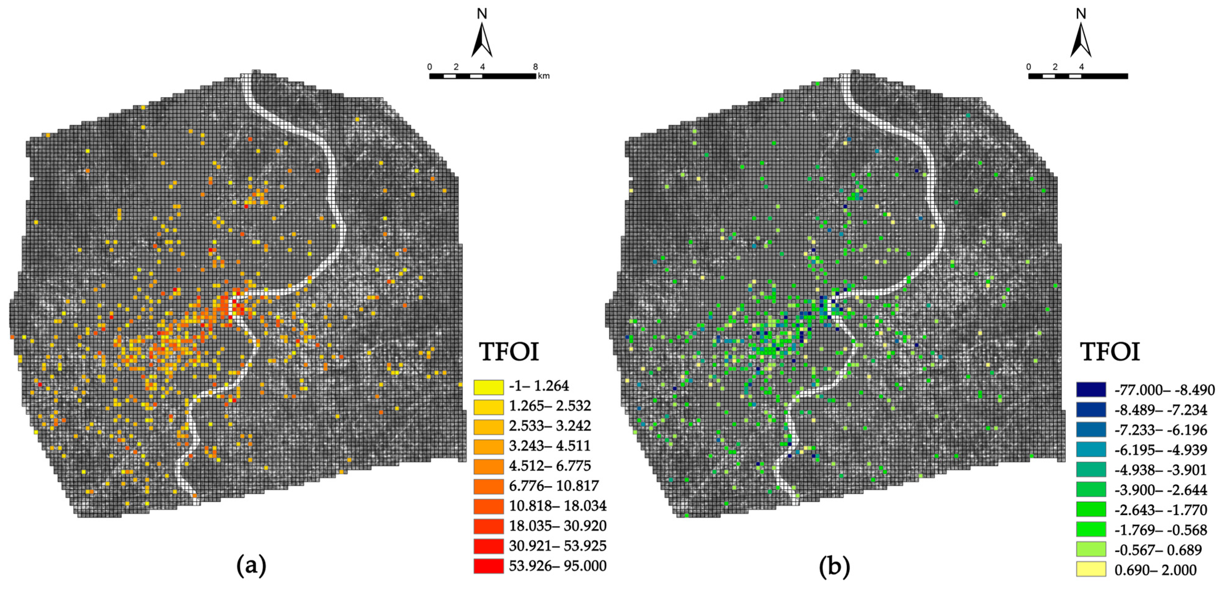
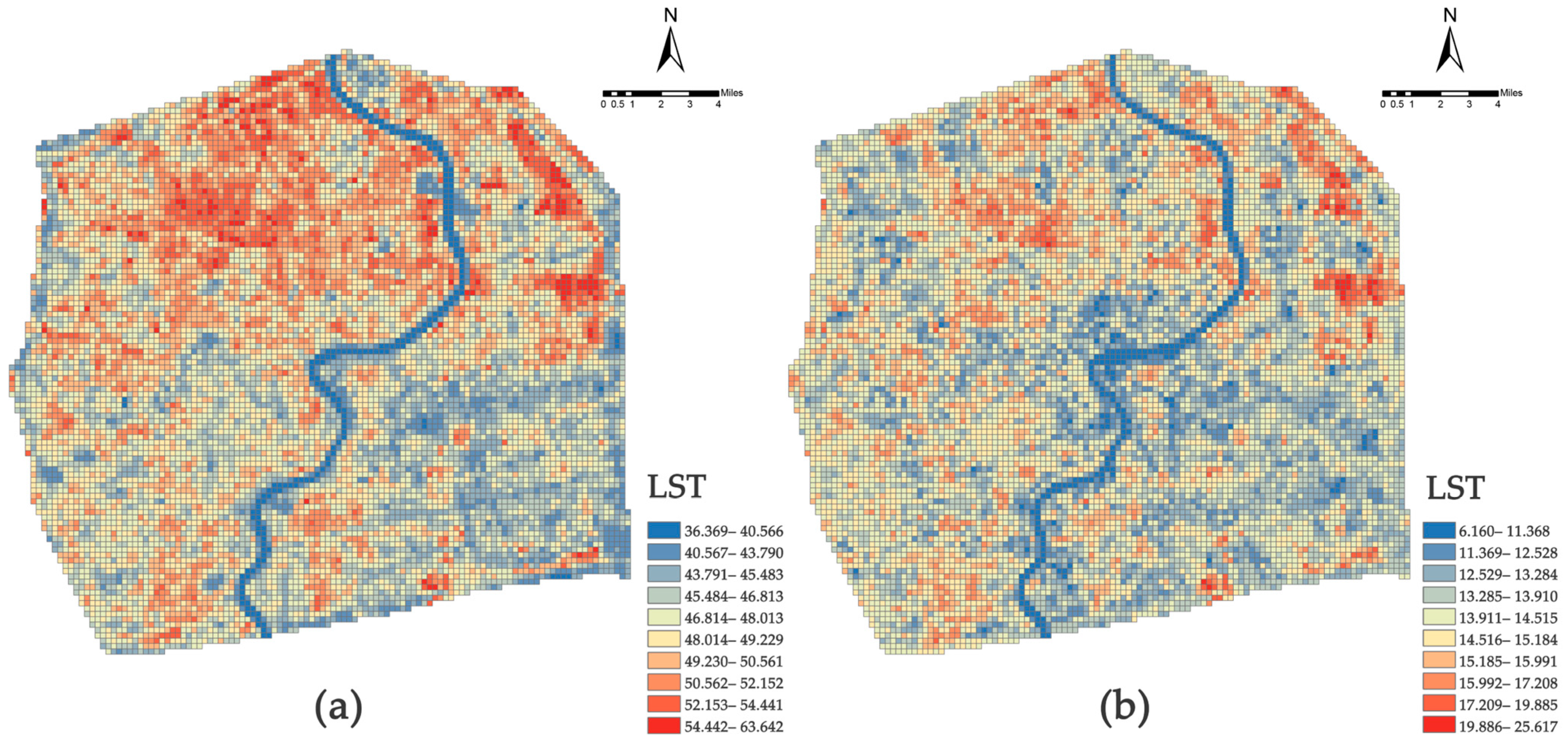
4.1. Spatial Distribution Characteristics of TSF and LST in the Central Urban Area of Shanghai

The calculated TFOI data were integrated with the geographical location data of comments and visualized in ArcGIS 10.8.1 to generate the TSF index map based on microblog sign-in data (as shown in Figure 3).
The calculated LST data were imported into ArcGIS 10.8.1 to generate the surface temperature map of the central urban area of Shanghai. As depicted in Figure 4, summer temperatures in the central urban area of Shanghai are generally elevated, with high-temperature zones predominantly concentrated in the Baoshan District, Yangpu District, Hongkou District, Jing’an District, and Pudong New Area, indicating pronounced urban heat island effects. The spatial distribution of temperature in winter exhibits a pattern similar to that observed in summer.

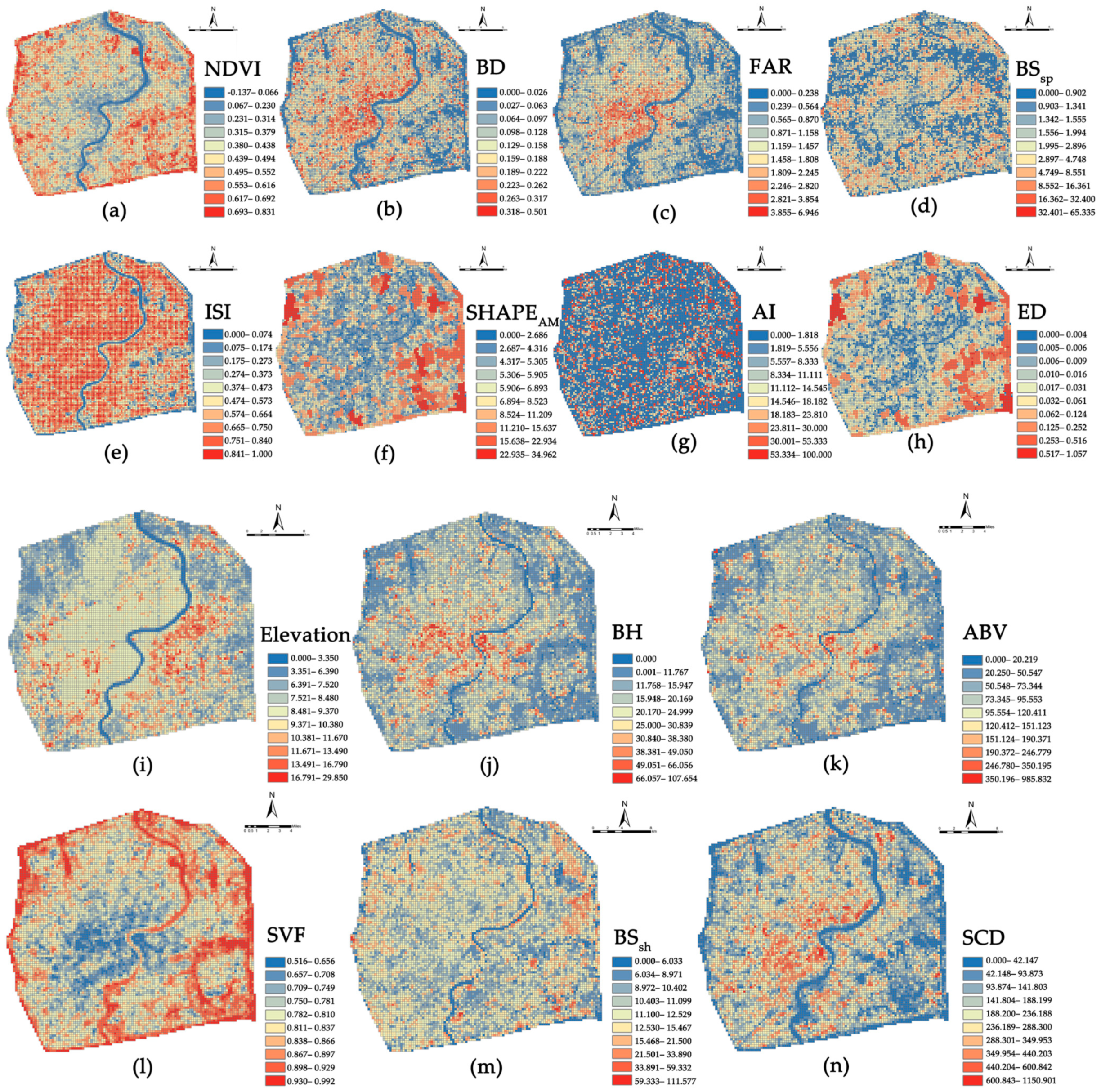
4.2. The Surface Spatial Form of the Central Urban Area of Shanghai

The spatial data for the central urban area of Shanghai were imported into ArcGIS 10.8.1 to calculate the UM index. As illustrated in Figure 5, UM in the central urban area of Shanghai exhibits complexity. The built environment in Huangpu District, Jing’an District, and Putuo District is characterized by high density and congestion. Urbanization diminishes gradually in a radial pattern from the central urban core outward. The peripheral wedge-shaped green belts demonstrate a higher rate of natural coverage. Additionally, the overall development intensity of the Pudong New Area is comparatively lower than that of the area north of the Huangpu River.
Considering that multicollinearity can lead to bias in the introduced OLS model and increase the standard error [65], we diagnosed the covariance in the linear regression of the UM data with the help of SPSS 26 before proceeding with the regression analysis of the OLS model. The VIF of all UM variables was tested to be less than 10. Therefore, all 14 indicators were ready for the next stage of analysis.

4.3. The Relationship Between the UM Variable and UTE

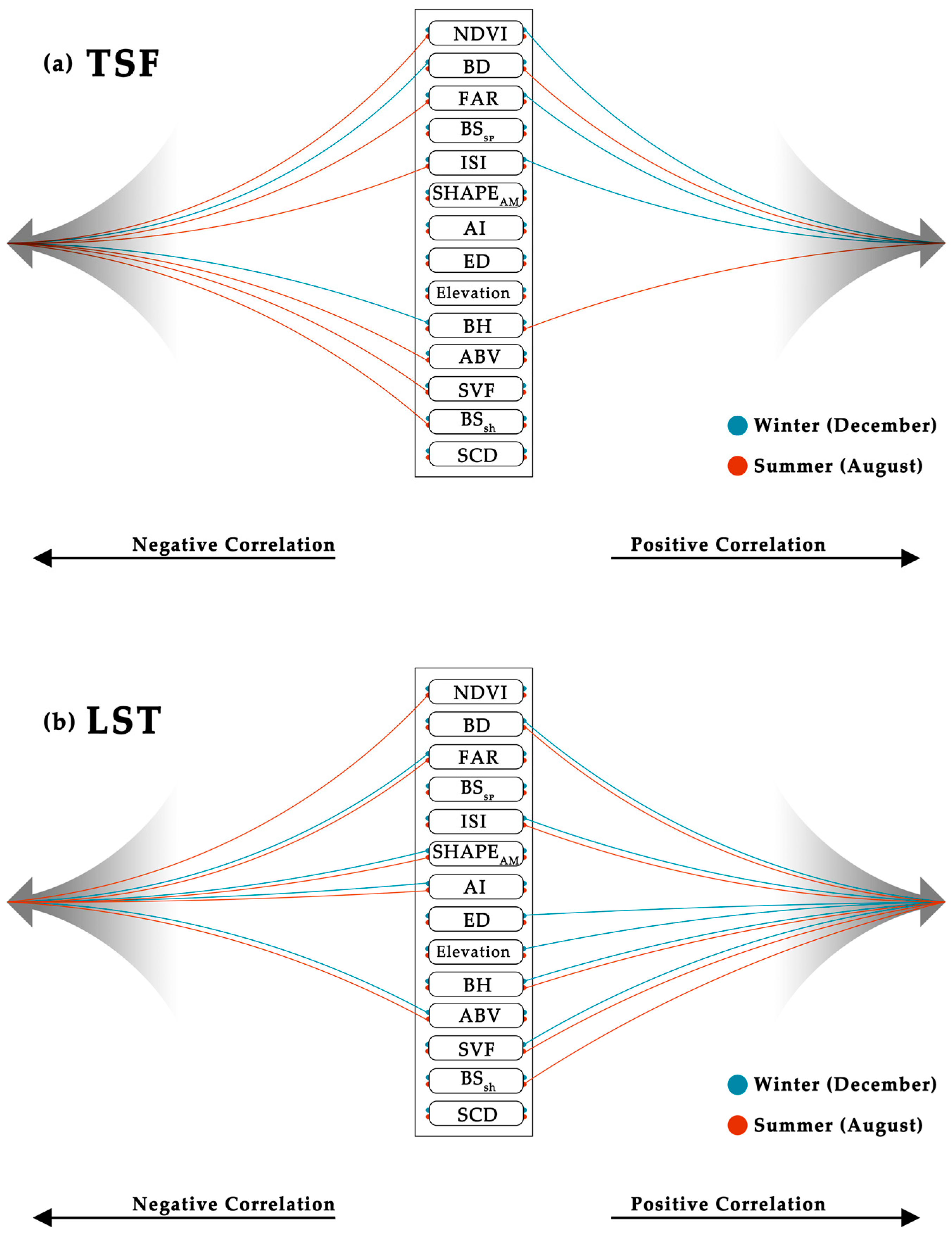
4.3.1. Results of the UM Variables with the TSF OLS Model

We incorporated UM variables and the TSF dataset of the central urban area of Shanghai into the OLS model. The OLS results are presented in Table 3. BD, BH, and TSF exhibit significant positive effects during summer, suggesting that higher building density and height intensify residents’ heat perception. Conversely, NDVI, FAR, SVF, ABV, and TSF demonstrate significant negative effects, implying that expanding urban green spaces and maintaining a more open urban environment can mitigate heat perception. These findings align with theoretical studies on urban ventilation, greening, and cooling during summer. Additionally, BSsh and TSF show significant negative correlations. The negative association of BSsh suggests that as the shape index of buildings increases, residents’ thermal perception decreases. A higher shape index typically reflects more complex, multi-boundary, or irregular building profiles, which may enhance local ventilation, increase shadowed areas, or alter near-surface heat exchange characteristics, thereby alleviating heat perception. Similarly, ISI and TSF also exhibit a significant negative correlation, which contradicts conventional studies.
In winter, FAR, NDVI, and ISI show a significant positive relationship with TSF, indicating that higher building density, increased vegetation cover, and a greater proportion of hard surfaces contribute to a warmer perception among the population. In contrast, BH, BD, and TSF display a significant negative correlation, suggesting that high-rise buildings and densely packed structures may reduce outdoor warmth, potentially by obstructing sunlight. This phenomenon can likely be attributed to the venturi effect, which occurs when air flows through constricted spaces between tall buildings, causing accelerated airflow and significantly increased wind speeds. These conditions subsequently reduce pedestrians’ perception of warmth and thermal comfort outdoors [66].

4.3.2. Results of the UM Variables with the LST OLS Model

We investigated the relationship between UM form and LST in the central urban area of Shanghai using an OLS model (see Table 4).
During summer, BD, BH, SVF, BSsh, and ISI exhibit significant positive effects on surface temperature. This suggests that a dense, high-rise built environment and a high proportion of impervious surfaces exacerbate the urban thermal environment. In contrast, FAR, NDVI, ABV, AI, and SHAPEAM show significant negative correlations with LST, implying that higher plot ratios, greater green coverage, and higher land surface aggregation can mitigate urban heat to some extent. However, the correlation between LST and NDVI in summer is not statistically significant, which contradicts findings from most existing studies.
In winter, BD, BH, SVF, ISI, ED, and elevation demonstrate significant positive effects on LST, indicating that denser and taller buildings, along with increased surface roughness, contribute to higher winter temperatures. Conversely, FAR, ABV, SHAPEAM, and AI exhibit significant negative correlations with winter LST, suggesting that higher plot ratios, greater building volumes, and more compact urban forms help moderate cold-season surface temperatures.

5. Discussion

5.1. The Effect of UM Variables on UTE

Using an OLS model, we analyzed the diverse correlations between UM variables, TSF, and LST (see Figure 6). Regarding TSF, in summer, multiple UM variables significantly influence TSF. Specifically, NDVI, FAR, SVF, ABV, BSsh, and ISI exhibit significant negative correlations with TSF, indicating that increases in these factors reduce residents’ heat perception. Conversely, BD and BH show significant positive effects, suggesting that higher building density and height intensify heat perception. The negative correlation between ISI and TSF transcends conventional understanding. Given that the correlation between NDVI and LST in this study is also insignificant, it suggests that deeper microclimatic and surface material factors may be influencing the pronounced UTE in the central urban area of Shanghai. The relationship between SVF and TSF deviates from traditional assumptions, as low SVF is generally believed to provide shading effects [67]. However, spaces with high SVF tend to experience faster air circulation but also stronger solar radiation, leading to an opposite effect on TSF [68]. This suggests the existence of a threshold in the relationship between SVF and TSF. Previous studies have demonstrated that the impact of SVF on LST is often determined by a threshold, where beyond a certain value, the effect becomes negative [69]. For instance, while SVF generally exhibits a positive correlation with LST, when its value ranges between 0.75 and 1.00, the relationship follows a linear trend. However, for values below 0.75, the correlation weakens significantly [70]. A similar threshold effect is observed in the relationship between BD, BH, SCD, FAR, and LST [69,71,72]. Whether such thresholds exist in the correlation between UM variables and TSF remains uncertain. In winter, TSF is influenced by several UM variables, primarily in the form of cold perception (negative TSF values in this study). FAR, NDVI, ISI, and TSF demonstrate significant positive correlations, whereas BH and BD show significant negative correlations. According to traditional studies, a higher NDVI is generally associated with a more pronounced cooling effect and light obstruction during winter. However, this contradicts the findings of the present study. This discrepancy may be attributed to the fact that in warmer winter months, individuals are more likely to engage in outdoor activities on grassy areas and express positive sentiments regarding the mild climate. This indicates that NDVI, FAR, and ISI improve thermal comfort within appropriate limits, while higher BD and BH decrease comfort. The phenomenon manifests as the urban canyon effect, impeding heat dissipation, while in winter, it shifts to the Venturi effect, amplifying surface wind speed.
Regarding LST, our findings largely align with existing literature, with the primary discrepancy being the non-significant correlation between NDVI and LST in summer. Generally, vegetation is expected to reduce LST in summer but exhibits a positive correlation in winter [36,68,73], which is consistent with its effect on TSF. This discrepancy may stem from factors such as urban microclimate variations and seasonal changes in vegetation cover in the central urban area of Shanghai. In summary, the summer thermal environment is primarily influenced by high-density buildings and impervious surfaces, which exacerbate the UHI effect by increasing solar radiation absorption and heat retention, thereby raising LST and leading to extreme TSF occurrences. Vegetation cover effectively mitigates UTE through transpiration and shading mechanisms. In winter, a dual mechanism is observed: high building density, building height, and sky view limitation restrict long-wave radiation diffusion [70], while moderate plot ratios and landscape complexity enhance surface turbulent exchange, forming thermal diffusion channels that promote winter warm perception [74].
Existing studies on the correlation between UM variables and UTE have integrated both two-dimensional and three-dimensional indicators. Common 2D indicators encompass urban land use patterns, surface attributes, and landscape ecology metrics. In addition to NDVI, BD, FAR, BSsh, ISI, SHAPEAM, AI, and ED examined in this study, frequently used variables include Mean Architecture Projection Area (MAPA), Patch Density (PD), Largest Patch Index (LPI), Shannon’s Diversity Index (SHDI), and Open Space Ratio (OSR) in city-scale studies [34,51,53,75]. These 2D UM variables influence energy exchange efficiency, thereby affecting surface heat flux and significantly altering UTE [76]. The 3D indicators primarily describe architectural morphology. In addition to elevation, BH, ABV, SVF, BSsh, and SCD analyzed in this study, relevant research has incorporated the Mean Compactness Factor (MCF), Average Building Height Standard Deviation (AHSD), Facade Area Index (FAI), and Urban Canyon Ratio (UCR) [34,45,77,78]. Some studies suggest that LST variations in summer are primarily driven by 3D building indices, while winter LST is more strongly associated with 2D land use indices [79]. However, other studies report conflicting conclusions [55], though generally, 3D UM variables exert a greater thermal effect [77]. Moreover, UM variables are closely linked to urban microclimate conditions. Specifically, four key climate indicators—actual temperature, relative humidity, solar radiation, and wind environment—are directly influenced by UM variables, ultimately shaping UTE patterns [80,81]. Given the complexity of urban spatial morphology’s influence on LST, comprehensively evaluating the impact of UM variables on UTE remains a challenging and intricate task.

5.2. Mechanism of Different Effects of UM on TSF and LST

Our research suggests that effective UTE management requires a dual focus on both physical cooling strategies and human-centered design to enhance outdoor thermal comfort [27]. LST is governed by the surface energy balance, whereas human thermal comfort is influenced by atmospheric and physiological processes. LST reflects the temperature of surfaces, including buildings, and is primarily determined by solar radiation, surface materials, and geometric structures. In contrast, TSF represents subjective human thermal perception, which depends on environmental factors such as air temperature, humidity, wind speed, and mean radiant temperature. From a causal perspective, UM affects human thermal perception primarily by altering radiation exposure and wind flow, an indirect influence mediated by atmospheric conditions. When evaluating UTE through both TSF and LST, the following scenarios emerge: High-rise buildings may reduce LST while simultaneously decreasing street-level wind speed. In low-wind environments, even if surface temperatures are relatively cool, individuals may still experience heat stress due to limited evaporative cooling. This phenomenon explains why some UM variables in our study exhibited weaker correlations with TSF compared to LST. Moreover, human thermal perception is influenced by additional factors, including wind patterns, which depend on street orientation and building layout—elements that play a minimal role in LST but are critical for TSF. Consequently, remote sensing of surface temperatures alone is insufficient for assessing livable thermal comfort in urban streetscapes. Conversely, subjective thermal perception data, such as human-body questionnaires, should be supplemented with objective heat distribution measurements for a comprehensive assessment [67]. Comparing these two levels of analysis allows us to infer distinct mechanisms underlying UTE regulation. In summary, UM serves as a fundamental lever in UTE management, facilitating holistic urban microclimate optimization by influencing both LST and TSF. Ultimately, this integrated approach enhances urban climate livability and promotes sustainable urban development.

5.3. Limitations and Shortcomings

This study explores the use of text-based comments on TSF from microblog check-in data as a novel approach to characterizing the UTE. While this method holds significant research value in both process and outcome, it also presents several limitations. First, the comment data primarily capture surface-level semantics in the publisher’s text, whereas deeper semantic interpretation often requires consideration of contextual factors such as environment, clothing, and emotions, which cannot be fully inferred from simple discourse alone. Second, as a major tourist destination, Shanghai is expected to receive 120 million visitors in 2024. Foreign tourists often exhibit varying sensitivities, tolerances, and perception thresholds regarding extreme temperatures, as they may not be fully acclimated to Shanghai’s climate. Consequently, their TSF expressions on social media are strongly influenced by individual subjective experiences. Additionally, tourists’ thermal perception often differs significantly from that of residents [26]. Finally, the findings indicate that the OLS model has limitations in explaining the relationship between UM, LST, and TSF, suggesting that more suitable methodologies should be explored in future research. Moving forward, we aim to further quantify the dynamic relationship between morphological indicators and individual thermal perception, as well as investigate cross-scale collaborative optimization mechanisms.

6. Conclusions

In this study, the OLS model was employed to examine the relationship between LST, TSF, and UTE representation modes, alongside UM variables. The findings provide preliminary evidence that UM regulates UTE by influencing both LST and TSF. From a physical perspective, UM determines how the urban underlying surface absorbs, stores, and releases heat. From a human perception standpoint, UM shapes microclimatic conditions and pedestrian comfort. The study yields three key conclusions: (1) NDVI, BD, FAR, ISI, BH, ABV, SVF, and BSsh significantly explain TSF, whereas SHAPEAM, AI, ED, elevation, BSsp, and SCD show no correlation with TSF. (2) Significant variables, including NDVI, FAR, ISI, UM, BD, and BH, exhibited opposite effects on cold perception in winter compared to heat perception in summer, indicating a consistent influence on thermal perception across seasons. (3) In summer, the significant variables SVF, BSsh, and ISI exhibit opposing effects on TSF and LST. In contrast, during winter, the significant variable FAR demonstrates opposite influences on TSF and LST. These findings suggest that higher building density and height intensify residents’ heat perception and contribute to increased LST. Enhancing urban green spaces and maintaining more open urban environments are effective in mitigating heat perception. The study’s in-depth examination of TSF highlights the importance of human-centered urban planning. Specifically, cooling strategies should not focus solely on reducing LST while overlooking pedestrian activity patterns, as this may lead to an overestimation of actual thermal comfort improvements. Instead, urban planning and behavioral science must jointly account for individuals’ dynamic spatial adaptations. This perspective clarifies the discrepancies between TSF and LST, guiding more comprehensive and effective urban green infrastructure strategies to enhance the UTE.

Author Contributions

Conceptualization, H.Q., F.Z., and B.Q.; methodology, H.Q., M.W., and S.Z.; software, H.Q., M.W., and S.Z.; validation, H.Q., M.W., S.Z., F.Z., and B.Q.; formal analysis, S.Z.; investigation, H.Q., S.Z., and M.W.; resources, F.Z. and B.Q.; data curation, H.Q. and S.Z.; writing—original draft preparation, H.Q., S.Z., M.W., F.Z., and B.Q.; writing—review and editing, F.Z., B.Q., H.Q., S.Z., and M.W.; visualization, M.W.; supervision, F.Z. and B.Q.; project administration, F.Z. and B.Q.; funding acquisition, F.Z. and B.Q. All authors have read and agreed to the published version of the manuscript.

Funding

Sponsored by the Seventh Jiangsu 333 High-level Talent Programme Phase Third-tier Cultivation Candidates Project (2024), the National Natural Science Foundation of China (NSFC) General Project (31971721) and the Priority Academic Program Development of Jiangsu Higher Education Institutions (PAPD).

Data Availability Statement

The research data are available upon request from the corresponding author.

Acknowledgments

We express our gratitude to the United States Geological Survey (USGS) for providing free access to Landsat data. We also acknowledge the Resource and Environmental Science Data Platform of the Institute of Geographic Sciences and Natural Resources Research, Chinese Academy of Sciences, for offering free vector data on buildings in central Shanghai. Additionally, we thank Geospatial Data Cloud (http://www.gscloud.cn/ (accessed on 28 February 2025)) for providing free online Digital Elevation Model (DEM) data for central Shanghai.

Conflicts of Interest

The authors declare no conflicts of interest.

References

  1. Wang, Y.; Chen, L.; Kubota, J. The Relationship between Urbanization, Energy Use and Carbon Emissions: Evidence from a Panel of Association of Southeast Asian Nations (ASEAN) Countries. J. Clean. Prod. 2016, 112, 1368–1374. [Google Scholar] [CrossRef]
  2. Coutts, A.M.; Harris, R.J.; Phan, T.; Livesley, S.J.; Williams, N.S.G.; Tapper, N.J. Thermal Infrared Remote Sensing of Urban Heat: Hotspots, Vegetation, and an Assessment of Techniques for Use in Urban Planning. Remote Sens. Environ. 2016, 186, 637–651. [Google Scholar] [CrossRef]
  3. Zhao, J.; Guo, F.; Zhang, H.; Dong, J. Mechanisms of Non-Stationary Influence of Urban Form on the Diurnal Thermal Environment Based on Machine Learning and MGWR Analysis. Sustain. Cities Soc. 2024, 101, 105194. [Google Scholar] [CrossRef]
  4. Patel, S.; Indraganti, M.; Jawarneh, R.N. A Comprehensive Systematic Review: Impact of Land Use/Land Cover (LULC) on Land Surface Temperatures (LST) and Outdoor Thermal Comfort. Build. Environ. 2024, 249, 111130. [Google Scholar] [CrossRef]
  5. Mirzaei, P.A. Recent Challenges in Modeling of Urban Heat Island. Sustain. Cities Soc. 2015, 19, 200–206. [Google Scholar] [CrossRef]
  6. Aynsley, R.; Spruill, M. Thermal Comfort Models for Outdoor Thermal Comfort in Warm Humid Climates and Probabilities of Low Wind Speeds. J. Wind Eng. Ind. Aerodyn. 1990, 36, 481–488. [Google Scholar] [CrossRef]
  7. Höppe, P. Different Aspects of Assessing Indoor and Outdoor Thermal Comfort. Energy Build. 2002, 34, 661–665. [Google Scholar] [CrossRef]
  8. Nikolopoulou, M.; Steemers, K. Thermal Comfort and Psychological Adaptation as a Guide for Designing Urban Spaces. Energy Build. 2003, 35, 95–101. [Google Scholar] [CrossRef]
  9. Ng, E.; Cheng, V. Urban Human Thermal Comfort in Hot and Humid Hong Kong. Energy Build. 2012, 55, 51–65. [Google Scholar] [CrossRef]
  10. ASHRAE 55-1992; Thermal Environmental Conditions for Human Occupancy. American Society of Heating, Refrigerating and Air-conditioning Engineers Inc.: Atlanta, GA, USA, 1992.
  11. Alghamdi, S.; Tang, W.; Kanjanabootra, S.; Alterman, D. Field Investigations on Thermal Comfort in University Classrooms in New South Wales, Australia. Energy Rep. 2023, 9, 63–71. [Google Scholar] [CrossRef]
  12. Kim, J.; Zhou, Y.; Schiavon, S.; Raftery, P.; Brager, G. Personal Comfort Models: Predicting Individuals’ Thermal Preference Using Occupant Heating and Cooling Behavior and Machine Learning. Build. Environ. 2018, 129, 96–106. [Google Scholar] [CrossRef]
  13. ISO 7730; Moderate Thermal Environment, Determination of PMV and PPD Indices and Specification of the Condition for Thermal Comfort. International Organization for Standardization: Geneva, Switzerland, 1994.
  14. Kumar, P.; Sharma, A. Study on Importance, Procedure, and Scope of Outdoor Thermal Comfort—A Review. Sustain. Cities Soc. 2020, 61, 102297. [Google Scholar] [CrossRef]
  15. Kántor, N.; Égerházi, L.; Unger, J. Subjective Estimation of Thermal Environment in Recreational Urban Spaces—Part 1: Investigations in Szeged, Hungary. Int. J. Biometeorol. 2012, 56, 1075–1088. [Google Scholar] [CrossRef] [PubMed]
  16. Mirzabeigi, S.; Khalili Nasr, B.; Mainini, A.G.; Blanco Cadena, J.D.; Lobaccaro, G. Tailored WBGT as a Heat Stress Index to Assess the Direct Solar Radiation Effect on Indoor Thermal Comfort. Energy Build. 2021, 242, 110974. [Google Scholar] [CrossRef]
  17. Kumar, P.; Sharma, A. Assessing Outdoor Thermal Comfort Conditions at an Urban Park during Summer in the Hot Semi-Arid Region of India. Mater. Today Proc. 2022, 61, 356–369. [Google Scholar] [CrossRef]
  18. Bröde, P.; Krüger, E.L.; Rossi, F.A.; Fiala, D. Predicting Urban Outdoor Thermal Comfort by the Universal Thermal Climate Index UTCI—A Case Study in Southern Brazil. Int. J. Biometeorol. 2012, 56, 471–480. [Google Scholar] [CrossRef]
  19. Mahdavinejad, M.; Shaeri, J.; Nezami, A.; Goharian, A. Comparing Universal Thermal Climate Index (UTCI) with Selected Thermal Indices to Evaluate Outdoor Thermal Comfort in Traditional Courtyards with BWh Climate. Urban Clim. 2024, 54, 101839. [Google Scholar] [CrossRef]
  20. Sharmin, T.; Steemers, K.; Humphreys, M. Outdoor Thermal Comfort and Summer PET Range: A Field Study in Tropical City Dhaka. Energy Build. 2019, 198, 149–159. [Google Scholar] [CrossRef]
  21. Ugursal, A.; Culp, C. Gender Differences of Thermal Comfort Perception UnderTransient Environmental and Metabolic Conditions—ProQuest. ASHRAE Trans. 2013, 119, 52–62. [Google Scholar]
  22. Xiong, J.; Lian, Z.; Zhou, X.; You, J.; Lin, Y. Effects of Temperature Steps on Human Health and Thermal Comfort. Build. Environ. 2015, 94, 144–154. [Google Scholar] [CrossRef]
  23. Nkurikiyeyezu, K.N.; Suzuki, Y.; Lopez, G.F. Heart Rate Variability as a Predictive Biomarker of Thermal Comfort. J. Ambient. Intell. Hum. Comput. 2018, 9, 1465–1477. [Google Scholar] [CrossRef]
  24. Xiong, J.; Lian, Z.; Zhang, H. Physiological Response to Typical Temperature Step-Changes in Winter of China. Energy Build. 2017, 138, 687–694. [Google Scholar] [CrossRef]
  25. Nikolopoulou, M.; Baker, N.; Steemers, K. Thermal Comfort in Outdoor Urban Spaces: Understanding the Human Parameter. Sol. Energy 2001, 70, 227–235. [Google Scholar] [CrossRef]
  26. Lindner-Cendrowska, K.; Błażejczyk, K. Impact of Selected Personal Factors on Seasonal Variability of Recreationist Weather Perceptions and Preferences in Warsaw (Poland). Int. J. Biometeorol. 2018, 62, 113–125. [Google Scholar] [CrossRef]
  27. Villadiego, K.; Velay-Dabat, M.A. Outdoor Thermal Comfort in a Hot and Humid Climate of Colombia: A Field Study in Barranquilla. Build. Environ. 2014, 75, 142–152. [Google Scholar] [CrossRef]
  28. Ge, J.; Wu, J.; Chen, S.; Wu, J. Energy Efficiency Optimization Strategies for University Research Buildings with Hot Summer and Cold Winter Climate of China Based on the Adaptive Thermal Comfort. J. Build. Eng. 2018, 18, 321–330. [Google Scholar] [CrossRef]
  29. Aghniaey, S.; Lawrence, T.M.; Sharpton, T.N.; Douglass, S.P.; Oliver, T.; Sutter, M. Thermal Comfort Evaluation in Campus Classrooms during Room Temperature Adjustment Corresponding to Demand Response. Build. Environ. 2019, 148, 488–497. [Google Scholar] [CrossRef]
  30. Arens, E.; Humphreys, M.A.; de Dear, R.; Zhang, H. Are ‘Class A’ Temperature Requirements Realistic or Desirable? Build. Environ. 2010, 45, 4–10. [Google Scholar] [CrossRef]
  31. Hoyt, T.; Lee, K.H.; Zhang, H.; Arens, E.; Webster, T. Energy Savings from Extended Air Temperature Setpoints and Reductions in Room Air Mixing; UC Berkeley: Berkeley, CA, USA, 2005. [Google Scholar]
  32. Humphreys, M.A.; Hancock, M. Do People like to Feel ‘Neutral’?: Exploring the Variation of the Desired Thermal Sensation on the ASHRAE Scale. Energy Build. 2007, 39, 867–874. [Google Scholar] [CrossRef]
  33. Fox, R.H.; Woodward, P.M.; Exton-Smith, A.N.; Green, M.F.; Donnison, D.V.; Wicks, M.H. Body Temperatures in the Elderly: A National Study of Physiological, Social and Environmental Conditions. Br. Med. J. 1973, 1, 200–206. [Google Scholar] [CrossRef]
  34. Yuan, B.; Zhou, L.; Hu, F.; Wei, C. Effects of 2D/3D Urban Morphology on Land Surface Temperature: Contribution, Response, and Interaction. Urban Clim. 2024, 53, 101791. [Google Scholar] [CrossRef]
  35. Liu, Y.; Peng, J.; Wang, Y. Efficiency of Landscape Metrics Characterizing Urban Land Surface Temperature. Landsc. Urban Plan. 2018, 180, 36–53. [Google Scholar] [CrossRef]
  36. Peng, J.; Jia, J.; Liu, Y.; Li, H.; Wu, J. Seasonal Contrast of the Dominant Factors for Spatial Distribution of Land Surface Temperature in Urban Areas. Remote Sens. Environ. 2018, 215, 255–267. [Google Scholar] [CrossRef]
  37. Li, J.; Wang, F.; Fu, Y.; Guo, B.; Zhao, Y.; Yu, H. A Novel SUHI Referenced Estimation Method for Multicenters Urban Agglomeration Using DMSP/OLS Nighttime Light Data. IEEE J. Sel. Top. Appl. Earth Obs. Remote Sens. 2020, 13, 1416–1425. [Google Scholar] [CrossRef]
  38. Liu, D.; Chen, N.; Zhang, X.; Wang, C.; Du, W. Annual Large-Scale Urban Land Mapping Based on Landsat Time Series in Google Earth Engine and OpenStreetMap Data: A Case Study in the Middle Yangtze River Basin. ISPRS J. Photogramm. Remote Sens. 2020, 159, 337–351. [Google Scholar] [CrossRef]
  39. Geletič, J.; Lehnert, M.; Savić, S.; Milošević, D. Inter-/Intra-Zonal Seasonal Variability of the Surface Urban Heat Island Based on Local Climate Zones in Three Central European Cities. Build. Environ. 2019, 156, 21–32. [Google Scholar] [CrossRef]
  40. Stewart, I.D.; Oke, T.R. Local Climate Zones for Urban Temperature Studies. Bull. Am. Meteorol. Soc. 2012, 93, 1879–1900. [Google Scholar] [CrossRef]
  41. Oke, T.R. Towards Better Scientific Communication in Urban Climate. Theor. Appl. Climatol. 2006, 84, 179–190. [Google Scholar] [CrossRef]
  42. Chen, S.; He, P.; Yu, B.; Wei, D.; Chen, Y. The Challenge of Noise Pollution in High-Density Urban Areas: Relationship between 2D/3D Urban Morphology and Noise Perception. Build. Environ. 2024, 253, 111313. [Google Scholar] [CrossRef]
  43. Guo, F.; Schlink, U.; Wu, W.; Hu, D.; Sun, J. Scale-Dependent and Season-Dependent Impacts of 2D/3D Building Morphology on Land Surface Temperature. Sustain. Cities Soc. 2023, 97, 104788. [Google Scholar] [CrossRef]
  44. Fotheringham, A.S.; Wong, D.W.S. The Modifiable Areal Unit Problem in Multivariate Statistical Analysis. Environ. Plan A 1991, 23, 1025–1044. [Google Scholar] [CrossRef]
  45. Han, W. Analyzing the Scale Dependent Effect of Urban Building Morphology on Land Surface Temperature Using Random Forest Algorithm. Sci. Rep. 2023, 13, 19312. [Google Scholar] [CrossRef]
  46. Weng, Q.; Lu, D.; Schubring, J. Estimation of Land Surface Temperature–Vegetation Abundance Relationship for Urban Heat Island Studies. Remote Sens. Environ. 2004, 89, 467–483. [Google Scholar] [CrossRef]
  47. Li, X.; Zhou, W.; Ouyang, Z. Relationship between Land Surface Temperature and Spatial Pattern of Greenspace: What Are the Effects of Spatial Resolution? Landsc. Urban Plan. 2013, 114, 1–8. [Google Scholar] [CrossRef]
  48. Niu, H.; Silva, E.A. Crowdsourced Data Mining for Urban Activity: Review of Data Sources, Applications, and Methods. J. Urban Plan. Dev. 2020, 146, 04020007. [Google Scholar] [CrossRef]
  49. Chen, Y.; Niu, H.; Silva, E.A. The Road to Recovery: Sensing Public Opinion towards Reopening Measures with Social Media Data in Post-Lockdown Cities. Cities 2023, 132, 104054. [Google Scholar] [CrossRef]
  50. Wang, Z.; Zhou, R.; Yu, Y. The Impact of Urban Morphology on Land Surface Temperature under Seasonal and Diurnal Variations: Marginal and Interaction Effects. Build. Environ. 2025, 272, 112673. [Google Scholar] [CrossRef]
  51. Yelixiati, H.; Tong, L.; Luo, S.; Chen, Z. Spatiotemporal Heterogeneity of the Relationship between Urban Morphology and Land Surface Temperature at a Block Scale. Sustain. Cities Soc. 2024, 113, 105711. [Google Scholar] [CrossRef]
  52. Wen, D.; Wang, L.; Cao, Q.; Hong, M.; Wang, H.; Bian, G. A Comparative Study of the Effects of Urban Morphology on Land Surface Temperature in Chengdu and Chongqing, China. Sci. Rep. 2024, 14, 25130. [Google Scholar] [CrossRef]
  53. Zhou, L.; Hu, F.; Wang, B.; Wei, C.; Sun, D.; Wang, S. Relationship between Urban Landscape Structure and Land Surface Temperature: Spatial Hierarchy and Interaction Effects. Sustain. Cities Soc. 2022, 80, 103795. [Google Scholar] [CrossRef]
  54. Yin, C.; Yuan, M.; Lu, Y.; Huang, Y.; Liu, Y. Effects of Urban Form on the Urban Heat Island Effect Based on Spatial Regression Model. Sci. Total Environ. 2018, 634, 696–704. [Google Scholar] [CrossRef] [PubMed]
  55. Hu, Y.; Dai, Z.; Guldmann, J.-M. Modeling the Impact of 2D/3D Urban Indicators on the Urban Heat Island over Different Seasons: A Boosted Regression Tree Approach. J. Environ. Manag. 2020, 266, 110424. [Google Scholar] [CrossRef] [PubMed]
  56. Wu, Y.; Che, Y.; Liao, W.; Liu, X. The Impact of Urban Morphology on Land Surface Temperature across Urban-Rural Gradients in the Pearl River Delta, China. Build. Environ. 2025, 267, 112215. [Google Scholar] [CrossRef]
  57. Fanger, P.O. Thermal Comfort; Danish Technical Press: Copenhagen, Denmark, 1970. [Google Scholar]
  58. Fleiss, J.L.; Cohen, J. The Equivalence of Weighted Kappa and the Intraclass Correlation Coefficient as Measures of Reliability. Educ. Psychol. Meas. 1973, 33, 613–619. [Google Scholar] [CrossRef]
  59. Morabito, M.; Crisci, A.; Messeri, A.; Orlandini, S.; Raschi, A.; Maracchi, G.; Munafò, M. The Impact of Built-up Surfaces on Land Surface Temperatures in Italian Urban Areas. Sci. Total Environ. 2016, 551–552, 317–326. [Google Scholar] [CrossRef]
  60. Deilami, K.; Kamruzzaman, M.; Liu, Y. Urban Heat Island Effect: A Systematic Review of Spatio-Temporal Factors, Data, Methods, and Mitigation Measures. Int. J. Appl. Earth Obs. Geoinf. 2018, 67, 30–42. [Google Scholar] [CrossRef]
  61. Gao, Y.; Zhao, J.; Han, L. Exploring the Spatial Heterogeneity of Urban Heat Island Effect and Its Relationship to Block Morphology with the Geographically Weighted Regression Model. Sustain. Cities Soc. 2022, 76, 103431. [Google Scholar] [CrossRef]
  62. Li, L.; Zha, Y.; Zhang, J. Spatially Non-Stationary Effect of Underlying Driving Factors on Surface Urban Heat Islands in Global Major Cities. Int. J. Appl. Earth Obs. Geoinf. 2020, 90, 102131. [Google Scholar] [CrossRef]
  63. Yu, H.; Peng, Z.-R. Exploring the Spatial Variation of Ridesourcing Demand and Its Relationship to Built Environment and Socioeconomic Factors with the Geographically Weighted Poisson Regression. J. Transp. Geogr. 2019, 75, 147–163. [Google Scholar] [CrossRef]
  64. Anselin, L. Local Indicators of Spatial Association—LISA. Geogr. Anal. 1995, 27, 93–115. [Google Scholar] [CrossRef]
  65. Wheeler, D.; Tiefelsdorf, M. Multicollinearity and Correlation among Local Regression Coefficients in Geographically Weighted Regression. J. Geogr. Syst. 2005, 7, 161–187. [Google Scholar] [CrossRef]
  66. Nugroho, N.Y.; Triyadi, S.; Wonorahardjo, S. Effect of High-Rise Buildings on the Surrounding Thermal Environment. Build. Environ. 2022, 207, 108393. [Google Scholar] [CrossRef]
  67. He, X.; Miao, S.; Shen, S.; Li, J.; Zhang, B.; Zhang, Z.; Chen, X. Influence of Sky View Factor on Outdoor Thermal Environment and Physiological Equivalent Temperature. Int. J. Biometeorol. 2015, 59, 285–297. [Google Scholar] [CrossRef] [PubMed]
  68. Xiang, Y.; Huang, C.; Huang, X.; Zhou, Z.; Wang, X. Seasonal Variations of the Dominant Factors for Spatial Heterogeneity and Time Inconsistency of Land Surface Temperature in an Urban Agglomeration of Central China. Sustain. Cities Soc. 2021, 75, 103285. [Google Scholar] [CrossRef]
  69. Han, D.; An, H.; Wang, F.; Xu, X.; Qiao, Z.; Wang, M.; Sui, X.; Liang, S.; Hou, X.; Cai, H.; et al. Understanding Seasonal Contributions of Urban Morphology to Thermal Environment Based on Boosted Regression Tree Approach. Build. Environ. 2022, 226, 109770. [Google Scholar] [CrossRef]
  70. Scarano, M.; Sobrino, J.A. On the Relationship between the Sky View Factor and the Land Surface Temperature Derived by Landsat-8 Images in Bari, Italy. Int. J. Remote Sens. 2015, 36, 4820–4835. [Google Scholar] [CrossRef]
  71. Wang, J.; Meng, F.; Lu, H.; Lv, Y.; Jing, T. Individual and Combined Effects of 3D Buildings and Green Spaces on the Urban Thermal Environment: A Case Study in Jinan, China. Atmosphere 2023, 14, 908. [Google Scholar] [CrossRef]
  72. Li, J.; Song, C.; Cao, L.; Zhu, F.; Meng, X.; Wu, J. Impacts of Landscape Structure on Surface Urban Heat Islands: A Case Study of Shanghai, China. Remote Sens. Environ. 2011, 115, 3249–3263. [Google Scholar] [CrossRef]
  73. Sun, D.; Kafatos, M. Note on the NDVI-LST Relationship and the Use of Temperature-Related Drought Indices over North America. Geophys. Res. Lett. 2007, 34. [Google Scholar] [CrossRef]
  74. Wu, Z.; Tong, Z.; Wang, M.; Long, Q. Assessing the Impact of Urban Morphological Parameters on Land Surface Temperature in the Heat Aggregation Areas with Spatial Heterogeneity: A Case Study of Nanjing. Build. Environ. 2023, 235, 110232. [Google Scholar] [CrossRef]
  75. Nasar-u-Minallah, M.; Haase, D.; Qureshi, S. Evaluating the Impact of Landscape Configuration, Patterns and Composition on Land Surface Temperature: An Urban Heat Island Study in the Megacity Lahore, Pakistan. Environ. Monit. Assess. 2024, 196, 627. [Google Scholar] [CrossRef] [PubMed]
  76. Liu, H.; Weng, Q. Seasonal Variations in the Relationship between Landscape Pattern and Land Surface Temperature in Indianapolis, USA. Environ. Monit. Assess. 2008, 144, 199–219. [Google Scholar] [CrossRef] [PubMed]
  77. Li, H.; Li, Y.; Wang, T.; Wang, Z.; Gao, M.; Shen, H. Quantifying 3D Building Form Effects on Urban Land Surface Temperature and Modeling Seasonal Correlation Patterns. Build. Environ. 2021, 204, 108132. [Google Scholar] [CrossRef]
  78. Coseo, P.; Larsen, L. How Factors of Land Use/Land Cover, Building Configuration, and Adjacent Heat Sources and Sinks Explain Urban Heat Islands in Chicago. Landsc. Urban Plan. 2014, 125, 117–129. [Google Scholar] [CrossRef]
  79. Yan, J.; Yin, C.; An, Z.; Mu, B.; Wen, Q.; Li, Y.; Zhang, Y.; Chen, W.; Wang, L.; Song, Y. The Influence of Urban Form on Land Surface Temperature: A Comprehensive Investigation from 2D Urban Land Use and 3D Buildings. Land 2023, 12, 1802. [Google Scholar] [CrossRef]
  80. Cao, J.; Zhou, W.; Zheng, Z.; Ren, T.; Wang, W. Within-City Spatial and Temporal Heterogeneity of Air Temperature and Its Relationship with Land Surface Temperature. Landsc. Urban Plan. 2021, 206, 103979. [Google Scholar] [CrossRef]
  81. Goldblatt, R.; Addas, A.; Crull, D.; Maghrabi, A.; Levin, G.G.; Rubinyi, S. Remotely Sensed Derived Land Surface Temperature (LST) as a Proxy for Air Temperature and Thermal Comfort at a Small Geographical Scale. Land 2021, 10, 410. [Google Scholar] [CrossRef]
Figure 1. Study area.
Land 14 00769 g001
Figure 2. Spatial information data of central urban area of Shanghai: (a) administrative division; (b) land use type; (c) DEM data; (d) building vector data (building distribution and local building height).
Land 14 00769 g002
Figure 3. Description of the TFOI index generated based on Weibo check-in data represents (a) summer data and (b) winter data.
Land 14 00769 g003
Figure 4. (a) Summer LST and (b) Winter LST of the central urban area of Shanghai derived from Landsat-8 image.
Land 14 00769 g004
Figure 5. Central urban area of Shanghai UM: (a) NDVI; (b) BD; (c) FAR; (d) BSsp; (e) ISI; (f) SHAPEAM; (g) AI; (h) ED; (i) elevation; (j) BH; (k) ABV; (l) SVF; (m) BSsh; (n) SCD.
Land 14 00769 g005
Figure 6. Correlation between the UM variable and TSF and LST. (a) TSF; (b) LST.
Land 14 00769 g006
Table 1. The summary of 2D and 3D metrics in this study.
NormFormulaDescriptionReferences
2D Indicators
N D V I N D V I = ρ n i n ρ r e d ρ n i n + ρ r e d Show the extent of the green space.[51]
B D B D = i = 1 n A i S × 100 % Reflects the extent to which the ground is covered by buildings.[51]
F A R F A R = i = 1 n f i × A i S Characterize the intensity of land development.[42,51]
B S s p B S s p = 1 n i = 1 n d i Average building-to-building distance between buildings in each grid pixel.[42]
I S I I S I = A i m p e r v i o u s A The proportion of impervious surface coverage per unit area.[52]
S H A P E A M S H A P E A M = j = 1 n 0.25 P i j a i j a i j j n a i j Reflecting the complexity of specific types of landscape patch boundaries.[34]
A I A I = i = 1 n   ( g i i m a x ) P i The aggregation characteristics reflecting the distribution of patches.[34,53]
E D E D = j = 1 n e i j A Measure the degree of landscape fragmentation.[34,53]
3D Indicators
ElevationDirectly from DEM dataIndicates the elevation status of the urban space.-
B H Directly from the building vector datasetIndicates the vertical height of the building.[50]
A B V A B V = i n V i n Reflecting the degree of urban intensification.[34]
S V F S V F = 1 i = 1 n sin γ i m Reflects spatial openness.[20,54,55]
B S s h B S s h = P i P i 2 16 S A i 4 The average of the shape indices of all buildings in each grid pixel.[42]
S C D S C D = i = 1 n V i i = 1 n H i Reflects the density of the distribution of elements within the spatial unit.[56]
Note: ρ n i n and ρ r e d are the reflectance values of the near infrared and red channels, respectively. A i , f i , P i , V i , and H i are the area, the number of floors, the perimeter, the volume, and the height, respectively, occupied by the building i or patch i . n denotes the number of buildings, d i is the distance between neighboring buildings, i is the total logarithm between buildings, and A is the area of the unit. γ denotes the elevation angle of the topographic horizon, and m denotes the number of directions used to estimate γ . e i j denotes the length of the edge segment j in the landscape patch of category i . g i i denotes the number of adjacencies between the basic spatial units of the landscape patches of category i , and P i denotes the proportion of the landscape patches of category i in the landscape area.
Table 2. Seven-level TSF scale.
ScaleRulerHuman Perception and Physiological Response
−3ColdSkin tingling, shortness of breath, high risk of core temperature decline.
−2CoolThe limbs are stiff and trembling, and may be frostbitten after exposure for 30 min.
−1Slightly coolHands and feet are slightly cold and can be adjusted independently.
0NeutralNo active regulation behavior, dry skin, stable heart rate.
1Slightly warmSlight sweating and increased thirst.
2WarmContinuous sweating, increased heart rate, and decreased attention.
3HotRisk of heat cramps, and failure of thermoregulation.
Table 3. Results of OLS model on UM and TSF in the central urban area of Shanghai.
VariablesCoef.Std. Err.Tp
Summer (August)
NDVI−12.5013.154−3.9630.013 **
BD22.57811.3231.9940.064 *
FAR−8.8782.496−3.5570.006 ***
BSsp0.0570.0600.9630.307
ISI−11.9252.214−5.3870.001 ***
SHAPEAM−0.2370.164−1.4380.259
AI−0.2200.211−1.0440.207
ED11.66210.7631.0840.334
Elevation0.2180.1751.2460.425
BH4.3771.2413.5270.028 **
ABV−0.0120.007−1.7390.089 *
SVF−18.1378.134−2.2300.039 **
BSsh−0.1790.137−1.3050.086 *
SCD−0.0310.300−0.1030.906
R-squared0.119
Winter (December)
NDVI6.611.7993.6750.041 **
BD−7.9215.235−1.5130.072 *
FAR3.3741.3452.5080.002 ***
BSsp0.0580.0620.9400.137
ISI4.9381.2803.8570.014 **
SHAPEAM0.0270.0950.2890.695
AI0.1460.1181.2360.147
ED−4.5676.359−0.7180.404
Elevation0.0610.0990.6220.491
BH−1.6920.640−2.6450.069 *
ABV−0.0010.004−0.1910.872
SVF6.8384.6781.4620.256
BSsh0.0070.0310.2410.733
SCD−0.1040.161−0.6460.351
R-squared0.081
Note: *** p < 0.01, ** p < 0.05, * p < 0.1.
Table 4. Results of OLS model on UM and LST in the central urban area of Shanghai.
VariablesCoef.Std. Err.tp
Summer (August)
NDVI−1.2880.193−6.6720.000 ***
BD19.7770.59133.4770.000 ***
FAR−2.3350.199−11.7440.000 ***
BSsp−0.0040.008−0.5230.646
ISI2.7040.15018.0490.000 ***
SHAPEAM−0.0250.011−2.350.019 **
AI−0.0430.016−2.7790.006 ***
ED0.0690.5920.1160.907
Elevation0.0110.0120.8860.370
BH1.2980.05125.6530.000 ***
ABV−0.0040.001−6.7060.000 ***
SVF3.7550.7295.1490.000 ***
BSsh0.0580.00511.7650.000 ***
SCD−0.0040.010−0.4530.716
R-squared0.314
Winter (December)
NDVI0.9280.0979.5460.000 ***
BD8.0120.29726.9340.000 ***
FAR−1.1960.100−11.9450.000 ***
BSsp0.0010.0040.1530.893
ISI0.6500.0758.6120.000 ***
SHAPEAM−0.0290.005−5.3320.000 ***
AI−0.0400.008−5.0710.000 ***
ED0.8510.2982.8570.002 ***
Elevation0.0360.0065.7510.000 ***
BH0.3890.02515.2640.000 ***
ABV−0.0030.000−9.1660.000 ***
SVF3.0490.3678.3030.000 ***
BSsh0.0300.00212.3480.000 ***
SCD−0.0120.005−2.3180.029
R-squared0.174
Note: *** p < 0.01, ** p < 0.05.
Disclaimer/Publisher’s Note: The statements, opinions and data contained in all publications are solely those of the individual author(s) and contributor(s) and not of MDPI and/or the editor(s). MDPI and/or the editor(s) disclaim responsibility for any injury to people or property resulting from any ideas, methods, instructions or products referred to in the content.

