Abstract
Rapid urbanization in Kathmandu Valley has strained its aquifer system, causing significant land subsidence. This study employs LiCSBAS for InSAR processing of Sentinel-1 data (2017–2024) to map subsidence-prone areas. The significant subsidence was found in northwest (Baluwatar, Samakhusi, and Manmaiju), southern (Gwarko, Patan, and Koteshwor), and northeast (Madhapur Thimi and Gathhaghar) regions with a maximum subsidence rate ~21 cm/yr. Subsidence has also expanded towards the outskirts and open areas in the eastern and southern parts of Lalitpur and Bhaktapur districts. Emerging hot spot analysis reveals a slowing subsidence trend in high-risk zones, possibly linked to the MWSP project reducing groundwater extraction from 58 MLD (2021) to 26 MLD (2024). Many subsidence-affected areas are located over the Kalimati and Gokarna Formations in highly urbanized areas. The key contributing factors to subsidence are soil compaction, excessive groundwater use, and urban sprawl encroaching open areas and recharge zones. These findings underscore the urgent need for sustainable groundwater management and land-use planning to promote urban resilience.
1. Introduction
Land subsidence (LS) is a pervasive geohazard that presents formidable challenges to urban environments, mainly in densely populated regions such as Asia. This phenomenon is characterized by the gradual downward displacement of the land surface due to excessive groundwater extraction resulting in the compaction of soil layers. The subsequent reduction in pore pressure compromises the soil’s structural integrity, diminishing its capacity to support overlying loads. This elevates the vulnerability of edifices, thoroughfares, and vital infrastructure to damage while amplifying the propensity for urban pluvial inundation, landslides, sinkholes, and an array of cascading geo disaster [1,2,3,4,5]. Many urban cities have suffered land subsidence due to the exploitation of groundwaters, which could potentially impact 29% of total urban population [1,6,7,8,9,10,11,12].
Several major cities, including Prato in Italy, Wuhan in China, Jakarta in Indonesia, and Metro Manila in the Philippines, have reported substantial subsidence due to rapid urbanization and the over-extraction of groundwater resources [13]. Kathmandu Valley (KV), comprising three district areas including the country’s capital city, is a bowl-shaped alluvial basin surrounded by mountains. As a nexus of socioeconomic vitality, political authority, educational advancement, and industrial enterprise, the valley magnetizes substantial rural-to-urban migration, intensifying its urban sprawl. This demographic surge exerts profound pressure on finite resources of groundwater, agriculture land, transportation, residential buildings, and other infrastructures. Surrounded by towering mountains and national parks to the north, KV faces severe spatial constraints for urban expansion, driving extensive encroachment onto riverbanks, open spaces, and cropland. The rapid proliferation of residential structures within the valley is staggering; between the late 1990s and 2021, the number of newly built houses in the 50-square-kilometer Kathmandu Metropolitan City (KMC) surged to 70,090 an alarming figure nearly seven times the area’s sustainable capacity [14]. Lax regulatory oversight and enforcement deficiencies have emboldened unchecked construction activities and widespread groundwater extraction through tube wells, exacerbating environmental degradation. KV is the most densely populated area in the country with a staggering population density of 5169 individuals per square kilometer [15]. Between 2015 and 2024, the demand for water in KV escalated by 36% due to limited water sources and growing urban population. Kathmandu Upatyaka Khanepani Limited (KUKL; the valley’s official water management authority) report shows that groundwater pumping rates increased from 2.3 MLD in 1979 to 29.2 MLD in 1999, peaking at 58.79 MLD in 2021. The rate of groundwater abstraction has surpassed the replenishment rate since the mid-1980s, with this disparity continuing to widen over time. The completion of the Melamchi Water Supply Project (MWSP) and additional sourcing from the Bagmati River has enabled KUKL to increase its water supply to 47% of the total demand (506 MLD) in 2024. This represents a notable advancement over the preceding years where KUKL only managed to supply 28.8% in 2023 and a mere 21% in 2022 [16]. Despite these improvements, frequent landslides and floods disrupt water distribution from MWSP and river sources, leading to prolonged supply shortages and exacerbating Kathmandu Valley’s chronic water deficit. Due to a shortage in water supply, most residents remain dependent on private vendors, third-party water suppliers, and unregulated tube wells depleting the water level up to ~2.5 m annually [17]. Nepal ranks 11th in earthquake vulnerability and 16th for multiple hazards globally as per the United Nation Development program (UNDP) [18]. The most recent seismic disaster of 2015 Gorkha Earthquake (Mw 7.2) caused widespread devastation, inducing substantial liquefaction in KV and damaging critical infrastructure [19]. If a future seismic event strikes with an epicenter near Kathmandu, the ongoing land subsidence will worsen the disaster. It will increase structural collapses and heighten economic losses. Without strategic intervention, the combination of subsidence and seismic hazards endangers the valley’s long-term resilience. This situation demands urgent mitigation measures. These measures must address groundwater depletion and enforce sustainable urban planning policies.
Traditional methods like GNSS and leveling methods are most commonly used technique to precisely measure subsidence worldwide. HoustonNet operates and processes over 250 permanent GNSS stations to monitor subsidence-related hazards with high precision in Houston, Texas [5]. But their prohibitive costs, labor-intensive nature, frequent upkeep demands, and limited spatial coverage render them impractical for widespread adoption in resource-scarce settings like Kathmandu Valley. Recent strides in remote sensing have redefined large-scale geohazard surveillance, proffering cost-efficient, expansive alternatives. Technologies including Unmanned Aerial Vehicles (UAVs), photogrammetry, satellite imagery, Light Detection and Ranging (LiDAR), and Interferometric Synthetic Aperture Radar (InSAR) have demonstrated versatility across domains from disaster relief to ecological oversight and geohazard evaluation. Among these, InSAR has ascended as a pre-eminent tool for discerning slow-evolving geohazards such as glacial shifts, landslides, and subsidence with millimeter-scale fidelity.
Multiple studies have employed InSAR to investigate subsidence in Kathmandu Valley. Bhattarai (2011) pioneered the application of Differential InSAR (DInSAR) using ALOS PALSAR imagery (2007–2010), identifying seven distinct subsidence zones with rates ranging from 1 to 9.9 cm/year [20]. Following the 2015 Gorkha Earthquake (Mw 7.2), Krishna (2018) analyzed 16 ALOS-1 PALSAR and 26 Sentinel-1 A/B SAR data to measure subsidence velocity before and after the event. Their result revealed an increase in subsidence rates from 8.2 cm/year prior to the earthquake to 12 cm/year afterward. This escalation underscores the seismic influence on subsidence dynamics [21]. Kumahara [22] examined four active faults in a field visit on July 2025 (3 months prior to earthquake) and created a detailed DEM from height of 10 m using Agisoft Photoscan Professional. His findings found no evidence of surface ruptures, suggesting persistent, unrelieved tectonic stress that could elevate the risk of future seismic events. Stallin (2017–2019) employed Persistent Scatterer Interferometry (PSI) on descending-orbit SAR datasets and found a maximum subsidence rate of 13 cm/year in the line-of-sight (LOS) direction [23]. More recently, Huang et al. (2024) utilized Small Baseline Subset (SBAS) InSAR techniques on Sentinel-1 data (2015–2021), reporting peak subsidence rates of 20 cm/year. He analyzed the InSAR-derived subsidence rate based on the river channel’s DTM and found that vertical velocity increased with elevation. Their findings showed a reduced subsidence rate in areas near river streams, with seasonal fluctuation in time series providing crucial evidence of connection between shallow aquifers and nearby streams [24].
Research on subsidence in Kathmandu Valley has primarily focused on measuring rates with limited consideration of geological structures, lithological variations, or long-term trends. Many InSAR studies rely on data from either ascending or descending orbits, using line-of-sight displacement to estimate vertical motion. Combining both orbits allows for more accurate vertical displacement measurements. Most existing studies cover less than three years, failing to capture sustained patterns or underlying causes. Given the rapid rate of subsidence and growing seismic risk, continuous monitoring and recalibration of historical data are critical. Spatial variability across different geological formations and land-use zones also requires further investigation. Previous validation efforts have depended on a single GPS station, NAST (27.657, 85.328), which suffers from limited spatial coverage, power outages, and maintenance issues. In this study, we applied Persistent Scatterer InSAR (PS-InSAR), a histogram method, and GPS observations to assess the accuracy and reliability of InSAR-derived results. We processed InSAR data from both ascending and descending orbits from 2017 to 2024 to extract more precise vertical displacement. The two years following the earthquake are excluded as post-seismic relaxation could distort subsidence rates and introduce outliers into the analysis.
Emergency hot spot analysis (EHA) from ESRI is an effective tool for spatiotemporal analysis, facilitating the identification of emerging patterns through comparison with historical data [25]. This approach offers a more efficient alternative to the time-intensive process of examining the time series of thousands of pixels to detect trends. EHA conducts spatiotemporal analysis by constructing a Space–Time Cube (STC) from input data, efficiently isolating statistically significant regions based on their temporal evolution. Shuhab D. Khan et al. (2021) fused EHA with InSAR data (2015–2019) and seismic records to probe the nexus between seismicity and subsidence in Peshawar, Pakistan, pinpointing hot spots in densely populated urban zones where groundwater overexploitation predominated [26]. Similarly, Wei Zhang et al. (2023) integrated EHA with Persistent Scatterer InSAR (PS-InSAR) to investigate settlement patterns in Beijing, uncovering persistent hot spot clusters that signaled latent subsidence foci overlooked by conventional techniques [10]. The versatility of EHA extends beyond subsidence, encompassing time-dependent phenomena such as landslides, epidemiological outbreaks like COVID-19, environmental calamities, and stock market fluctuations. This study pioneers the integration of EHA with LiCSBAS outputs, aiming to discern shifts in subsidence trends within the study area, thereby advancing the analytical framework for geohazard assessment in KV.
The main objective of this study is to (1) examine subsidence in KV and refine existing records with updated findings; (2) find any changing pattern using EHA tool to assess whether governmental interventions have effectively stabilized subsidence rates in specific areas; (3) use the PS-InSAR and histogram methods along with GNSS to check their reliability; (4) analyze subsidence pattern across the hydrogeological cross-sections by integrating borehole lithology data along spatial profiles. This research will contribute to the scientific understanding of land subsidence in Kathmandu Valley and provide data-driven insights to help in future urban planning and hazard mitigation.
2. Materials and Methods
2.1. Study Area
The KV, located in the Lesser Himalayas, is characterized by a predominantly flat terrain with some undulating features. The valley floor lies at an elevation ranging from 1300 to 1400 m above sea level. The KV consists of lacustrine and fluvial sediments deposits of remnant ancient lakes over a basement rock [27]. The bedrock is composed of metasedimentary rocks and exposed at the surface in few places, particularly around Pashupatinath and Swayambhu. The sediment basin underlying the KV consists of lacustrine and fluvio-deltaic deposits [28]. There is a spatial distribution of unconsolidated sandy layers in the northern part, silty-clay in the central part, and sandy-gravel layers in the southern part of the basin [27]. The sediment thickness gradually increases towards the south, reaching its maximum in the central (650 m) and southern parts of the basin. Sakai proposed a new classification of sediment stratigraphy such as Tarebhir, Lukundol, and Itaiti Formations in the southern part; Bagmati, Kalimati, and Patan Formations in the central part; and Thimi and Gokarna Formation in the northern part of the groundwater basin [27] (Table 1).

Table 1.
Classification of principle of hydrogeological units. Stratigraphic units of valley-fill sediments modified after ([27,29,30]).
JICA categorized the valley into three distinct groundwater districts in 1990: north, central, and south zones shown in Figure 1a. The north and foothills of the south region mostly consist of a recharge zone due to minimum thickness or absence aquitard. Most of the urban areas lie in this central district zone and have a significant number of deep wells used by industries and hotels mostly. This zone is also characterized by unconsolidated coarse sediment at the bottom covered by thick black clay. This highly compressible and impermeable layer separates the shallow and deep confined aquifer, with thickness range from 5 m to more than 200 m. The annual average recharge rate of acquirers in valley is estimated to be 9.6 MCM/year [31].
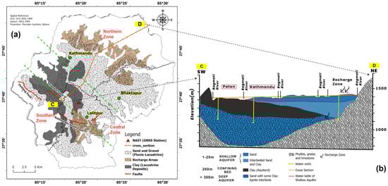
Figure 1.
(a) Modified hydrogeology of Kathmandu Valley [32]. Fault lines are represented in red line modified from Asahi [33], and Green dashed line separates the three recharge zones; South, Central and Northern zones as defined by JICA [32]. (b) Schematic geological cross-section of profile CD through Central Nepal modified from Cresswell [34].
The tectonic activity has given rise to multiple faults in the region such as Thankot Fault, Chandragiri Fault, Thimi Fault, and Patan Bhaktapur Fault. Among these, only the Thankot Fault remains tectonically active, with an observed vertical displacement rate of 1 mm/yr [33]. Given the region’s high seismic activity, these faults have the potential to be reactivated by seismic events, leading to localized ground deformation [35]. Therefore, studying subsidence in the region is essential for ensuring infrastructure resilience and enhancing disaster preparedness to effectively mitigate earthquake hazards.
2.2. Interferometric Synthetic Aperture Radar
InSAR is a powerful technique for monitoring land deformation, utilizing satellite imagery to generate displacement maps by analyzing phase differences across multiple interferograms. It offers millimeter-level accuracy and is widely employed to detect surface changes, fault movements, subsidence, and uplift caused by both natural and human-induced factors. Persistent Scatter (PS-InSAR)and small baseline subset (SBAS) are commonly used InSAR method for measuring slow deformation.
For our study, we will use the SBAS InSAR technique to study the land subsidence that uses multiple stacked master slave pairs of Sentinel-1 Satellite data. The results will be validated for consistency and accuracy using GNSS, PS-InSAR, and histogram methods. The free InSAR processing tool LiCSBAS [36] is used to download the LiCSAR products (Unwrapped interferograms), which are publicly available to download through COMET-LiCS web portal (https://comet.nerc.ac.uk/COMET-LiCS-portal/, accessed on 22 October 2024). The datasets span for 7.6 years, from Jan 2017 to July 2024. The frame IDs 085A_06253_131313 and 019D_06217_131313 were used to download both ascending and descending (Figure 2) interferograms. These interferograms cover 250 km swath at 5 m by 20 m spatial resolution, geocoded onto a 100 m grid.
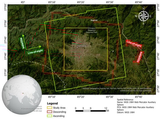
Figure 2.
Geographical location of study area. The area with white borders represents the clipped area for our study. The red and green box represents the schematic diagram of two frames 019D_06217_131313 and 085A_06253_131313 in descending and ascending orbits in COMET-LiCS Web Portal [37].
During the initial processing steps of InSAR, 849 datasets from descending orbits and 983 from ascending orbits were retained after removing initially faulty interferograms identified through a visual inspection of the png file format of each interferogram. The network of available interferometric pairs along with their temporal-baseline information of interferograms used for SBAS and PS-InSAR is shown in Figure 3.
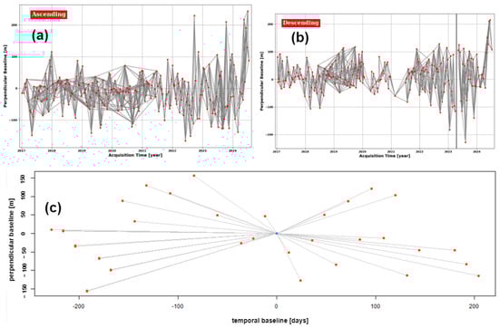
Figure 3.
Spatial and temporal baseline of InSAR analysis (a) SBAS; ascending orbits, (b) SBAS; descending orbits, and (c) PSI; ascending orbits.
The atmospheric correction was applied using GACOS external files. During loop closure and quality checks, with a coherence threshold of 0.05, 63 interferograms from the descending frame and 26 from the ascending frame were identified as faulty and excluded from further processing. The remaining interferograms were processed using the small baseline inversion approach to generate velocity results, while time-series analysis was performed using the least squares method for each pixel, further minimizing residual noise. LiCSBAS selects a stable, high-coherence location as the reference area. The same reference area is utilized in PS InSAR to ensure consistent results prior to validation between the two methods. The InSAR results are in a line-of-sight (LOS) direction and not direct vertical motion. Equation (1) is used to decompose ascending and descending LOS velocity into horizontal and vertical components [38].
where is the incidence angle, is the azimuth angle. and are the LOS deformation in ascending and descending orbit direction. and are the vertical and horizontal displacement components.
2.3. Groundwater Level Data
Groundwater levels can influence both elastic and inelastic land deformation. When the water level remains above the pre-consolidation head, only elastic deformation occurs. However, if the water level drops below the pre-consolidation head, permanent deformation takes place. A hydrological cross-section of Kathmandu Valley reveals a three-tiered aquifer system comprised of an unconfined shallow aquifer, an aquitard, and a confined aquifer (Figure 4b).
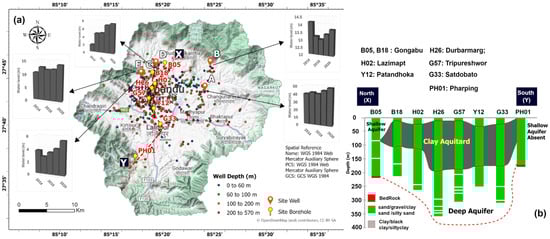
Figure 4.
(a) Distribution of wells in Kathmandu Valley. The red label represents the borehole along profile XY whose cross-section is shown in (b) The bar graph represents the water level from 2014 to 2020 of selected tubewell A, B, C, D and E. (b) Hydrogeological cross-section along spatial profile XY modified after Pandey [39].
The shallow aquifer (0–60 m), primarily utilized for household purposes, is widely distributed across the valley, while deeper wells (>60 m), mainly used for industrial purposes, are concentrated in the central basin [39]. The two shallow and confined deep aquifers are separated by a silt-rich clay layer, with varying thicknesses (5 to 200 m) [32,40,41,42]. The shallow aquifer gradually decreases in thickness from the northern valley towards the center, while the deep aquifer is thickest in the central and southern regions [41]. Spatial and temporal land-use and land-cover (LULC) analysis has revealed that Kathmandu Valley has experienced the highest increase in built-up areas in the country. Over the last 30 years (1990–2020), built-up areas have expanded by 368.06% [43], significantly reducing natural groundwater recharge zones. This urban expansion has also limited open spaces, preventing rainwater from infiltrating the soil and replenishing groundwater reserves. While monsoon rainfall recharges shallow aquifers, leading to a temporary minor rebound in land elevation but prolonged droughts, soil compaction and unregulated groundwater extraction without adequate replenishment can result in inelastic subsidence [44].
The total reported number of tube wells was 60 in 1989 [45], which increased to 218 according to a report by Metcalf and Eddy in 2000 [41]. By 2009, a KUKL report recorded 379 tube wells within the valley. Currently, 104 deep tube wells extract approximately 54 MLD (Million Liters per Day) of groundwater [16]. Understanding groundwater dynamics is essential for evaluating subsidence risks. However, historical groundwater level data are scarce. There is very limited groundwater level data available primarily gathered by independent researchers, NGOs, and government agencies in fragmented efforts. The primary sources of water well data and locations were obtained from (https://gw-nepal.com, accessed on 11 December 2024) and Smartphones4Water Nepal (https://s4w-nepal.smartphones4water.org, accessed on 17 November 2024). Additional undocumented well data were collected from independent researchers and local ward offices. Figure 4a shows the distribution of wells in Kathmandu Valley, highlighting a high concentration of deep wells in the northwestern and central regions. These areas are also highly urbanized, with a significant presence of industries, commercial and education institutional buildings. Despite gaps in water level data for many wells, five sites were selected based on their continuous and long-term data availability. Figure 4a shows the water level data for each well in February from 2014 to 2020, with the most significant decline observed in Well D, located in the northwestern part of the valley. In this study, InSAR time-series analysis will be conducted at these five sites to examine the correlation between subsidence and groundwater levels. The recent well data will also be analyzed to determine water level trends, further exploring the relationship between subsidence and groundwater depletion.
2.4. Emerging Hot Spot Analysis
Emerging hot spot analysis (EHA) is a powerful tool in ArcGIS that utilizes the Space–Time Cube (STC) to detect patterns in InSAR-derived subsidence data over a given study period [26,46,47]. The STC is a three-dimensional framework for analyzing spatial and temporal data, stored as discrete bins. In this structure, the XY plane represents spatial dimensions, while the Z-axis represents time. The STC is stored in netCDF format, organizing data in an (x, y, z, t) array, where x and y denote spatial coordinates, t represents time, and z stores attributes such as subsidence magnitude, precipitation, or slope. To analyze trends within each bin, the Mann–Kendall statistical test is applied, which evaluates the direction and statistical significance of temporal changes using z-scores and p-values. A negative z-score indicates a decreasing trend, while a positive z-score signifies an increasing trend. A low p-value suggests statistical significance. The EHA utilizes the netCDF-based STC as an input, applying Getis-Ord Gi* statistics to identify spatial and temporal patterns in subsidence data. This method assesses whether a feature is a significant hot spot (clusters of high values) or cold spot (clusters of low values) based on its neighboring bins. Figure 5 illustrates the EHA process, where individual bins with a temporal dimension along the Z-axis are combined to form a STC.
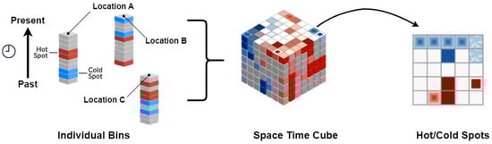
Figure 5.
Emerging hot spot analysis workflow diagram modified [48,49].
InSAR-derived displacement data were initially stored in .csv format, with latitude and longitude in the first two columns and cumulative displacement values recorded across multiple SAR acquisition dates. The dataset was transposed and pre-processed for STC formation, using mean displacement as the summary field. A 200 m spatial resolution was selected, averaging all points within each grid cell to create temporal slices preserving displacement trends. To analyze subsidence patterns, the 3D Space–Time Cube Explorer was used for visualizing individual bins and spatial trends. The generated STC served as an input for EHA, where individual time steps were examined instead of the entire cube to avoid misinterpretations from broader regional trends. For this study, eight key patterns were selected to accurately represent subsidence trends (Table 2).
Table 2.
Emergency hot analysis patterns.
2.5. Geological Composition and Land-Use Data
Land subsidence is significantly influenced by the geological composition of the study area. Groundwater exploitation, uncontrolled urban expansion, large-scale construction activities and presence of unconsolidated sediments are key factors contributing to subsidence processes in urban environments. To investigate these influences, we will overlay the InSAR-derived subsidence map with both the geological formation map and the land-use map, generated through GIS-based spatial analysis. Pandey and Kazama conducted a comprehensive hydrogeological study to map the spatial distribution of aquifer characteristics, including the thickness, transmissivity (T), hydraulic conductivity, and storage coefficient of both shallow and deep aquifers. The study involved constructing a hydrogeologic cross-section, differentiating shallow aquifers, aquitards, and deep aquifers based on sediment stratigraphy from eight boreholes along profile line XY (Figure 4b) [39]. To study a correlation between sediment thickness and subsidence, we will analyze InSAR time-series trends at these borehole sites. For a broader regional assessment, we have constructed columnar sections using additional borehole data from GWDP and JICA along profile line AB (south–north) and MN (west–east) (Figure 6a). This will allow us to examine the spatial relationship between geological formations, land-use patterns, and subsidence rates. Figure 6b illustrates the stratigraphic column along the west–east (WE) section, revealing that clay thickness is greatest in the central region, a trend also observed in the south-north (SN) cross-section (Figure 6c). The low-porosity, highly impermeable black clay layer within the aquitard zone becomes more dominant toward the center of the valley.
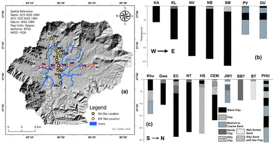
Figure 6.
(a) Hill Shed Map of study area, where blue represents the major rivers. Bagmati river is the primary drainage of valley and main outlet for water flow from valley. The sites of boreholes used to construct columnar sections of sediment lithology are shown in yellow and red circles along NS and SW direction in map. (b) The columnar section along MN. (c) Columnar section along AB.
Esri has made the global land-use map available using Sentinel-2 data at a 10 m resolution, processed through Impact Observatory’s deep learning AI land classification model. The model was trained on five billion hand-labeled Sentinel-2 pixels collected from 20,000 sites representing major global biomes. The maps are available from 2017 to 2023, classifying land cover into nine distinct categories. They are distributed under the Creative Commons Attribution (CC BY 4.0) license, requiring proper attribution. The web applications can be accessed from (https://livingatlas.arcgis.com/landcoverexplorer/, accessed on 20 January 2025). The webapp enables users to visualize global land-use cover, side-by-side comparisons across different years and animation features to observe temporal changes. For research and analysis, GeoTIFF files of the study region are available for download. This accessibility reduces computational time and resource consumption, making it a valuable tool for large-scale environmental and land-use studies.
3. Results
3.1. Land Subsidence Results
To analyze the spatial and temporal distribution of ground subsidence in the study region, ascending and descending unwrapped interferograms were downloaded from LiCSAR for the period 2017 to 2024. The interferograms were processed using LiCSBAS batch processing, incorporating external GACOS files to generate velocity maps and time-series data. The results from the ascending and descending images were decomposed using Equation (1) to derive vertical displacements (Figure 7a).
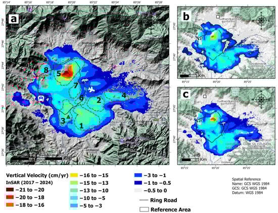
Figure 7.
(a) Vertical Velocity InSAR Map from SBAS method using LiCSBAS (2017–2024). Red dashed line denotes the eight areas selected for zonal analysis based on significant subsidence rates (b) Velocity Map in Ascending Direction (2017–2024). (c) Velocity Map in Descending Direction (2017–2024). These figures were made using Arc GIS Pro 3.4.0.
The velocity maps reveal that subsidence is unevenly distributed across the region. Significant subsidence is concentrated in the northwest region, and most of the subsidence is distributed near the Ring Road. The maximum observed subsidence is ~21 cm/year, with a vertical cumulative displacement of ~1.5 m over 91 months. Areas with mixed-use zones such as Maharajgunj, Samakhusi, Baluwatar, Lazimpat, Dhumbarahi, Sukedhara, Bishalnagar, and Lainchaur, which are densely populated and highly urbanized with the maximum number of hotels, industries, and the tallest business complexes, exhibited the highest subsidence rates. Significant subsidence was also recorded in Koteshwor, a mixed-use settlement area. Further, the old settlement areas like Patan and suburb areas like Gwarko, which also has many brick kilns, exhibited considerable subsidence. In the outskirts of the valley near the northeastern region, in the area between Bode, Duwakot, and Bhatgaon, close to the Kathmandu Model College (KMC), a significant subsidence has been observed. To study the spatial extent of subsidence, eight Regions of Interest (ROIs) were defined around areas showing significant subsidence, as indicated by dashed red lines in Figure 7a. The Zonal Statistics tool in ArcGIS Pro was used to compute statistical summaries for these ROI zones (Table 3).
Table 3.
Zonal statistics summary of subsidence of selected ROI.
Overextraction of water has resulted in formation of bull’s-eye patten formation in zone 5 of subsidence map, which also exhibits the highest subsidence rate compared to rest of the study area. Figure 8a shows the time series of vertical displacement and mean subsidence rates at borehole sites along the profile XY (Figure 4a).
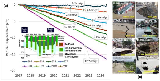
Figure 8.
(a) InSAR-derived time series and mean vertical velocity of eight borehole sites whose location is shown in Figure 4a across profile line XY, (b) columnar section of eight boreholes (c) Recent reported damages seen in various locations of our study area such as landslide, fissures, and sinkhole formation [50].
Equation (2) is used to transform the ascending LOS into vertical displacement of each borehole site. H26 and H02, located in the central region, recorded maximum subsidence rates of −13 cm/year and −17 cm/year, respectively. In contrast, boreholes PH01, B05, and B018, situated in the northern and southeastern regions where the aquitard is minimal or absent, exhibited negligible subsidence. This highlights that subsidence in the valley is primarily driven by sediment compaction, with the aquitard playing a critical role. The aquitard, composed of clay, acts as a barrier separating the shallow and confined deep aquifers and plays a significant role in driving subsidence. During monsoon season, the shallow aquifer is recharged by rainwater and nearby rivers, which experience peak water flow, resulting in an elastic rebound of land surface. This is reflected by oscillatory patterns in the time series for regions near the rivers. Figure 4a and Figure 7a elucidate that areas experiencing maximum subsidence have large number of deep tubewells that extract large amount of groundwater from deep confined aquifers. The time series of this region has liner trend dominant with minimal seasonal fluctuations, indicating that the observed extreme subsidence is mainly associated with deep groundwater pumping, where seasonal rainfall has limited influence. The impermeable black clay layer prevents rainwater from penetrating and recharging the deep aquifer, resulting in a persistent decline in water levels. This decrease in water levels is accompanied by soil compaction, further exacerbating the region’s vulnerability to subsidence.
where is the vertical displacement, is the LOS displacement, and is the incident angle.
The ArcGIS Surface Profile tool was employed to visualize the subsidence change across profile AB and MN (Figure 9). The primary objective was to analyze subsidence rates at each borehole location and assess the correlation between sediment thickness, land use, lithology and vertical subsidence.
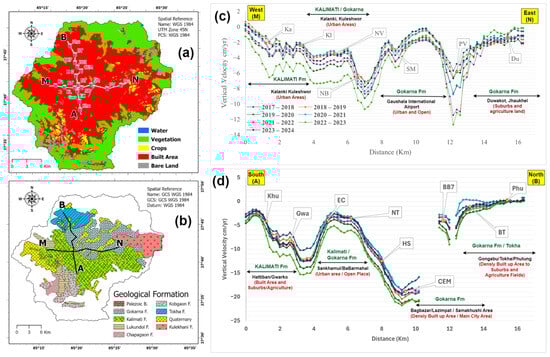
Figure 9.
(a) Sentinel 2 LULC Map from ESRI [51]. (b) Geology of Kathmandu Valley, modified from [52,53]. (c) Vertical Mean Velocity along profile line MN. (d) Vertical Mean Velocity across profile AB. The labeled borehole site’s location and columnar section are shown in Figure 6.
Figure 9c,d illustrate the undulating pattern of subsidence along both the north-south (NS) and east–west (EW) spatial profiles. A comparison of the subsidence profile with the land classification map (Figure 9a) and geological map (Figure 9b) reveals that the highest subsidence occurs within the Kalimati Formation and Gokarna Formation, predominantly in regions with a high density of urban development. Both formations consist of highly unconsolidated sediments, including sand, silt, clay, and gravel [28]. The Kalimati Formation is primarily composed of black clay, silt, and fine sand, indicative of a low-energy depositional environment associated with the prehistoric Kathmandu Paleo-Lake. The substantial clay content of low permeability in this region impedes the penetration of rainwater in deep confined aquifers, thereby intensifying subsidence. The expansion of built-up areas in such region that absorbs minimal rainwater increases surface imperviousness, leading to heightened waterlogging increased runoff, and elevated flood risk. The high pumping of groundwater in the Gokarna Formation, consisting mainly of fine-grained sand and silt layers, reduces pore water pressure, which exacerbates the risk of subsidence in these areas. A bivariate analysis of the vertical velocity (Figure 9c,d) and columnar section (Figure 6b,c) reveals that regions with the greatest thickness of sediment deposits, predominantly black clay, experience the highest subsidence. The borehole sites HS and NT along the AB profile across NS, characterized by a high clay content, exhibit the highest subsidence rates. Similarly, the borehole sites NV, NB, and SM along the MN profile across EW, which are also predominantly composed of black clay, experience significant subsidence rates.
3.2. Cross-Validation
The InSAR deformation rate is measured relative to a local reference point, requiring quantitative assessment for accurate interpretation. Our study area has only one available GPS station (NAST), which includes a 26-month data gap (11 December 2019–27 November 2021), potentially impacting the reliability of subsidence rate analysis. Given the study region’s size (~310 sq. km) and uneven deformation rates, a single GPS station is insufficient for validating InSAR-derived surface motion. To ensure accuracy, we used PS-InSAR, differential analysis of ascending and descending deformation rates, and GPS data for the cross-validation of LOS results. This multi-validation approach enhances reliability at GPS station locations, high-density PS areas, and regions covered by both ascending and descending orbits.
3.2.1. GNSS and Histogram Difference Technique
The GPS data for the NAST station were obtained from the Nevada Geodetic Laboratory (NGL) (http://geodesy.unr.edu/, accessed on 5 October 2024) based on IGS14 as the reference frame, covering the same period as the InSAR time series [54]. While GPS measures deformation in NS, EW, and UD directions, InSAR records displacement in the satellite’s LOS direction , requiring conversion to vertical displacement using Equation (2) [55]. As shown in Figure 10a, both ascending and descending InSAR displacement trends indicate an increasing subsidence rate, aligning with GPS observations.
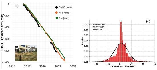
Figure 10.
(a) Time-series comparisons of GPS and ascending and descending cumulative displacement with precipitation from 2017 to 2024. (b) GPS station (NAST) used in this study [56]. (c) Mean velocity difference of ascending and descending orbit histogram.
At the GPS site (85.328, 27.657), the subsidence rate estimated by InSAR is −112 ± 29 mm/yr, compared to −125.92 mm/yr from GPS. This discrepancy may result from a 26-month GPS data gap (11 December 2019–27 November 2021), differences in data acquisition frequency (InSAR: 12 days, GPS: daily), spatial resolution, satellite look angle, and seasonal variations. A differential analysis of ascending and descending deformation rates provides an alternative consistency check, especially when no GNSS station or PS-InSAR data is available [57,58]. Figure 10c presents a histogram (bin size = 80) and a normal curve fit for deformation rate differences, with most values ranging between +40 and −40 mm/yr. The mean (2.68 mm/yr) and median (2.77 mm/yr) indicate minimal difference, confirming good consistency between results. A skewness value of 0.09 suggests a nearly symmetric distribution, while a kurtosis of 2.26 (<3) reflects a platykurtic distribution, indicating fewer extreme values. Minor discrepancies may be due to elevation differences, incidence angles, heading directions, or temporal variations.
3.2.2. PS-InSAR Method
The PS-InSAR technique [59] utilizes permanent scatterers (PS), primarily man-made structures, to analyze stable reflection signals for time-series generation using the SNAP-StaMPS workflow. This technique is highly effective for monitoring urban land deformation, achieving millimeter-level accuracy with a minimum of 20 images [60]. For this study, 31 Sentinel-1A SLC images in ascending orbit (IW mode, VV polarization) were acquired from September 2023 to November 2024 via ASF. The image from 23 March 2024 was selected as the master image, with the remaining images co-registered with master image to generate interferograms. The details of the datasets are given in Table A1. The SNAP toolbox was used for interferogram generation, followed by snap2stamps [61] to automate processing for StaMPS [62]. The final LOS displacement was derived from Matlab (StaMPS) using seven processing steps. As shown in Figure 11a, the PS-InSAR analysis also identifies the same regions, outlined by blue-bordered rectangle, experiencing significant subsidence consistent with SBAS analysis (Figure 7a). The findings from these two methods demonstrate a strong agreement.
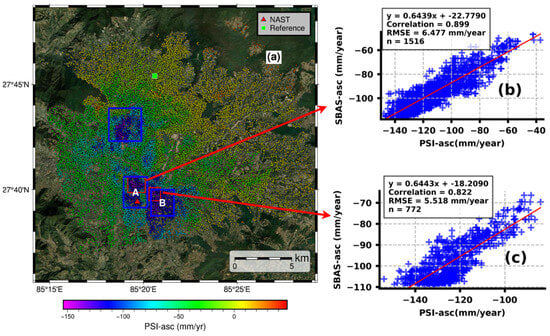
Figure 11.
(a) PS-InSAR deformation map from ascending track. The three large rectangles outlined in red shows region with highest subsidence. The small rectangle with red outline is common overlapping area between SBAS and PSI pixel used for correlation analysis. (b) Scatter plot between LiCSBAS results and PS-InSAR velocity of region inside label A. (c) Scatter plot between LiCSBAS and PS-InSAR velocity of region inside box label B.
However, subtle differences in subsidence rates may arise due to variations in processing methods, temporal gaps, foreshortening, layover, shadow effects, and different orbital direction and incidence angle. The two regions shown by red rectangle in Figure 11a labeled A and B were selected to compare results for an accuracy assessment of SBAS and InSAR methods. The two regions were chosen based on their extensive coverage and high pixel density, ensuring greater precision in the comparison. Region A, consisting of 1516-pixel points, demonstrated a correlation coefficient of 0.899 and a root mean square error (RMSE) of 6.477 mm/year, indicating strong agreement. Similarly, Region B, which contains 671 PS points, exhibited a correlation of 0.822 with an RMSE of 5.518 mm/year, reflecting a slightly lower but still substantial consistency in subsidence measurements (Figure 11b,c). These results confirm a strong correlation between PS-InSAR and SBAS, validating the subsidence patterns. Since this study primarily focuses on SBAS-InSAR subsidence analysis, PS-InSAR was only analyzed for 31 ascending orbit images (2023–2024) to check the accuracy of SBAS results. Further improvements in correlation and RMSE may be achieved by increasing PS-InSAR temporal resolution to match the SBAS time range.
3.3. Temporal and Spatial Changes of Emerging Hot Spots (2017–2024)
The EHA tool was applied to examine the spatiotemporal patterns of InSAR-derived subsidence trends. This analysis integrates two key statistical methods: the Getis–Ord Gi* statistic and the Mann–Kendall trend test. Figure 12a presents the EHSA results, highlighting subsidence patterns from 2017 to 2024.
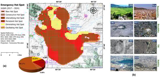
Figure 12.
(a) Emerging hot spot analysis of InSAR vertical deformation rates (this was prepared using ArcGIS Pro). (b) Expansion of urban areas across various areas of Kathmandu Valley [63,64].
The intensifying hot spots are the most prevalent pattern, accounting for 56.17% of all detected hot spots. The intensifying hot spot areas are primarily concentrated in the Kathmandu and Lalitpur districts, where InSAR analysis indicates subsidence rates ranging from 0.5 cm/year to 15 cm/year. Persistent hot spots, covering 22.84% of the valley, are aligned along the Ring Road and concentrated in high-population-density areas, including Balaju (west), Madhyapur Thimi (east), and Lalitpur (south). The clusters of persistent hot spots in Gongabu and Madhyapur Thimi are interconnected along the Ring Road corridor, suggesting a relationship between subsidence and urban development. The hot spot clusters bifurcate near Madhyapur Thimi (east) and Gongabu (northwest), with branches extending north and south from Madhyapur Thimi, while those from Gongabu extend northward toward Pharping and westward toward Balaju. In southern Lalitpur, a cluster of persistent hot spots suggest ongoing subsidence, likely driven by intensive groundwater extraction in areas with a high concentration of hotels and a dense population. Meanwhile, diminishing hot spots occupy 15.87% of the study area, primarily located east of the Tribhuvan International Airport (TIA) up to Duwakot and northwest from Baneshwor to Tarkeshwor, indicating that subsidence has slowed over time. The diminishing hot spot cluster in the northwest coincides with the highest subsidence rates observed in the InSAR-derived velocity map, indicating a temporal shift in subsidence intensity. This deceleration may be attributed to the increased water supply from the Melamchi Water Supply Project (MWSP), completed in 2021, as well as from the Bagmati River. Since its implementation, the proportion of groundwater extraction in total water production has decreased from 43% in 2021 to nearly 8% in 2024 [16]. However, further analysis is necessary to gain a deeper understanding of the underlying mechanisms driving this trend.
3.4. Groundwater Status
The rapid urbanization and population growth have led to an exponential increase in water demand within KV, rising from an estimated 214.6 in 2001 to 506 MLD in 2024. During the same period, the population grew from 1.5 million to approximately 3 million. However, a limited government initiative was undertaken to enhance surface water supply, placing significant stress on groundwater resources. To address this growing water crisis, the MWSP aimed at delivering 170 MLD of water through a 26.4 km diversion tunnel, which was initiated in 1998 and completed in 2021. Following the completion of MWSP in 2021, water production has improved significantly. However, a deficit of 40% remains relative to total demand. Figure 13c shows a steady increase in water supply each year, but without timely interventions, climate change and prolonged droughts are likely to exacerbate water shortages in the future, increasing the deficit percentage further.
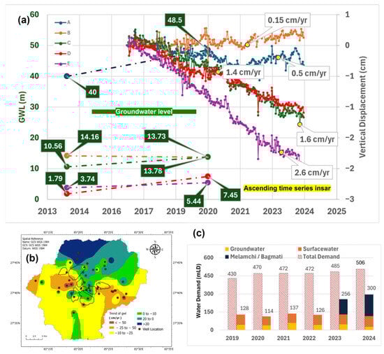
Figure 13.
(a) Water level data of five well locations from 2012 to 2014 (left) and InSAR time series from 2017 to 2024 (right). (b) IDW interpolation of groundwater level rate of change of well from S4W from 2018 to 2022 across 46 wells; black boundary represents the zonal ROI based on Figure 7a; (c) KUKL water supply statistics (2029–2024).
The line of sight (LOS) deformation from ascending orbit was transformed into vertical displacement for five selected well monitored by GWRDP between 2014 and 2020 using Equation (2) (Figure 13a). These sites were selected based on data frequency and time span. Among the observed wells, Well E exhibited the highest subsidence, followed by Wells C and D, all located in highly urbanized and industrialized areas. In contrast, Well A showed minimal subsidence, while Well B exhibited a slight uplift of 0.15 cm/year. These wells are situated on the outskirts of the valley, where shallow bedrock and minimal sediment thickness contribute to greater resistance against subsidence. Since these wells primarily extract water from shallow aquifers, which are naturally replenished by rainfall and nearby rivers, their water level data may not sufficiently correlate with InSAR-derived subsidence trends, particularly if subsidence is driven by deeper aquifer depletion. This limitation results in a weak correlation between observed water level fluctuations and ground deformation. Currently, data from deep boreholes is scarce, restricting comprehensive analysis. Future studies incorporating water level records from deeper tube wells will be essential for improving the understanding of groundwater extraction’s role in subsidence and enhancing the accuracy of InSAR-based assessments.
The continuous subsidence trend with a steep negative slope, without significant seasonal oscillation, suggests that deep aquifer extraction, which lacks direct rainfall recharge, is the primary driver of land deformation in the study area. Despite limited historical groundwater data, recent records from S4W-Nepal (S4W-Nepal) were obtained from (https://smartphones4water.org, accessed on 12 September 2024). S4W-Nepal, a non-profit research organization founded in 2017, leverages mobile technology to collect hydro-meteorological data in Nepal by mobilizing young researchers to enhance water management. To ensure consistency, a filter was applied to retain only wells with at least 70% data coverage, identifying a period where the maximum number of wells had continuous observations. The results showed that 44 wells met this criterion between 2018 and 2022, the highest number available. Inverse Distance Weighting (IDW) interpolation was applied based on the linear trend of groundwater levels, allowing for the visualization of spatial patterns across the region, as illustrated in Figure 13b. The groundwater level is declining at a rate of up to 0.7 m/year in areas with high density of deep boreholes (Figure 4a). These areas are also experiencing accelerated subsidence, as indicated by InSAR results, highlighting that groundwater extraction from confined deep aquifer is primary driver of subsidence in KV.
4. Discussion
Vigilant monitoring of land subsidence constitutes a critical endeavor to forestall future geohazards and avert irreversible consequences. In high-density urban areas with extensive built environments, subsidence control is both technically challenging and economically prohibitive if early warning signals are ignored, leading to substantial financial and infrastructural losses. The situation is particularly alarming in seismically vulnerable cities like Kathmandu, where active fault lines lie in proximity. This study employs LiCSBAS to process InSAR data for a comprehensive analysis of subsidence in the study region. For the first time, we integrate LiCSBAS results into a Space–Time Cube framework and utilize emerging hot spot analysis (EHA) for spatiotemporal assessment, identifying significant subsidence hot spots and cold spots. The study reveals that the subsidence trend is decreasing in area, which shows a maximum subsidence rate, probably due to a reduction in groundwater extraction by KUKL after the MWSP became operational. Also, the northwestern region with high number of industries, hotels, and commercial buildings and maximum concentration of deep tubewell over Gokarna Formation experiences subsidence rates reaching up to ~21 cm per year.
Despite the severity of subsidence in Kathmandu Valley, Kathmandu has been conspicuously absent from global subsidence rankings. Bagheri-Gavkosh [65], in their analysis of 290 metropolitan cities based on the published literature, categorized subsidence into five groups, with the highest rate (20.1–39 cm/year) occurring in 3.1% of cases and the second highest (11.31–20 cm/year) in 9.8% of cases. Their study highlights eastern China, the Marand Plain in Iran, the Texas Gulf Coast, northern Jakarta, and the Mexico City Metropolitan Area as having the most severe subsidence. Kathmandu, however, is absent from these assessments. Similarly, a global land subsidence study by Davydzenka [12] synthesizing 221 individual publications and open-source data places Nepal’s maximum recorded subsidence at merely 3.8 cm/year, positioning it near the bottom of global rankings. Another study by Tzampoglou [13] examined subsidence rates across various cities and found values ranging from 0.1 cm/year to a maximum of ~35 cm/year in Mexico City. The study attributes approximately 40% of observed subsidence to urbanization, particularly in Mexico City, Beijing, Semarang, and Tehran, with additional contributions from industrial, agricultural, and anthropogenic impacts. Kathmandu remains excluded from these analyses as well. This research aims to bridge that gap by providing robust evidence that positions Kathmandu Valley among the world’s most subsidence-prone urban areas. Figure 14a delineates areas affected by subsidence based on rate and cumulative displacement.
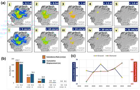
Figure 14.
(a) The first and second row images illustrate regions affected by varying subsidence rates and total displacement, as detected by InSAR from 2017 to 2024. (b) The bar diagram quantifies the total area impacted by subsidence, categorizing affected regions based on the color-coded classifications in (a). (c) The trend graph depicts the total water demand and groundwater extraction (measured in million liters per day, MLD) from 2019 to 2024.
A histogram (Figure 14b) visualization categorizes total affected areas into five classes, revealing that ~174.7 square kilometers exhibit subsidence below 5 cm/year, while ~155.4 square kilometers have undergone cumulative displacement of ~20 cm between 2017 and 2024, signifying a dire scenario. Less than 3 square kilometers, predominantly in the northeastern region, experience subsidence exceeding 15 cm/year, while 3.3 square kilometers have suffered vertical displacement exceeding 1.6 m in just eight years. To contextualize these findings, Bangkok has subsided 1.25 m over 113 years (2–3 cm/year), New Orleans by 1.13 m over the same period (6 cm/year), Shanghai by 2–3 m since 1920 (5 mm/year), and Tianjin by 3–5 m (3–30 mm/year). Jakarta has recorded a subsidence of 2.5–4 m from 1970 to 2020 (25–30 cm/year), while Tehran has subsided 3–5 m (25 cm/year). Ho Chi Minh City has recorded a 1–2 m subsidence over 50 years (20–25 mm/year) [13]. While these cities required decades to centuries to accrue over 2 m of subsidence, Kathmandu’s pace positions it among the world’s swiftest-subsiding urban centers. Our findings indicate that deep aquifer depletion is a primary driver of land subsidence in Kathmandu Valley. This conclusion aligns with the findings of Huang [24], who also identified groundwater extraction as a significant factor contributing to subsidence in the region. Shallow aquifers are primarily recharged by rainwater or nearby streams; however, this process contributes minimally to the replenishment of deep aquifers. The expansion of built-up areas into peripheral zones, encroaching upon open spaces near mountainous regions, is likely to exacerbate the subsidence. Several studies on the interaction of shallow aquifer and nearby rivers have confirmed the hydraulic connectivity between the two systems. Malla [66] analyzed stable water isotopes in the Bagmati and Bishnumati Rivers, revealing significant mixing with nearby wells. Prajapati [67] found that 12% of wells had higher water levels than adjacent streams in pre-monsoon conditions, while 69% exhibited higher levels in post-monsoon periods. Bajracharya [68] quantified stream–aquifer interactions and confirmed significant hydrological exchanges near river channels. The time-series analysis from this study reveals oscillations in areas near shallow boreholes, suggesting elastic land rebound following seasonal recharge. While research on the recharge mechanisms of deep aquifers in our study area remains limited, Martinelli’s [69] study in Emilia-Romagna, Italy, identified land subsidence resulting from the overexploitation of deep aquifers through isotopic analysis. A significant study on the deep aquifers of Kathmandu Valley (KV) by Shakya [70] revealed that recharge primarily occurs via lateral flow from the base of surrounding mountains, augmented by the infiltration of high-frequency rainfall over prolonged periods. Therefore, additional research is essential to further elucidate the recharge dynamics of deep aquifers in KV.
Shrestha [71] in his study about the recharge rate in the aquifer of KV determined that infiltration rates are more influenced by land use than soil texture, with cultivated land exhibiting higher infiltration due to root permeability. The rapid expansion of impervious built-up areas, particularly in former agricultural zones, has significantly reduced natural recharge zones, exacerbating groundwater depletion and intensifying subsidence. Similar correlations between groundwater extraction, sediment consolidation, and subsidence have been documented in Mexico City, Jakarta, and Tianjin [13].
KUKL reports that while water demand in KV has risen by ~17% from 2019 to 2024, groundwater extraction has declined by 39.4% (Figure 14c). The additional water supply from MWSP and the Bagmati River has significantly reduced dependency on groundwater. Thapa [72] projected a land rebound of up to ~5 m if MWSP reaches full operational capacity, a prediction corroborated by Shrestha [73], who developed the first land subsidence model using SHETRAN and MODFLOW. A similar trend was observed in Houston, Texas, where a study of 95 GNSS stations between 2005 and 2012 recorded a slight land rebound following enforced groundwater withdrawal regulations [1]. The MWSP and Bagmati Water Supply Project have demonstrated a positive impact in curbing subsidence. Migration trends indicate that major cities in Nepal’s Terai region are also experiencing rapid urbanization, leading to increasing water scarcity same as KV. Reports have emerged regarding declining tubewell water levels. Luitel [74] investigated subsidence in Pokhara (another major metropolitan city) using Sentinel-1 SAR data and found an average rate of 16 cm/year, indicating that subsidence is not confined to the Terai but also affects hilly regions, with potential intensification in near future. Therefore, more research is crucial to assess subsidence in urban regions across the country, in order to mitigate potential geohazards and promote sustainable water and land management strategies. Our results are accessible online via a web application (https://ktmsub.alwaysdata.net, accessed on 11 February 2025), developed by the authors to provide readers with interactive access to our findings.
5. Conclusions
This study used LiCSBAS to process InSAR data from 2017 to 2024, enabling a spatiotemporal analysis of land subsidence in the study area. The InSAR data were integrated with the EHA tool to assess changes in subsidence patterns following the implementation of the Melamchi Water Supply Project (MWSP) in 2021. Our findings indicate that significant subsidence is occurring across the region, with rates reaching up to ~21 cm/year (2017–2024) and cumulative displacement exceeding ~1.5 m. The most affected areas are densely populated urban centers with high concentrations of industries, hotels, educational institutions, and commercial buildings. The results align with previous research, reaffirming that excessive groundwater extraction from deep aquifers is the primary driver of subsidence. Similar patterns have been observed in other cities experiencing rapid groundwater depletion, including Mexico City, Jakarta, and Houston, Texas [13].
The most impacted locations include Bagbazar, Lazimpat, Lainchaur, and Balaju (Kathmandu), Madhyapur Thimi and Lokanthali (Bhaktapur), and Gwarko and Patan (Lalitpur), with subsidence extending into peripheral areas such as Gothatar, Bode, Imadol, Satungal, and Dhapasi Tokha in the northeastern region. Previous studies predicted that subsidence rates would decline with the increased availability of surface water from MWSP and Bagmati River. Our EHA analysis has shown decline in subsidence intensity in previously high-risk zones. The EHA analysis of InSAR data shows a decline in subsidence in parts of the northwestern KV. However, MWSP has been operational for only three years and has faced temporary disruptions due to flooding. To ascertain this relationship with greater precision, extended temporal data will be essential in the future, alongside comprehensive ground-based measurements. This study has demonstrated the efficacy of three validation techniques that can facilitate accuracy assessments for various methodologies in the absence of GNSS data.
While current mitigation strategies have shown promising results, water demand continues to rise, leaving 40% of total demand unmet. Policy interventions must prioritize mandatory borehole registration, groundwater monitoring, and restrictions on new infrastructure in vulnerable zones. Decentralized urban planning, infrastructure upgrades, rainwater harvesting, and the establishment of artificial recharge zones should be integral to future strategies aimed at preventing further subsidence. This research provides critical insights for urban planners and policymakers, offering data-driven recommendations to mitigate economic and infrastructural losses caused by land subsidence. By guiding long-term urban resilience strategies, these findings can help ensure sustainable development and safeguard the stability of rapidly expanding urban centers.
Author Contributions
Conceptualization, S.R. and G.W.; methodology, S.R.; software, S.R.; validation, S.R.; formal analysis, S.R.; investigation, S.R.; data curation, S.R.; writing—original draft preparation, S.R.; writing—review and editing, S.R. and G.W.; visualization, S.R.; supervision, G.W. All authors have read and agreed to the published version of the manuscript.
Funding
This research received no external funding.
Data Availability Statement
Sentinel data: SBAS InSAR time series was formed using unwrapped interferograms obtained from https://comet.nerc.ac.uk/COMET-LiCS-portal/, accessed on 22 October 2024 using frame 019D_06217_131313 and 085A_06253_131313 for descending and ascending orbits from 2017 to 2024. PS-InSAR analysis was performed using data obtained from the NASA’s Alaska Satellite Facility Distributed Active Archive Center (ASF DAAC) from 2023 to 2024 (https://search.asf.alaska.edu/, accessed on 22 May 2023). LULC maps were downloaded from https://livingatlas.arcgis.com/landcoverexplorer (accessed on 25 December 2024). Metrological Data: The precipitation data were acquired from the Department of Hydrology and Meteorology, Nepal, upon request (https://www.dhm.gov.np/, accessed on 15 December 2024). GNSS Data: The GNSS data for station “NAST” were obtained from https://geodesy.unr.edu/, accessed 11 December 2024. Water-well data: The water-well data were obtained from the Groundwater Development Resource Project (https://gw-nepal.com/, accessed 20 December 2024) and S4W (https://s4w-nepal.smartphones4water.org/, accessed 11 December 2024).
Acknowledgments
LiCSAR contains modified Copernicus Sentinel data (2017–2024) analyzed by the Centre for the Observation and Modelling of Earthquakes, Volcanoes and Tectonics (COMET). LiCSAR uses JASMIN, the UK’s collaborative data analysis environment (http://jasmin.ac.uk) (accessed on 22 October 2024). We are immensely grateful to the editor and anonymous reviewers for their comments on the manuscript. I would like to thank Jack Thomson for a detailed review of the manuscript.
Conflicts of Interest
The authors declare no conflicts of interest.
Abbreviations
The following abbreviations are used in this manuscript:
| EHA | Emergency Hot Spot Analysis |
| GACOS | Generic Atmospheric Correction Online Service for InSAR |
| MWSP | Melamchi Water Supply Project |
| KV | Kathmandu Valley |
| DHM | Department of Hydrology and Meteorology |
| KUKLLOS | Kathmandu Upatyaka Khanepani LimitedLine of Sight |
Appendix A
Table A1.
Sentinel 1A Dataset Information for PS-InSAR Processing.
Table A1.
Sentinel 1A Dataset Information for PS-InSAR Processing.
| Orbit | Path | Period | Frame | Azimuth | Master | Total | Incidence | Sub Swath | |
|---|---|---|---|---|---|---|---|---|---|
| Asc | 85 | September 2023 | November 2024 | 88 | 350.92° | 28 March 2024 | 31 | 39.46° | IW2 |
References
- Kearns, T.J.; Wang, G.; Bao, Y.; Jiang, J.; Lee, D. Current Land Subsidence and Groundwater Level Changes in the Houston Metropolitan Area (2005–2012). J. Surv. Eng. 2015, 141, 05015002. [Google Scholar]
- Ge, L.; Ng, A.H.M.; Du, Z.; Chen, H.Y.; Li, X. Integrated Space Geodesy for Mapping Land Deformation over Choushui River Fluvial Plain, Taiwan. Int. J. Remote Sens. 2017, 38, 6319–6345. [Google Scholar] [CrossRef]
- Gao, M.; Gong, H.; Chen, B.; Li, X.; Zhou, C.; Shi, M.; Si, Y.; Chen, Z.; Duan, G. Regional Land Subsidence Analysis in Eastern Beijing Plain by InSAR Time Series and Wavelet Transforms. Remote Sens. 2018, 10, 365. [Google Scholar] [CrossRef]
- Yin, J.; Yu, D.; Wilby, R. Modelling the Impact of Land Subsidence on Urban Pluvial Flooding: A Case Study of Downtown Shanghai, China. Sci. Total Environ. 2016, 544, 744–753. [Google Scholar] [CrossRef]
- Wang, G.; Greuter, A.; Petersen, C.M.; Turco, M.J. Houston GNSS Network for Subsidence and Faulting Monitoring: Data Analysis Methods and Products. J. Surv. Eng. 2022, 148, 04022008. [Google Scholar]
- Li, Z.; Chen, Q.; Xue, Y.; Qiu, D.; Chen, H.; Kong, F.; Liu, Q. Numerical Investigation of Processes, Features, and Control of Land Subsidence Caused by Groundwater Extraction and Coal Mining: A Case Study from Eastern China. Environ. Earth Sci. 2023, 82, 82. [Google Scholar]
- Meng, D.; Chen, B.; Gong, H.; Zhang, S.; Ma, R.; Zhou, C.; Lei, K.; Xu, L.; Wang, X. Land Subsidence and Rebound Response to Groundwater Recovery in the Beijing Plain: A New Hydrological Perspective. J. Hydrol. Reg. Stud. 2025, 57, 102127. [Google Scholar]
- Tang, W.; Zhao, X.; Motagh, M.; Bi, G.; Li, J.; Chen, M.; Chen, H.; Liao, M. Land Subsidence and Rebound in the Taiyuan Basin, Northern China, in the Context of Inter-Basin Water Transfer and Groundwater Management. Remote Sens. Environ. 2022, 269, 112792. [Google Scholar]
- Wang, K.; Wang, G.; Bao, Y.; Su, G.; Wang, Y.; Shen, Q.; Zhang, Y.; Wang, H. Preventing Subsidence Reoccurrence in Tianjin: New Preconsolidation Head and Safe Pumping Buffer. Groundwater 2024, 62, 778–794. [Google Scholar]
- Zhang, W.; Zhang, T.; Fu, Z.; Ai, P.; Yao, G.; Qi, J. Emerging Spatio-Temporal Hot Spot Analysis of Beijing Subsidence Trend Detection Based on PS-InSAR. Int. Arch. Photogramm. Remote Sens. Spat. Inf. Sci. 2024, 48, 861–866. [Google Scholar]
- Lees, M.; Knight, R. Quantification of Record-Breaking Subsidence in California’s San Joaquin Valley. Commun. Earth Environ. 2024, 5, 677. [Google Scholar] [CrossRef]
- Davydzenka, T.; Tahmasebi, P.; Shokri, N. Unveiling the Global Extent of Land Subsidence: The Sinking Crisis. Geophys. Res. Lett. 2024, 51, e2023GL104497. [Google Scholar] [CrossRef]
- Tzampoglou, P.; Ilia, I.; Karalis, K.; Tsangaratos, P.; Zhao, X.; Chen, W. Selected Worldwide Cases of Land Subsidence Due to Groundwater Withdrawal. Water 2023, 15, 1094. [Google Scholar] [CrossRef]
- Mushrooming Concrete Houses in Kathmandu: Harms Are Visible, but a Solution Is Nowhere in Sight | Aζ South Asia. Available online: https://architexturez.net/pst/az-cf-219351-1618362841 (accessed on 14 March 2025).
- Census Nepal. 2021. Available online: https://censusnepal.cbs.gov.np/Home/Index/EN (accessed on 19 August 2024).
- Kathmandu Upatyaka Khanepani Limited (KUKL)—Water. Available online: https://kathmanduwater.org/ (accessed on 19 August 2024).
- Dahal, A.; Khanal, R.; Mishra, B.K. Identification of Critical Location for Enhancing Groundwater Recharge in Kathmandu Valley, Nepal. Groundw. Sustain. Dev. 2019, 9, 100253. [Google Scholar] [CrossRef]
- United Nations Development Programme, Bureau for Crisis Prevention and Recovery. Reducing Disaster Risk: A Challenge for Development: A Global Report. Disaster and Crisis Management; United Nations: New York, NY, USA, 2004; p. 143.
- Acharya, P.; Sharma, K.; Acharya, I.P. Seismic Liquefaction Risk Assessment of Critical Facilities in Kathmandu Valley, Nepal. GeoHazards 2021, 2, 153–171. [Google Scholar] [CrossRef]
- Bhattarai, R.; Alifu, H.; Maitiniyazi, A.; Kondoh, A. Detection of Land Subsidence in Kathmandu Valley, Nepal, Using DInSAR Technique. Land 2017, 6, 39. [Google Scholar] [CrossRef]
- Krishnan, P.V.S.; Kim, D.; Jung, J. Land Subsidence Monitoring in the Kathmandu Basin, Before and After MW 7.8 Gorkha Earthquake, Nepal by Sbas-Dinsar Technique. In Proceedings of the IGARSS 2018–2018 IEEE International Geoscience and Remote Sensing Symposium, Valencia, Spain, 22–27 July 2018; IEEE: New York, NY, USA, 2018; pp. 525–528. [Google Scholar]
- Kumahara, Y.; Chamlagain, D.; Upreti, B.N. Geomorphic Features of Active Faults around the Kathmandu Valley, Nepal, and No Evidence of Surface Rupture Associated with the 2015 Gorkha Earthquake along the Faults. Earth Planets Space 2016, 68, 1–8. [Google Scholar] [CrossRef]
- Bhandari, S. Detecting Surface Displacement in Kathmandu Valley with Persistent Scatterer Interferometry. J. Geoinform. Nepal 2022, 21, 23–29. [Google Scholar] [CrossRef]
- Huang, J.; Sinclair, H.; Pokhrel, P.; Watson, C.S. Rapid Subsidence in the Kathmandu Valley Recorded Using Sentinel-1 InSAR. Int. J. Remote Sens. 2024, 45, 1–20. [Google Scholar] [CrossRef]
- Privileges Documentation Esri Developer. Documentation; Esri Developer: Redlands, CA, USA, 2025. [Google Scholar]
- Khan, S.D.; Faiz, M.I.; Gadea, O.C.A.; Ahmad, L. Study of Land Subsidence by Radar Interferometry and Hot Spot Analysis Techniques in the Peshawar Basin, Pakistan. Egypt. J. Remote Sens. Space Sci. 2023, 26, 173–184. [Google Scholar] [CrossRef]
- Sakai, H. Stratigraphic Division and Sedimentary Facies of the Kathmandu Basin Group, Central Nepal. J. Nepal Geol. Soc. 2001, 25, 19–32. [Google Scholar]
- Stocklin, J.; Bhattarai, K.D. Geology of Kathmandu Area and Central Mahabharat Range, Nepal Himalaya. HMG/UNDP Mineral Exploration Project; Technical Report; HMG/UNDP Mineral Exploration Project: Kathmandu, Nepal, 1977; 128p. [Google Scholar]
- Paudel, M.R.; Sakai, H. Stratigraphy and Depositional Environments of Basin-Fill Sediments in Southern Kathmandu Valley, Central Nepal. Bull. Dep. Geol. 2008, 11, 61–70. [Google Scholar]
- Yoshida, M. Neogene to Quartenery Lacustrine Sediments In The Kathmandu Valley, Nepal. J. Nepal Geol. Soc. Spec. Issue 1984, 4, 73–100. [Google Scholar]
- Pandey, V.P.; Chapagain, S.K.; Kazama, F. Evaluation of Groundwater Environment of Kathmandu Valley. Environ. Earth Sci. 2010, 60, 1329–1342. [Google Scholar] [CrossRef]
- JICA (Japan International Cooperation Agency). Groundwater Management Project in the Kathmandu Valley, Final; Japan International Cooperation Agency: Kathmandu, Nepal, 1990. [Google Scholar]
- Asahi, K. Thankot Active Fault in the Kathmandu Valley, Nepal Himalaya. J. Nepal Geol. Soc. 2003, 28, 1–8. [Google Scholar]
- Cresswell, R.G.; Bauld, J.; Jacobson, G.; Khadka, M.S.; Jha, M.G.; Shrestha, M.P.; Regmi, S. A First Estimate of Ground Water Ages for the Deep Aquifer of the Kathmandu Basin, Nepal, Using the Radioisotope Chlorine-36. Groundwater 2001, 39, 449–457. [Google Scholar]
- Ghimire, S.; Dwivedi, S.K.; Acharya, K.K. Pattern of Ground Deformation in Kathmandu Valley during 2015 Gorkha Earthquake, Central Nepal. In Proceedings of the AGU Fall Meeting Abstracts; American Geophysical Union: Washington, DC, USA, 2016; Volume 2016, p. S33D-2859. [Google Scholar]
- Morishita, Y.; Lazecky, M.; Wright, T.J.; Weiss, J.R.; Elliott, J.R.; Hooper, A. LiCSBAS: An Open-Source InSAR Time Series Analysis Package Integrated with the LiCSAR Automated Sentinel-1 InSAR Processor. Remote Sens. 2020, 12, 424. [Google Scholar]
- Wright, T.J.; Gonzalez, P.J.; Walters, R.J.; Hatton, E.L.; Spaans, K.; Hooper, A.J. LiCSAR: Tools for Automated Generation of Sentinel-1 Frame Interferograms. In Proceedings of the AGU Fall Meeting Abstracts; American Geophysical Union: Washington, DC, USA, 2016; Volume 2016, p. G23A-1037. [Google Scholar]
- Manzo, M.; Ricciardi, G.P.; Casu, F.; Ventura, G.; Zeni, G.; Borgström, S.; Berardino, P.; Del Gaudio, C.; Lanari, R. Surface Deformation Analysis in the Ischia Island (Italy) Based on Spaceborne Radar Interferometry. J. Volcanol. Geotherm. Res. 2006, 151, 399–416. [Google Scholar] [CrossRef]
- Pandey, V.P.; Kazama, F. Hydrogeologic Characteristics of Groundwater Aquifers in Kathmandu Valley, Nepal. Environ. Earth Sci. 2011, 62, 1723–1732. [Google Scholar] [CrossRef]
- Gurung, J.K.; Ishiga, H.; Khadka, M.S.; Shrestha, N.R. The Geochemical Study of Fluvio-Lacustrine Aquifers in the Kathmandu Basin (Nepal) and the Implications for the Mobilization of Arsenic. Environ. Geol. 2007, 52, 503–517. [Google Scholar]
- Metcalf & Eddy, Inc.; CEMAT Consultants Ltd. Urban Water Supply Reforms in the Kathmandu Valley; Asian Development Bank: Manila, Philippines, 2000. [Google Scholar]
- Shakya, B.M.; Nakamura, T.; Kamei, T.; Shrestha, S.D.; Nishida, K. Seasonal Groundwater Quality Status and Nitrogen Contamination in the Shallow Aquifer System of the Kathmandu Valley, Nepal. Water 2019, 11, 2184. [Google Scholar] [CrossRef]
- Devkota, P.; Dhakal, S.; Shrestha, S.; Shrestha, U.B. Land Use Land Cover Changes in the Major Cities of Nepal from 1990 to 2020. Environ. Sustain. Indic. 2023, 17, 100227. [Google Scholar] [CrossRef]
- Galloway, D.L.; Jones, D.R.; Ingebritsen, S.E. Land Subsidence in the United States; Geological Survey (USGS): Reston, VA, USA, 1999; Volume 1182, ISBN 0607926961.
- GWRDB (Groundwater Resource Development Board). Vulnerability Study in Budhanilkantha and Sorrounding Area Kathmandu Nepal; Groundwater Resource Development Board: Kathmandu, Nepal, 2009. [Google Scholar]
- Khan, S.D.; Gadea, O.C.A.; Tello Alvarado, A.; Tirmizi, O.A. Surface Deformation Analysis of the Houston Area Using Time Series Interferometry and Emerging Hot Spot Analysis. Remote Sens. 2022, 14, 3831. [Google Scholar] [CrossRef]
- Mohamadi, B.; Balz, T.; Younes, A. Towards a PS-InSAR Based Prediction Model for Building Collapse: Spatiotemporal Patterns of Vertical Surface Motion in Collapsed Building Areas—Case Study of Alexandria, Egypt. Remote Sens. 2020, 12, 3307. [Google Scholar] [CrossRef]
- Emerging Hot Spot Analysis (Space Time Pattern Mining)—ArcGIS Pro Documentation. Available online: https://pro.arcgis.com/en/pro-app/latest/tool-reference/space-time-pattern-mining/emerginghotspots.htm (accessed on 13 December 2024).
- Space-Time Cubes: Stack Time Like Lego—GIS Geography. Available online: https://gisgeography.com/space-time-cubes (accessed on 15 December 2024).
- Ekantipur. Available online: https://ekantipur.com (accessed on 21 December 2024).
- Karra, K.; Kontgis, C.; Statman-Weil, Z.; Mazzariello, J.C.; Mathis, M.; Brumby, S.P. Global Land Use/Land Cover with Sentinel 2 and Deep Learning. In Proceedings of the 2021 IEEE International Geoscience and Remote Sensing Symposium IGARSS, Brussels, Belgium, 11–16 July 2021; IEEE: New York, NY, USA, 2021; pp. 4704–4707. [Google Scholar]
- Shallow Aquifer Mapping of Kathmandu Valley. Available online: https://www.academia.edu/27155659/Shallow_Aquifer_Mapping_of_Kathmandu_Valley (accessed on 20 August 2024).
- Gilder, C.E.L.; Pokhrel, R.M.; Vardanega, P.J.; De Luca, F.; De Risi, R.; Werner, M.J.; Asimaki, D.; Maskey, P.N.; Sextos, A. The SAFER Geodatabase for the Kathmandu Valley: Geotechnical and Geological Variability. Earthq. Spectra 2020, 36, 1549–1569. [Google Scholar] [CrossRef]
- Blewitt, G.; Hammond, W.; Kreemer, C. Harnessing the GPS Data Explosion for Interdisciplinary Science. Eos 2018, 99, e2020943118. [Google Scholar]
- Fuhrmann, T.; Garthwaite, M.C. Resolving Three-Dimensional Surface Motion with InSAR: Constraints from Multi-Geometry Data Fusion. Remote Sens. 2019, 11, 241. [Google Scholar] [CrossRef]
- UNAVCO. Available online: https://www.unavco.org/instrumentation/networks/status/other/overview/NAST (accessed on 22 January 2025).
- Radman, A.; Akhoondzadeh, M.; Hosseiny, B. Integrating InSAR and Deep-Learning for Modeling and Predicting Subsidence over the Adjacent Area of Lake Urmia, Iran. GIScience Remote Sens. 2021, 58, 1413–1433. [Google Scholar]
- Wang, Y.; Guo, Y.; Hu, S.; Li, Y.; Wang, J.; Liu, X.; Wang, L. Ground Deformation Analysis Using InSAR and Backpropagation Prediction with Influencing Factors in Erhai Region, China. Sustainability 2019, 11, 2853. [Google Scholar] [CrossRef]
- Ferretti, A.; Prati, C.; Rocca, F. Nonlinear Subsidence Rate Estimation Using Permanent Scatterers in Differential SAR Interferometry. IEEE Trans. Geosci. Remote Sens. 2000, 38, 2202–2212. [Google Scholar]
- Ciampalini, A.; Raspini, F.; Lagomarsino, D.; Catani, F.; Casagli, N. Landslide Susceptibility Map Refinement Using PSInSAR Data. Remote Sens. Environ. 2016, 184, 302–315. [Google Scholar] [CrossRef]
- Delgado Blasco, J.M.; Ziemer, J.; Foumelis, M.; Dubois, C. SNAP2StaMPS v2: Increasing Features and Supported Sensors in the Open Source SNAP2StaMPS Processing Scheme; Zenodo: Stordalen Mire, Sweden, 2025. [Google Scholar] [CrossRef]
- Hooper, A.; Spaans, K.; Bekaert, D.; Cuenca, M.C.; Arıkan, M.; Oyen, A. StaMPS/MTI Manual. Delft Institute of Earth Observation and Space Systems; Delft University of Technology, Kluyverweg: Delft, The Netherlands, 2010; Volume 1, p. 2629. [Google Scholar]
- ChangeKathmandu. Available online: https://x.com/ChangeKathmandu (accessed on 19 December 2024).
- ICIMOD. Available online: https://geoapps.icimod.org/ktmbeforeafter (accessed on 10 January 2025).
- Bagheri-Gavkosh, M.; Hosseini, S.M.; Ataie-Ashtiani, B.; Sohani, Y.; Ebrahimian, H.; Morovat, F.; Ashrafi, S. Land Subsidence: A Global Challenge. Sci. Total Environ. 2021, 778, 146193. [Google Scholar] [CrossRef] [PubMed]
- Malla, R.; Shrestha, S.; Chapagain, S.K.; Shakya, M.; Nakamura, T.; Malla, R.; Shrestha, S.; Chapagain, S.K.; Shakya, M.; Nakamura, T. Physico-Chemical and Oxygen-Hydrogen Isotopic Assessment of Bagmati and Bishnumati Rivers and the Shallow Groundwater along the River Corridors in Kathmandu Valley, Nepal. J. Water Resour. Prot. 2015, 7, 1435–1448. [Google Scholar] [CrossRef]
- Prajapati, R.; Overkamp, N.N.; Moesker, N.; Happee, K.; van Bentem, R.; Danegulu, A.; Manandhar, B.; Devkota, N.; Thapa, A.B.; Upadhyay, S.; et al. Streams, Sewage, and Shallow Groundwater: Stream-Aquifer Interactions in the Kathmandu Valley, Nepal. Sustain. Water Resour. Manag. 2021, 7, 1–18. [Google Scholar]
- Bajracharya, R.; Nakamura, T.; Shakya, B.M.; Nishida, K.; Das Shrestha, S.; Tamrakar, N.K. Identification of River Water and Groundwater Interaction at Central Part of the Kathmandu Valley, Nepal Using Stable Isotope Tracers. Int. J. Adv. Sci. Tech. Res. 2018, 8, 29–41. [Google Scholar] [CrossRef]
- Martinelli, G.; Chahoud, A.; Dadomo, A.; Fava, A. Isotopic Features of Emilia-Romagna Region (North Italy) Groundwaters: Environmental and Climatological Implications. J. Hydrol. 2014, 519, 1928–1938. [Google Scholar] [CrossRef]
- Shakya, B.M.; Nakamura, T.; Das Shrestha, S.; Nishida, K. Identifying the Deep Groundwater Recharge Processes in an Intermountain Basin Using the Hydrogeochemical and Water Isotope Characteristics. Hydrol. Res. 2019, 50, 1216–1229. [Google Scholar] [CrossRef]
- Shrestha, G.; Shakya, B.M.; Shrestha, M.B.; Khadka, U.R. Water Infiltration Rate in the Kathmandu Valley of Nepal amidst Present Urbanization and Land-Use Change. H2Open J. 2023, 6, 1–14. [Google Scholar] [CrossRef]
- Thapa, B.R.; Ishidaira, H.; Gusyev, M.; Pandey, V.P.; Udmale, P.; Hayashi, M.; Shakya, N.M. Implications of the Melamchi Water Supply Project for the Kathmandu Valley Groundwater System. Water Policy 2019, 21, 120–137. [Google Scholar] [CrossRef]
- Shrestha, P.K.; Shakya, N.M.; Pandey, V.P.; Birkinshaw, S.J.; Shrestha, S. Model-Based Estimation of Land Subsidence in Kathmandu Valley, Nepal. Geomat. Nat. Hazards Risk 2017, 8, 974–996. [Google Scholar] [CrossRef]
- Luitel, S.; Ghimire, S.; Chaulagain, S.; Sah, S.; Khatri Thapa, D.; Lamichhane, S.; Civil, B.E. Assessment of Land Subsidence Pattern in Pokhara Valley Using Sentinel-1 InSAR Processing. J. Eng. Technol. Plan. 2024, 5, 27–37. [Google Scholar]
Disclaimer/Publisher’s Note: The statements, opinions and data contained in all publications are solely those of the individual author(s) and contributor(s) and not of MDPI and/or the editor(s). MDPI and/or the editor(s) disclaim responsibility for any injury to people or property resulting from any ideas, methods, instructions or products referred to in the content. |
© 2025 by the authors. Licensee MDPI, Basel, Switzerland. This article is an open access article distributed under the terms and conditions of the Creative Commons Attribution (CC BY) license (https://creativecommons.org/licenses/by/4.0/).