1. Introduction
Landslides are a common hazard in open-pit mines, frequently occurring in shallow overburden or highly weathered rock slopes. As mining depth increases and slope angles change, the need for enhanced analysis of slope landslide susceptibility becomes more critical. Common methods include landslide susceptibility assessment based on physical principles and data-driven approaches. Among these, physical-principle-based landslide susceptibility assessment primarily relies on numerical simulations of slope instability processes, with commonly used methods including the limit equilibrium method [
1,
2] and the finite element method [
3,
4]. Data-driven landslide sensitivity analysis is commonly used to study regional landslide disasters. It primarily employs machine learning, neural networks, and other techniques to analyze existing landslide cases and predict future disasters. The landslide susceptibility map generated through machine learning-based analysis is crucial for predicting regional landslide risk [
5]. A key research direction in this field is optimizing intelligent algorithms to improve model accuracy, including Logistic Regression (LR) [
6,
7], Support Vector Machines (SVMs) [
8,
9], Convolutional Neural Networks (CNNs) [
10,
11], and Artificial Neural Networks (ANNs) [
12,
13], as well as integrating different algorithms for further improvements [
14]. Examples include Bagging [
15,
16], MultiBoost [
17,
18], and Adaboost [
15,
19]. The second approach involves improving data quality, including both the accuracy of the data and the balance between landslide and non-landslide samples (positive and negative samples) [
20,
21]. The third involves selecting accurate and relevant landslide factors [
22,
23] to enhance the model’s representation of real-world events. The fourth involves compiling a comprehensive and effective landslide inventory. As a crucial data form for landslide sensitivity analysis, the landslide inventory reflects the spatial distribution of landslides [
24]. It is typically compiled through geological surveys, UAV scanning, and satellite image interpretation, and processed using GIS software [
25].
Although the aforementioned research improves the model’s fit and prediction accuracy for landslide events, the ‘black box’ nature of machine learning algorithms presents significant challenges in interpreting results, particularly for complex, nonlinear geological disasters like landslides. The interaction of factors like topography, engineering geology, ecological conditions, and human activities makes it challenging to identify the primary sliding factors, thereby restricting the practical use of this method in engineering applications.
The emergence of interpretable machine learning algorithms (SHAP, LIME) has made the internal operations of machine learning models more ‘transparent’ [
26,
27,
28]. SHAP values are used for both local and global interpretations of machine learning models. Locally, SHAP values explain predictions for individual instances, while globally, they reveal the overall importance of each feature across the dataset. This dual capability makes SHAP a powerful tool for model interpretation. Previous landslide sensitivity studies have primarily focused on large-scale landslide prediction, offering guidance for regional geological disaster prevention; they focus, for example, on both mountains [
29] and watersheds [
30]. This study applies landslide sensitivity analysis to open-pit mine slopes, combining it with interpretable machine learning techniques to predict landslide-prone areas and analyze key sliding factors. This approach aims to provide clear targets for slope prevention and control, reduce ineffective protection measures, and enhance the scientific basis and rationality of governance.
2. Study Area and Data Preparation
2.1. Study Area
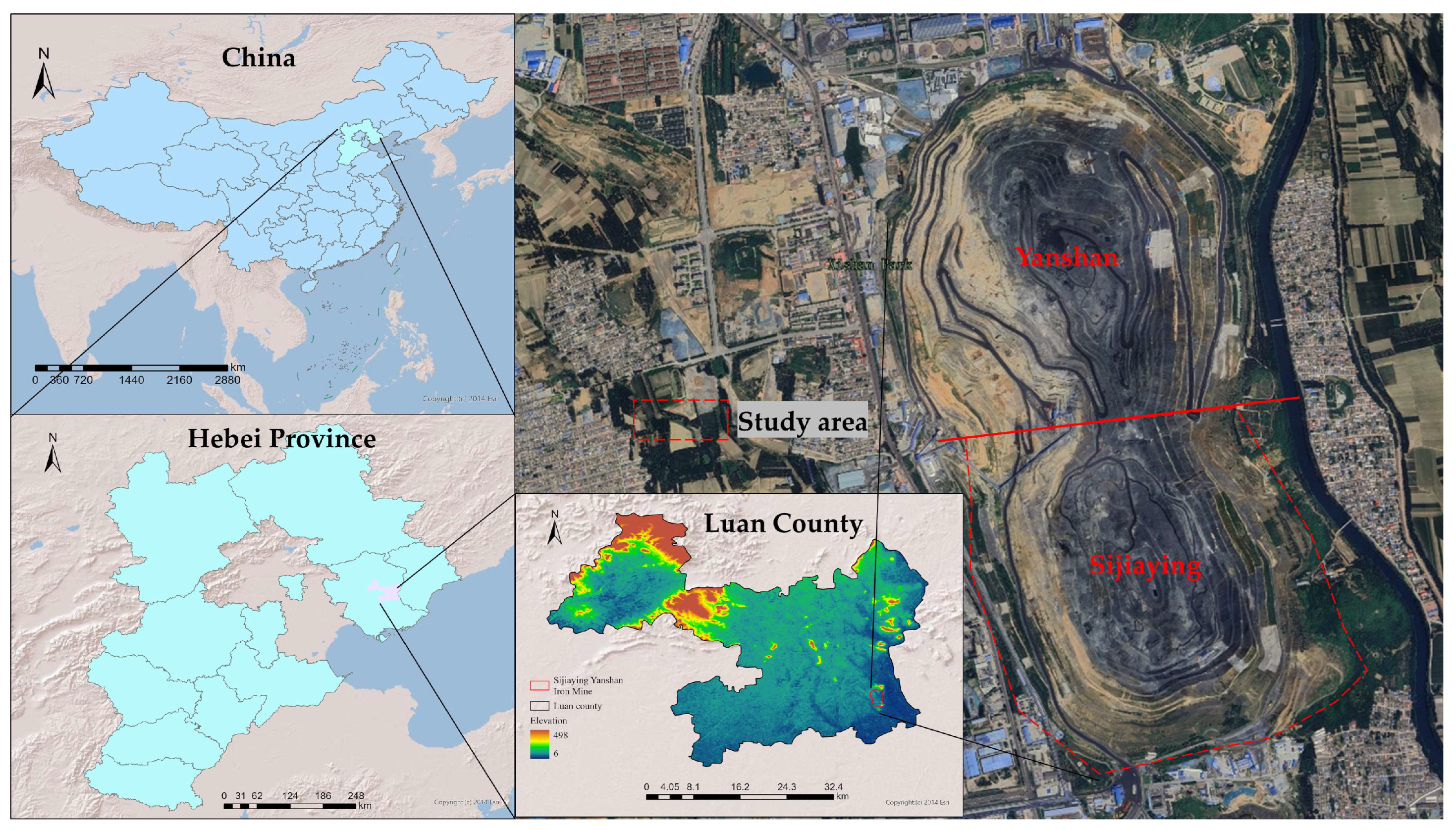
The Sijiaying Iron Mine is situated in the Yanshan Mountains, around 20 to 30 km from Tangshan City, in Hebei Province, China. The open-pit strike direction is nearly north–south (
Figure 1). The area north of the N18 exploration line is the Yanshan Iron Mine, while the area to the south is the Sijiaying Iron Mine. The central coordinates of the Sijiaying Iron Mine are 118°45′08″ E and 39°40′42″ N. The stope measures approximately 1315 m in length (north–south) and 1248 m in width (east–west), covering a total area of about 1749 km
2. The stope’s highest elevation is 85 m, and its deepest mining level reached −250 m as of 2023.
The Sijiaying iron ore deposit strikes roughly north–south and dips to the west. The western part of the stope is the hanging wall of the ore body, composed primarily of Quaternary soil, dolomite, and quartz sandstone, with the rock layers and slope dipping in the opposite direction. The eastern part of the stope is the footwall of the ore body, predominantly composed of biotite granulite with varying degrees of weathering, with the rock strata and slope dipping in the same direction. A north–south river flows 300 m to the east of the stope. The western side of the stope has been mined to the ore body’s boundary, while the eastern side remains the primary production area.
2.2. Data Preparation
2.2.1. Factors Influencing Landslide Susceptibility
Landslides are complex, systematic phenomena resulting from the interplay of multiple factors. Both predisposing and triggering factors exist. Predisposing factors refer to long-term conditions or processes that gradually reduce slope stability. These factors do not directly cause landslides but weaken slope stability, making it more susceptible to triggering factors. Triggering factors are those that abruptly alter slope stability within a short period, directly causing landslides. These factors are typically sudden and short-lived. In the study of open-pit mine landslides, predisposing factors are classified into topography, geomorphology, and geological hydrology, while triggering factors are categorized into ecological environment and mining engineering. The selection of specific influencing factors within each category varies depending on data collection methods and research objectives, with no standardized approach [
31].
This study identified 12 factors influencing landslides, chosen based on the specific characteristics of open-pit metal mine slopes. Terrain factors include height, slope [
32], and profile curvature [
33], which describe the slope body and shape. Geological and hydrological factors include lithology [
34], rock texture [
35], rock structure [
36], distance from faults, and distance from rivers [
37]. For example, lithology offers a thorough representation of the mechanical strength of the geological formation. Rock texture and rock structure reflect the micro- and macro-structural composition of the geological body. Distance from faults indicates the impact of slope rock mass structure on stability, while distance from rivers reflects the influence of hydrogeological factors on the mine slope. Ecological environment factors include surface displacement change rate [
38] and rainfall erosivity [
39,
40], which are key environmental indicators. Mining engineering factors include the peak particle vibration velocity from blasting [
41] and the distance to the road [
42]. The design of production blasting and transportation roads is the most direct factor influencing mine slope stability. The landslide locations of open-pit mine slopes were determined based on field geological surveys and disaster reports (
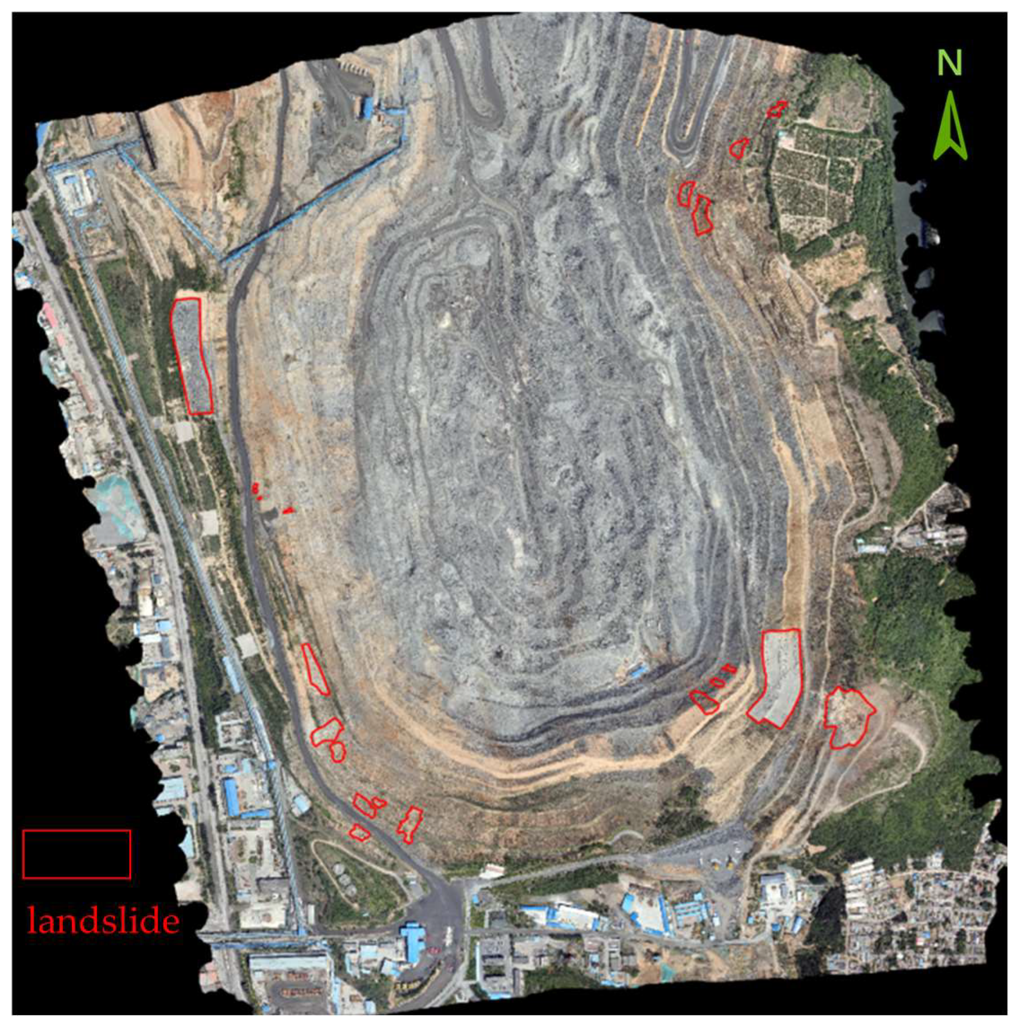
Figure 2). All landslides on the mining area slopes are shallow and small-scale. Landslides on the southwest and northeast slopes are scattered. Landslides on the northwest and southeast slopes cover a larger area. Currently, protective and reinforcement measures are implemented. The surface vector map of the landslide area was generated using ArcGIS Pro 3.0.2. The sources of the data are presented in
Table 1.
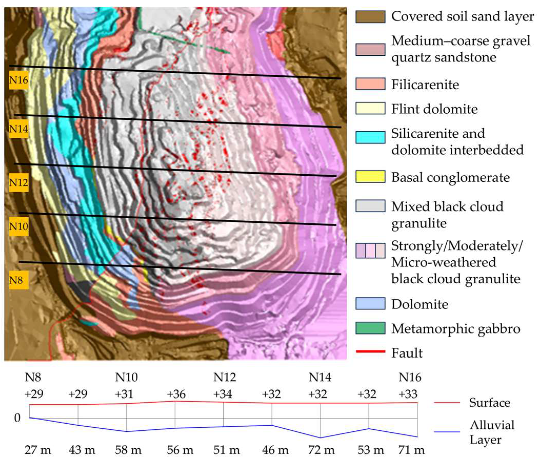
Slope height, slope, and profile curvature were derived using ArcGIS Pro 3.0.2 and Saga GIS 9.2.0, based on the DEM generated from UAV oblique photogrammetry data. Lithology, rock texture, and rock structure were mapped using ArcGIS Pro 3.0.2, based on geological data from the mine and field survey results, with corresponding attributes assigned to different geological planes. A soil sand layer is present at the −40 m to 36 m level on the west side of the Sijiaying mining area (
Figure 3). According to the Unified Soil Classification System (USCS), the layer includes SW (well-graded sands), ML (rock flour), CL (silty clays), and GC (gravelly sands). The thinnest soil layer measures 27 m and is located along the N8 exploration line. The thickest soil layer measures 72 m and is located along the N14 exploration line. Overall, the overburden is thicker on the north side than on the south side. The shallow part of the south side primarily consists of CL (silty clays) and GC (gravelly sands). The east side consists mainly of a rocky slope.
Distances to faults, rivers, and roads were computed using ArcGIS Pro 3.0.2 by plotting line vectors for each feature and then performing Euclidean distance calculations. The peak particle vibration velocity from blasting was calculated using the Sadovsky formula (Equation (1)).
In this context, V represents the peak particle vibration velocity, Q refers to the maximum charge per blast (Q = 358 kg based on the daily blasting design), K is a coefficient influenced by factors such as the blasting location, topography, and geology (K = 50), α denotes the attenuation coefficient of blasting seismic waves with increasing distance (α = 1.3), and R represents the distance between the blasting point and the measurement point. The blasting point is located along the circular line vector defined by the daily production blasting locations, and the distance to the blasting point is calculated using ArcGIS Pro 3.0.2’s Euclidean distance method.
The surface displacement change rate was obtained using the SBAS-InSAR method with Sentinel-1 data from July 2019 to July 2021. Rainfall erosivity is derived from the existing literature data [
43]. As the mining area is small and localized, rainfall data are treated as a uniform value without discrimination. Historical landslide data are represented as surface vectors.
2.2.2. Study Unit
In slope landslide sensitivity analysis, the research unit is typically either a grid unit or a slope unit [
44]. A grid unit consists of a regular square grid, with the grid size adjustable to control data accuracy. For irregular boundaries, increasing mesh accuracy may be required to simulate the boundary, but this also increases computational complexity and reduces efficiency. Slope units are advantageous for slope-related problems, as landslide evolution is driven by slopes, making them better suited to reflect the relationships between geological, topographic, and environmental boundaries. Additionally, slope units based on watershed and gully line divisions serve as the evaluation unit [
45], preserving the geological environment’s integrity within the unit, while comprehensively reflecting the influence of various factors, resulting in more realistic evaluation outcomes. Therefore, this study divides the stope slope using slope units.
2.2.3. Slope Landslide Characteristic Data Coding
ArcGIS Pro 3.0.2 was used to convert all data into vectors, followed by surface extraction based on the divided slope units, resulting in a total of 1403 data samples from 1403 slope units.
The research data include both numerical and categorical characteristics. Numerical characteristics include slope height, slope gradient, profile curvature, distance from fault, distance from river, maximum particle vibration velocity from blasting, distance from road, surface displacement change rate, and a unique value for rainfall erosivity. Categorical features include lithology, rock texture, and rock structure, which were encoded using LabelEncoder.
3. Methods
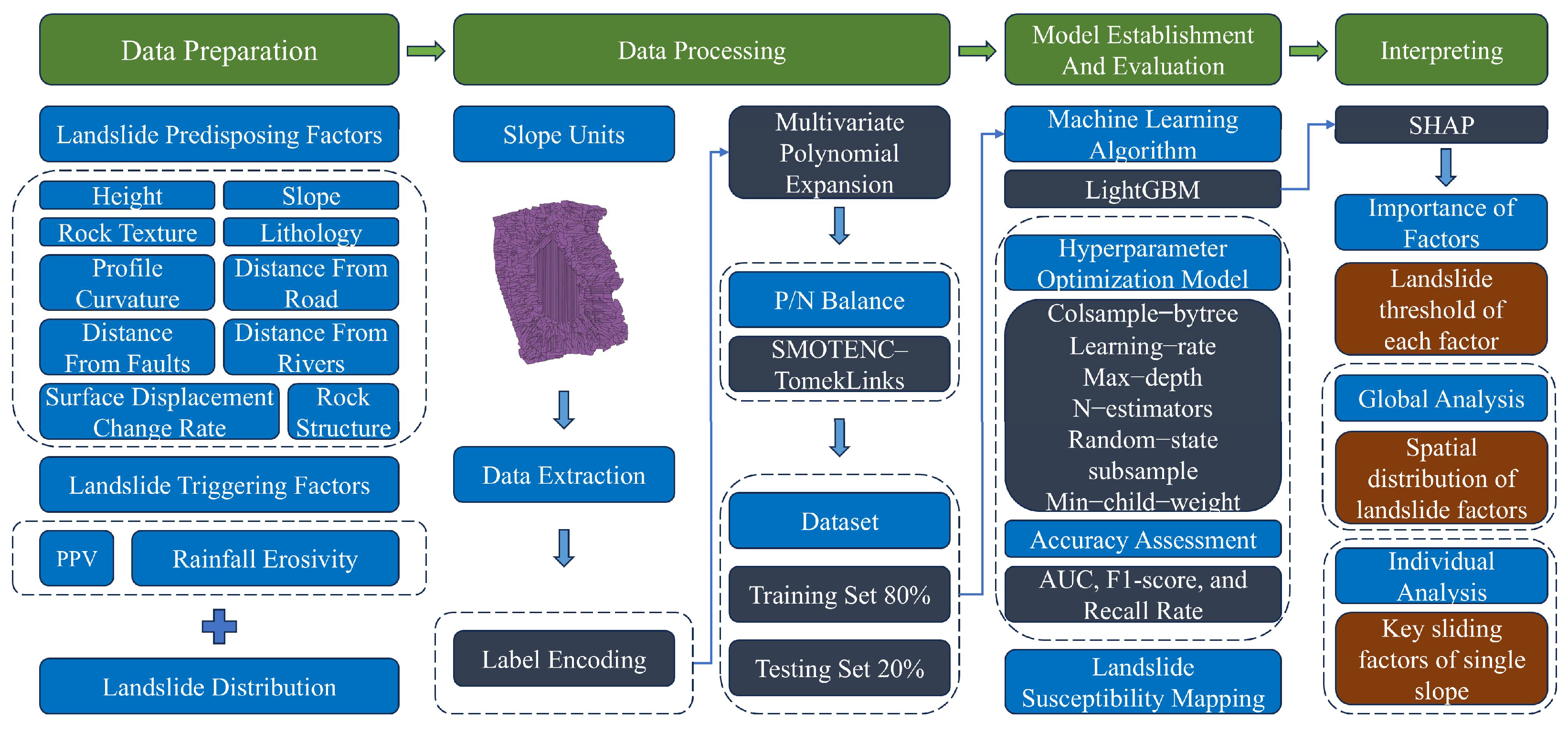
In this study, after collecting the necessary data, the data were extracted and encoded into slope units, followed by a statistical analysis of their spatial distribution. To further develop a scientific landslide sensitivity model, multivariate polynomial expansion of the data was performed to form a landslide coupling slip factor. Meanwhile, SMOTENC–TomekLinks resampling was employed to balance the positive and negative sample data. Subsequently, the dataset was divided into training and test sets, and the LightGBM algorithm was employed to construct the landslide sensitivity model. The algorithm parameters were optimized using hyperparameters, and model accuracy was evaluated using the AUC, F1-score, and recall rate. The AUC (area under the curve) [
46,
47,
48] measures model performance across all possible classification thresholds by computing the area under the ROC curve. A higher AUC value, closer to 1, indicates better classification performance. Recall [
49] measures the proportion of correctly predicted positive samples, highlighting the model’s ability to identify positive instances. The F1-score [
50], the harmonic mean of precision and recall, provides a comprehensive evaluation of classification models, particularly for imbalanced datasets. Finally, model interpretation was conducted using the SHAP algorithm. The SHAP algorithm, based on the Shapley value concept in game theory, assigns importance values to each model feature to explain the prediction process. It is characterized by model independence, local accuracy, and consistency. The SHAP algorithm can be used to determine the importance ranking of slip factors. Based on the Shapley value, the slip threshold for each factor was analyzed, and both global and individual analyses of the mine slope were conducted. Additionally, the spatial distribution of key slip factors and the diagnosis of key slip factors for individual slopes were completed. The complete technical flowchart is shown in
Figure 4.
3.1. Landslide Susceptibility Model
Data-driven landslide sensitivity analysis typically includes the frequency ratio method, the information method, and machine learning approaches. The frequency ratio method [
51] calculates the ratio between the landslide area and the landslide impact factor, using statistical techniques to express their relationship. The information method [
52] is also a statistical approach but differs from the frequency ratio method as it is based on information theory [
53]. The information value is determined by computing the logarithm of the ratio between the probabilities of landslide occurrence and non-occurrence across different classification intervals of each influencing factor, thereby reflecting the degree of correlation. Unlike the previous two statistical methods, machine learning techniques can handle high-dimensional, nonlinear, and complex data relationships, automatically identifying and learning patterns within the data while achieving high predictive accuracy. They more effectively capture the underlying patterns of landslide occurrence [
54].
LightGBM (Light Gradient Boosting Machine), developed by Microsoft [
55,
56], integrates the GBDT (Gradient Boosting Decision Tree) algorithm with advanced techniques such as GOSS (Gradient-based One-Side Sampling) and EFB (Exclusive Feature Bundling) [
57]. The algorithm was developed as a fast and efficient data science tool, characterized by low memory consumption, high accuracy, and the capability to handle parallel processing and large-scale data.
A key innovation of LightGBM is its use of a leaf-wise (best-first) growth strategy, in contrast to the depth-wise (level-wise) strategy used in traditional gradient boosting algorithms like XGBoost [
58]. This approach enables LightGBM to build trees more efficiently by prioritizing the most promising nodes, resulting in faster training times and more efficient use of computational resources.
In our experiments, we utilized LightGBM’s capabilities to build predictive models that effectively handled the complexities of our dataset. We optimized LightGBM’s hyperparameters, including the number of leaves, learning rate, and minimum data per leaf, to achieve optimal performance for our specific problem.
3.2. Multivariate Polynomial Expansion
Landslides occur due to the interaction of various factors, rather than being caused by a single determinant. They are a complex, nonlinear phenomenon. To better model the landslide problem, polynomial expansion is applied to construct the coupling characteristics.
In linear regression, polynomial expansion is a common technique used to improve the model’s fitting capability by adding more features and higher-order polynomial terms. Polynomial expansion transforms a sample vector x with n features into a vector with k features, where k represents any polynomial of n. For instance, with a quadratic polynomial expansion, the sample vector [x1, x2] is transformed into a new feature vector containing the original features and cross terms, such as [x1, x2, x12, x22, x1x2]. These new features capture richer combinations and nonlinear relationships, thereby enhancing the model’s fitting ability [
59].
After polynomial expansion, a linear regression model can be used to fit the transformed data, with the fitting error serving as a metric to evaluate model performance. Typically, as the polynomial degree increases, the model’s fitting error decreases; however, this can lead to overfitting, resulting in poor performance on new data. Therefore, when using polynomial expansion, it is crucial to balance fitting ability with generalization, employing techniques like regularization to prevent overfitting.
Polynomial expansion is carried out using the PolynomialFeatures class from the Python (3.11.0) Scikit-learn framework. This class transforms the original feature matrix x into a new matrix containing polynomial features. During conversion, PolynomialFeatures allows specification of the polynomial degree, which defines the highest degree of the expansion. In this instance, the highest degree is set to 2. PolynomialFeatures expands the original feature matrix x to include all linear, quadratic, and cross terms. The resulting feature matrix contains 90 factors, including single, self-coupling, and mutual-coupling terms.
3.3. Positive and Negative Sample Balance
Data imbalance refers to a substantial difference in the number of samples across various categories in a dataset. This often results in the model being biased toward the majority class during training, neglecting the minority class [
60,
61]. The experimental dataset contains 1276 positive samples (non-landslide) and 127 negative samples (landslide). The ratio of positive to negative samples is roughly 10:1, reflecting a typical data imbalance problem.
The SMOTE algorithm is an oversampling method that generates new synthetic instances of the minority class to balance the dataset [
62]. Unlike simple random oversampling, SMOTE generates new samples through interpolation rather than duplicating existing ones. Specifically, for each sample in the minority class, the SMOTE algorithm randomly selects one of its K-nearest neighbors and generates a new sample by selecting a point along the line connecting them.
Tomek Links is a down-sampling technique used for data cleaning. It is primarily applied to address class imbalance in classification problems [
63,
64]. It reduces the sample size by identifying and removing specific sample pairs. The goal is to create a decision space that more effectively separates the minority and majority classes.
Tomek Links is commonly combined with other sampling methods, particularly SMOTE, to form an effective strategy for addressing imbalanced datasets [
65]. First, SMOTE is employed to augment the quantity of minority instances. It creates synthetic instances by interpolating between existing minority samples, thereby facilitating a more balanced class distribution. However, SMOTE has the potential to create synthetic samples close to the boundary separating the majority and minority classes, which may obscure the decision boundary of the classifier. Subsequently, Tomek Links is utilized to eliminate overlapping instances. After SMOTE generates new samples, Tomek Links removes overlapping samples from boundary areas, clarifying the class boundaries.
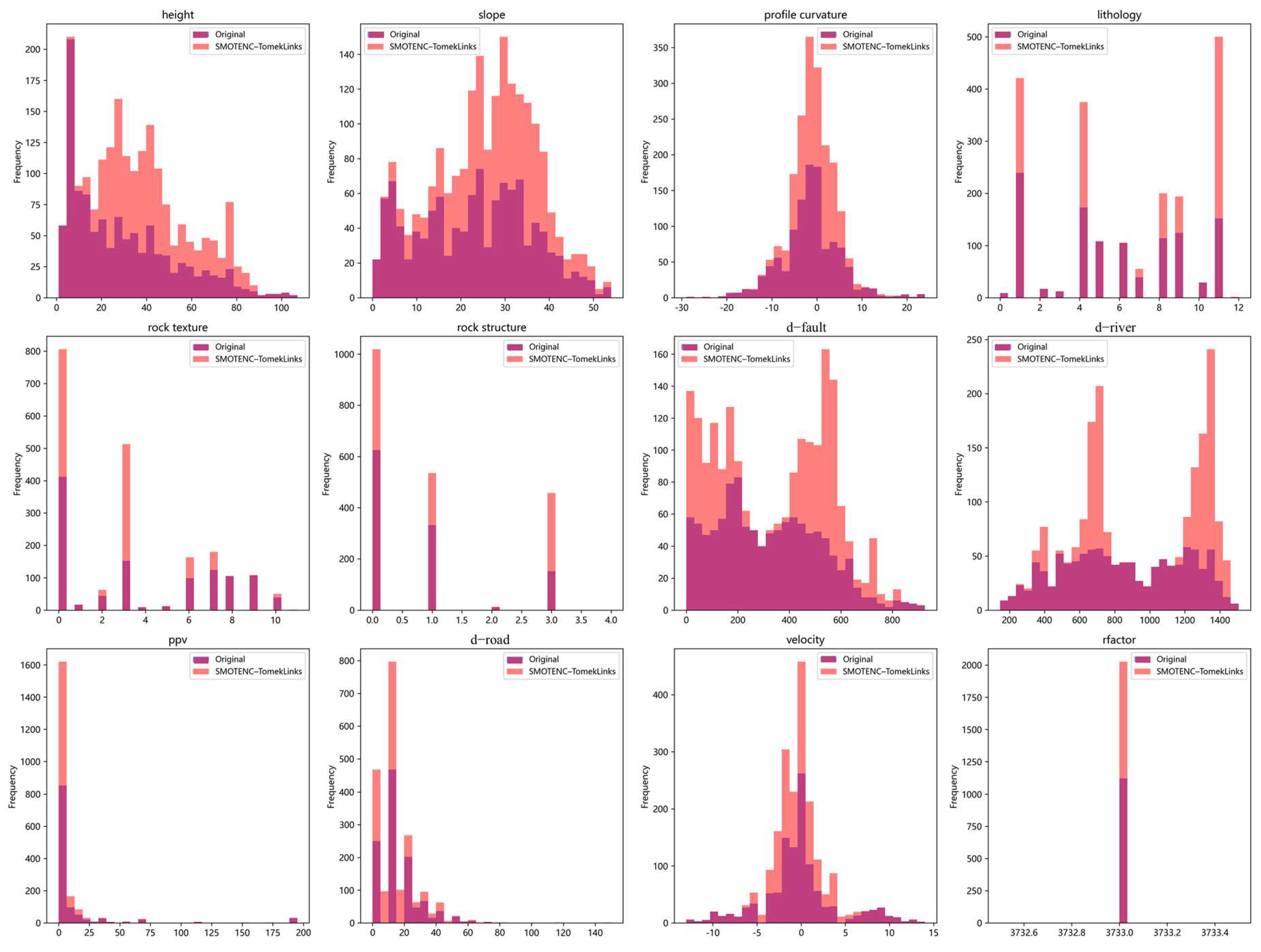
The SMOTENC–TomekLinks method is applied to resample the landslide samples. After resampling, the proportion of positive to negative instances approximates 1:1, as shown in the data distribution in
Figure 5.
3.4. Hyperparameter Optimization Model and Model Evaluation
In this study, we used a random search strategy for hyperparameter optimization within a predefined search space [
66]. This method randomly samples hyperparameters and combines them to train models, enabling efficient exploration of a broader configuration space within a fixed number of trials, thus mitigating the exponential increase in search time as the search space expands. The computational complexity is O(n), with n representing the maximum number of evaluations, which is set to 100 in this study.
The hyperparameter space included both discrete and continuous variables, such as learning rate, the number of estimators, minimum child weight, maximum depth, and sampling ratios, sampled from their respective distributions. The optimization process used the Hyperopt library and the TPE (Tree-structured Parzen Estimator) algorithm to identify the optimal hyperparameters that maximized model performance, evaluated using a composite loss function integrating the AUC, F1-score, and recall rate. This method enhances model generalization while maintaining efficiency by reducing unnecessary computations.
3.5. Model for Interpreting Landslide Susceptibility Mapping
SHAP is a game-theoretic method for explaining the output of machine learning models [
67]. It assigns an importance value to each feature, known as the SHAP value, which reflects the feature’s contribution to the model’s prediction for a given instance. The SHAP value is based on the Shapley value from cooperative game theory, which allocates the total outcome fairly among the players, in this context, the model’s features.
The SHAP value for a feature in a given prediction is calculated by evaluating all possible feature combinations and their contributions to the prediction. The process involves three steps:
Feature Subsets: For each feature, evaluate all possible subsets that can be combined with it.
Marginal Contribution: Compute the marginal contribution of the feature upon its inclusion in each subset.
Average Contributions: The SHAP value represents the average of these marginal contributions, weighted according to the number of subsets containing the feature.
Mathematically, the SHAP value
for feature
i in instance
x is given by Equation (2) [
28]:
where
N is the set of all features,
S is a subset of features that does not include
i,
f(
S) is the prediction using the feature subset
S, |
S| is the size of subset
S, and
n is the total number of features.
4. Results
4.1. Spatial Distribution Statistics of Slope Landslide Characteristic Data
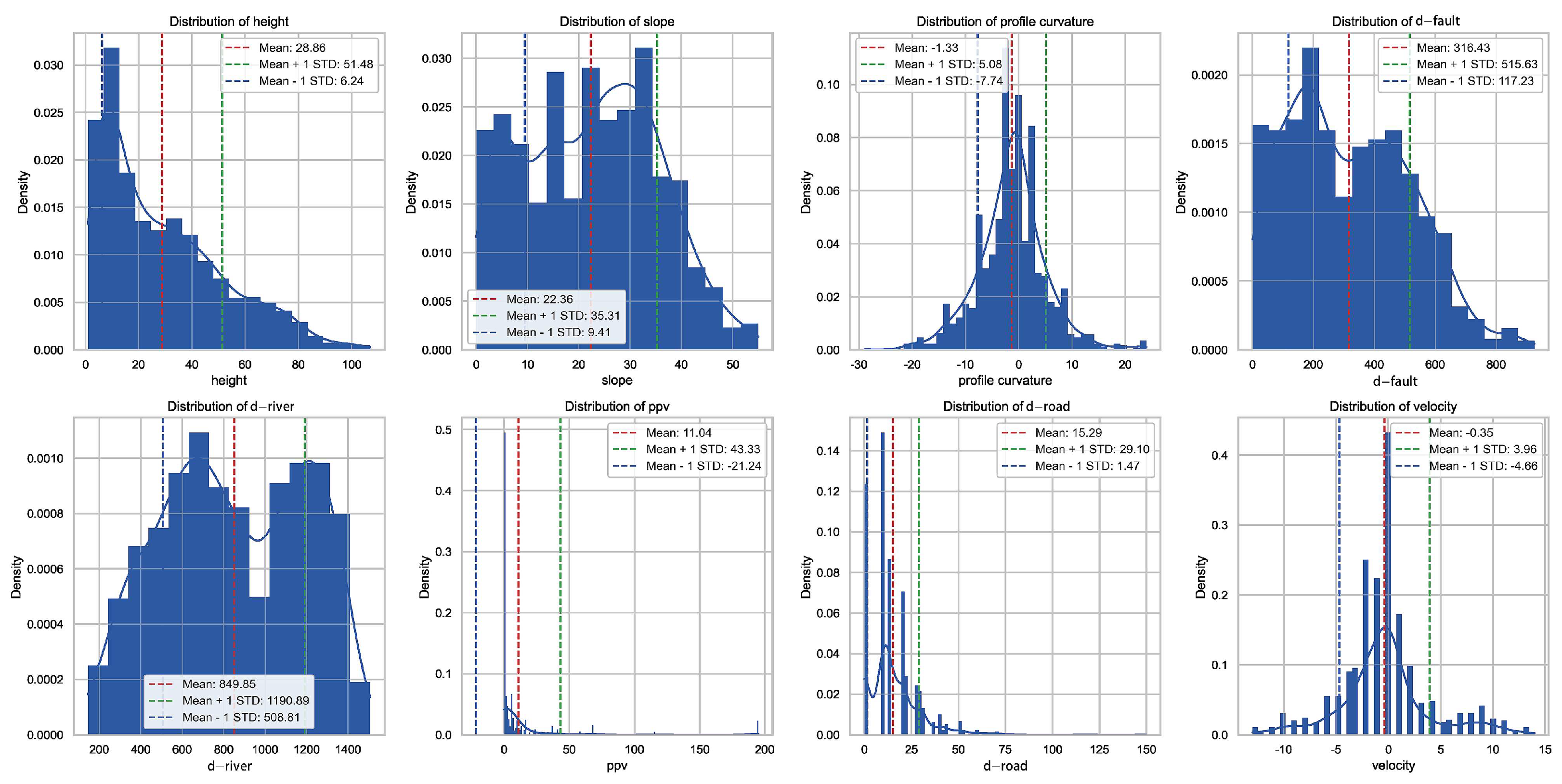
The distribution of numerical feature data is shown in
Figure 6. The maximum slope height is 107 m, with an average of 28.86 m, and most values are concentrated between 6.24 m and 51.48 m. The maximum slope is 55°, with an average of 22.36°, and most values are concentrated between 9.41° and 35.31°. The profile curvature ranges from a minimum of −29 to a maximum of 24, with an average of −1.33, mainly concentrated between −7.74 and 5.08. The maximum distance from the fault is 926 m, with an average of 316.43 m, and most values are concentrated between 117.23 m and 515.63 m. The minimum distance from the river is 146 m and the maximum value is 1507 m, with an average of 849.85 m, and most values are concentrated between 508.81 m and 1190.89 m. The peak particle vibration velocity is 195 m/s, with an average of 11.04 m/s. The maximum distance from the road is 150 m, with an average of 15.29 m, and most values are concentrated between 1.47 m and 29.10 m. The maximum subsidence rate is −13 mm/year, and the maximum uplift rate is 14 mm/year, with an average rate of −0.35 mm/year.
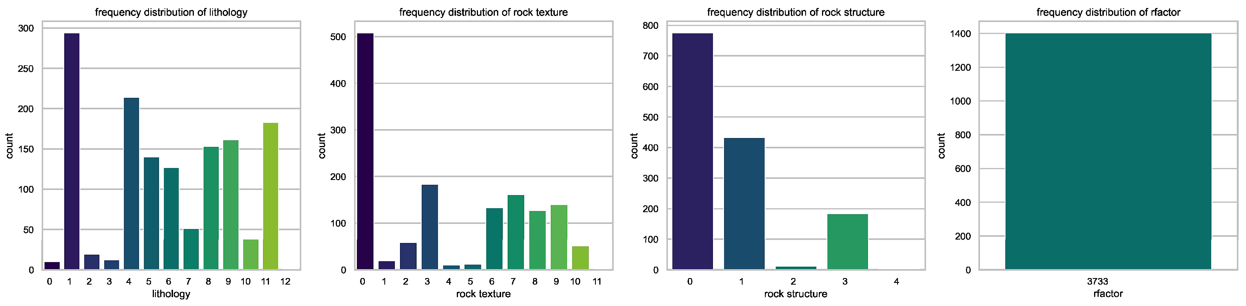
The distribution of categorical feature data is presented in
Figure 7. There are 12 types of lithology, with the top three being moderately black cloud granulite, strongly black cloud granulite, and the covered soil sand layer. There are 11 types of rock structures, with the top three being a medium-granular crystal texture, a single-grained texture, and a detrital texture. There are four types of rock structures, with the top three being blocky or weak igneous structure, massive structure, and fractured structure. Rainfall erosivity is a fixed value of 3733 MJ·mm·ha⁻
1·h⁻
1·a⁻
1, as rainfall intensity is consistent across the entire mining area.
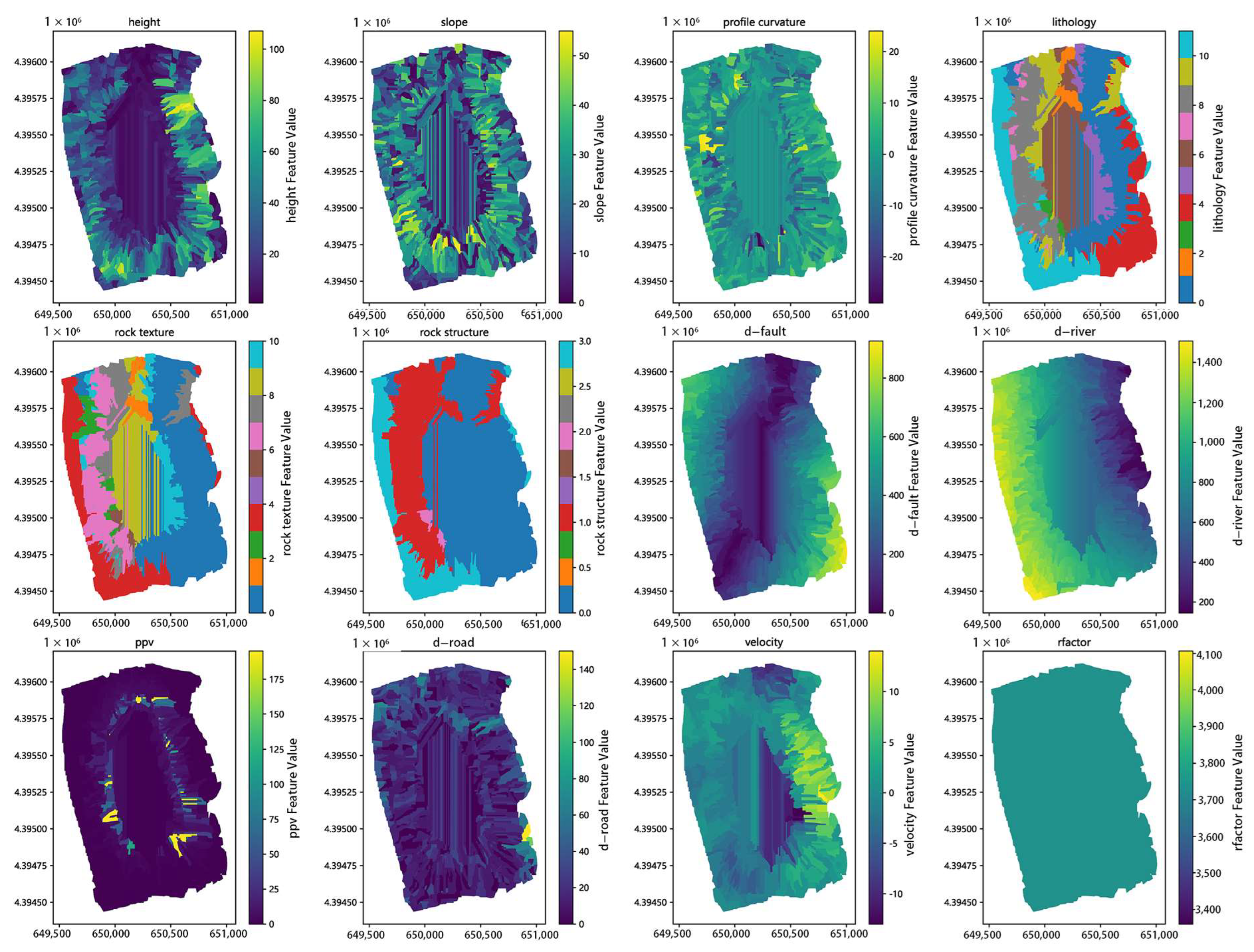
The spatial distribution of each feature datum is illustrated in
Figure 8.
4.2. Predisposing Factor Results
The 1403 slope units are split 8:2 between a training set and a test set. A label of 1 denotes a landslide, and a label of 0 denotes a non-landslide. The optimized LightGBM parameters and evaluation metrics are presented in
Table 2 and
Table 3.
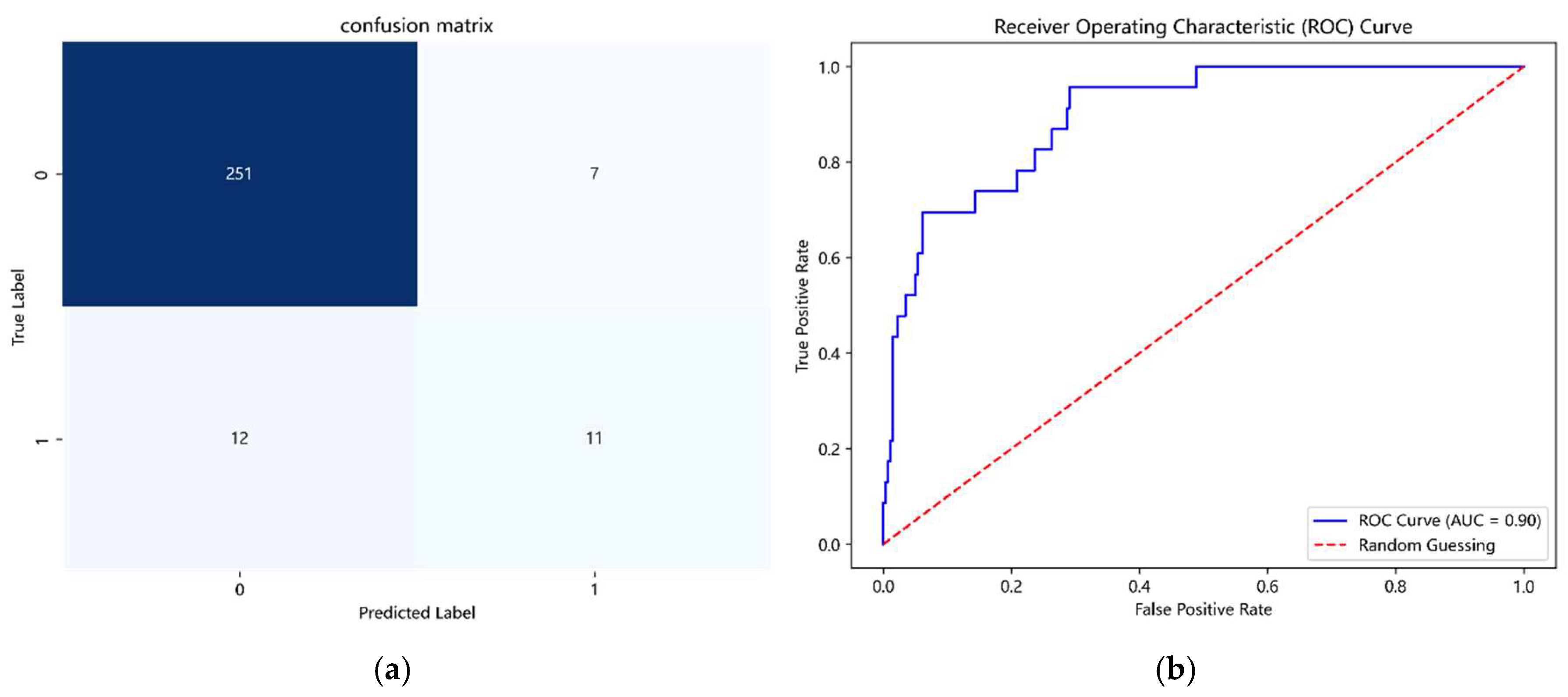
The confusion matrix and ROC curve are presented in
Figure 9.
The LightGBM parameters were optimized (
Table 2), and the model’s final performance on the test set is presented in
Table 3 and
Figure 9. The test set consists of 281 samples, including 23 actual landslide cases, of which 11 were correctly predicted. Among the 258 non-landslide cases, 251 were correctly predicted. The model achieved an F1-score of 93% and an AUC of 90%, demonstrating high predictive performance.
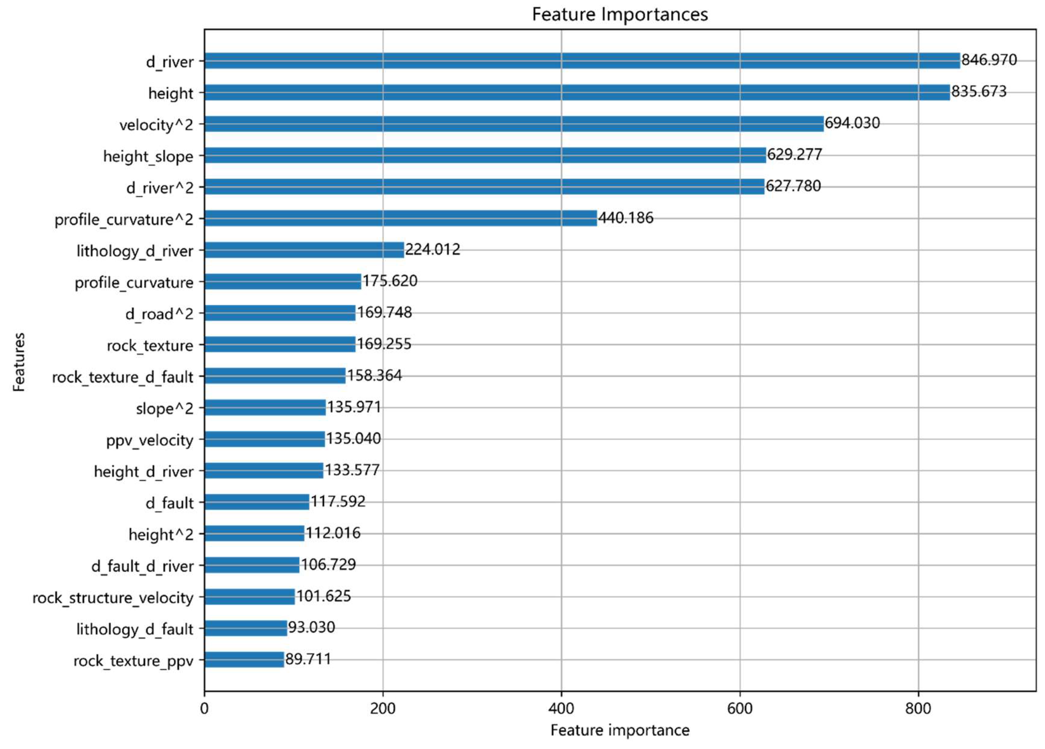
The LightGBM algorithm identifies the top 20 factors influencing landslide prediction, as shown in
Figure 10. The distance to the river exerts the most significant influence on landslide occurrence, with slope height being the second most influential factor. The quadratic of surface displacement change rate, the coupling factor of slope height and slope, the quadratic of distance from the river, and the quadratic of surface profile curvature also show high importance.
Among the 12 individual factors, the importance in influencing landslide occurrence is ranked as follows: distance from the river, slope height, profile curvature, rock texture, and distance from the fault.
In addition to the 12 individual factors, the top-ranking coupling factors (including self-coupling) are as follows: self-coupling of surface displacement change rate, slope height and slope, self-coupling of distance from river, self-coupling of profile curvature, lithology and distance from river, self-coupling of distance from road, rock texture and distance from fault, self-coupling of slope, maximum particle vibration velocity and surface displacement change rate, slope height and distance from river, self-coupling of slope height, distance from fault and distance from river, rock structure and surface displacement change rate, lithology and distance from fault, and rock texture and peak particle vibration velocity.
4.3. The Influence of Each Factor Value on the Output Results of the Model
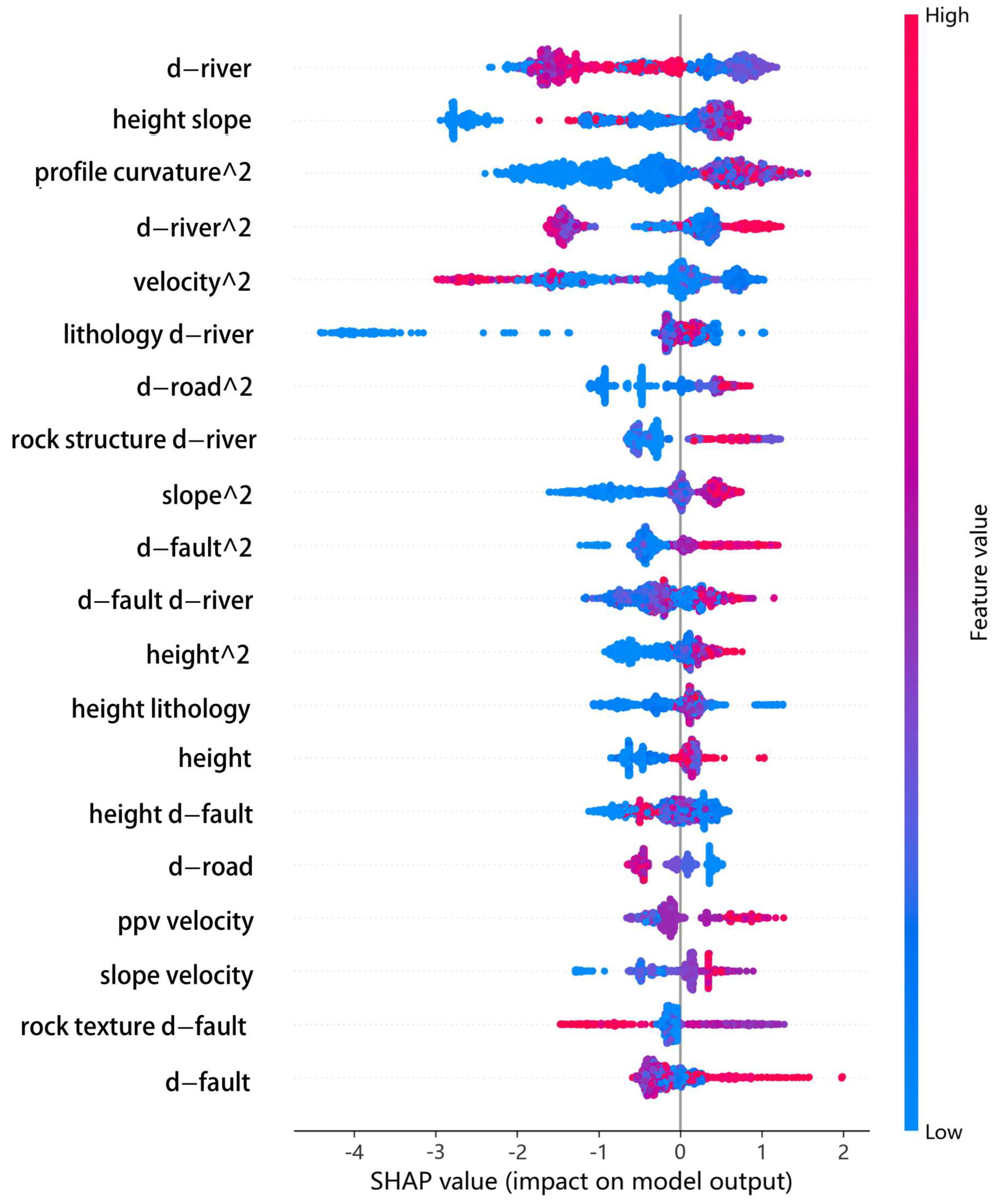
Figure 11 shows the top 20 factors identified by the SHAP algorithm, explaining the positive effect of slope characteristics on landslide prediction using LightGBM. In
Figure 11, color is used to represent the feature values, with red indicating high values and blue representing low values. A positive contribution to landslide prediction is shown by a SHAP value larger than 0; a negative contribution is indicated by a value less than 0. Each point corresponds to a slope sample. The figure shows that for the top three predisposing factors, a shorter distance to the river increases the likelihood of a landslide. A higher slope shape value, determined by slope height and slope angle, increases landslide susceptibility. A higher squared profile curvature value, indicating greater concavity and convexity of the slope profile, increases the likelihood of a landslide.
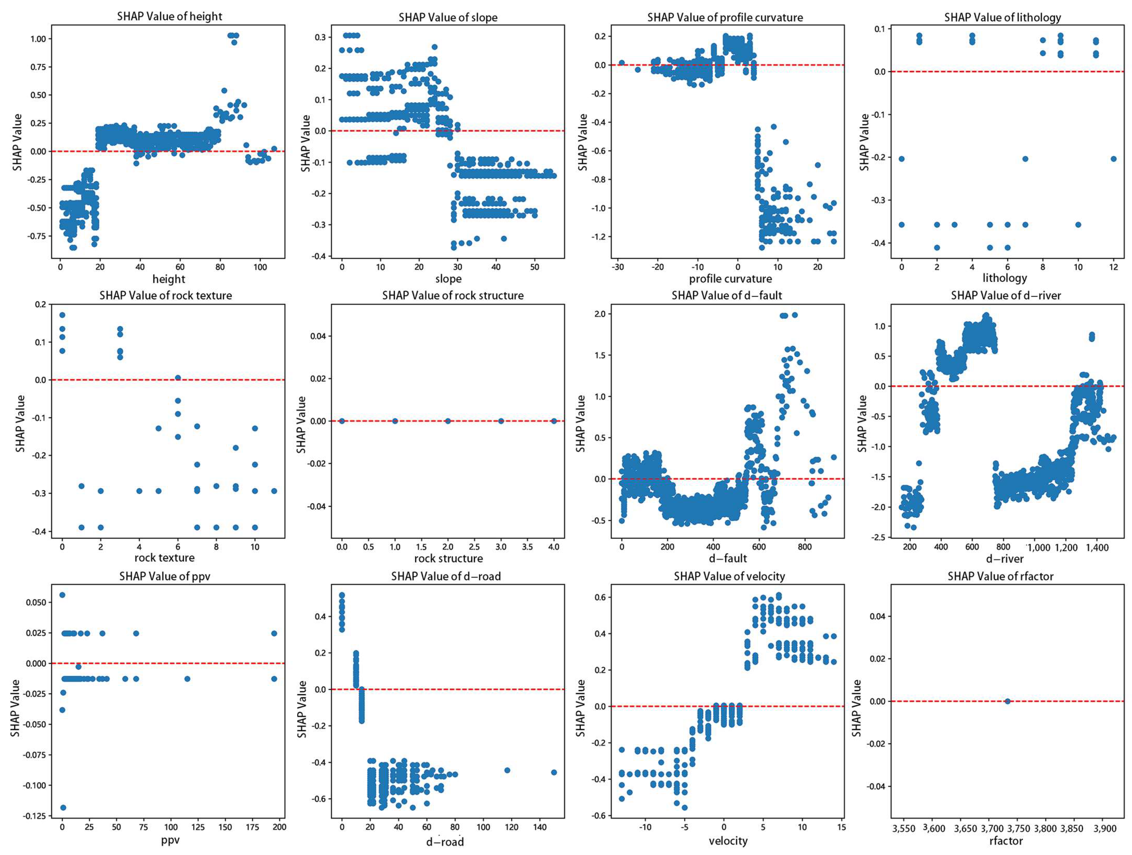
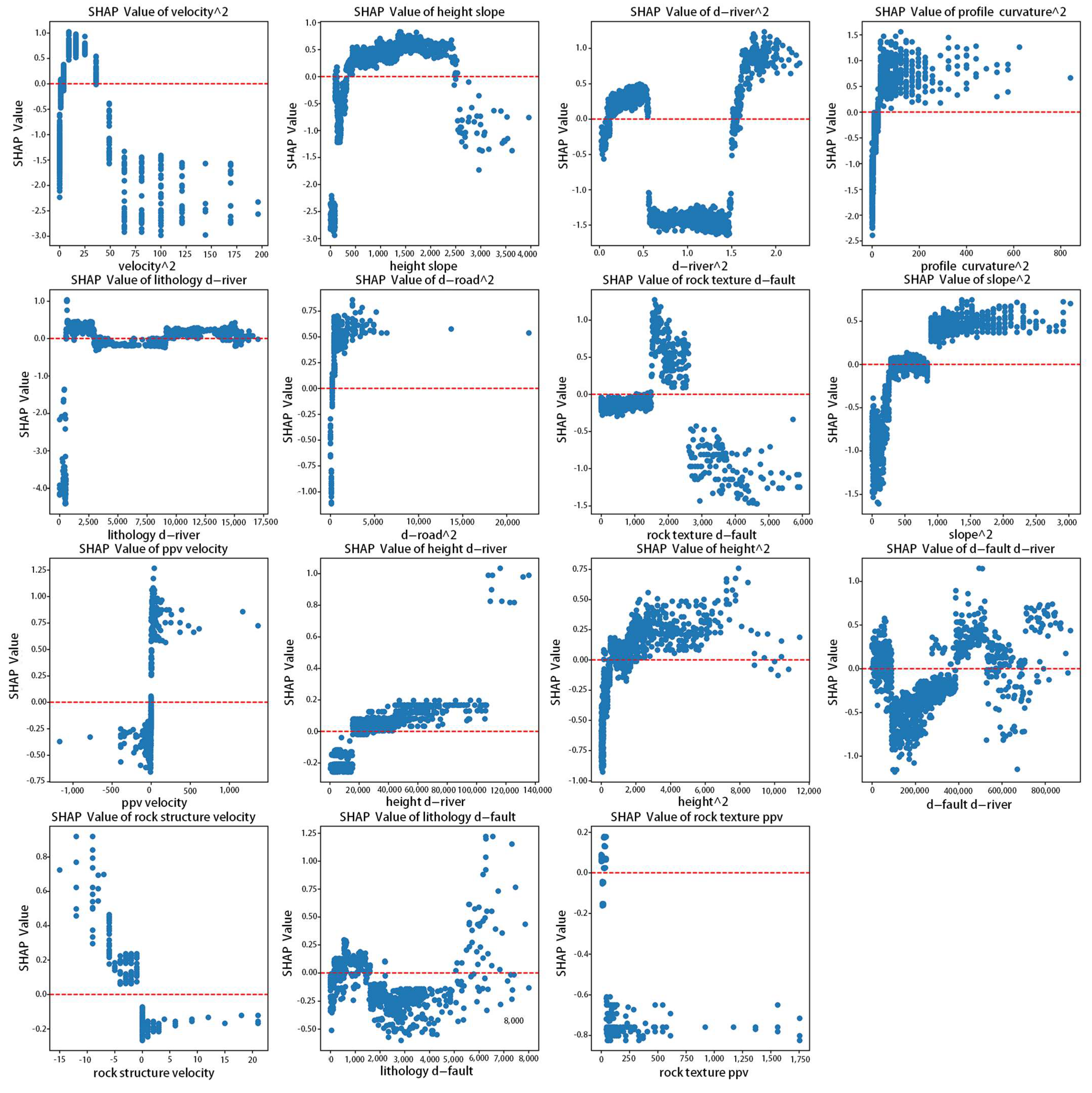
The positive and negative correlations between feature values and SHAP values help clarify the influence trend of each feature on slope stability. However, a more detailed analysis is needed to determine the specific range of each feature’s impact. The SHAP value distributions for single-factor features and for coupling and self-coupling factors are shown in
Figure 12 and
Figure 13, respectively.
From the single-factor characteristics in
Figure 12, it can be seen that slope stability is generally good when the slope height is below 20 m. Between 20 m and 80 m, the slope stability decreases, and between 80 m and 90 m, the risk of landslides increases sharply. A slope gradient of 28° serves as a threshold for slope stability in the Sijiaying mining area. For profile curvature, values between −5 and 5 are unfavorable to slope stability, while values greater than 5 are beneficial, and values below −5 indicate potential instability. In terms of lithology, moderately weathered black cloud granulite, strongly weathered black cloud granulite, dolomite, silicarenite, and covered soil sand layers are detrimental to slope stability. Among rock textures, the medium-granular crystal structure and single-grained structure are the primary instability factors. Rock structures show no significant effect on slope stability. When the distance from the fault is less than 180 m, it has little influence on slope stability, while distances between 180 m and 580 m have no discernible effect. Distances greater than 580 m are represented by sparse and non-representative sample points. Distances from the river between 400 m and 750 m negatively affect slope stability. The peak particle vibration velocity from blasting has no clear impact on slope stability. When the distance from the road is less than 10 m, it negatively affects slope stability. A surface displacement rate greater than 2.5 mm/year is unfavorable, with surface uplift being more likely to trigger landslides than surface subsidence in the Sijiaying mining area. The lack of spatial differentiation of rainfall erosivity in the mining area means that its influence on slope stability cannot be assessed.
The coupling characteristics shown in
Figure 13 reveal the following relationships: When the square of the surface displacement rate is between 10 and 40, slope stability is poor. A coupling value of slope height and slope between 500 and 2500 negatively impacts stability. The square of the distance from the river between 0.1 × 10
6 and 0.5 × 10
6 is also unfavorable to slope stability. When the square of the section curvature exceeds 50, slope stability is compromised. The coupling of lithology and distance from the river, in the range of 1000 to 2500, is detrimental to slope stability. A distance from the road squared less than 5000 indicates a risk of instability. The coupling of rock texture and distance from the fault is unfavorable when the value ranges from 1500 to 2500. A square of the slope greater than 900 also worsens slope stability. The coupling between the peak particle vibration velocity of blasting and the surface displacement rate tends to destabilize the slope when the slope is greater than 0. When the coupling of slope height and distance from the river exceeds 19,000, slope stability decreases. A square of slope height greater than 2000 is unfavorable for slope stability. When the coupling value of distance from the fault and distance from the river is less than 90,000, it negatively affects slope stability. Similarly, a coupling value of rock structure and surface displacement rate below 0 is detrimental to slope stability. The coupling of lithology and distance from the fault, within the range of 200 to 1500, also harms slope stability. Finally, the coupling of rock texture and the peak particle vibration velocity of blasting, when equal to 0, indicates that the medium-granular crystal structure is more prone to damage under blasting vibrations.
Comparing the relationship between landslide characteristic values and their corresponding SHAP values allows the identification of each feature’s impact on slope stability within defined numerical ranges. This approach helps establish the threshold intervals of characteristic values that negatively impact slope stability.
4.4. Global Diagnosis of Sliding Factors of Each Slope
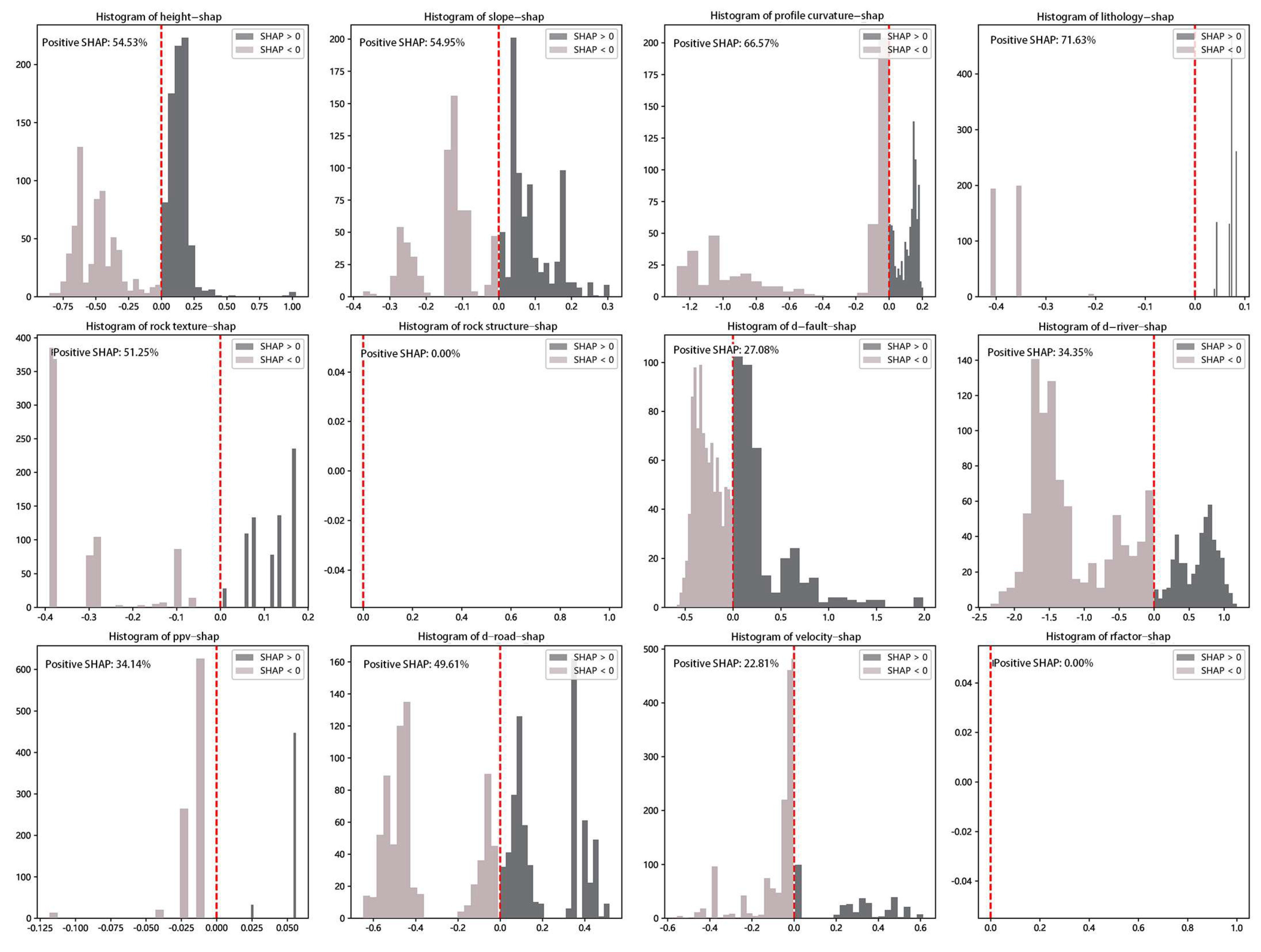
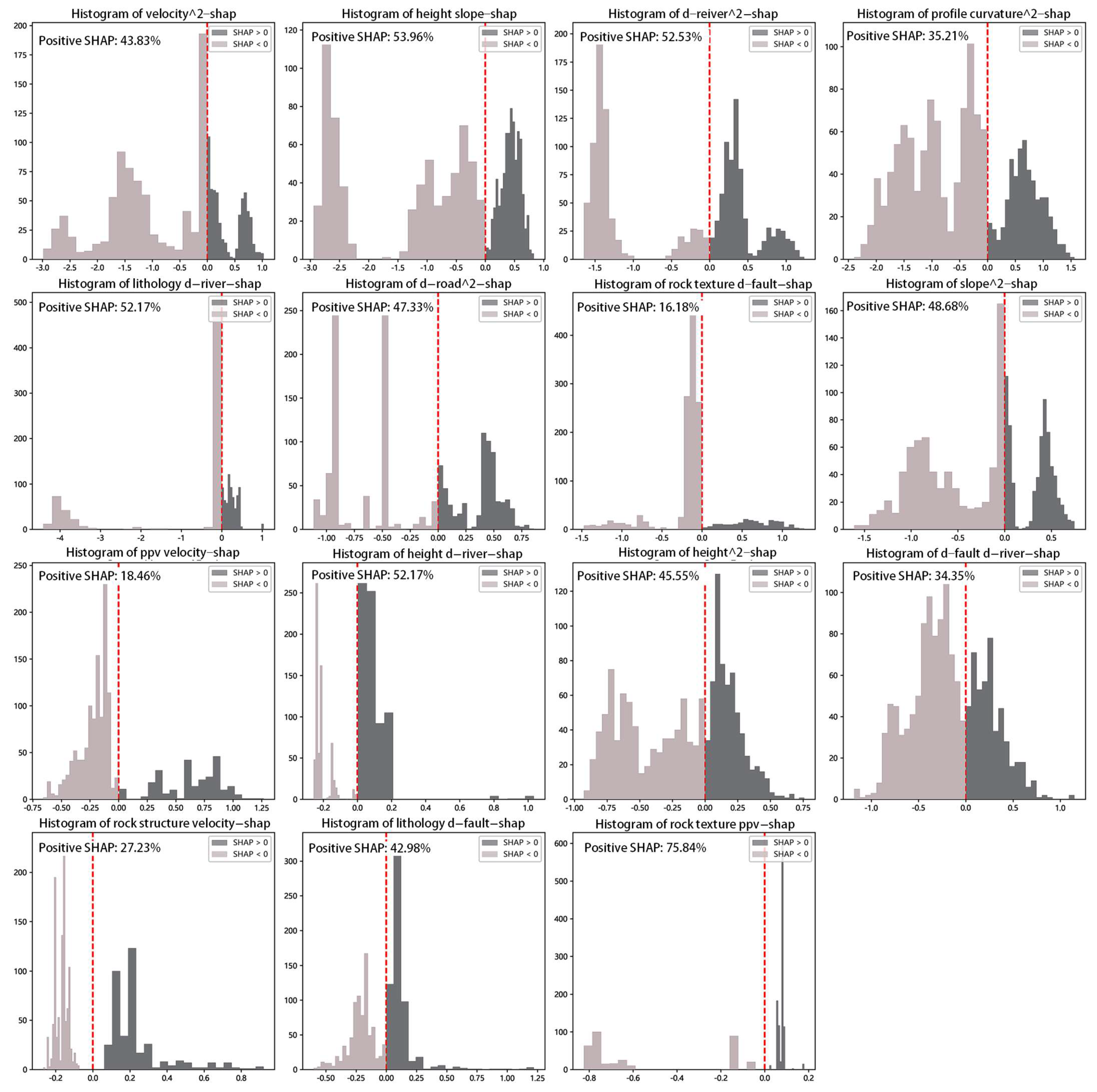
By analyzing the proportion of SHAP values greater than 0 across multiple samples, the overall impact of each feature on slope stability can be evaluated. A SHAP value greater than 0 signifies a positive effect of the feature on the likelihood of landslides in the predicted sample. The frequency distributions of SHAP values for single factors and coupling factors are presented in
Figure 14 and
Figure 15.
Figure 14 and
Figure 15 show that the single-factor characteristics with a SHAP value greater than 0 and a sample proportion greater than 50% include slope height, slope, profile curvature, lithology, and rock texture. The coupling factors include the interaction between slope height and slope, the self-coupling of distance from the river, the coupling of lithology and distance from the river, the coupling of slope height and distance from the river, and the interaction between rock texture and the peak particle vibration velocity of blasting.
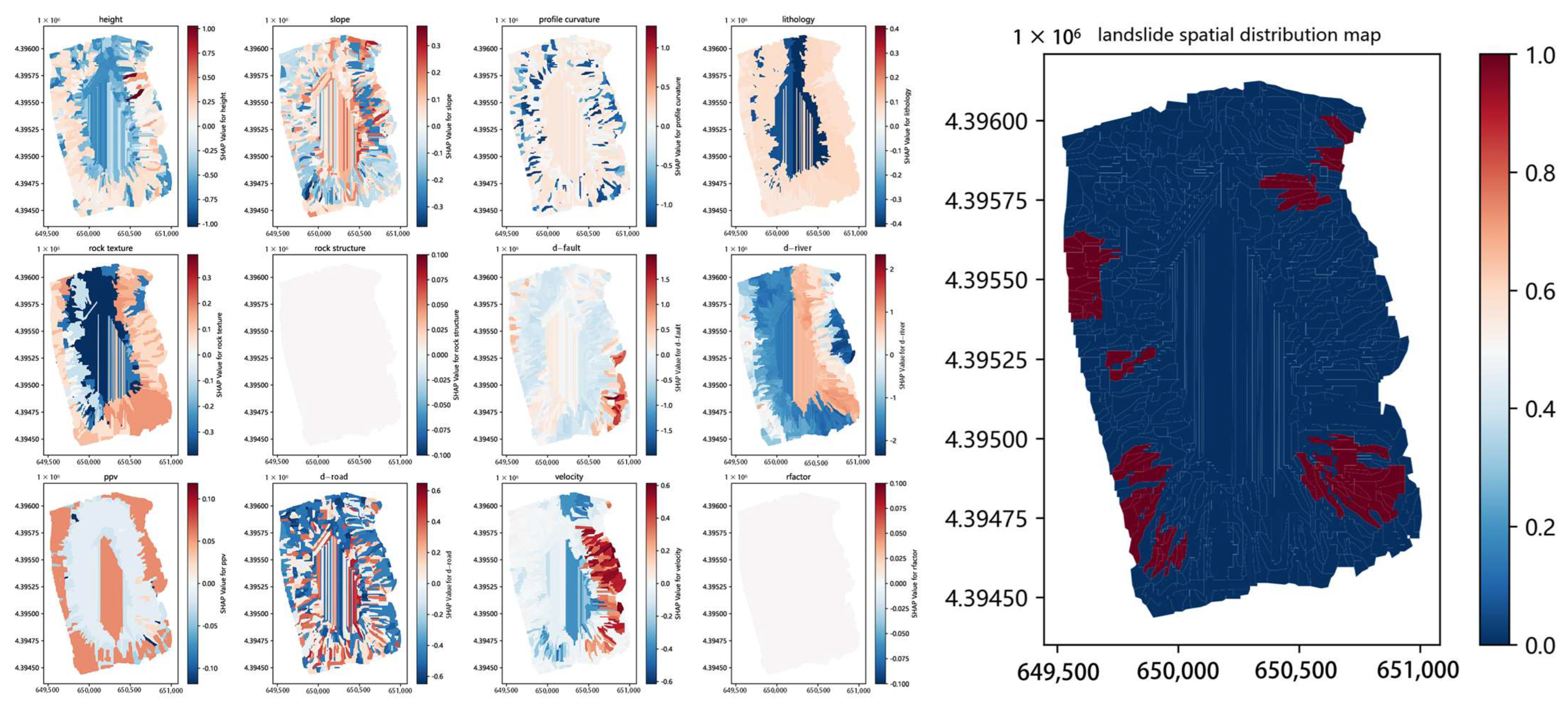
Figure 16 depicts the spatial distribution of SHAP values for each individual factor at the Sijiaying Iron Mine. This visualization allows for an intuitive understanding of how each single-factor characteristic influences the stability of the slope units, providing insights for targeted slope stability improvements.
As shown in the figure above, the red band represents characteristic values that negatively affect slope stability. The intensity of the red color corresponds to the magnitude of its influence on the likelihood of a slope landslide.
4.5. Determination of Key Sliding Factors of Single Slope
The generated landslide sensitivity map can be employed to assess the sliding characteristics of high-risk slopes in the Sijiaying mining area.
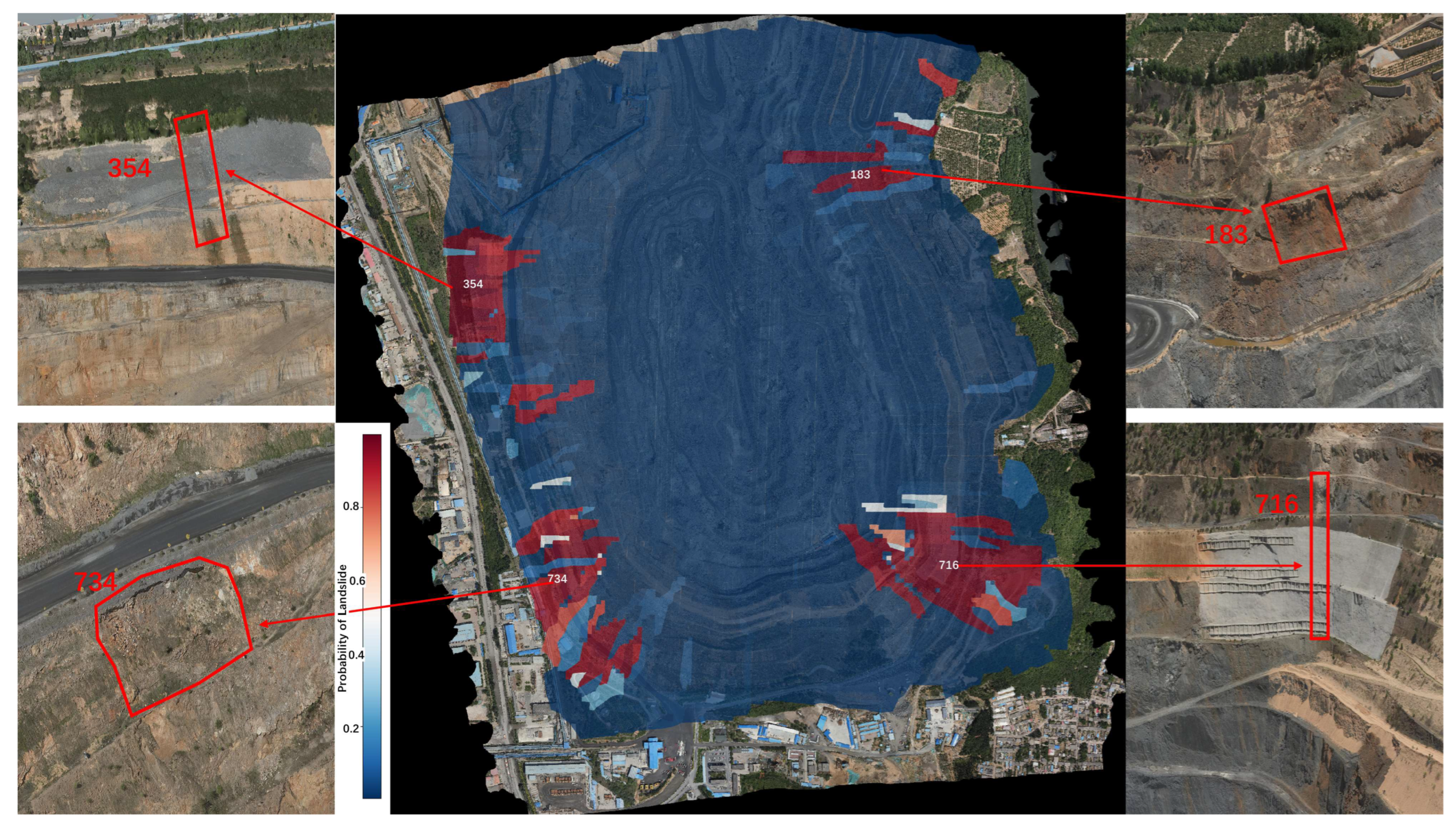
Figure 17 presents the landslide sensitivity map for the slopes in the Sijiaying mining area.
The red areas in the figure indicate landslide risk greater than 50%. The intensity of the red color corresponds to higher risk levels. The figure indicates that high-risk landslides are mainly concentrated in four regions, located at the four corners of the shallower sections of the mining area. These landslides are distributed approximately between exploration lines N8-N10 and N14-N16. Shallow overburden landslides are analyzed in conjunction with soil distribution in the shallow area (
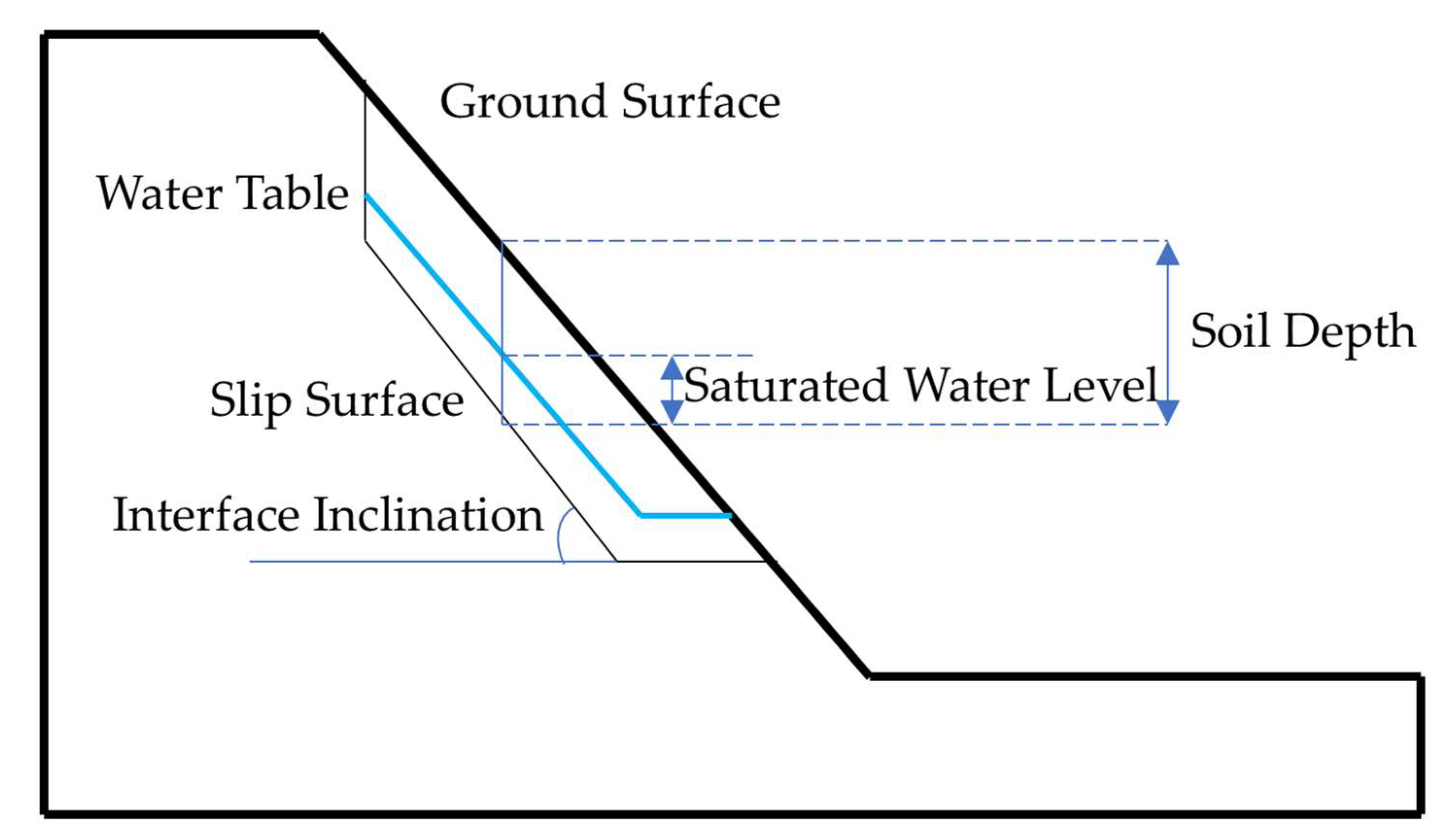
Figure 3) and the landslide mechanism (
Figure 18) [
68,
69]. Depending on soil type and the degree of saturation in soil or weathered soft rock, variations in rainfall intensity and duration alter the water level on the impermeable layer, increasing pore water pressure in the surface soil. Inadequate drainage and pressure relief increase the risk of landslides. Although the landslide-inducing factors selected in this study do not directly include these variables, they are indirectly related. Factors representing slope morphology (e.g., slope, profile curvature) influence rainfall infiltration. Comprehensive engineering geological factors (e.g., lithology, rock texture, rock structure, distance from faults, and distance from rivers) act as carriers of infiltrated rainwater and indirectly reflect soil water distribution under specific conditions. The surface displacement change rate is influenced by multiple factors. Based on the engineering context, it can be attributed to changes in groundwater levels.
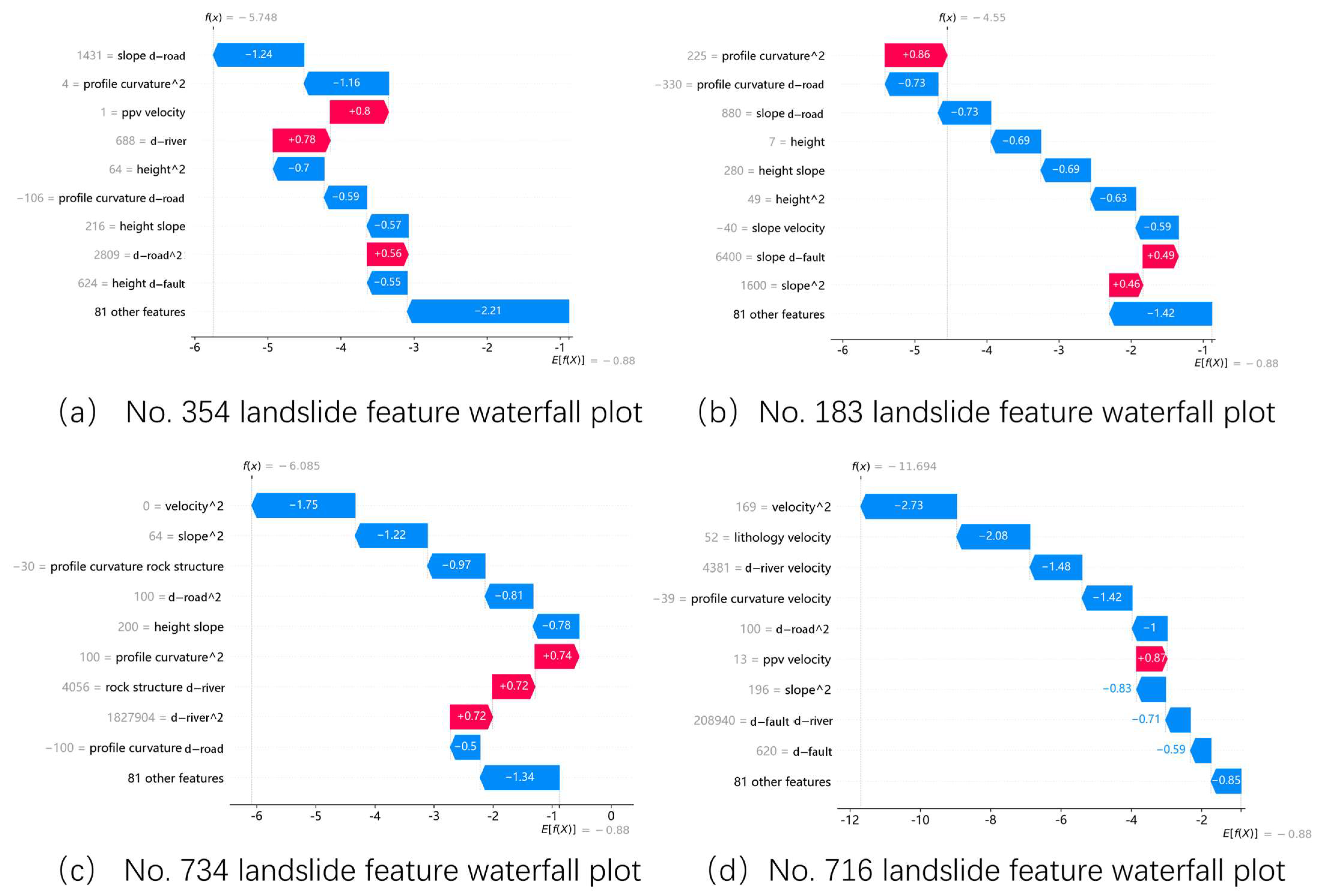
Slopes from these four regions were selected for individual slip factor analysis, and corresponding feature waterfall diagrams were created, as shown in
Figure 19.
The individual sample feature waterfall plot demonstrates the sequential accumulation of each feature’s SHAP value from the baseline value E[f(x)] to the final predicted value f(x).
Specifically, E[f(x)] denotes the average or expected value of the model’s output, serving as the baseline prediction. It represents the model’s average predicted value in the absence of specific input features and acts as the reference point for predictions, while f(x) is the actual predicted value for a specific input sample, calculated by the model after considering all input features. The SHAP value reveals whether each feature’s contribution increases or decreases from the baseline prediction E[f(x)] to the final prediction f(x). The red feature in the figure corresponds to the sliding characteristic of the slope sample, which is a critical factor for landslide prevention and mitigation.
As shown in
Figure 19a, the primary sliding characteristics of the No. 354 slope landslide on the northwest slope are the coupling between the maximum particle vibration velocity and the surface displacement change rate, as well as the distances from the river and the road. The peak particle vibration velocity and surface displacement change rate are both 1, indicating that the slope is highly sensitive to blasting vibrations and surface uplift. The distance from the river is 688 m, indicating that groundwater from the river significantly influences slope stability. The self-coupling value for the distance from the road is 2809, with a road distance of 53 m. Therefore, the influence of blasting vibrations must be controlled to prevent landslides. The slope in this area is situated between exploration lines N14 and N16. The thickness of the soil layer ranges from 53 m to 72 m. Based on the local soil classification (SW, ML, CL, GC), groundwater should be drained to reduce surface uplift. Additionally, roads on and below the slope should be protected.
As illustrated in
Figure 19b, the primary sliding characteristics of the No. 183 landslide on the northeast slope include self-coupling of profile curvature, coupling between slope and distance from the fault, and self-coupling of the slope. The self-coupling value of profile curvature is 1925 (with a profile curvature of −15), indicating a convex slope surface. The coupling value between the slope and the distance from the fault is 6400 (with a slope of 40° and a distance from the fault of 160 m), suggesting that the fault’s proximity to the slope negatively impacts its stability. To improve slope stability, flat slope treatment should be implemented. Additionally, based on the location of nearby faults, the slope angle should be adjusted to further enhance stability.
As shown in
Figure 19c, the primary sliding characteristics of the No. 734 slope landslide on the southwest slope include the self-coupling of profile curvature, rock structure, and the self-coupling of the distance from the river. The self-coupling value of profile curvature is 100, and the profile curvature is −10, suggesting a convex slope with a steep surface. The coupling value between rock structure and distance from the river is 4056. The rock structure is a 3 (fissure), and the distance from the river is 1352 m. This suggests that the fissure of the slope significantly affects its stability, particularly under the influence of river groundwater. The self-coupling value of the distance from the river is 1,827,904, with a distance of 1352 m, indicating that the slope is heavily influenced by proximity to the river. This suggests that controlling the slope landslide can be achieved by flattening the slope, reducing its curvature, and managing the development of slope cracks. Grouting treatment can be used to flatten the landslide surface and prevent rainfall from increasing groundwater pressure through crack infiltration. Additionally, the slope in this area is located between exploration lines N8 and N10. The thickness of the shallow soil layer ranges from 27 m to 58 m. Beneath the overburden layer lies a rock mass with well-developed fissures. When analyzing, attention should be given to the combined effect of rainfall on both the shallow soil and the fissured rock mass.
As shown in
Figure 19d, the primary sliding characteristics of the No. 716 slope landslide on the southeast slope include the coupling between the peak particle velocity and the rate of surface displacement change, which is 13. The peak particle velocity is 1 mm/s, and the surface displacement change rate is 13 mm/a uplift, indicating that the slope is sensitive to both blasting vibration and surface uplift. Thus, controlling blasting vibration is essential to prevent slope landslides, and groundwater drainage should be implemented to reduce surface uplift.
5. Discussion
The machine learning-based landslide sensitivity model predicts the likelihood of landslide occurrence in a specific area, while the interpretability method explores potential application scenarios for landslide sensitivity analysis. This approach offers a novel method for identifying both global and local key sliding factors in mine slopes. Technically, this method relies on machine learning and ‘black box’ explanation. First, machine learning is employed to assess the sensitivity of factors influencing landslides. These factors are primarily categorized into numerical and categorical types. Many algorithms face challenges when processing categorical data. Common methods for converting categorical data into numerical values include one-hot encoding and label encoding [
70]. While one-hot encoding resolves the order relationship between categories and is suitable for most machine learning algorithms, it can lead to the ‘curse of dimensionality’ with datasets containing many categories, increasing feature redundancy and making interpretation difficult [
71]. Label encoding uses integers to represent each category, which avoids increasing data dimensionality and saves storage space. However, label encoding introduces false ordinal relationships, causing machine learning algorithms to incorrectly assume that the distances between labels have practical significance, which can reduce model performance. Therefore, this study employs the tree-based LightGBM algorithm when using label encoding. The algorithm enhances support for categorical features, effectively mitigating issues caused by label encoding.
Secondly, mine slope landslides have limited sample sizes, and the imbalance between positive and negative samples in model training is a frequent problem. When the disparity between positive and negative samples is too large, the model may bias predictions toward non-landslide categories, neglecting the importance of landslide categories with fewer samples. This results in poor prediction performance for the underrepresented categories. Common evaluation metrics, such as accuracy, can be misleading since the model may predict the majority class for most instances, yielding a high accuracy despite poor performance on minority classes. Therefore, it is essential to use evaluation metrics better suited for imbalanced datasets, such as precision, recall, and F1-scores. Alternatively, the sample distribution can be adjusted through oversampling (increasing minority samples) or undersampling (reducing majority samples) to achieve a more balanced dataset. This study employs the SMOTENC–TomekLinks combined method to resample the landslide samples, achieving near balance and enhancing model performance and generalization.
Additionally, in selecting landslide influencing factors, this study comprehensively considers the four major categories: topography, engineering geology, ecological environment, and mining engineering. Among the geological factors, both macroscopic factors (faults) affecting rock mass stability and microscopic factors (rock texture and structure) are considered, with the latter introduced for the first time. Additionally, dynamic factors (surface displacement change rate), derived from long-term remote sensing data, are also incorporated. Since the influence of rainfall factors is largely uniform across all slopes within the mining area, it is treated as a constant in this study.
To maintain the integrity of the features during later model interpretation, this study does not account for data collinearity, provided that model accuracy remains sufficiently high. The final model can help researchers and decision-makers make informed decisions when analyzing the key landslide factors. However, it is crucial to emphasize that landslide analysis should not rely exclusively on the factors computed by the model; a comprehensive assessment, considering the actual on-site conditions, is required.
Open-pit mines cover a relatively small area in geospatial analysis, while landslide sensitivity analysis requires extensive geographic data. To address this issue, researchers have explored various approaches. Some researchers utilize data from multiple mines to train models, increasing the amount of training data and enhancing model generalization [
72]. Others enhance algorithms and integrate traditional slope safety factor evaluation metrics to improve slope stability assessment accuracy [
73]. Despite the widespread adoption of landslide sensitivity analysis methods [
74], data-driven susceptibility assessment approaches can only estimate the spatial likelihood of landslides but cannot predict their failure modes [
75]. Additionally, variations in data structures and algorithm models introduce significant uncertainty in prediction results [
76].
6. Conclusions
The objective of this study is to identify the critical factors affecting slope stability. The LightGBM algorithm is used to build the landslide sensitivity model, while the SHAP method is applied to evaluate each factor’s contribution to the predictions, offering both positive and negative impact values for further examination of the key sliding factors.
The outcomes indicate that the key factors influencing slope stability in the Sijiaying Iron Mine are distance from the river, slope height, profile curvature, rock texture, and distance from the fault. The key coupling factors include self-coupling of surface displacement change rate, slope height and slope, self-coupling of distance from the river, self-coupling of profile curvature, and lithology and distance from the river. The sliding and safety thresholds for the major elements affecting slope stability are determined by examining the link between each contributing factor and SHAP values. Slippage is more likely when the distance from the river is between 400 m and 750 m, while the slope remains stable when the height is below 20 m. The stability of section curvature is greater when the value exceeds 5. The medium-granular crystalline structure and single-grained texture of the rock are the primary factors contributing to slope instability. When the distance from the fault is between 180 m and 580 m, it has no significant impact on slope stability. At this stage, from a global perspective of the mine’s slopes, factors such as slope height, slope angle, profile curvature, lithology, and rock texture have already reached the threshold range unfavorable to slope stability. Road closeness, groundwater, and blasting vibration are the main reasons for sliding for the northwest slope, according to the analysis of individual slope landslides. The key sliding factors for the southwest slope are profile curvature, rock structure, and distance from the river. The northeast slope’s primary sliding factors are profile curvature, slope angle, and distance from the fault. The key sliding factors for the southeast slope are blasting vibration and groundwater.
In summary, the interpretability analysis based on the landslide sensitivity model effectively quantifies the key factors influencing slope failure in open-pit mines, offering a novel approach to stability analysis. Nevertheless, additional investigation is necessary to refine the method and enhance the model’s capacity for generalization, thereby augmenting its adaptability.
Author Contributions
Conceptualization, J.L. (Jiang Li) and Z.T.; methodology, J.L. (Jiang Li); software, J.L. (Jiang Li); validation, Z.T.; formal analysis, J.L. (Jiang Li); investigation, J.L. (Jiang Li), N.T., A.S. and J.L. (Jianshu Liu); resources, F.W. and W.L.; data curation, J.L. (Jiang Li); writing—original draft preparation, J.L. (Jiang Li); writing—review and editing, Z.T., N.T., A.S. and J.L. (Jianshu Liu); visualization, J.L. (Jiang Li); supervision, Z.T.; project administration, Z.T., F.W. and W.L. All authors have read and agreed to the published version of the manuscript.
Funding
This research received no external funding.
Data Availability Statement
The corresponding author can provide the necessary model upon request.
Acknowledgments
We would like to express our gratitude to the colleagues and students at the University of Science and Technology Beijing and Sijiaying Iron Mine for their invaluable support and insightful suggestions throughout the testing and writing phases of this manuscript.
Conflicts of Interest
Authors Fenglin Wang and Wantao Li are employed by the company Luanxian Sijiaying Iron Mine Co., Ltd. The remaining authors declare that the research was conducted in the absence of any commercial or financial relationships that could be construed as a potential conflict of interest.
References
- Deng, D.-P.; Li, L.; Wang, J.-F.; Zhao, L.-H. Limit Equilibrium Method for Rock Slope Stability Analysis by Using the Generalized Hoek–Brown Criterion. Int. J. Rock Mech. Min. Sci. 2016, 89, 176–184. [Google Scholar] [CrossRef]
- Faramarzi, L.; Zare, M.; Azhari, A.; Tabaei, M. Assessment of Rock Slope Stability at Cham-Shir Dam Power Plant Pit Using the Limit Equilibrium Method and Numerical Modeling. Bull. Eng. Geol. Environ. 2017, 76, 783–794. [Google Scholar] [CrossRef]
- Ishii, Y.; Ota, K.; Kuraoka, S.; Tsunaki, R. Evaluation of Slope Stability by Finite Element Method Using Observed Displacement of Landslide. Landslides 2012, 9, 335–348. [Google Scholar] [CrossRef]
- Liu, S.; Su, Z.; Li, M.; Shao, L. Slope Stability Analysis Using Elastic Finite Element Stress Fields. Eng. Geol. 2020, 273, 105673. [Google Scholar] [CrossRef]
- Dou, J.; Oguchi, T.; Hayakawa, Y.S.; Uchiyama, S.; Saito, H.; Paudel, U. GIS-Based Landslide Susceptibility Mapping Using a Certainty Factor Model and Its Validation in the Chuetsu Area, Central Japan. In Landslide Science for a Safer Geoenvironment; Sassa, K., Canuti, P., Yin, Y., Eds.; Springer International Publishing: Cham, Switzerland, 2014; pp. 419–424. ISBN 978-3-319-05049-2. [Google Scholar]
- Bui, D.T.; Lofman, O.; Revhaug, I.; Dick, O. Landslide Susceptibility Analysis in the Hoa Binh Province of Vietnam Using Statistical Index and Logistic Regression. Nat. Hazards 2011, 59, 1413–1444. [Google Scholar] [CrossRef]
- Lombardo, L.; Mai, P.M. Presenting Logistic Regression-Based Landslide Susceptibility Results. Eng. Geol. 2018, 244, 14–24. [Google Scholar] [CrossRef]
- Lee, S.; Hong, S.-M.; Jung, H.-S. A Support Vector Machine for Landslide Susceptibility Mapping in Gangwon Province, Korea. Sustainability 2017, 9, 48. [Google Scholar] [CrossRef]
- Yao, X.; Tham, L.G.; Dai, F.C. Landslide Susceptibility Mapping Based on Support Vector Machine: A Case Study on Natural Slopes of Hong Kong, China. Geomorphology 2008, 101, 572–582. [Google Scholar] [CrossRef]
- Fang, Z.; Wang, Y.; Peng, L.; Hong, H. Integration of Convolutional Neural Network and Conventional Machine Learning Classifiers for Landslide Susceptibility Mapping. Comput. Geosci. 2020, 139, 104470. [Google Scholar] [CrossRef]
- Wang, Y.; Fang, Z.; Hong, H. Comparison of Convolutional Neural Networks for Landslide Susceptibility Mapping in Yanshan County, China. Sci. Total Environ. 2019, 666, 975–993. [Google Scholar] [CrossRef]
- Ermini, L.; Catani, F.; Casagli, N. Artificial Neural Networks Applied to Landslide Susceptibility Assessment. Geomorphology 2005, 66, 327–343. [Google Scholar] [CrossRef]
- Gómez, H.; Kavzoglu, T. Assessment of Shallow Landslide Susceptibility Using Artificial Neural Networks in Jabonosa River Basin, Venezuela. Eng. Geol. 2005, 78, 11–27. [Google Scholar] [CrossRef]
- Pham, B.T.; Tien Bui, D.; Pourghasemi, H.R.; Indra, P.; Dholakia, M.B. Landslide Susceptibility Assesssment in the Uttarakhand Area (India) Using GIS: A Comparison Study of Prediction Capability of Naïve Bayes, Multilayer Perceptron Neural Networks, and Functional Trees Methods. Theor. Appl. Climatol. 2017, 128, 255–273. [Google Scholar] [CrossRef]
- Hong, H.; Liu, J.; Bui, D.T.; Pradhan, B.; Acharya, T.D.; Pham, B.T.; Zhu, A.-X.; Chen, W.; Ahmad, B.B. Landslide Susceptibility Mapping Using J48 Decision Tree with AdaBoost, Bagging and Rotation Forest Ensembles in the Guangchang Area (China). CATENA 2018, 163, 399–413. [Google Scholar] [CrossRef]
- Hong, H.; Liu, J.; Zhu, A.-X. Modeling Landslide Susceptibility Using LogitBoost Alternating Decision Trees and Forest by Penalizing Attributes with the Bagging Ensemble. Sci. Total Environ. 2020, 718, 137231. [Google Scholar] [CrossRef]
- Bien, T.X.; Iqbal, M.; Jamal, A.; Nguyen, D.D.; Van Phong, T.; Costache, R.; Ho, L.S.; Van Le, H.; Nguyen, H.B.T.; Prakash, I.; et al. Integration of Rotation Forest and Multiboost Ensemble Methods with Forest by Penalizing Attributes for Spatial Prediction of Landslide Susceptible Areas. Stoch. Environ. Res. Risk Assess. 2023, 37, 4641–4660. [Google Scholar] [CrossRef]
- Pham, B.T.; Jaafari, A.; Prakash, I.; Bui, D.T. A Novel Hybrid Intelligent Model of Support Vector Machines and the MultiBoost Ensemble for Landslide Susceptibility Modeling. Bull. Eng. Geol. Environ. 2019, 78, 2865–2886. [Google Scholar] [CrossRef]
- Wu, Y.; Ke, Y.; Chen, Z.; Liang, S.; Zhao, H.; Hong, H. Application of Alternating Decision Tree with AdaBoost and Bagging Ensembles for Landslide Susceptibility Mapping. CATENA 2020, 187, 104396. [Google Scholar] [CrossRef]
- Shao, X.; Ma, S.; Xu, C.; Zhou, Q. Effects of Sampling Intensity and Non-Slide/Slide Sample Ratio on the Occurrence Probability of Coseismic Landslides. Geomorphology 2020, 363, 107222. [Google Scholar] [CrossRef]
- Yang, C.; Liu, L.-L.; Huang, F.; Huang, L.; Wang, X.-M. Machine Learning-Based Landslide Susceptibility Assessment with Optimized Ratio of Landslide to Non-Landslide Samples. Gondwana Res. 2023, 123, 198–216. [Google Scholar] [CrossRef]
- Kavzoglu, T.; Kutlug Sahin, E.; Colkesen, I. Selecting Optimal Conditioning Factors in Shallow Translational Landslide Susceptibility Mapping Using Genetic Algorithm. Eng. Geol. 2015, 192, 101–112. [Google Scholar] [CrossRef]
- Liao, M.; Wen, H.; Yang, L. Identifying the Essential Conditioning Factors of Landslide Susceptibility Models under Different Grid Resolutions Using Hybrid Machine Learning: A Case of Wushan and Wuxi Counties, China. CATENA 2022, 217, 106428. [Google Scholar] [CrossRef]
- Galli, M.; Ardizzone, F.; Cardinali, M.; Guzzetti, F.; Reichenbach, P. Comparing Landslide Inventory Maps. Geomorphology 2008, 94, 268–289. [Google Scholar] [CrossRef]
- Corominas, J.; van Westen, C.; Frattini, P.; Cascini, L.; Malet, J.-P.; Fotopoulou, S.; Catani, F.; Van Den Eeckhaut, M.; Mavrouli, O.; Agliardi, F.; et al. Recommendations for the Quantitative Analysis of Landslide Risk. Bull. Eng. Geol. Environ. 2014, 73, 209–263. [Google Scholar] [CrossRef]
- Pradhan, B.; Dikshit, A.; Lee, S.; Kim, H. An Explainable AI (XAI) Model for Landslide Susceptibility Modeling. Appl. Soft Comput. 2023, 142, 110324. [Google Scholar] [CrossRef]
- Sun, D.; Chen, D.; Zhang, J.; Mi, C.; Gu, Q.; Wen, H. Landslide Susceptibility Mapping Based on Interpretable Machine Learning from the Perspective of Geomorphological Differentiation. Land 2023, 12, 1018. [Google Scholar] [CrossRef]
- Zhou, X.; Wen, H.; Li, Z.; Zhang, H.; Zhang, W. An Interpretable Model for the Susceptibility of Rainfall-Induced Shallow Landslides Based on SHAP and XGBoost. Geocarto Int. 2022, 37, 13419–13450. [Google Scholar] [CrossRef]
- Du, J.; Glade, T.; Woldai, T.; Chai, B.; Zeng, B. Landslide Susceptibility Assessment Based on an Incomplete Landslide Inventory in the Jilong Valley, Tibet, Chinese Himalayas. Eng. Geol. 2020, 270, 105572. [Google Scholar] [CrossRef]
- Maharaj, R.J. Landslide Processes and Landslide Susceptibility Analysis from an Upland Watershed: A Case Study from St. Andrew, Jamaica, West Indies. Eng. Geol. 1993, 34, 53–79. [Google Scholar] [CrossRef]
- Vakhshoori, V.; Pourghasemi, H.R.; Zare, M.; Blaschke, T. Landslide Susceptibility Mapping Using GIS-Based Data Mining Algorithms. Water 2019, 11, 2292. [Google Scholar] [CrossRef]
- Saito, H.; Nakayama, D.; Matsuyama, H. Comparison of Landslide Susceptibility Based on a Decision-Tree Model and Actual Landslide Occurrence: The Akaishi Mountains, Japan. Geomorphology 2009, 109, 108–121. [Google Scholar] [CrossRef]
- Samia, J.; Temme, A.; Bregt, A.; Wallinga, J.; Guzzetti, F.; Ardizzone, F.; Rossi, M. Characterization and Quantification of Path Dependency in Landslide Susceptibility. Geomorphology 2017, 292, 16–24. [Google Scholar] [CrossRef]
- Segoni, S.; Pappafico, G.; Luti, T.; Catani, F. Landslide Susceptibility Assessment in Complex Geological Settings: Sensitivity to Geological Information and Insights on Its Parameterization. Landslides 2020, 17, 2443–2453. [Google Scholar] [CrossRef]
- Nsengiyumva, J.B.; Luo, G.; Amanambu, A.C.; Mind’je, R.; Habiyaremye, G.; Karamage, F.; Ochege, F.U.; Mupenzi, C. Comparing Probabilistic and Statistical Methods in Landslide Susceptibility Modeling in Rwanda/Centre-Eastern Africa. Sci. Total Environ. 2019, 659, 1457–1472. [Google Scholar] [CrossRef] [PubMed]
- Yu, X.; Zhang, K.; Song, Y.; Jiang, W.; Zhou, J. Study on Landslide Susceptibility Mapping Based on Rock–Soil Characteristic Factors. Sci. Rep. 2021, 11, 15476. [Google Scholar] [CrossRef]
- Borrelli, L.; Ciurleo, M.; Gullà, G. Shallow Landslide Susceptibility Assessment in Granitic Rocks Using GIS-Based Statistical Methods: The Contribution of the Weathering Grade Map. Landslides 2018, 15, 1127–1142. [Google Scholar] [CrossRef]
- He, Y.; Zhao, Z.; Zhu, Q.; Liu, T.; Zhang, Q.; Yang, W.; Zhang, L.; Wang, Q. An Integrated Neural Network Method for Landslide Susceptibility Assessment Based on Time-Series InSAR Deformation Dynamic Features. Int. J. Digit. Earth 2024, 17, 2295408. [Google Scholar] [CrossRef]
- Mead, S.; Magill, C.; Hilton, J. Rain-Triggered Lahar Susceptibility Using a Shallow Landslide and Surface Erosion Model. Geomorphology 2016, 273, 168–177. [Google Scholar] [CrossRef]
- Kritikos, T.; Davies, T. Assessment of Rainfall-Generated Shallow Landslide/Debris-Flow Susceptibility and Runout Using a GIS-Based Approach: Application to Western Southern Alps of New Zealand. Landslides 2015, 12, 1051–1075. [Google Scholar] [CrossRef]
- Liu, F.; Chen, W.; Yang, Z.; Deng, W.; Li, H.; Yang, T. Landslide Characteristics and Stability Control of Bedding Rock Slope: A Case Study in the Sijiaying Open-Pit Mine. Min. Metall. Explor. 2024, 41, 3007–3022. [Google Scholar] [CrossRef]
- Devkota, K.C.; Regmi, A.D.; Pourghasemi, H.R.; Yoshida, K.; Pradhan, B.; Ryu, I.C.; Dhital, M.R.; Althuwaynee, O.F. Landslide Susceptibility Mapping Using Certainty Factor, Index of Entropy and Logistic Regression Models in GIS and Their Comparison at Mugling–Narayanghat Road Section in Nepal Himalaya. Nat. Hazards 2013, 65, 135–165. [Google Scholar] [CrossRef]
- Yue, T.; Yin, S.; Xie, Y.; Yu, B.; Liu, B. Rainfall Erosivity Mapping over Mainland China Based on High-Density Hourly Rainfall Records. Earth Syst. Sci. Data 2022, 14, 665–682. [Google Scholar] [CrossRef]
- Ma, S.; Shao, X.; Xu, C. Landslide Susceptibility Mapping in Terms of the Slope-Unit or Raster-Unit, Which Is Better? J. Earth Sci. 2023, 34, 386–397. [Google Scholar] [CrossRef]
- Wang, F.; Xu, P.; Wang, C.; Wang, N.; Jiang, N. Application of a GIS-Based Slope Unit Method for Landslide Susceptibility Mapping along the Longzi River, Southeastern Tibetan Plateau, China. Int. J. Geo-Inf. 2017, 6, 172. [Google Scholar] [CrossRef]
- Gorsevski, P.V.; Gessler, P.E.; Foltz, R.B.; Elliot, W.J. Spatial Prediction of Landslide Hazard Using Logistic Regression and ROC Analysis. Trans. GIS 2006, 10, 395–415. [Google Scholar] [CrossRef]
- Bradley, A.P. The Use of the Area under the ROC Curve in the Evaluation of Machine Learning Algorithms. Pattern Recognit. 1997, 30, 1145–1159. [Google Scholar] [CrossRef]
- Jiménez-Valverde, A. Insights into the Area under the Receiver Operating Characteristic Curve (AUC) as a Discrimination Measure in Species Distribution Modelling. Glob. Ecol. Biogeogr. 2012, 21, 498–507. [Google Scholar] [CrossRef]
- Wang, H.; Zhang, L.; Yin, K.; Luo, H.; Li, J. Landslide Identification Using Machine Learning. Geosci. Front. 2021, 12, 351–364. [Google Scholar] [CrossRef]
- Xu, S.; Song, Y.; Hao, X. A Comparative Study of Shallow Machine Learning Models and Deep Learning Models for Landslide Susceptibility Assessment Based on Imbalanced Data. Forests 2022, 13, 1908. [Google Scholar] [CrossRef]
- Li, L.; Lan, H.; Guo, C.; Zhang, Y.; Li, Q.; Wu, Y. A Modified Frequency Ratio Method for Landslide Susceptibility Assessment. Landslides 2017, 14, 727–741. [Google Scholar] [CrossRef]
- Klüver, J. A Mathematical Theory of Communication: Meaning, Information, and Topology. Complexity 2011, 16, 10–26. [Google Scholar] [CrossRef]
- Sun, D.; Wu, X.; Wen, H.; Gu, Q. A LightGBM-Based Landslide Susceptibility Model Considering the Uncertainty of Non-Landslide Samples. Geomat. Nat. Hazards Risk 2023, 14, 2213807. [Google Scholar] [CrossRef]
- Goetz, J.N.; Brenning, A.; Petschko, H.; Leopold, P. Evaluating Machine Learning and Statistical Prediction Techniques for Landslide Susceptibility Modeling. Comput. Geosci. 2015, 81, 1–11. [Google Scholar] [CrossRef]
- Friedman, J.H. Greedy Function Approximation: A Gradient Boosting Machine. Ann. Stat. 2001, 29, 1189–1232. [Google Scholar] [CrossRef]
- Sahin, E.K. Comparative Analysis of Gradient Boosting Algorithms for Landslide Susceptibility Mapping. Geocarto Int. 2022, 37, 2441–2465. [Google Scholar] [CrossRef]
- Sun, D.; Wu, X.; Wen, H.; Shi, S.; Gu, Q. Improving Generalization Performance of Landslide Susceptibility Model Considering Spatial Heterogeneity by Using the Geomorphic Label-Based LightGBM. Bull. Eng. Geol. Environ. 2024, 83, 361. [Google Scholar] [CrossRef]
- Saber, M.; Boulmaiz, T.; Guermoui, M.; Abdrabo, K.I.; Kantoush, S.A.; Sumi, T.; Boutaghane, H.; Nohara, D.; Mabrouk, E. Examining LightGBM and CatBoost Models for Wadi Flash Flood Susceptibility Prediction. Geocarto Int. 2022, 37, 7462–7487. [Google Scholar] [CrossRef]
- Youssef, K.; Shao, K.; Moon, S.; Bouchard, L.-S. Landslide Susceptibility Modeling by Interpretable Neural Network. Commun. Earth Environ. 2023, 4, 162. [Google Scholar] [CrossRef]
- Bao, F.; Deng, Y.; Kong, Y.; Ren, Z.; Suo, J.; Dai, Q. Learning Deep Landmarks for Imbalanced Classification. IEEE Trans. Neural Netw. Learn. Syst. 2020, 31, 2691–2704. [Google Scholar] [CrossRef]
- Bugnon, L.A.; Yones, C.; Milone, D.H.; Stegmayer, G. Deep Neural Architectures for Highly Imbalanced Data in Bioinformatics. IEEE Trans. Neural Netw. Learn. Syst. 2020, 31, 2857–2867. [Google Scholar] [CrossRef]
- Dablain, D.; Krawczyk, B.; Chawla, N.V. DeepSMOTE: Fusing Deep Learning and SMOTE for Imbalanced Data. IEEE Trans. Neural Netw. Learn. Syst. 2023, 34, 6390–6404. [Google Scholar] [CrossRef]
- Batista, G.E.A.P.A.; Prati, R.C.; Monard, M.C. A Study of the Behavior of Several Methods for Balancing Machine Learning Training Data. SIGKDD Explor. Newsl. 2004, 6, 20–29. [Google Scholar] [CrossRef]
- Pereira, R.M.; Costa, Y.M.G.; Silla, J.C.N. MLTL: A multi-label approach for the Tomek Link undersampling algorithm; MLTL: Tomek Link undersampling algorithm. Neurocomputing 2020, 383, 95–105. [Google Scholar] [CrossRef]
- Lee, Y.W.; Choi, J.W.; Shin, E.-H. Machine Learning Model for Diagnostic Method Prediction in Parasitic Disease Using Clinical Information. Expert Syst. Appl. 2021, 185, 115658. [Google Scholar] [CrossRef]
- Yang, L.; Shami, A. On Hyperparameter Optimization of Machine Learning Algorithms: Theory and Practice. Neurocomputing 2020, 415, 295–316. [Google Scholar] [CrossRef]
- Lundberg, S. A Unified Approach to Interpreting Model Predictions. arXiv 2017, arXiv:1705.07874. [Google Scholar]
- Di, B.; Stamatopoulos, C.A.; Stamatopoulos, A.C.; Liu, E.; Balla, L. Proposal, Application and Partial Validation of a Simplified Expression Evaluating the Stability of Sandy Slopes under Rainfall Conditions. Geomorphology 2021, 395, 107966. [Google Scholar] [CrossRef]
- Take, W.A.; Bolton, M.D.; Wong, P.C.P.; Yeung, F.J. Evaluation of Landslide Triggering Mechanisms in Model Fill Slopes. Landslides 2004, 1, 173–184. [Google Scholar] [CrossRef]
- Xiong, Y.; Zhou, Y.; Wang, F.; Wang, S.; Wang, Z.; Ji, J.; Wang, J.; Zou, W.; You, D.; Qin, G. A Novel Intelligent Method Based on the Gaussian Heatmap Sampling Technique and Convolutional Neural Network for Landslide Susceptibility Mapping. Remote Sens. 2022, 14, 2866. [Google Scholar] [CrossRef]
- Cerda, P.; Varoquaux, G. Encoding High-Cardinality String Categorical Variables. IEEE Trans. Knowl. Data Eng. 2022, 34, 1164–1176. [Google Scholar] [CrossRef]
- Wang, H.; Yang, T.; Wang, Y.; Zhao, Y.; Niu, P.; Zhang, P. Landslide Susceptibility Mapping and Similar Case Matching Based on Case Library: A Case Study of Xinjing Landslide, China. Geomat. Nat. Hazards Risk 2024, 15, 2413697. [Google Scholar] [CrossRef]
- Jiang, S.; Li, J.; Zhang, S.; Gu, Q.; Lu, C.; Liu, H. Landslide Risk Prediction by Using GBRT Algorithm: Application of Artificial Intelligence in Disaster Prevention of Energy Mining. Process Saf. Environ. Prot. 2022, 166, 384–392. [Google Scholar] [CrossRef]
- Lima, P.; Steger, S.; Glade, T.; Murillo-García, F.G. Literature Review and Bibliometric Analysis on Data-Driven Assessment of Landslide Susceptibility. J. Mt. Sci. 2022, 19, 1670–1698. [Google Scholar] [CrossRef]
- Lima, P.; Steger, S.; Glade, T.; Mergili, M. Conventional Data-Driven Landslide Susceptibility Models May Only Tell Us Half of the Story: Potential Underestimation of Landslide Impact Areas Depending on the Modeling Design. Geomorphology 2023, 430, 108638. [Google Scholar] [CrossRef]
- Xing, Y.; Chen, Y.; Huang, S.; Xie, W.; Wang, P.; Xiang, Y. Research on the Uncertainty of Landslide Susceptibility Prediction Using Various Data-Driven Models and Attribute Interval Division. Remote Sens. 2023, 15, 2149. [Google Scholar] [CrossRef]
Figure 1.
The geographical location of the study area.
Figure 1.
The geographical location of the study area.
Figure 2.
Landslide inventory maps for the study area.
Figure 2.
Landslide inventory maps for the study area.
Figure 3.
Distribution of soil sand layer.
Figure 3.
Distribution of soil sand layer.
Figure 4.
Technical flowchart of this study.
Figure 4.
Technical flowchart of this study.
Figure 5.
The data distribution before and after resampling.
Figure 5.
The data distribution before and after resampling.
Figure 6.
The specific distribution of numerical feature data.
Figure 6.
The specific distribution of numerical feature data.
Figure 7.
The distribution of categorical feature data. Lithology: 0—medium–coarse gravel quartz sandstone; 1—moderately weathered black cloud granulite; 2—metamorphic gabbro; 3—basal conglomerate; 4—strongly weathered black cloud granulite; 5—micro-weathered black cloud granulite; 6—mixed black cloud granulite; 7—flint dolomite; 8—dolomite; 9—silicarenite; 10—silicarenite and dolomite interbedded; 11—covered soil sand layer. Rock texture: 0—medium-granular crystal structure; 1—medium- to coarse-grained structure; 2—metasomatic recrystallized microcrystalline structure; 3—single-grained structure; 4—sandy structure; 5—gravel structure; 6—detrital microcrystalline structure; 7—detrital texture; 8—granular crystal structure; 9—fine-grained scales, granular crystal structure; 10—cryptocrystalline-self-shaped granular structure. Rock structure: 0—blocky or weak gneissic structure; 1—massive structure; 2—gravel structure; 3—fractured structure. rfactor: 3733 MJ·mm·ha⁻1·h⁻1·a⁻1.
Figure 8.
The spatial distribution of each feature datum.
Figure 8.
The spatial distribution of each feature datum.
Figure 9.
Confusion matrix (a) and ROC curve (b).
Figure 9.
Confusion matrix (a) and ROC curve (b).
Figure 10.
Feature importance ranking based on LightGBM.
Figure 10.
Feature importance ranking based on LightGBM.
Figure 11.
Global summary of SHAP values for each feature of LightGBM model.
Figure 11.
Global summary of SHAP values for each feature of LightGBM model.
Figure 12.
The SHAP value distributions of single-factor features.
Figure 12.
The SHAP value distributions of single-factor features.
Figure 13.
The SHAP value distributions of coupling and self-coupling factors.
Figure 13.
The SHAP value distributions of coupling and self-coupling factors.
Figure 14.
The frequency distributions of SHAP values of single factors.
Figure 14.
The frequency distributions of SHAP values of single factors.
Figure 15.
The frequency distributions of SHAP values of coupling factors.
Figure 15.
The frequency distributions of SHAP values of coupling factors.
Figure 16.
The spatial distributions of each single-factor SHAP value in Sijiaying Iron Mine.
Figure 16.
The spatial distributions of each single-factor SHAP value in Sijiaying Iron Mine.
Figure 17.
The landslide sensitivity map of the slopes of the Sijiaying mining area.
Figure 17.
The landslide sensitivity map of the slopes of the Sijiaying mining area.
Figure 18.
Mechanism of shallow slope instability.
Figure 18.
Mechanism of shallow slope instability.
Figure 19.
The feature waterfall diagram.
Figure 19.
The feature waterfall diagram.
Table 1.
Data and data sources.
Table 1.
Data and data sources.
| Data Name | Abbreviation | Type | Accuracy/Scale | Data Source |
|---|
| Landslides | slide | Vector | 1:10,000 | Geological survey and disaster report |
| Slope Height | height | Raster | 10 m | UAV tilt photogrammetry to DEM |
| Slope | slope | Raster | 10 m | UAV tilt photogrammetry to DEM |
| Profile Curvature | profile curvature | Raster | 10 m | UAV tilt photogrammetry to DEM |
| Lithology | lithology | Vector | 1:10,000 | Engineering geological survey |
| Rock Texture | texture | Vector | 1:10,000 | Engineering geological survey |
| Rock Structure | structure | Vector | 1:10,000 | Engineering geological survey |
| Distance From Faults | d_fault | Vector | 1:10,000 | Engineering geological survey |
| Distance From Rivers | d_river | Vector | 1:10,000 | Engineering geological survey |
| Peak Particle Velocity | ppv | Raster | 10 m | Mine blasting design |
| Distance From Roads | d_road | Vector | 1:10,000 | UAV tilt photogrammetry to vector |
| Surface Displacement Change Rate | velocity | Raster | 30 m | SBAS-InSAR based on Sentinel-1
(July 2019–July 2021) |
| Rainfall Erosion Factor | rfactor | Raster | 0.01° × 0.01° | Thesis literature [43] |
Table 2.
The optimized LightGBM parameters.
Table 2.
The optimized LightGBM parameters.
| Parameter Name | Optimized Value |
|---|
| colsample_bytree | 0.626637363 |
| learning_rate | 0.198035649 |
| max_depth | 2 |
| n_estimators | 492 |
| random_state | 25 |
| subsample | 0.959225522 |
| min_child_weight | 0.135582599 |
Table 3.
Evaluation metrics.
Table 3.
Evaluation metrics.
| | Precision | Recall | F1-Score | Support |
|---|
| 0 | 0.97 | 0.95 | 0.96 | 263 |
| 1 | 0.48 | 0.61 | 0.54 | 18 |
| Accuracy | | | 0.93 | 281 |
| Macro avg | 0.73 | 0.78 | 0.75 | 281 |
| Weighted avg | 0.94 | 0.93 | 0.94 | 281 |
| Disclaimer/Publisher’s Note: The statements, opinions and data contained in all publications are solely those of the individual author(s) and contributor(s) and not of MDPI and/or the editor(s). MDPI and/or the editor(s) disclaim responsibility for any injury to people or property resulting from any ideas, methods, instructions or products referred to in the content. |
© 2025 by the authors. Licensee MDPI, Basel, Switzerland. This article is an open access article distributed under the terms and conditions of the Creative Commons Attribution (CC BY) license (https://creativecommons.org/licenses/by/4.0/).


 ,
, 
