A Novel Framework for Improving Soil Organic Carbon Mapping Accuracy by Mining Temporal Features of Time-Series Sentinel-1 Data

Abstract

Digital soil organic carbon (SOC) mapping is used for ecological protection and addressing global climate change. Sentinel-1 (S-1) microwave radar remote sensing data offer critical insights into SOC dynamics through tracking variations in soil moisture and vegetation characteristics. Despite extensive studies using S-1 data for SOC mapping, most focus on either single or multi-date periods without achieving satisfactory results. Few studies have investigated the potential of time-series S-1 data for high-accuracy SOC mapping. This study utilized S-1 data from 2017 to 2021 to analyze temporal variations in the correlation between SOC and time-series S-1 data in southern Xinjiang, China. The primary objective was to determine the optimal monitoring period for SOC. Within this period, optimal feature subsets were extracted using variable selection algorithms. The performance of the partial least squares regression, random forest, and convolutional neural network–long short-term memory (CNN-LSTM) models was evaluated using a 10-fold cross-validation approach. The findings revealed the following: (1) The correlation between time-series S-1 data and SOC exhibited both interannual and monthly variations, with the optimal monitoring period from July to October. The data volume was reduced by 73.27% relative to the initial time-series dataset when the optimal monitoring period was determined. (2) Introducing time-series S-1 data into SOC mapping significantly improved CNN-LSTM model performance (R² = 0.80, RPD = 2.24, RMSE = 1.11 g kg⁻¹). Compared to models using single-date (R² = 0.23) and multi-date (R² = 0.33) data, the R² increased by 0.57 and 0.47, respectively. (3) The newly developed vertical–horizontal maximum and mean annual cumulative indices made a significant contribution (17.93%) to mapping SOC. Therefore, integrating the optimal monitoring period, feature selection, and deep learning model offers significant potential for enhancing the accuracy of digital SOC mapping.

1. Introduction

Soil carbon stocks, being the most substantial carbon reservoir in terrestrial ecosystems, are essential for maintaining the global carbon balance and regulating the climate [1]. Soil organic carbon (SOC) accounts for nearly two-thirds of the total carbon in soils, containing approximately twice as much as the atmosphere and three-times more carbon than vegetation [2,3]. Even slight changes in SOC can lead to substantial changes in atmospheric CO₂ concentrations, ultimately causing greenhouse gas imbalances and contributing to global climate change [4]. Therefore, SOC is a key factor in the feedback mechanisms between the carbon cycle and climate change [5]. Desert SOC in drylands is vital for maintaining the carbon balance of terrestrial ecosystems, as it is a significant component of the Earth’s global carbon stock [6]. However, with the expansion of land reclamation in arid regions expanding, water scarcity has become increasingly prominent, leading to the further exacerbation of aridification [7]. Against the backdrop of intensifying aridification, SOC stocks are highly susceptible to impact [8]. Thus, accurate knowledge of the spatial distribution of SOC is crucial for ensuring soil health, addressing climate change, and protecting the ecological environment [9,10,11,12].

Digital soil mapping (DSM) offers an effective and convenient method for mapping SOC [13,14]. The predictive model is a key component in DSM, which has gradually evolved from a traditional linear statistical model to machine learning and deep learning models [15]. While classic models like partial least squares regression (PLSR) and random forest (RF) are widely used to spatially predict and map soil properties, they have limitations in handling complex nonlinear relationships and feature extraction [16,17]. In contrast, the convolutional neural network–long short-term memory (CNN-LSTM) hybrid model, with its advantages in feature extraction and handling time-series data, shows great potential in DSM applications [18]. However, due to the spatially variable correlation between SOC and covariates, there is no silver bullet for the best model in all areas of performance [19]. Meanwhile, quantifying uncertainty in DSM is of the utmost importance, and its spatial distribution aids in assessing the reliability of SOC maps [20].

The emergence of big data from Earth observation is accelerating the progress of DSM [21]. Compared with traditional mapping methods, remote sensing images feature easy accessibility, wide coverage, and high spatiotemporal resolution, which aid in the rapidly and accurate mapping of SOC [2]. Currently, monitoring and mapping studies of SOC primarily focus on the use of optical sensors, which cover the response wavelengths of SOC (350–2500 nm) [22,23]. Spectral indices can supply information on SOC either directly through soil indices or indirectly by analyzing vegetation indices [24]. Nevertheless, optical sensors struggle to obtain accurate ground information when affected by weather conditions such as clouds, rainfall, and sandstorms [4]. The frequent occurrence of sandstorms further restricts the application of optical remote sensing for DSM, especially in desert arid regions bordering the desert [21,22,23]. In contrast, Synthetic Aperture Radar (SAR) has all-time, all-weather, and strong penetration capabilities, allowing it to acquire continuous time-series data under various weather conditions [19,25]. This characteristic effectively solves the issue of weather conditions, impacting the quality of remote sensing imagery.

Sentinel-1 (S-1), a satellite launched in April 2014 and equipped with an all-day, all-weather radar imaging system, has demonstrated significant potential in SOC owing to its high spatiotemporal resolution [23,26]. Monitoring SOC using S-1 data relies on the sensitivity of the backscatter coefficient to variations in surface roughness and soil moisture [4]. Existing studies have demonstrated that multi-date S-1 data can monitor vegetation dynamics and predict SOC through soil–vegetation feedback relationships [23,27]. In most studies, S-1 data are used as part of a multi-source remote sensing dataset [28,29]. Recently, some studies have attempted to use S-1 data as a sole data source for predicting the SOC content, but the results have been unsatisfactory. The results show that SOC monitoring using S-1 microwave radar data is significantly less accurate than optical data, with prediction model coefficients of determination (R²) ranging from 0.16 to 0.35 [4,19,27,29,30]. Moreover, most of these studies have used single or multi-date S-1 data. However, remote sensing imagery from a single time point provides only static information about surface conditions and fails to capture the ongoing processes of environmental shifts and vegetation development [31]. According to Zhou et al. [30], models developed with multi-date S-1 data exhibit greater accuracy than those relying solely on single-date data. While multi-date imagery addresses the shortcomings of single-date data by offering insights from various time intervals, it may still struggle to fully capture short-term changes or vegetation phenology due to the discrete nature of the data or their concentration within a specific period [20]. Therefore, the accuracy of using S-1 data to monitor SOC in existing studies is generally low [27,29,30]. Research in the field of optical remote sensing has shown that time-series data offer higher accuracy for monitoring soil properties than single- and multi-date data [18]. Time-series imageries can capture the continuously dynamic changes of vegetation over time, which can more effectively monitor the variation in SOC [20]. Therefore, it is necessary to further verify the potential of using time-series S-1 data for mapping SOC, with the aim of enhancing the application intensity of S-1 data in mapping SOC [18,20,30]. Google Earth Engine (GEE), combined with its robust cloud computing capabilities and an extensive suite of time-series data, provides a convenient means of using time-series S-1 data in mapping SOC [30]. However, time-series S-1 data provide more extensive temporal information than single- or multi-date data [21,31]. Yet, the volume of such data can increase exponentially, sometimes by several factors, creating substantial demands on computational resources. Despite the abundance of data, not all temporal features are equally valuable for SOC monitoring [31]. Therefore, effectively utilizing the intricate time-series S-1 data and extracting key temporal features from them remain a significant challenge in current research.

This study aims to explore the potential of time-series S-1 data in digital SOC mapping and focuses on solving two issues: (1) how to extract useful information from time-series S-1 data; (2) how to use the extracted information to enhance the mapping accuracy. We hypothesize that there is a regular pattern in the correlation between SOC and time-series S-1 data. The ultimate goal is to develop a novel framework for accurate SOC mapping, using time-series S-1 data. This study has three main objectives: (1) to explore the temporal variation patterns between SOC and time-series S-1 data; (2) to identify a set of important variables for remote sensing-based SOC monitoring using S-1 data; and (3) to assess various modeling techniques for SOC and generate SOC maps with uncertainty evaluation. The three objectives of this study correspond to addressing the two issues of exploring the temporal variation patterns between SOC and time-series S-1 data to determine the optimal monitoring period and extract useful information; selecting key variables through feature selection to enhance SOC mapping accuracy; and evaluating different modeling approaches with uncertainty analysis to optimize SOC mapping and improve reliability.

2. Materials and Methods

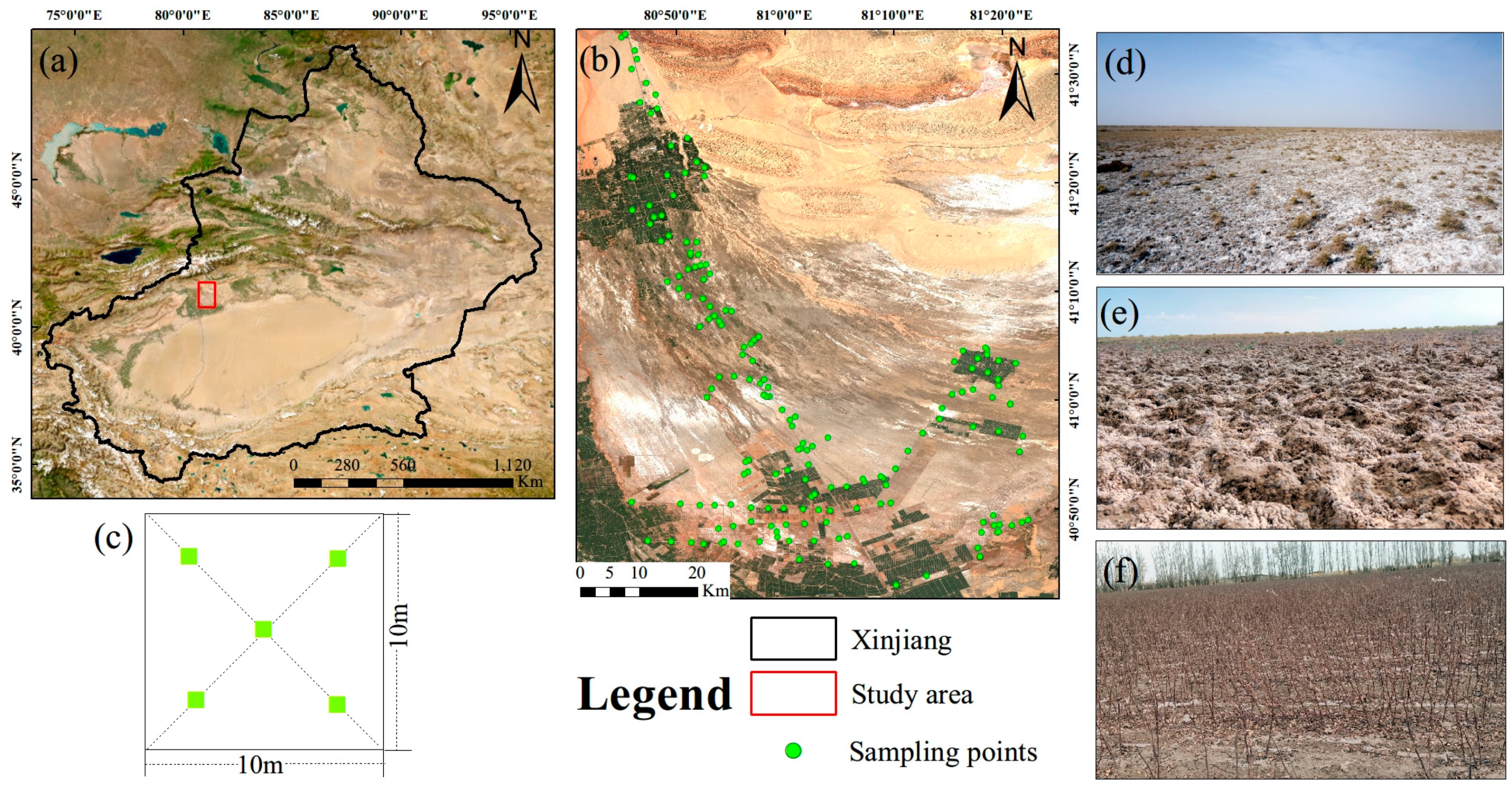
2.1. Study Area

The study area is located in Wensu County, Aksu Prefecture, at the northwestern boundary of the Taklamakan Desert in Southern Xinjiang, China. It extends from 80°40′ to 81°25′ E and 40°41′ to 13°34′ N (Figure 1). Situated deep in the Eurasian continent, the region has a temperate continental arid climate. Precipitation is minimal, while evaporation rates are high, with an evaporation-to-precipitation ratio nearing 30 [7]. The predominant soil types include saline soil and brown desert soil. The vegetation types mainly include natural species such as Halocnemum strobilaceum, Tamarix chinensis Lour, and Haloxylon ammodendron, as well as the salt-tolerant crop cotton. The roads in the study area mainly consist of one main north–south road and two secondary roads running east–west. In recent years, parts of the southern desert have been converted into cropland to address the rising food needs of a growing population. The continuous expansion of agricultural activities has profoundly impacted soil aggregate stability and SOC stocks, while also posing a threat to local agricultural resources and the ecological environment.

2.2. Soil Sample Collection and Preparation

To establish a ground observation dataset for SOC modeling, 170 topsoil samples were collected from the 0–20 cm layer along the main and secondary roads in November 2021. At each sampling site, five subsamples were gathered using the diagonal method within a 10 m × 10 m area. These subsamples were well mixed and processed using the quartering method to obtain a composite sample (500 g) [21]. Furthermore, the geographic coordinates at the center of each sampling site were documented utilizing a Juno SA PDA handheld GPS device. After laboratory pretreatment, the SOC was measured using the potassium dichromate oxidation method with external heating [21].

2.3. Data Collection and Analysis

2.3.1. Topographic Covariates

Topography is a crucial factor influencing soil formation and directly affecting the redistribution of matter and energy [23,32]. Therefore, topographic factors are often considered as the main environmental covariates in SOC mapping studies [17]. This study used Digital Elevation Model (DEM) data from the SRTM1 product with a resolution of 30 m supplied by the US Geological Survey, accessed via the GEE cloud platform (USGS/SRTMGL1_003). Based on the findings of previous studies, five topographic covariates that have significant impacts on SOC mapping were selected (Table 1) [13,15,23].

Using the cubic spline interpolation function in the ArcMap module of ArcGIS 10.8.1, these topographic variables were resampled to a 10 m resolution to align with the pixel size of the S-1 imagery.

2.3.2. S-1 Images

S-1, an integral part of the European Space Agency’s (ESA) Copernicus project, is a satellite designed for Earth observation, featuring C-band SAR. It provides various polarization settings, multiple imaging modes, high spatial resolution, and frequent revisit times [30]. For this study, images acquired from 2017 to 2021 in the vertical–vertical (VV) and vertical–horizontal (VH) polarization modes, functioning in interferometric wide (IW) beam mode, were selected for examination. Two S-1A images were needed to cover the entire study area, and the number of S-1A ascending and descending orbit images used in this study is presented in Figure 2.

The Ground Range Detected (GRD) products utilized in this study were sourced from S-1 imagery on the GEE platform and preprocessed using the ESA S-1 Toolbox. According to Mullissa et al. [33], S-1 GRD images have a pixel spacing of 10 m and a spatial resolution of 20 × 22 m. The preprocessing procedures involve orbit parameter adjustment, removal of GRD boundary noise, radiometric calibration, terrain correction, and thermal noise elimination [33]. These processing steps convert the dimensionless backscatter intensity into backscatter coefficients, which are quantified in decibels (dB). Due to the interference of electromagnetic radiation, radar images inevitably generate random speckle noise, but GEE’s preprocessing does not include filtering. We compare the Refined Lee, Boxcar, Frost and other filtering methods in SNAP software and select the optimal Refined Lee filtering method to be applied to GEE to remove the coherent speckle noise. Additionally, annual cumulative indices have been demonstrated to have a substantial positive impact on DSM in optical remote sensing [20]. Therefore, we also attempted to develop new S-1 annual cumulative indices for monitoring SOC.

We calculated a total of 24 S-1 indices, categorized into four types: (1) dual-polarization indices: VV, VH; (2) SAR vegetation indices: VVVHR, VHVVR, NDIVV, SSVI; (3) SAR texture indices: VV_ASM, VH_ASM, VV_Contrast, VH_Contrast, VV_Dissimilarity, VH_Dissimilarity, VV_Entropy, VH_Entropy, VV_Correlation, VH_Correlation, VV_Variance, VH_Variance; (4) SAR annual cumulative indices: VV-Max, VH-Max, VV-Min, VH-Min, VV-Mean, VH-Mean. Table 1 presents the detailed formulas for these indices.

Table 1. Variables used in this study for predicting SOC.

Variable Category	Predictor	Acronyms	Formula	Reference
Topographic variable	Elevation	DEM		[7]
	Aspect	AS
	Topographic Wetness Index	TWI
	Slope	S
	Topographic Roughness Index	TRI		[34]
Remote sensing variable	Vertically polarized backscatter	VV		[35]
	Horizontally polarized backscatter	VH
	VV-VH Cross-Polarization Ratio	VVVHR	$VV/VH$
	VH-VV Cross-Polarization Ratio	VHVVR	$VH/VV$
	Normalized Difference VV-VH Ratio	NDIVV	$\left(VV-VH\right)/\left(VV+VH\right)$
	SAR Sum Vegetation Index	SSVI	$VV+VH$	[36]
	GLCM Angular Second Moment from VV	VV_ASM	${\displaystyle \sum _{i=0}^{N-1}}{\displaystyle \sum _{j=0}^{N-1}}P{\left(i,j\right)}^2$	[29]
	GLCM Angular Second Moment from VH	VH_ASM
	GLCM Contrast from VV	VV_Contrast	${\displaystyle \sum _{i,j=0}^{N-1}}{iP}_{i,j}{\left(i-j\right)}^2$
	GLCM Contrast from VH	VH_Contrast
	GLCM Dissimilarity from VV	VV_Dissimilarity	${\displaystyle \sum _{i,j=0}^{N-1}}{iP}_{i,j}\left|i-j\right|$
	GLCM Dissimilarity from VH	VH_Dissimilarity
	GLCM Entropy from VV	VV_Entropy	${\displaystyle \sum _{i,j=0}^{N-1}}{iP}_{i,j}\left(-\ln P_{i,j}\right)$
	GLCM Entropy from VH	VH_Entropy
	GLCM Correlation from VV	VV_Correlation	${\displaystyle \sum _{i,j=0}^{N-1}}{iP}_{i,j}\left[{\displaystyle \frac{\left(i-mean\right)\left(j-mean\right)}{\sqrt{{var}_i\ast {var}_j}}}\right]$
	GLCM Correlation from VH	VH_Correlation
	GLCM Variance from VV	VV_Variance	${\displaystyle \sum _{i,j=0}^{N-1}}{iP}_{i,j}{(i-mean)}^2$
	GLCM Variance from VH	VH_Variance
	Annual Maximum VV Cumulative Index	VV-Max	$$\begin{gathered} {VV-Max}_{\left(x,y\right)} \\ ={\sum }_{t\in \left[1,T\right]}^{Max}{VV}_{\left(x,y\right)} \end{gathered}$$	this study
	Annual Maximum VH Cumulative Index	VH-Max	$$\begin{gathered} {VH-Max}_{\left(x,y\right)} \\ ={\sum }_{t\in \left[1,T\right]}^{Max}{VH}_{\left(x,y\right)} \end{gathered}$$
	Annual Minimum VV Cumulative Index	VV-Min	${VV-Min}_{\left(x,y\right)}={\sum }_{t\in \left[1,T\right]}^{Min}{VV}_{\left(x,y\right)}$
	Annual Minimum VH Cumulative Index	VH-Min	$$\begin{gathered} {VH-Min}_{\left(x,y\right)} \\ ={\sum }_{t\in \left[1,T\right]}^{Min}{VH}_{\left(x,y\right)} \end{gathered}$$
	Annual Mean VV Cumulative Index	VV-Mean	$$\begin{gathered} {VV-Mean}_{\left(x,y\right)} \\ ={\sum }_{t\in \left[1,T\right]}^{Mean}{VV}_{\left(x,y\right)} \end{gathered}$$
	Annual Mean VH Cumulative Index	VH-Mean	$$\begin{gathered} {VV-Max}_{\left(x,y\right)} \\ ={\sum }_{t\in \left[1,T\right]}^{Mean}{VV}_{\left(x,y\right)} \end{gathered}$$

Note: According to the formula above, N denotes the total number of grey levels, and P (i, j) indicates the normalized grey scale value at position (i, j), with i and j representing the respective grey levels. Additionally, x and y refer to the geographic coordinates of the pixel, while t signifies the time of image acquisition across the entire series, ranging from 1 to T (the final date).

Table 1. Variables used in this study for predicting SOC.

Variable Category	Predictor	Acronyms	Formula	Reference
Topographic variable	Elevation	DEM		[7]
	Aspect	AS
	Topographic Wetness Index	TWI
	Slope	S
	Topographic Roughness Index	TRI		[34]
Remote sensing variable	Vertically polarized backscatter	VV		[35]
	Horizontally polarized backscatter	VH
	VV-VH Cross-Polarization Ratio	VVVHR	$VV/VH$
	VH-VV Cross-Polarization Ratio	VHVVR	$VH/VV$
	Normalized Difference VV-VH Ratio	NDIVV	$\left(VV-VH\right)/\left(VV+VH\right)$
	SAR Sum Vegetation Index	SSVI	$VV+VH$	[36]
	GLCM Angular Second Moment from VV	VV_ASM	${\displaystyle \sum _{i=0}^{N-1}}{\displaystyle \sum _{j=0}^{N-1}}P{\left(i,j\right)}^2$	[29]
	GLCM Angular Second Moment from VH	VH_ASM
	GLCM Contrast from VV	VV_Contrast	${\displaystyle \sum _{i,j=0}^{N-1}}{iP}_{i,j}{\left(i-j\right)}^2$
	GLCM Contrast from VH	VH_Contrast
	GLCM Dissimilarity from VV	VV_Dissimilarity	${\displaystyle \sum _{i,j=0}^{N-1}}{iP}_{i,j}\left|i-j\right|$
	GLCM Dissimilarity from VH	VH_Dissimilarity
	GLCM Entropy from VV	VV_Entropy	${\displaystyle \sum _{i,j=0}^{N-1}}{iP}_{i,j}\left(-\ln P_{i,j}\right)$
	GLCM Entropy from VH	VH_Entropy
	GLCM Correlation from VV	VV_Correlation	${\displaystyle \sum _{i,j=0}^{N-1}}{iP}_{i,j}\left[{\displaystyle \frac{\left(i-mean\right)\left(j-mean\right)}{\sqrt{{var}_i\ast {var}_j}}}\right]$
	GLCM Correlation from VH	VH_Correlation
	GLCM Variance from VV	VV_Variance	${\displaystyle \sum _{i,j=0}^{N-1}}{iP}_{i,j}{(i-mean)}^2$
	GLCM Variance from VH	VH_Variance
	Annual Maximum VV Cumulative Index	VV-Max	$$\begin{gathered} {VV-Max}_{\left(x,y\right)} \\ ={\sum }_{t\in \left[1,T\right]}^{Max}{VV}_{\left(x,y\right)} \end{gathered}$$	this study
	Annual Maximum VH Cumulative Index	VH-Max	$$\begin{gathered} {VH-Max}_{\left(x,y\right)} \\ ={\sum }_{t\in \left[1,T\right]}^{Max}{VH}_{\left(x,y\right)} \end{gathered}$$
	Annual Minimum VV Cumulative Index	VV-Min	${VV-Min}_{\left(x,y\right)}={\sum }_{t\in \left[1,T\right]}^{Min}{VV}_{\left(x,y\right)}$
	Annual Minimum VH Cumulative Index	VH-Min	$$\begin{gathered} {VH-Min}_{\left(x,y\right)} \\ ={\sum }_{t\in \left[1,T\right]}^{Min}{VH}_{\left(x,y\right)} \end{gathered}$$
	Annual Mean VV Cumulative Index	VV-Mean	$$\begin{gathered} {VV-Mean}_{\left(x,y\right)} \\ ={\sum }_{t\in \left[1,T\right]}^{Mean}{VV}_{\left(x,y\right)} \end{gathered}$$
	Annual Mean VH Cumulative Index	VH-Mean	$$\begin{gathered} {VV-Max}_{\left(x,y\right)} \\ ={\sum }_{t\in \left[1,T\right]}^{Mean}{VV}_{\left(x,y\right)} \end{gathered}$$

Note: According to the formula above, N denotes the total number of grey levels, and P (i, j) indicates the normalized grey scale value at position (i, j), with i and j representing the respective grey levels. Additionally, x and y refer to the geographic coordinates of the pixel, while t signifies the time of image acquisition across the entire series, ranging from 1 to T (the final date).

This study introduced an innovative approach to analyzing time-series S-1 data. Initially, the correlation between soil properties and time-series data exhibited temporal fluctuations [37]. Correlation analysis was conducted to explore the temporal variation patterns between SOC and time-series S-1 data. At the monthly scale, the relationship between SOC and S-1 data exhibits significant shifts, indicating that annually, there exists a specific time point where the correlation between SOC and S-1 data reaches its peak. This time point was designated as the “optimal monitoring phase”. However, because of annual differences in plant phenology or variations in the rainy season’s timing, the optimal monitoring phase can vary between years. This range of variation was termed the “optimal monitoring period”. By determining the optimal monitoring period, we can eliminate irrelevant temporal features, thereby improving the efficiency of SOC monitoring.

2.4. Feature Selection Algorithm

Feature selection algorithms can identify the most relevant features and remove redundant variables [38]. As the multi-year S-1 optimal monitoring period data still retain relatively abundant temporal features, feature selection algorithms are essential for tackling this challenge [1]. This study evaluated three widely used feature selection algorithms to evaluate their potential for enhancing the construction of prediction models, namely recursive feature elimination (RFE), Boruta, ant colony optimization (ACO). RFE is a backward-selection algorithm [39]. The Boruta algorithm is a wrapper-based feature selection method [40]. ACO is a meta-heuristic algorithm inspired by the foraging behavior of ants [41]. The RFE algorithm and Boruta algorithm were implemented via the caret package and Boruta package in R Studio 2023.12.1 Build 402, respectively [40,42], while the ACO algorithm was executed in the MATLAB R2020a environment. The results show that the Boruta, RFE, and ACO algorithms selected 49, 40, and 45 feature variables from the original variables, respectively. In comparison to the original multi-year optimal monitoring period datasets (which included 1162 variables), feature selection reduced the number of variables by 95.79%, 96.56%, and 96.13%, effectively removing redundant covariates and significantly lowering both computational demands and model complexity.

2.5. Construction of SOC Prediction Models

Linear regression models have intuitive understanding and interpretation, while machine learning and deep learning models can effectively solve nonlinear problems [15]. This study systematically compares and analyzes different types of prediction models. including deep learning model CNN-LSTM, machine learning model RF and linear regression model PLSR. Figure 3 presents the detailed architecture of the CNN-LSTM model. The input time-series data first go through the CNN to extract spatial features, which are then learned by the LSTM. Following the learning process, the output from the LSTM layer is fed into the fully connected layer, which generates the final predicted value.

2.6. Model Assessment and Uncertainty

We employed 10-fold cross-validation to evaluate and compare the performance of the model. Three standard metrics—R², Relative Prediction Deviation (RPD), and Root Mean Square Error (RMSE)—were utilized to accurately measure the performance of different models. R² is appropriate for assessing the fit of regression models, while RMSE is used to evaluate the overall prediction accuracy. RPD measures how well the model explains the variability in the dependent variable. Beyond assessing model performance, quantifying prediction uncertainty is equally essential [30]. The reliability of the model’s outputs can be evaluated by computing the standard deviation (SD) of predictions generated through cross-validation [20]. The workflow of this study is illustrated in Figure 4.

3. Results

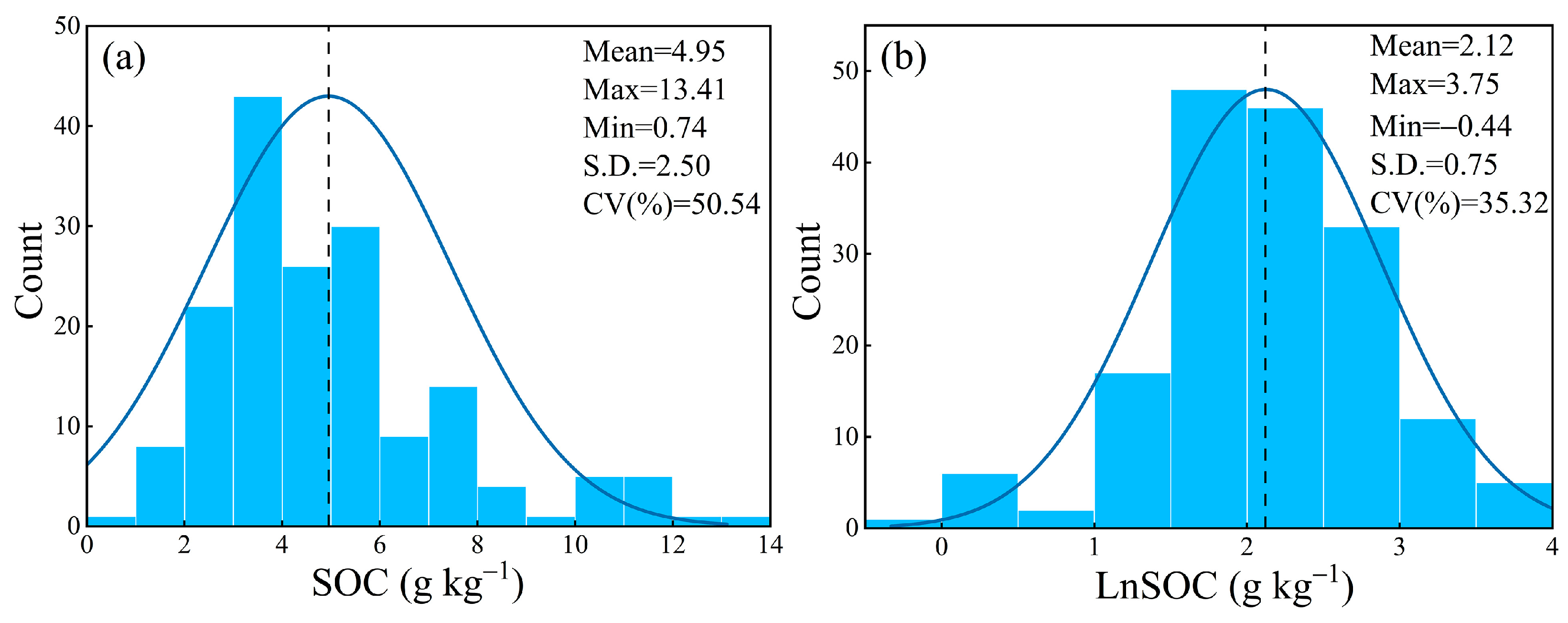
3.1. Summary Statistics of SOC

The summary statistics of SOC and logarithmically transformed SOC (LnSOC) for the 170 soil samples are displayed in Figure 5. The average SOC content was 4.95 g kg⁻¹, indicating an overall low content of SOC. SOC showed high variability (coefficient of variation at 50.54%), pointing to considerable spatial variability in its distribution throughout the region. Additionally, SOC data also exhibited a right-skewed distribution. The SOC data were subjected to a logarithmic transformation, resulting in LnSOC that approximates a normal distribution (Figure 5b), thereby improving the model’s stability and precision. After completing the predictive analysis, the SOC data were inversely transformed from log scale back to the original scale.

3.2. Correlation Analysis of Covariates with SOC

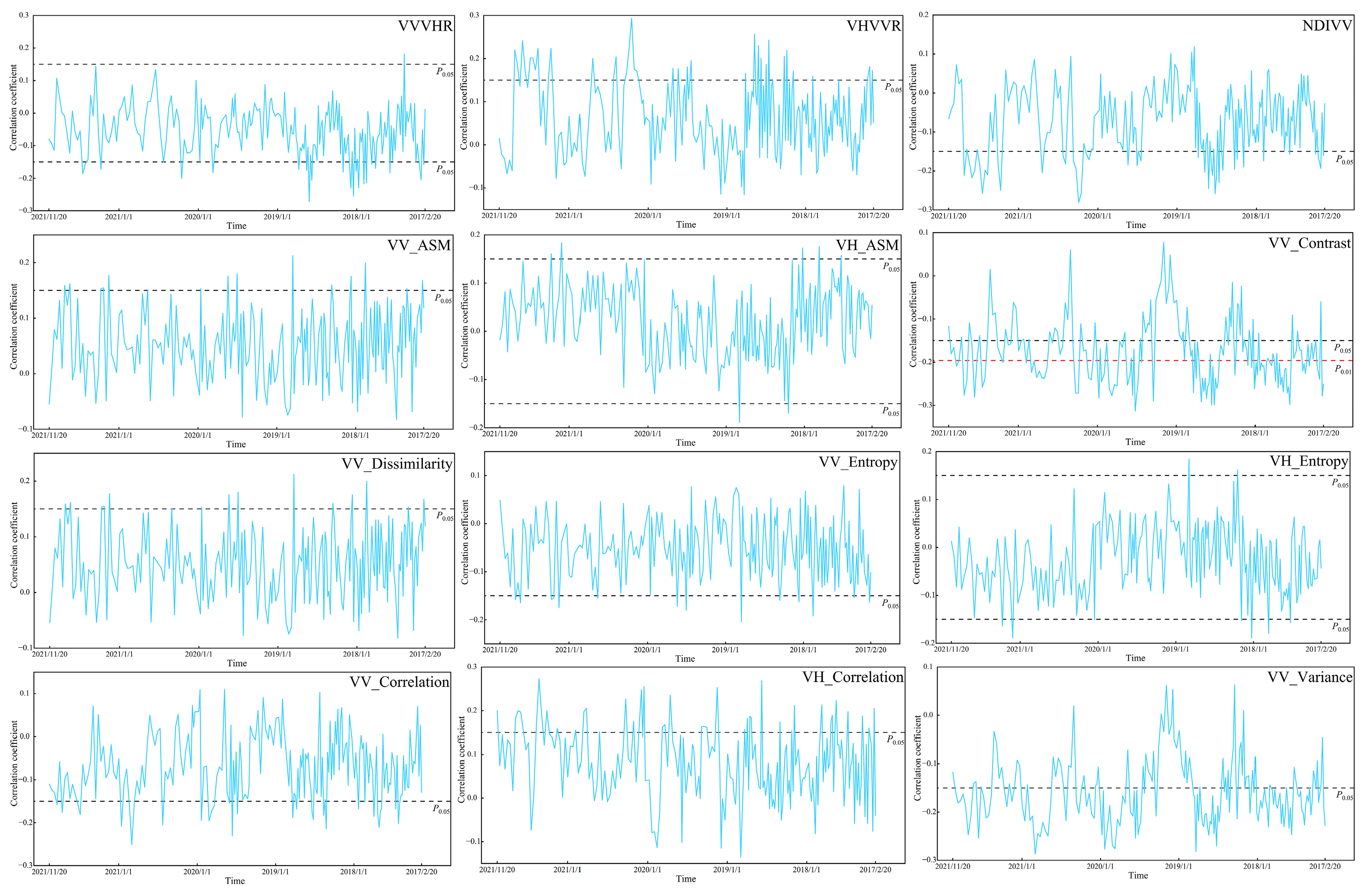
3.2.1. The Temporal Correlation Patterns Between SOC and Time-Series S-1 Data

The temporal variation pattern of the correlation between SOC and time-series S-1 data is shown in Figure 6 and Appendix A. As shown in Figure 6, the correlation observed between SOC and time-series S-1 data exhibited a cyclical pattern on an annual basis. The VV, VH, SSVI, VH_Contrast, VH_Dissimilarity, and VH_Variance initially increased and then decreased from January to April, followed by a rapid increase from May to June, a slow rise from July to September, and an initial decrease that then increased again from October to December. On the other hand, the correlation between SOC and other indices fluctuated over different months. Within the annual cycle, the time points were concentrated between July and October. Therefore, it was determined that the optimal monitoring period for using S-1 data to monitor SOC was from July to October. By identifying this optimal monitoring period, the data volume was reduced by 73.27% relative to the initial time-series dataset.

The correlation between SOC and time-series S-1 data displayed a decreasing trend based on annual variation patterns. Specifically, the correlation between SOC and VV, VH, SSVI, VHVVR, VH_Dissimilarity, VV_Correlation, VV_Variance, VH_Variance, VV_Contrast, VH_Contrast, and VH_Correlation decreased from an extremely significant level to a significant level by 2017. The correlation between SOC and NDIVV, VV_ASM, VH_ASM, VV_Dissimilarity, VV_Entropy, and VH_Entropy decreased from a significant level to a non-significant level by 2017.

By comparing the correlation between SOC and different indices, it was found that the VV, VH, and SSVI indices were positively correlated with SOC. In terms of texture features, the VH_Contrast, VH_Dissimilarity, and VH_Variance indices were negatively correlated with SOC, and they exhibited relatively high correlations with SOC. The highest correlation coefficients were 0.459, 0.587, 0.543, 0.443, 0.487, and 0.390. The correlations of other indices fluctuated between positive and negative values, and their correlations with SOC were not significant.

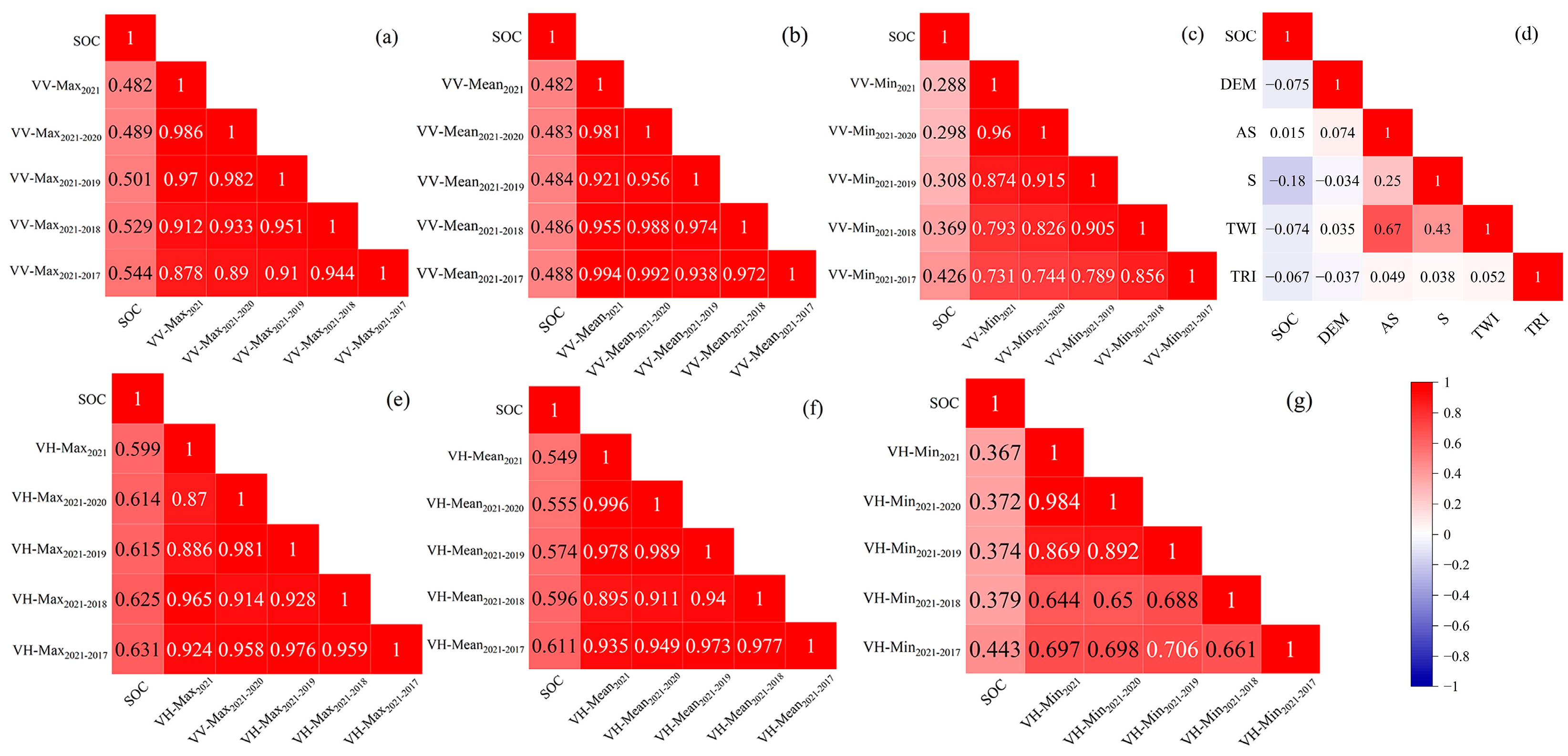
3.2.2. Correlation Analysis of SAR Annual Cumulative Indices and Topographic Covariates with SOC

The correlation between the six SAR annual cumulative indices and the five topographic covariates extracted using DEM with SOC is shown Figure 7. The correlation of VV and VH with SOC was significantly improved after the cumulative transformation of maximum and mean values, and the improvement was better with an increase in cumulative years. The improvement effect of the minimum annual accumulation on the correlation with SOC was not significant and was even less effective than VV and VH. Compared with the mean value accumulation, the maximum value accumulation showed better improvement effects. Between VV and VH, the VH accumulation showed a more significant improvement. Compared to the highest correlation coefficient of VV with SOC at 0.459, the maximum and mean value annual cumulative indices of VV showed higher correlation coefficients, exceeding by 0.023–0.085 and 0.023–0.029, respectively. Similarly, compared to the highest correlation coefficient of VH with SOC at 0.587, the maximum value annual cumulative index of VH showed a higher correlation coefficient, exceeding by 0.011–0.043. Therefore, constructing maximum or mean value cumulative indices can significantly improve the correlation between VV and VH with SOC.

The topographic covariates were negatively correlated to SOC and had quite low correlations, with only the slope reaching a significant level, while other topographic covariates were not significant (Figure 7d). Even though we considered topographic factors in relation to the spatial distribution of SOC, their effect was not significant due to the relatively small variation in topography across this region.

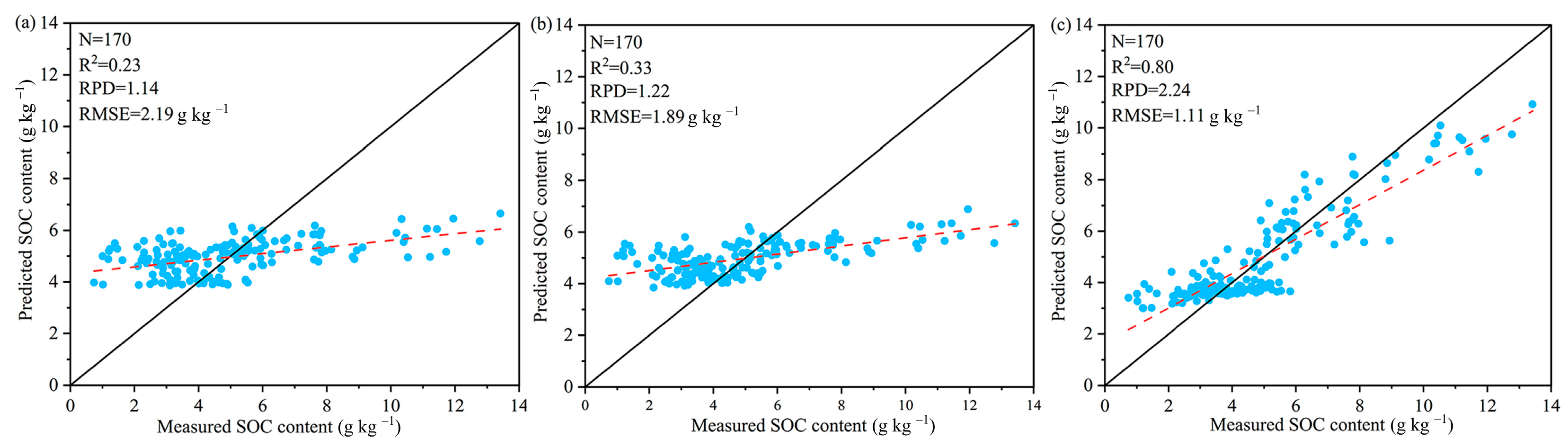
3.3. Evaluation and Comparison of Three Predictive Models

The comparative performance evaluation of the different inversion models formulated using four different datasets is presented in

Table 2. Comparison of accuracy for three SOC predictive models with different feature selection algorithms.

Model	Dataset	Training			Testing
		R2	RPD	RMSE	R2	RPD	RMSE
PLSR	All	0.41	1.30	2.06	0.28	1.18	2.10
	ACO	0.43	1.33	1.37	0.36	1.25	2.00
	RFE	0.44	1.34	1.89	0.38	1.27	1.76
	Boruta	0.46	1.36	1.88	0.39	1.28	1.92
RF	All	0.52	1.46	1.53	0.43	1.32	1.65
	ACO	0.70	1.83	1.37	0.56	1.51	1.64
	RFE	0.75	2.02	1.24	0.69	1.78	1.39
	Boruta	0.79	2.19	1.14	0.72	1.88	1.32
CNN-LSTM	All	0.59	1.57	1.50	0.51	1.43	1.52
	ACO	0.78	2.14	1.20	0.67	1.75	1.25
	RFE	0.81	2.28	1.10	0.73	1.93	1.33
	Boruta	0.85	2.54	0.99	0.80	2.24	1.11

. The results indicated that the choice of feature selection algorithms and modeling methods significantly impacted the modeling accuracy. Compared to the full dataset, the three feature selection algorithms improved the accuracy of predictive models to varying degrees, especially for the CNN-LSTM model, where the R² increased by 0.16–0.29. Among the various feature selection methods, Boruta performed the best in terms of dataset selection, while RFE and ACO ranked second and third, respectively. For model comparison, the accuracy of the deep learning, machine learning and linear regression models varied, with the CNN-LSTM model performing better, followed by RF and PLSR. Thus, Boruta outperformed RFE and ACO in feature selection, and among the models, the CNN-LSTM model surpassed both RF and PLSR in performance. Therefore, the Boruta algorithm is superior to RFE and ACO in feature selection, while among the models, the CNN-LSTM model achieved superior performance compared to both PLSR and RF. Ultimately, the CNN-LSTM model, built using the feature dataset selected by the Boruta algorithm, delivered the highest performance (R² = 0.80, RPD = 2.24, RMSE = 1.11 g kg⁻¹).

3.4. The Relative Variable Importance

Figure 8 illustrates the relative importance of variables in the optimal model. By normalizing the importance of all variables to a scale of 100%, we improved the comparability among them, providing a more precise representation of their contributions to the SOC prediction model. Among individual variables, VH-2021/8/28 had the highest relative importance (5.47%). In contrast, VH_Dissimilarity-2017/7/20 had the lowest relative importance (0.78%). For the same category of variables, dual-polarization indices were most important, with a relative importance of 49.83%. SAR vegetation indices came next, followed by SAR annual cumulative indices. SAR texture indices contributed the least, at 5.19%. Among the newly developed SAR annual cumulative indices, the VH maximum annual cumulative index and the VH mean annual cumulative index had a combined relative importance of 17.93%, validating the effectiveness of SAR annual cumulative indices. Additionally, the relative importance of SAR annual cumulative indices increased with the accumulation period. Within the dual-polarization indices, the VH index’s relative importance surpassed that of the VV index by 45.93% (total contribution rate of 49.83%). It showed that VH was more important for SOC modelling since it captured information on vegetation morphology and aboveground biomass. In contrast, the VV polarization was more sensitive to soil moisture content. This observation aligns with the findings of prior research [22,27,28]. Based on the variable distribution across different years, the majority of variables were concentrated around the years closest to the sampling period, particularly from 2018 to 2021, with a comparatively smaller number of feature factors selected from 2017.

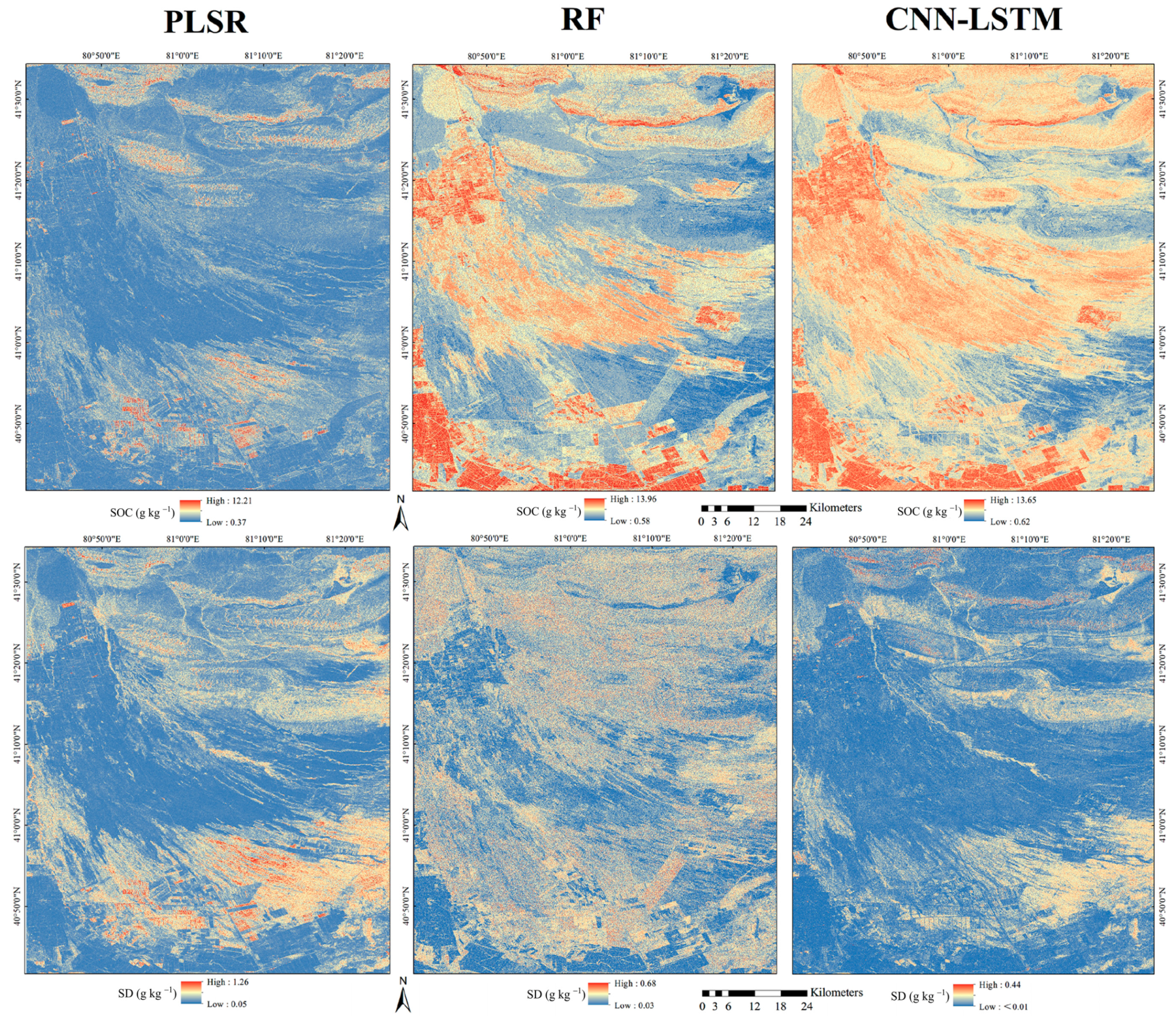
3.5. Spatial Distribution of SOC and Its Uncertainty

This study employed three predictive models constructed using variables selected by Boruta to map SOC. The resulting spatial distributions of SOC and their corresponding uncertainty maps, as derived from these three models, are shown in Figure 9. The spatial patterns of SOC derived from the RF and CNN-LSTM models were largely similar, whereas the SOC distribution produced by the PLSR model showed notable discrepancies when compared to the other two models. According to the map provided by RF and the CNN-LSTM model, the SOC showed strong spatial heterogeneity in the study area (Figure 9). Generally, higher SOC contents were found in long-term cultivated farmland, whereas lower SOC contents were observed in desert areas, mountainous regions, and newly cultivated farmland. Long-term cultivated farmland exhibits high SOC levels, primarily attributed to sustained fertilization practices and straw incorporation, which enhance SOC inputs. Conversely, desert and mountainous regions with sparse vegetation show low SOC due to limited organic matter sources. Newly cultivated farmland, situated in previously desert areas, has an inherently low SOC content. Additionally, the short cultivation history further restricts improvements in soil fertility. The mean SOC values of the PLSR, RF, and CNN-LSTM models were 4.57 g kg⁻¹, 5.52 g kg⁻¹, and 5.06 g kg⁻¹, respectively. Compared with the mean observed SOC value (4.95 g kg⁻¹), the PLSR model underestimated this value, while the RF model overestimated it. Among the three models, the SOC mean values and ranges from the CNN-LSTM model were the most comparable to the ground survey results, demonstrating its best performance in predicting SOC.

Regarding uncertainty, areas with elevated SOC uncertainty are predominantly found in the southeastern desert and northern mountainous regions, both of which are associated with low SOC levels (Figure 9). Conversely, regions with higher SOC content demonstrated significantly lower uncertainty. In comparison to the PLSR and RF models, the CNN-LSTM model mapped SOC with a lower uncertainty. As a result, the SOC spatial distribution map generated by the CNN-LSTM model demonstrated greater reliability and stability.

4. Discussion

4.1. Potential of Time-Series S-1 Data for Mapping SOC

The quantitative prediction of soil properties using remote sensing technology depends on the availability and quality of images [43,44]. The greatest advantage of S-1 microwave radar data over optical data is that they are not constrained by weather conditions and can provide continuous time-series images. However, many studies that focus on monitoring and mapping SOC using S-1 data have mostly relied on either single- or multi-date data. These studies, however, do not fully harness the potential of utilizing time-series S-1 data for more effective SOC monitoring.

The ability to predict SOC using soil–vegetation relationships depends on capturing vegetation characteristics that reflect SOC changes from remote sensing images [45]. Santos et al. [27] found an R² of only 0.24 when monitoring SOC using single-date S-1 dual-polarization SAR vegetation indices. Many studies have demonstrated that using multi-date S-1 data can improve SOC monitoring accuracy compared to single-date data [30,46]. For instance, Yang and Guo [22] successfully predicted the SOC content at three different depths using multi-date S-1 data (RPD = 1.22, RMSE = 1.63 g kg⁻¹). Similarly, we compared the performance of monitoring SOC using single- and multi-date data. The prediction accuracy for single- and multi-date data is illustrated in Figure 10, with R² values of 0.23 and 0.33, respectively. These results are consistent with existing studies on SOC monitoring using S-1 data [4,19,27,29,30], which report R² values ranging from 0.16 to 0.35, confirming the superiority of multi-date data over single-date data.

However, the SOC content is not only related to the vegetation information of the current year but also affected by the vegetation condition of the previous years. This is because SOC represents the humification and accumulation of plant residues in the soil over many years [42]. Therefore, long-term vegetation information has a more significant impact on SOC than single-year vegetation information [18]. Earlier research has shown that time-series remote sensing data offer advantages over both single- and multi-date data [47]. Time-series remote sensing imagery is effective in monitoring SOC because it can accurately capture the temporal fluctuations in vegetation, which directly influence the accumulation and decomposition of SOC [48]. Therefore, tracking vegetation changes in time-series remote sensing data can greatly enhance the accuracy of SOC monitoring. Zhang et al. [31] improved the precision of soil organic matter (SOM) prediction models using time-series Sentinel-2 data (R² increased by 10.4%). Zhang et al. [18] showed that incorporating long-term phenological variables significantly improved the accuracy of digital SOC mapping. Most previous studies have focused on optical remote sensing data for time-series analysis. However, since vegetation responds differently to backscatter coefficients at different growth stages, time-series S-1 data can also capture vegetation dynamic information. Consequently, we significantly improved the accuracy of SOC monitoring using time-series S-1 data. As shown in Figure 10, the modeling accuracy using time-series S-1 data is significantly better than using single-date data (R² = 0.23, RPD = 1.14, RMSE = 2.19 g kg⁻¹) and multi-date data (R² = 0.33, RPD = 1.22, RMSE = 1.89 g kg⁻¹), with the fit line of actual values and predicted values being closer to the 1:1 line. Specifically, the R² increased by 0.57 and 0.47, RPD increased by 1.10 and 1.02, while RMSE decreased by 1.08 g kg⁻¹ and 0.78 g kg⁻¹, respectively. This research greatly enhanced the accuracy of SOC monitoring with S-1 data, representing a crucial step forward in applying S-1 microwave radar data for SOC monitoring and mapping.

4.2. Optimal Monitoring Period for SOC Using S-1 Data

Many studies utilizing satellite remote sensing for SOC monitoring and mapping have predominantly employed single- or multi-date datasets, with prediction accuracy influenced by the selected time points [49]. The identification of the optimal monitoring period plays a key role in such studies, as it lays the groundwork for selecting appropriate remote sensing image timeframes and offers a valuable reference period for similar regions. Moreover, the optimal monitoring period for soil properties has also been explored in some studies. Luo et al. [38] conducted a comparative study on SOM prediction accuracy across different stages of the bare soil period. Their findings revealed that mid-May yielded the highest accuracy, thus establishing it as the optimal monitoring period for SOM in Northeast China. Luo et al. [47] used Landsat-8 median synthetic images to assess the accuracy of SOM prediction across different periods from April to October, finding that the highest accuracy was achieved during the April–June period. Previous research primarily focused on an annual scale, neglecting the inter-annual variability in the optimal monitoring period due to phenological changes. In comparison, this study aimed to establish the optimal monitoring period for SOC through a systematic evaluation of multi-year temporal patterns, thereby achieving enhanced detection of both cyclical seasonal changes and long-term annual SOC variations.

The optimal monitoring period for SOC in the arid Southern Xinjiang region of China using S-1 data is found to be from July to October. This is mainly attributable to the timing of this period within the wet season and the vegetation growth phase in the study area. Firstly, during the wet season, precipitation increases significantly, resulting in a notable rise in soil moisture levels. SOC is strongly associated with the soil’s ability to retain water [23]. S-1 data can accurately capture the spatial distribution of SOC during the wet season by tracking changes in soil moisture [50]. Secondly, diverse plant species experience distinct phenological phases during their peak growth seasons, which coincide with periods of maximum biomass and vigorous growth in the study area. Given the critical role of SOC in plant development, S-1 imagery effectively captures canopy characteristics during these peak vegetation phases, thereby supporting SOC monitoring efforts [51]. The optimal monitoring period for SOC, determined through S-1 data, not only optimizes the utilization of time-series S-1 data but also offers a useful reference period for comparable regions, improving the efficiency of SOC monitoring practices.

4.3. Prediction Performance of Different Models for SOC

Traditionally, linear models have long been used as baseline models, offering a crucial reference point for assessing the performance of alternative models [15]. Shi et al. [44] used Sentinel-2 multi-date data and the PLSR model to create high-resolution SOC distribution maps for farmland. Tripathi et al. [25] found that the ordinary least squares regression model performed well when using soil physicochemical properties and S-1 data to construct SOC prediction models. However, the intricate relationship between SOC and remote sensing and environmental factors is often non-proportional and non-monotonic, making nonlinear techniques more suitable for SOC monitoring [52]. The RF model, a conventional machine learning approach, is widely applied in DSM [17]. Zhang et al. [51] utilized the RF model to examine the spatial patterns of SOC across China and its sensitivity to future climate changes. The RF model is often chosen as a comparison model for complex models because of its excellent performance in most cases.

Deep learning models, in comparison to linear regression and machine learning models, provide substantial benefits in data analysis by uncovering complex spatial relationships and identifying key features within datasets [16]. Additionally, deep learning models can automatically extract stable and high-level abstract features from remote sensing data, thereby enhancing model performance. Our findings suggest that deep learning models provide superior performance compared to machine learning and linear regression models, aligning with the conclusions of prior research [20]. Two prevalent deep learning models extensively utilized in DSM are CNN and the LSTM, excelling in handling spatial and temporal data, respectively. Moreover, hybrid deep learning models combine the strengths of different deep learning models, enhancing mapping accuracy and detail [17]. The CNN-LSTM model integrates the feature extraction capabilities of CNN with the temporal modeling capabilities of LSTM, overcoming the limitations of individual models in processing sequential data and significantly improving the ability to handle time-series data. In our study, the CNN-LSTM model demonstrated superior performance on the optimal feature dataset, with R² and RMSE values on the test set improving by 0.41 and 0.04 and reducing by 0.81 g kg⁻¹ and 0.06 g kg⁻¹ compared to the PLSR and RF models, respectively. This is consistent with [18], where the CNN-LSTM model outperformed the RF model and confirmed the feasibility and potential of the CNN-LSTM model in DSM, especially in mining time-series remote sensing data.

4.4. Uncertainty Analysis

Uncertainty is inevitable in DSM [20]. In this study, limited access to the northern mountainous region and southeastern desert area resulted in insufficient sampling points, which contributed to greater uncertainty in these areas. In this case, the use of uncertainty information can guide supplementary soil sampling points to enhance the precision of SOC mapping [48]. In addition, SOC displays significant spatial variability, with its concentration and turnover rate primarily driven by various factors, resulting in complex and uncertain spatial distribution characteristics of SOC [53]. Moreover, different natural conditions, land use types, degrees of human disturbance, and soil properties influence the input of SOC and the microbial decomposition and transformation of SOC, thereby affecting its content [48,52]. For digital SOC mapping, it is necessary to comprehensively consider various variables representing heterogeneity factors while also accounting for the scale effect of SOC [16]. Additionally, the S-1 backscatter coefficient is influenced by numerous ground interference factors. The interaction between S-1 SAR incident electromagnetic waves and the ground surface is related not only to SAR system parameters but also to the soil dielectric constant, surface roughness, surface vegetation cover, and soil moisture. These factors affect both VV and VH polarized backscatter coefficients [30]. Ultimately, they impact the accuracy of digital SOC mapping. Despite the above uncertainties, we constructed a high-accuracy SOC predictive model with relatively low uncertainty, since this study fully exploited the potential of time-series S-1 data and leveraged the CNN-LSTM hybrid model.

Future studies could delve into the potential of utilizing time-series multi-source remote sensing data (such as S-1/2) for monitoring SOC. Meanwhile, efforts should be made to actively search for the optimal monitoring period for the remote sensing monitoring of different soil properties in other regions. It is expected to further enhance the efficiency and accuracy of DSM, providing more reliable data support for soil resource management and ecological environment research.

5. Conclusions

As far as we are aware, this is the first effort to investigate the potential of time-series S-1 data for digital SOC mapping, which was effectively implemented in the arid region of Southern Xinjiang, China. Our findings indicated that the combination of the optimal monitoring period and the feature selection approach for time-series data led to a substantial reduction in data dimensions. In contrast to the original dataset containing 3671 variables, the variables selected using the Boruta, RFE, and ACO methods reduced the number of variables by 98.67%, 98.91%, and 98.77%, respectively. This significantly reduced the data volume and improved the model accuracy. The predictive model constructed using time-series S-1 data exhibited significantly higher accuracy than models using single- and multi-date data. The CNN-LSTM model had the best performance (R² = 0.80, RPD = 2.24, RMSE = 1.11 g kg⁻¹). This represents a breakthrough in improving the mapping accuracy of SOC using time-series S-1 data compared to existing studies using single- or multi-date S-1 data. The newly developed annual accumulation indices of the VH maximum and mean significantly improved the correlation between SOC and S-1 data, contributing 17.93% to the best prediction model. This study highlights the considerable potential of time-series S-1 data for SOC monitoring and presents a fresh perspective on leveraging time-series remote sensing images for DSM.

References

1. Hu, B.; Xie, M.; Shi, Z.; Li, H.; Chen, S.; Wang, Z.; Zhou, Y.; Ni, H.; Geng, Y.; Zhu, Q.; et al. Fine-Resolution Mapping of Cropland Topsoil PH of Southern China and Its Environmental Application. Geoderma 2024, 442, 116798. [Google Scholar] [CrossRef]
2. Odebiri, O.; Mutanga, O.; Odindi, J.; Naicker, R. Modelling Soil Organic Carbon Stock Distribution across Different Land-Uses in South Africa: A Remote Sensing and Deep Learning Approach. ISPRS J. Photogramm. Remote Sens. 2022, 188, 351–362. [Google Scholar] [CrossRef]
3. Chen, Z.; Xue, J.; Wang, Z.; Zhou, Y.; Deng, X.; Liu, F.; Song, X.; Zhang, G.; Su, Y.; Zhu, P.; et al. Ensemble Modelling-Based Pedotransfer Functions for Predicting Soil Bulk Density in China. Geoderma 2024, 448, 116969. [Google Scholar] [CrossRef]
4. Zhou, T.; Geng, Y.; Chen, J.; Liu, M.; Haase, D.; Lausch, A. Mapping Soil Organic Carbon Content Using Multi-Source Remote Sensing Variables in the Heihe River Basin in China. Ecol. Indic. 2020, 114, 106288. [Google Scholar] [CrossRef]
5. Sun, Y.; Ma, J.; Zhao, W.; Qu, Y.; Gou, Z.; Chen, H.; Tian, Y.; Wu, F. Digital Mapping of Soil Organic Carbon Density in China Using an Ensemble Model. Environ. Res. 2023, 231, 116131. [Google Scholar] [CrossRef] [PubMed]
6. Díaz-Martínez, P.; Maestre, F.T.; Moreno-Jiménez, E.; Delgado-Baquerizo, M.; Eldridge, D.J.; Saiz, H.; Gross, N.; Le Bagousse-Pinguet, Y.; Gozalo, B.; Ochoa, V.; et al. Vulnerability of Mineral-Associated Soil Organic Carbon to Climate across Global Drylands. Nat. Clim. Change 2024, 14, 976–982. [Google Scholar] [CrossRef]
7. Peng, J.; Biswas, A.; Jiang, Q.; Zhao, R.; Hu, J.; Hu, B.; Shi, Z. Estimating Soil Salinity from Remote Sensing and Terrain Data in Southern Xinjiang Province, China. Geoderma 2019, 337, 1309–1319. [Google Scholar] [CrossRef]
8. Ren, Z.; Li, C.; Fu, B.; Wang, S.; Stringer, L.C. Effects of Aridification on Soil Total Carbon Pools in China’s Drylands. Glob. Change Biol. 2023, 30, e17091. [Google Scholar] [CrossRef]
9. Zhao, M.; Cao, G.; Zhao, Q.; Ma, Y.; Zhang, F.; Li, H.; He, Q.; Qiu, X. Distribution Patterns and Influencing Factors Controlling Soil Carbon in the Heihe River Source Basin, Northeast Qinghai–Tibet Plateau. Land 2025, 14, 409. [Google Scholar] [CrossRef]
10. De Benedetto, D.; Barca, E.; Castellini, M.; Popolizio, S.; Lacolla, G.; Stellacci, A.M. Prediction of Soil Organic Carbon at Field Scale by Regression Kriging and Multivariate Adaptive Regression Splines Using Geophysical Covariates. Land 2022, 11, 381. [Google Scholar] [CrossRef]
11. Chen, S.; Chen, Z.; Zhang, X.; Luo, Z.; Schillaci, C.; Arrouays, D.; Richer-De-Forges, A.C.; Shi, Z. European Topsoil Bulk Density and Organic Carbon Stock Database (0-20 Cm) Using Machine-Learning-Based Pedotransfer Functions. Earth Syst. Sci. Data 2024, 16, 2367–2383. [Google Scholar] [CrossRef]
12. Salgado, L.; González, L.M.; Gallego, J.L.R.; López-Sánchez, C.A.; Colina, A.; Forján, R. Mapping Soil Organic Carbon in Degraded Ecosystems Through Upscaled Multispectral Unmanned Aerial Vehicle–Satellite Imagery. Land 2025, 14, 377. [Google Scholar] [CrossRef]
13. Chen, S.; Arrouays, D.; Leatitia Mulder, V.; Poggio, L.; Minasny, B.; Roudier, P.; Libohova, Z.; Lagacherie, P.; Shi, Z.; Hannam, J.; et al. Digital Mapping of GlobalSoilMap Soil Properties at a Broad Scale: A Review. Geoderma 2022, 409, 115567. [Google Scholar] [CrossRef]
14. Zolfaghari Nia, M.; Moradi, M.; Moradi, G.; Taghizadeh-Mehrjardi, R. Machine Learning Models for Prediction of Soil Properties in the Riparian Forests. Land 2023, 12, 32. [Google Scholar] [CrossRef]
15. Lamichhane, S.; Kumar, L.; Wilson, B. Digital Soil Mapping Algorithms and Covariates for Soil Organic Carbon Mapping and Their Implications: A Review. Geoderma 2019, 352, 395–413. [Google Scholar] [CrossRef]
16. Odebiri, O.; Mutanga, O.; Odindi, J. Deep Learning-Based National Scale Soil Organic Carbon Mapping with Sentinel-3 Data. Geoderma 2022, 411, 115695. [Google Scholar] [CrossRef]
17. Pouladi, N.; Gholizadeh, A.; Khosravi, V.; Borůvka, L. Digital Mapping of Soil Organic Carbon Using Remote Sensing Data: A Systematic Review. Catena 2023, 232, 107409. [Google Scholar] [CrossRef]
18. Zhang, L.; Cai, Y.; Huang, H.; Li, A.; Yang, L.; Zhou, C. A CNN-LSTM Model for Soil Organic Carbon Content Prediction with Long Time Series of MODIS-Based Phenological Variables. Remote Sens. 2022, 14, 4441. [Google Scholar] [CrossRef]
19. Li, Z.; Liu, F.; Peng, X.; Hu, B.; Song, X. Synergetic Use of DEM Derivatives, Sentinel-1 and Sentinel-2 Data for Mapping Soil Properties of a Sloped Cropland Based on a Two-Step Ensemble Learning Method. Sci. Total Environ. 2023, 866, 161421. [Google Scholar] [CrossRef]
20. Wang, J.; Feng, C.; Hu, B.; Chen, S.; Hong, Y.; Arrouays, D.; Peng, J.; Shi, Z. A Novel Framework for Improving Soil Organic Matter Prediction Accuracy in Cropland by Integrating Soil, Vegetation and Human Activity Information. Sci. Total Environ. 2023, 903, 166112. [Google Scholar] [CrossRef]
21. Zhou, T.; Lv, W.; Geng, Y.; Xiao, S.; Chen, J.; Xu, X.; Pan, J.; Si, B.; Lausch, A. National-Scale Spatial Prediction of Soil Organic Carbon and Total Nitrogen Using Long-Term Optical and Microwave Satellite Observations in Google Earth Engine. Comput. Electron. Agric. 2023, 210, 107928. [Google Scholar] [CrossRef]
22. Yang, R.M.; Guo, W.W. Modelling of Soil Organic Carbon and Bulk Density in Invaded Coastal Wetlands Using Sentinel-1 Imagery. Int. J. Appl. Earth Obs. Geoinf. 2019, 82, 101906. [Google Scholar] [CrossRef]
23. Luo, C.; Zhang, W.; Zhang, X.; Liu, H. Mapping the Soil Organic Matter Content in a Typical Black-Soil Area Using Optical Data, Radar Data and Environmental Covariates. Soil Tillage Res. 2024, 235, 105912. [Google Scholar] [CrossRef]
24. Kunkel, V.R.; Wells, T.; Hancock, G.R. Modelling Soil Organic Carbon Using Vegetation Indices across Large Catchments in Eastern Australia. Sci. Total Environ. 2022, 817, 152690. [Google Scholar] [CrossRef] [PubMed]
25. Tripathi, A.; Tiwari, R.K. Utilisation of Spaceborne C-Band Dual Pol Sentinel-1 SAR Data for Simplified Regression-Based Soil Organic Carbon Estimation in Rupnagar, Punjab, India. Adv. Space Res. 2022, 69, 1786–1798. [Google Scholar] [CrossRef]
26. Ali, M.; Budillon, A.; Afzal, Z.; Schirinzi, G.; Hussain, S. PSInSAR-Based Time-Series Coastal Deformation Estimation Using Sentinel-1 Data. Land 2025, 14, 536. [Google Scholar] [CrossRef]
27. dos Santos, E.P.; Moreira, M.C.; Fernandes-Filho, E.I.; Demattê, J.A.M.; Dionizio, E.A.; Silva, D.D.d.; Cruz, R.R.P.; Moura-Bueno, J.M.; Santos, U.J.d.; Costa, M.H. Sentinel-1 Imagery Used for Estimation of Soil Organic Carbon by Dual-Polarization SAR Vegetation Indices. Remote Sens. 2023, 15, 5464. [Google Scholar] [CrossRef]
28. Wang, H.; Zhang, X.; Wu, W.; Liu, H. Prediction of Soil Organic Carbon under Different Land Use Types Using Sentinel-1/-2 Data in a Small Watershed. Remote Sens. 2021, 13, 1229. [Google Scholar] [CrossRef]
29. Nguyen, T.T.; Pham, T.D.; Nguyen, C.T.; Delfos, J.; Archibald, R.; Dang, K.B.; Hoang, N.B.; Guo, W.; Ngo, H.H. A Novel Intelligence Approach Based Active and Ensemble Learning for Agricultural Soil Organic Carbon Prediction Using Multispectral and SAR Data Fusion. Sci. Total Environ. 2022, 804, 150187. [Google Scholar] [CrossRef]
30. Zhou, T.; Geng, Y.; Lv, W.; Xiao, S.; Zhang, P.; Xu, X.; Chen, J.; Wu, Z.; Pan, J.; Si, B.; et al. Effects of Optical and Radar Satellite Observations within Google Earth Engine on Soil Organic Carbon Prediction Models in Spain. J. Environ. Manag. 2023, 338, 117810. [Google Scholar] [CrossRef]
31. Zhang, X.; Xue, J.; Chen, S.; Zhuo, Z.; Wang, Z.; Chen, X.; Xiao, Y.; Shi, Z. Improving Model Performance in Mapping Cropland Soil Organic Matter Using Time-Series Remote Sensing Data. J. Integr. Agric. 2024, 23, 2820–2841. [Google Scholar] [CrossRef]
32. Hu, B.; Ni, H.; Xie, M.; Li, H.; Wen, Y.; Chen, S.; Zhou, Y.; Teng, H.; Bourennane, H.; Shi, Z. Mapping Soil Organic Matter and Identifying Potential Controls in the Farmland of Southern China: Integration of Multi-Source Data, Machine Learning and Geostatistics. Land Degrad. Dev. 2023, 34, 5468–5485. [Google Scholar] [CrossRef]
33. Mullissa, A.; Vollrath, A.; Odongo-Braun, C.; Slagter, B.; Balling, J.; Gou, Y.; Gorelick, N.; Reiche, J. Sentinel-1 SAR Backscatter Analysis Ready Data Preparation in Google Earth Engine. Remote Sens. 2021, 13, 1954. [Google Scholar] [CrossRef]
34. Taghizadeh-Mehrjardi, R.; Schmidt, K.; Amirian-Chakan, A.; Rentschler, T.; Zeraatpisheh, M.; Sarmadian, F.; Valavi, R.; Davatgar, N.; Behrens, T.; Scholten, T. Improving the Spatial Prediction of Soil Organic Carbon Content in Two Contrasting Climatic Regions by Stacking Machine Learning Models and Rescanning Covariate Space. Remote Sens. 2020, 12, 1095. [Google Scholar] [CrossRef]
35. Schulz, C.; Förster, M.; Vulova, S.V.; Rocha, A.D.; Kleinschmit, B. Spectral-Temporal Traits in Sentinel-1 C-Band SAR and Sentinel-2 Multispectral Remote Sensing Time Series for 61 Tree Species in Central Europe. Remote Sens. Environ. 2024, 307, 114162. [Google Scholar] [CrossRef]
36. Mastro, P.; De Peppo, M.; Crema, A.; Boschetti, M.; Pepe, A. Statistical Characterization and Exploitation of Synthetic Aperture Radar Vegetation Indexes for the Generation of Leaf Area Index Time Series. Int. J. Appl. Earth Obs. Geoinf. 2023, 124, 103498. [Google Scholar] [CrossRef]
37. Zhang, T.T.; Qi, J.G.; Gao, Y.; Ouyang, Z.T.; Zeng, S.L.; Zhao, B. Detecting Soil Salinity with MODIS Time Series VI Data. Ecol. Indic. 2015, 52, 480–489. [Google Scholar] [CrossRef]
38. Luo, C.; Zhang, X.; Wang, Y.; Men, Z.; Liu, H. Regional Soil Organic Matter Mapping Models Based on the Optimal Time Window, Feature Selection Algorithm and Google Earth Engine. Soil Tillage Res. 2022, 219, 105325. [Google Scholar] [CrossRef]
39. Elith, J.; Leathwick, J.R.; Hastie, T. A Working Guide to Boosted Regression Trees. J. Anim. Ecol. 2008, 77, 802–813. [Google Scholar] [CrossRef]
40. Kursa, M.B.; Rudnicki, W.R. Feature Selection with the Boruta Package. J. Stat. Softw. 2010, 36, 1–13. [Google Scholar] [CrossRef]
41. Starzec, G.; Starzec, M.; Rutkowski, L.; Kisiel-Dorohinicki, M.; Byrski, A. Ant Colony Optimization Using Two-Dimensional Pheromone for Single-Objective Transport Problems. J. Comput. Sci. 2024, 79, 102308. [Google Scholar] [CrossRef]
42. Hu, B.; Xie, M.; Zhou, Y.; Chen, S.; Zhou, Y.; Ni, H.; Peng, J.; Ji, W.; Hong, Y.; Li, H.; et al. A High-Resolution Map of Soil Organic Carbon in Cropland of Southern China. Catena 2024, 237, 107813. [Google Scholar] [CrossRef]
43. Zhou, Y.; Chen, S.; Hu, B.; Ji, W.; Li, S.; Hong, Y.; Xu, H.; Wang, N.; Xue, J.; Zhang, X.; et al. Global Soil Salinity Prediction by Open Soil Vis-NIR Spectral Library. Remote Sens. 2022, 14, 5627. [Google Scholar] [CrossRef]
44. Shi, P.; Six, J.; Sila, A.; Vanlauwe, B.; Van Oost, K. Towards Spatially Continuous Mapping of Soil Organic Carbon in Croplands Using Multitemporal Sentinel-2 Remote Sensing. ISPRS J. Photogramm. Remote Sens. 2022, 193, 187–199. [Google Scholar] [CrossRef]
45. Yang, R.M.; Guo, W.W.; Zheng, J.B. Soil Prediction for Coastal Wetlands Following Spartina Alterniflora Invasion Using Sentinel-1 Imagery and Structural Equation Modeling. Catena 2019, 173, 465–470. [Google Scholar] [CrossRef]
46. Shafizadeh-Moghadam, H.; Minaei, F.; Talebi-khiyavi, H.; Xu, T.; Homaee, M. Synergetic Use of Multi-Temporal Sentinel-1, Sentinel-2, NDVI, and Topographic Factors for Estimating Soil Organic Carbon. Catena 2022, 212, 106077. [Google Scholar] [CrossRef]
47. Luo, C.; Zhang, W.; Zhang, X.; Liu, H. Mapping of Soil Organic Matter in a Typical Black Soil Area Using Landsat-8 Synthetic Images at Different Time Periods. Catena 2023, 231, 107336. [Google Scholar] [CrossRef]
48. Yang, C.; Yang, L.; Zhang, L.; Zhou, C. Soil Organic Matter Mapping Using INLA-SPDE with Remote Sensing Based Soil Moisture Indices and Fourier Transforms Decomposed Variables. Geoderma 2023, 437, 116571. [Google Scholar] [CrossRef]
49. Castaldi, F.; Halil Koparan, M.; Wetterlind, J.; Žydelis, R.; Vinci, I.; Özge Savaş, A.; Kıvrak, C.; Tunçay, T.; Volungevičius, J.; Obber, S.; et al. Assessing the Capability of Sentinel-2 Time-Series to Estimate Soil Organic Carbon and Clay Content at Local Scale in Croplands. ISPRS J. Photogramm. Remote Sens. 2023, 199, 40–60. [Google Scholar] [CrossRef]
50. Odebiri, O.; Mutanga, O.; Odindi, J.; Slotow, R.; Mafongoya, P.; Lottering, R.; Naicker, R.; Matongera, T.N.; Mngadi, M. Mapping Sub-Surface Distribution of Soil Organic Carbon Stocks in South Africa’s Arid and Semi-Arid Landscapes: Implications for Land Management and Climate Change Mitigation. Geoderma Reg. 2024, 37, e00817. [Google Scholar] [CrossRef]
51. Zhang, M.W.; Wang, X.Q.; Ding, X.G.; Yang, H.L.; Guo, Q.; Zeng, L.T.; Cui, Y.P.; Sun, X.L. Monitoring Regional Soil Organic Matter Content Using a Spatiotemporal Model with Time-Series Synthetic Landsat Images. Geoderma Reg. 2023, 34, e00702. [Google Scholar] [CrossRef]
52. Nieto, L.; Houborg, R.; Tivet, F.; Olson, B.J.S.C.; Prasad, P.V.V.; Ciampitti, I.A. Limitations and Future Perspectives for Satellite-Based Soil Carbon Monitoring. Environ. Chall. 2024, 14, 100839. [Google Scholar] [CrossRef]
53. Dai, W.; Huang, Y. Relation of Soil Organic Matter Concentration to Climate and Altitude in Zonal Soils of China. Catena 2006, 65, 87–94. [Google Scholar] [CrossRef]
Figure 1. Overview of the study area: (a) location of the study area; (b) distribution of soil sampling points; (c) five-point soil sampling; (d) desert region; (e) salt soil; (f) cotton field.
Land 14 00677 g001
Figure 2. Distribution of the number of S-1A ascending and descending images from 2017 to 2021 in the study area.
Land 14 00677 g002
Figure 3. Structure of the CNN-LSTM model used for SOC prediction.
Land 14 00677 g003
Figure 4. Schematic diagram of the SOC prediction process.
Land 14 00677 g004
Figure 5. Distributions of SOC content: original (a) and log-transformed (b). Note: S.D.: standard deviation; CV: coefficient of variation.
Land 14 00677 g005
Figure 6. The correlation patterns between time-series S-1 data and SOC. The black solid line represents the correlation coefficient at a significant level (P0.05 = 0.196), while the red solid line corresponds to the correlation coefficient at a highly significant level (P0.01 = 0.150). Note: vertical–vertical (VV); vertical–horizontal (VH).
Land 14 00677 g006
Figure 7. Heatmaps of the correlation between SAR annual cumulative index and topographic covariates with SOC. (ac) represent the correlations between the annual cumulative indices of the maximum value, the average value, and the minimum value of VV, respectively, and SOC. (d) represents the correlation between topographic factors and SOC. (eg) represent the correlations between the annual cumulative indices of the maximum value, the average value, and the minimum value of VH, respectively, and SOC.
Land 14 00677 g007
Figure 8. Variable importance in CNN-LSTM model with variables selected by Boruta.
Land 14 00677 g008
Figure 9. The predicted spatial distribution of SOC (g kg⁻1) with uncertainty assessment from three models.
Land 14 00677 g009
Figure 10. The values predicted by the models and the actual values for single-date data (a), multi-date data (b), and time-series data (c) derived from S-1.
Land 14 00677 g010