Abstract
The Mediterranean Diet is a highly sustainable diet, and legumes are among the products that best characterize this concept. This study evaluates the environmental sustainability of the Protected Geographical Indication (PGI) legume Phaseolus vulgaris L. cultivated in the Asturias region, Spain. Employing a multi-indicator approach, the study aims to define and measure certain biodiversity indicators useful for assessing the ecological quality and sustainability of the agroecosystems under consideration. Spatial analyses were conducted with GIS-based methodologies, integrating the Analytic Hierarchy Process (AHP) to generate a Sustainability Index (SI). The study found that a significant positive spatial autocorrelation was observed using Moran’s I test (Moran’s I = 0.74555, p < 0.01), indicating that the SI values were not equally distributed but clustered around particular regions. Furthermore, the Getis-Ord Gi* analysis determined statistically significant hotspots, mainly distributed in the western and southwestern areas, including regions near Cangas del Narcea and Tineo. This paper highlights the importance of integrating spatial analysis for environmental assessments to develop sustainability approaches. Soil quality, water use, biodiversity, and land management are some of the factors that affect sustainability outcomes in the region. The results underscore the role of PGI in promoting sustainable agricultural practices by meeting geographical and quality requirements for local production.
1. Introduction
The Mediterranean Diet is widely regarded as one of the healthiest eating models and among the most sustainable [1,2,3,4]. To preserve traditions related to food and traditional medicine, UNESCO has recognised its cultural, health, and environmental sustainability significance by inscribing it on its Intangible Cultural Heritage of Humanity List [5]. This diet is based on the dietary patterns of Mediterranean populations [6] and emphasises whole-food consumption, including cereals, leguminous vegetables, nuts, olive oil, vegetables, and fruits, while encouraging moderate consumption of fish, dairy, and lean meats [7]. Due to its nutritional composition, the Mediterranean Diet has been associated with lower risks of chronic disease [8], such as obesity [9], type 2 diabetes [10], cardiovascular disease [11], and some cancers [12]. Furthermore, the Mediterranean Diet has a smaller ecological footprint, contributing to reduced greenhouse gas (GHG) emissions, as well as water and soil degradation [13,14].
The importance of legumes in this diet extends beyond nutritional to agronomic benefits [15]. Through nitrogen fixation, they enhance soil value and decrease the reliance on synthetic fertilizers [16,17]. This is especially crucial when we consider food security worldwide and environmental sustainability [18]. The conservation and sustainable use of land are linked to traditional agricultural activities like those involving legumes [19,20,21].
According to FAO, sustainable development is the integrative approach of the conservation of natural resources, technological advancement, and institutional changes to address human needs today and in the future, all of which resonate with the Mediterranean model [22]. Environmental integrity and social acceptability are prime requisites of sustainable agricultural systems [23]. The Mediterranean Diet is particularly in line with this approach given it relies on fresh seasonal products and balances animal and plant proteins [24,25].
Food security, nutrition, and sustainable agriculture are key priorities in global sustainability efforts, such as the United Nations’ 2030 Agenda [26,27,28]. Sustainable Development Goal (SDG) 2 [29], which entails ending hunger, achieving food security, and promoting sustainable agriculture, and SDG 12, which ensures sustainable consumption and production patterns, are relevant to all these datasets [30,31,32]. Implementation of these goals requires sustainable agricultural models that consider environmental and social issues [33]. It is often used as an example of a sustainable diet, bridging diverse sustainability dimensions at the same time [34]. In this specific case, it was chosen to relate these objectives as Asturias adopted a visionary annual budget for 2022 in line with the SDGs, assessing the coverage of SDG indicators against those proposed in the 2030 Agenda. This approach made it possible to identify challenges in measuring progress towards the sustainability goals, highlighting the need for sustainable agricultural models that consider environmental and social issues, in particular, the implementation of SDG 2 and SDG 12 [35]. The analysis was, consequently, carried out on a 2022–2024 timeframe.
Sustainable agriculture considers, beyond the production load, its link to the conservation of the environment, pollution reduction, the conservation of biodiversity, and the efficient use of natural resources [36,37]. The organic farming method and other best practices (such as crop rotation, resource saving based on reduced dependence on chemical inputs and efficient water management) are all a part of sustainable agriculture [38]. Studies show less than 10% of global agricultural land meets fully sustainable criteria, highlighting the need for better policies and targeted investments [39].
Protected Geographical Indication (PGI) certification is a key driver of sustainable agriculture, as it ensures that products have a strong connection to their regions of origin [40]. PGI certification protects local agriculture traditions as well as promoting environmental sustainability and biodiversity conservation [41]. PGI products promote agro-ecological resilience by encouraging the cultivation of native plant varieties and traditional farming practices [42,43].
Both sustainable farming and PGI products are based on key principles, such as the reasonable use of natural resources or the encouragement of environmentally friendly agriculture [44]. Studies suggest that PGI-linked agri-food systems often employ more sustainable practices than conventional systems [45]. The cultivation of legumes under PGI certification, for example, contributes to nitrogen fixation and reduces the use of synthetic fertilizers, contributing to the natural fertility of soils [46]. Compared to conventional farming practices, PGI crops use production methods that respect the environment and preserve local biodiversity, including crop rotation, the use of organic fertilizers, and reduced use of chemical pesticides, as well as being subject to rigorous quality control and certification to ensure that high environmental standards are met. This contributes to greater environmental sustainability than conventional crops, which may not be subject to the same levels of control. The farming practices adopted in PGI crops contribute to greater environmental resilience by reducing soil erosion and improving water management [47,48,49,50].
Sustainable farming and PGI certification represent a successful approach to sustainable agriculture, creating independent paths for environmental protection and sustainable agricultural resilience [51]. One of the best examples is found in Asturias (Spain) and refers to Phaseolus vulgaris L., a protected geographical indication (PGI) legume that perfectly embodies the principles of sustainable agriculture [52]. With its rich agricultural heritage and lush natural landscapes, Asturias offers an ideal environment for the ethical practice of agriculture. The PGI-certified Asturias bean is an important part of the region’s agricultural identity [53]. Its production follows eco-friendly measures, such as the prohibition of chemical herbicides and focusing on traditional cultivation methods. These aspects make it a significant case study for evaluating agricultural sustainability and exploring how local agricultural systems respond to global sustainability goals [54].
While there is widespread awareness of the concept of sustainability, there is also a broad interpretation of its definitions and components, based on various disciplines and beliefs [55]. In recent years, frameworks, initiatives, standards, and indicators have been developed to define best management practices, and assess and improve the environmental and social impacts of human activities. Despite valuable efforts to make sustainability assessments in the food and agricultural sector more accurate and manageable, there is no internationally accepted benchmark that uniquely defines what sustainable food production entails. Furthermore, there is no widely accepted definition of the minimum requirements that would allow a company to qualify as “sustainable”.
This study evaluates the environmental sustainability of the Protected Geographical Indication (PGI) legume Phaseolus vulgaris L. cultivated in the Asturias region, Spain. Using a multi-indicator approach, the study aims to define and measure certain biodiversity indicators useful for assessing the ecological quality and sustainability of the agroecosystems under consideration [56]. Spatial analyses were conducted using GIS-based methodologies [57], integrating the Analytic Hierarchy Process (AHP) [58] to generate a Sustainability Index (SI) [59]. This paper emphasizes integrating spatial analysis for environmental assessments to develop sustainability approaches. Soil quality, water use, biodiversity, and land management are some of the factors that affect sustainability outcomes in the region [60]. The results show the role of PGI in promoting sustainable agricultural practices by meeting geographical and quality requirements for local production [61].
2. Materials and Methods
2.1. Study Area
Asturias is a region located in the northwest of Spain as shown in Figure 1. The region covers an area of approximately 10,000 km2 and has a population of over one million inhabitants [62,63].
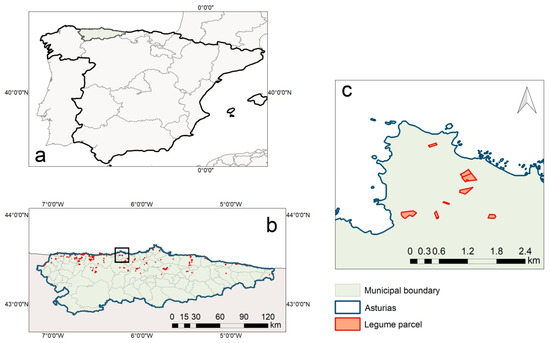
Figure 1.
(a) Location of Asturias within Spain; (b) spatial distribution of legume parcels across Asturias; (c) zoom-in view displaying legume parcels within a selected area.
Asturias is well known for its natural landscapes, which include mountainous areas like the Cantabrian Mountains and a coastline facing the Cantabrian Sea [64].
One of the most emblematic agricultural products found in Asturias is the bean from this region, a legume that has been certified as a Protected Geographical Indication (PGI).
The certification was obtained in 1990 with the ORDEN 6 DE JULIO DE 1990 (BOE of 17), under which the regulation of the specific denomination “Faba Asturiana” and its regulatory council was ratified [65].
The use of chemical herbicides is prohibited, with traditional and environmentally friendly farming practices prioritized [66]. In Figure 1, the cadastral parcels of production of this legume are shown.
The bean of the Asturias region is highly valued for its exceptional quality, characterized by its optimal size, thin skin, and buttery texture. This makes it ideal for iconic regional dishes like “fabada asturiana”, a rich stew prepared with white beans and various meats such as sausage, ham, lard, and bacon [67]. Its cultivation reflects Asturias’ agricultural traditions, emphasizing sustainable and environmentally respectful practices [68].
2.2. Methods
The methodology developed in this research was designed to be applied in several areas, even those that differ significantly. This would then allow its suitability and, consequently, its applicability across all EU territories to be verified [69]. The analysis was conducted based on cadastral parcels where the legume is cultivated within the Asturian region. The cadastral data were provided by the Bean of Asturias Region Production Consortium through a reference code that enabled us to map the entire territory using QGIS [70,71].
The significance of this methodology lies in its ability to evaluate environmental sustainability in the production area of any PGI-certified legume.
The proposed methodology consists of three general phases (Figure 2). With this methodology, we aim to conduct a thorough evaluation of environmental sustainability within the selected region, facilitating its application to other cultivation areas of quality-certified legumes based on their respective cadastral parcels.
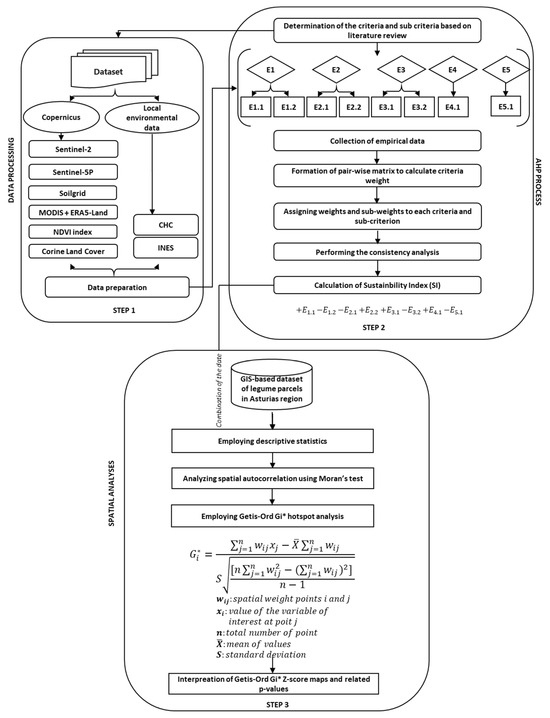
Figure 2.
Proposed methodology for evaluating environmental sustainability in a territory where a quality-certified legume is cultivated.
The methodological phases are:
Step I: Data Processing. Data processing involves collecting information from both local and satellite sources, as well as analysing it within the specific context under consideration. In some cases, satellite sources are not utilized because local data provide a more comprehensive analysis. Further details are presented in Figure 2 and Table 1. When choosing the data, we first considered local environmental data and encountered problems with the distance between the environmental survey stations and the cadastral parcels. When the survey station was too far away from the parcels, we took satellite data into account.

Table 1.
Indicators, sub-indicators, and sources from which the data were retrieved.
Step II: Analytic Hierarchy Process (AHP). The data collected from various available databases for each sub-indicator were reprocessed using the Analytic Hierarchy Process (AHP). Specifically, a Saaty matrix was constructed, and twelve experts participated in this analysis. The results (Table 2) allowed us to calculate the Sustainability Index using a formula presented in Figure 2, Step 2.
Table 2.
Weights obtained for each indicator.
Step III: Spatial Analysis. A descriptive statistical analysis was conducted through a correlation matrix (Table 3) and violin plots. The data were analyzed using a territorial analysis system, QGIS, which enabled us to map the territory and visually represent the obtained results, both for individual sub-indicators and for overall sustainability at the end of the analysis. Additionally, a spatial autocorrelation analysis was performed using Moran’s I and hotspot analysis through the Getis-Ord Gi* method. A summary of the methodology is presented here, followed by a detailed description of the three phases.
Table 3.
Detailed analysis of violin plots.
2.2.1. Step I: Data Processing
The study and analysis of the indicators and sub-indicators began with the Guidelines for the Sustainability Assessment of Food and Agriculture Systems (SAFA) [72], which form the foundation for the sustainability analysis presented in this work (Figure 3). These guidelines were developed to evaluate the impact of food and agricultural activities on the environment and society.
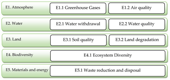
Figure 3.
Summary diagram of indicators and sub-indicators.
The aim, therefore, is to provide standardized metrics to guide future sustainability assessments, specifically in the case of Protected Geographical Indication (PGI) products. This analysis focused exclusively on the environmental dimension, as agriculture plays a crucial role in promoting sustainability in this specific context.
In this phase, we aim to analyse the main indicators that define environmental sustainability in the cultivation of quality-certified legumes. The selected indicators were defined based on sub-indicators that enable the evaluation of the sustainability of a given territory based on the collected information. The selected criteria and their descriptions are presented in Table 1.
2.2.2. Step II: Analytic Hierarchy Process (AHP)
For the calculation, twelve experts, divided into four agricultural engineers, four legume production experts, and four environmental experts were asked to evaluate the indicators by comparing them with each other using a Saaty matrix [94]. The Saaty matrix is a tool used in the Analytic Hierarchy Process (AHP), and is a multicriteria decision-making method developed by Thomas L. Saaty in the 1970s. This method facilitates complex decision making by considering multiple criteria and alternatives. In this matrix, the weight of each variable is calculated through a pairwise comparison process. Each expert compares all variables in pairs, assigning a preference value according to Saaty’s scale (1 to 7 or 1 to 1/7). The vector of normalised weights is calculated. The final weights are obtained by normalising the values of the resulting matrix. The consistency index (CI) and consistency ratio (CR) are calculated to ensure that the ratings are consistent. A CR of less than 0.1 is generally acceptable. The judgements of the 12 experts are aggregated. This can be performed by calculating the geometric mean of the values assigned by each expert for each pairwise comparison [95,96].
The averages of the values assigned by the experts are represented in Table 2. The table presents the weights obtained for each indicator.
2.2.3. Step III: Spatial Analysis
Several statistical analyses were conducted.
Pearson Correlation Matrix
The Pearson correlation matrix is a statistical tool that presents the correlations between multiple variables in a dataset [97,98,99]. It is based on the Pearson correlation coefficient (r), which measures the linear relationship between two numerical variables (Equation (1)).
in which:
Density Distribution Through a Violin Graph
A violin plot is a data visualization tool that combines the features of a box plot and a kernel density plot [100]. The distribution of data is represented by the shape of the violin plot. The wider sections indicate a higher concentration of data within that range, while the narrower sections signify fewer values. The overall shape of the violin plot visually illustrates how data values are distributed across different ranges.
Moran’s I Test
The Moran’s I test is a spatial analysis tool that provides insights into the spatial distribution of data [101]. This tool allows us to observe the spatial autocorrelation of the data, determining whether the observed values exhibit a clustered, random, or dispersed pattern. The dataset was initially loaded and preprocessed to transform the target variable, the Sustainability Index, into a numerical format and remove any missing values.
Getis-Ord Gi* Statistics
The Getis-Ord Gi* statistic is a spatial analytical technique employed to identify clusters of elevated or diminished values within a geographical distribution [102]. It assesses whether spatial characteristics display significant hotspots (high-value clustering) or cold spots (low-value clustering) by contrasting local observations with the overall spatial distribution [103].
This technique enables the identification of notable clusters in space with either higher or lower values. Specifically, the Gi* value is obtained by evaluating each point in the dataset to determine the local value concentration of values around it. The Gi* values are then compared to a random distribution to determine whether the observed clusters are statistical negative Gi* values, which indicate clusters of low values (cold spots). From this analysis, two different types of maps can be generated.
The approach relies on a weighted sum of adjacent data, with the Gi* statistic computed for each geographic unit according to Equation (2):
in which:
The resultant Z-score quantifies the statistical importance of clustering, signifying whether observed spatial patterns diverge from chance. A high positive Z-score indicates that a site and its surrounding areas possess values greater than anticipated in a random distribution, designating it as a hotspot. A low negative Z-score signifies a concentration of low values, identifying it as a cold area. The associated p-value establishes the confidence level of these clusters, with thresholds set at 90%, 95%, or 99% confidence intervals.
3. Results
3.1. Initial Data Exploration and Statistical Analysis
3.1.1. Correlation Matrix
In this study, to assess environmental sustainability, values from every indicator of the variable were placed into a Pearson correlation matrix [104], Figure 4. Afterwards, the results were interpreted accurately and holistically with the help of multivariate analysis tools.
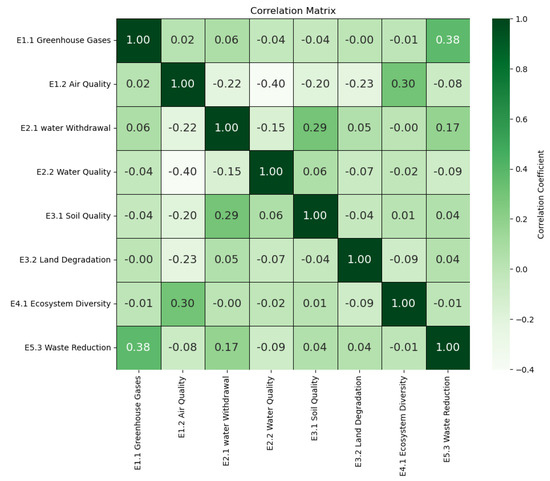
Figure 4.
Correlation matrix of various environmental indicators, with positive correlations in dark green and negative correlations in light green.
The correlation matrix results enable us to display the degree of relation between various variables in the table using colour to interpret a correlation matrix; it is important to consider the strongest correlations (both positive and negative), as they are more significant and can indicate important relationships between different environmental indicators.
Correlations above 0.8 or below −0.8 are considered high since they indicate a strong relation between two variables. Moderate correlations range from 0.3 to 0.7, while those between –0.3 and –0.7 also indicate a moderate correlation [105,106]. In this study, the correlation that exists between E2.2 Water Quality and E4.1 Ecosystem Diversity is moderate at 0.78. The established correlation between water quality and ecosystem diversity indicates that enhancing water conditions may positively influence ecosystem biodiversity. These findings can be ascribed to the direct impact of water quality on the health of natural ecosystems and the diversity of organisms residing within them. E1.1 Greenhouse Gases have a positive correlation with E2.1 Water Withdrawal (0.85), which means an increase in greenhouse gases is associated with more water withdrawal. However, it is important to clarify that correlation does not inherently imply causation. E2.2 Water Quality also has a positive correlation with E4.1 Ecosystem Diversity (0.78), meaning that better water quality brings better ecosystem diversity.
Negative correlations are those in which the increase in one variable corresponds with the decrease in the other. The relationship between E3.1 Soil Quality and E5.1 Waste Reduction exhibits a negative correlation of −0.75, meaning that improved soil quality accompanies a decrease in waste. This correlation can be explained by sustainable waste management practices and natural resource-efficient initiatives.
Another negative correlation is observed between E1.2 Air Quality and E3.2 Land Degradation (−0.68), indicating that better air quality is associated with lower land degradation. Reducing air pollution can improve soil quality by integrating undesirable factors like acidification, heavy metals, and chemicals in soils.
3.1.2. Distribution and Density of the Data
Another type of analysis conducted concerns the allocation of each indicator, showing the dispersion and concentration of information. The aim of this analysis is to show how indicator values are dispersed or concentrated. This analysis is represented graphically using the so-called violin plot, a data visualisation tool that combines the characteristics of a box plot with an estimate of kernel density.
This enables a clear and detailed visualisation of how the indicator values are distributed, highlighting both the dispersion and concentration of information (Figure 5).
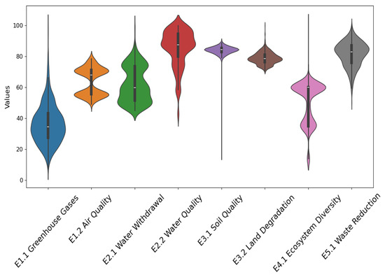
Figure 5.
Violin graph illustrating the distribution of values for each indicator, showing the variability and density of the data.
The violin plot may take on a symmetric shape, indicating that the data are evenly distributed. If it has an asymmetric shape, the data are distributed unevenly. Outliers are observable as points outside the violin. These values lie far from most of the data and can help identify anomalies or exceptional values within the dataset. Table 3 shows the statistics corresponding to the plotted violins.
As can be observed in Figure 5, the indicators E2.1 Water Withdrawal, E2.2 Water Quality, and E4.1 Ecosystem Diversity are highly asymmetric, which implies that the values corresponding to these indicators do not follow a defined pattern. In contrast, E1.2 Air Quality, E3.1 Soil Quality, E3.2 Land Degradation, and E5.1 Waste Reduction are more evenly distributed so there is less variability for these indicators. Furthermore, certain indicators have elongated tails in either direction, suggesting the potential existence of extreme values or outliers.
In Figure 6, the values corresponding to the various indicators for each of the considered land parcels are highlighted. The values are normalized to 100, so a different colour is used for each interval taken into account. The result is shown in a table in the document attached to this article.
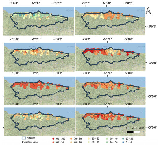
Figure 6.
Results for the various indicators. Starting from the top left, we have: E1.1, E1.2, E2.1, E2.2, E3.1, E3.2, E4.1, and E5.1.
Figure 7 displays the result of the sustainability values for each distinct parcel. The values are presented in a table in the document attached to this article (Table S1).
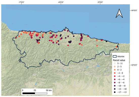
Figure 7.
Sustainability results in the various land parcels.
3.2. Moran’s I Test
The spatial weight matrix was constructed using the K-Nearest Neighbours (KNN) approach, linking each observation to its five nearest neighbours (k = 5) to define its spatial associations. The matrix was row normalized following the W-style, which guarantees equal attention to all weighted observations.
The Moran’s I test was then performed under the assumption of randomization, where the null hypothesis states that the spatial distribution of data is random. The analysis produced several key measures that are presented in Table 4.
Table 4.
Moran’s I test results.
The calculated Moran’s I statistic was 0.74555, signifying a robust positive spatial autocorrelation.
The analysis shows that the expected randomized value of Moran’s I was −0.00164. This indicates that the observed value is significantly higher than what would be expected in a context without a defined geographical structure. Additionally, the variance of Moran’s I, which is 0.0005539, suggests a low level of uncertainty in the estimation, thereby enhancing the reliability of the results.
The Z-score of 31.75 gives us confirmation that the observed pattern is not causally distributed, as the value is much higher than the threshold value of statistical significance, which is Z > 1.96. Furthermore, the p-value of less than 0.01 indicates to us the fact that the spatial aggregation observed is highly significant and therefore not random.
3.3. Getis-Ord Gi* Statistics
The Z-score map (or Z-Map), is shown in Figure 8 (top), and the p-value map is displayed in Figure 8 (bottom).
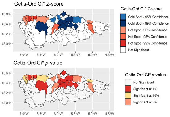
Figure 8.
Getis-Ord Gi* hotspot and cold spot analysis.
Using the Getis-Ord Gi*, the spatial distribution of the Z-score in the upper map (Figure 8) allows for the identification of hotspots (in red) and cold spots (in blue) as spatial clusters. The analysis has shown that the northern portions of Asturias, particularly the central and eastern coastal areas (Gijón, Avilés, and the Oviedo area), as well as the central-western area in the municipality of Tineo, present statistically significant cold spots with confidence levels of 95% and 99%. This means that there is a spatial concentration of low values for the analysed variable in these regions.
The hotspots with higher confidence levels (99%) are in the northwestern area, in the municipalities of El Franco and Navia. Lowering to a confidence level of 95%, three well-defined blocks appear: northwest (Tapia de Casariego and Coaña), central Asturias in Grado, and the eastern area in Cangas de Onís.
The second map (Figure 8) examines the significance of the detected clusters, applying p-values to measure the strength of the identified spatial aggregations. The dark red areas present regions of highly significant clusters at the 1% threshold, especially in the central area of the region (Gijón, Avilés, and the Oviedo area), which correspond to the cold spots observed in the Z-score map, as well as in the northwestern area (El Franco and Navia) represented as hotspots with 99% confidence. The municipality of Tineo also shows highly significant values.
The yellow regions (10% significance) and orange regions (5% significance) indicate a pronounced but still present level of clustering, occurring along the coastal regions and in the western mountain ranges. In the 5% significance areas, three blocks are observed: one in the northwest (Tapia de Casariego and Coaña), a central area (Grado, Pravia, Castrillón, and Illas), and in the eastern area in Cangas de Onís.
Regarding the areas with 10% significance, three isolated municipalities are shown, all located in the northern part of Asturias, bordering the Cantabrian Sea. As in the previous case, the large extent of blank space confirms that a significant part of the region is unclustered.
This region does not present a systematic spatial pattern, as it is not the most suitable area for bean cultivation.
In the upper image (Figure 8), the spatial arrangement of the Z-score, applying the Getis-Ord Gi* technique, facilitates the detection of hotspots (in red) and cold spots (in blue) as spatial clusters. The study reveals that the northern regions of Asturias, especially the central and eastern coastal areas (Gijón, Avilés, and the Oviedo region), together with the central-western part of the municipality of Tineo, present statistically significant cold spots with confidence levels of 95% and 99%, reflecting a spatial concentration of low values for the analysed variable. Conversely, the areas identified as hotspots with a confidence level of 99% are located in the northwestern region, specifically in the municipalities of El Franco and Navia. Meanwhile, with a confidence level of 95%, three prominent clusters stand out: the northwest (including Tapia de Casariego and Coaña), the central region of Asturias around Grado, and the eastern area in Cangas de Onís. The large empty areas in certain regions, particularly in southern Asturias, highlight zones without significant spatial patterns, generally mountainous regions characterized by cooler temperatures and less favourable conditions for faba bean cultivation.
In the lower image (Figure 8), the significance of the identified clusters is evaluated by means of p-values, which allows us to review the intensity of the spatial groupings detected. The regions in dark red, indicating clusters of high significance at the 1% threshold, are located in the central area (Gijón, Avilés, and the Oviedo region), coinciding with the cold spots shown in the Z-score map, as well as in the northwest section (El Franco and Navia), where the hotspots with 99% confidence are located. The municipality of Tineo also exhibits very significant values. The areas in yellow (10% significance) and orange (5% significance) indicate a lower but still present level of clustering, especially in the coastal areas and western mountain ranges, with three well-defined clusters in the northwest (Tapia de Casariego and Coaña), the central region (Grado, Pravia, Castrillón, and Illas), and the eastern area in Cangas de Onís. In addition, areas with 10% significance include three isolated municipalities located in the northern part of Asturias, adjacent to the Cantabrian Sea.
4. Discussion
4.1. Data Correlation and Distribution
The obtained results can be attributed to the direct impact of water quality on the health of natural ecosystems and the diversity of organisms residing in them. It is essential to recognise that this relationship is neither deterministic nor incontrovertible; instead, it is moderate, with a correlation coefficient indicating a link without implying direct causation. It is important to consider that other elements such as the handling of land, farming techniques, presence of some pollutants, and other climate changes may impact the connection between water quality and ecosystem diversity significantly [90]. Therefore, integrating other factors in a single study could improve the understanding of the relationships between these environmental variables and their dynamics.
The colours in Figure 4 run from dark green to very light green. Strong correlations can also be positive, meaning that when one variable increases, the other also increases.
In this context, while the observed relationship suggests that regions or sectors with higher water withdrawal tend to report elevated greenhouse gas emissions, this association might be influenced by additional confounding factors—such as industrial activity, energy consumption patterns, or regional climatic variations—that were not fully isolated in the analysis.
Newer research has stressed that effective waste management through recycling, composting, and reducing non-biodegradable waste can improve soil quality and reduce pollution [107]. Circular economy policies and integrated waste management lead to a better use of natural resources and, hence, lower the environmental burden while increasing the sustainability of production systems [108]. This provides support to the argument that there can be significant changes in soil quality and waste minimization through targeted efforts in these areas.
Researchers assert that the impact of aerial contaminants, including sulphur dioxide (SO2), nitrogen oxides (NOx), and fine particulate matter (PM), results in modification of the soil’s pH, nutrient availability, and microbial diversity, which is important for soil fertility [109].
Through more enforcement of environmental regulations and better control of industrial vehicles, the emission of such compounds has been lowered, resulting in decreased acid deposition. This has led to improved soil regeneration and even enhanced terrestrial ecosystems [110]. Research by the European Environment Agency (EEA2020) [111] suggests a link between lower air pollution and improved soil quality in areas that have been previously polluted by dangerous chemicals. These data validate the theory that reducing the emission of air pollutants results in an ecological restoration geochemical cycle in soil, reducing contamination issues while increasing sustainability of the environment.
Continuous ecosystem monitoring is essential to evaluate long-term impacts and guarantee appropriate soil protection efforts.
To ascertain a true cause-and-effect relationship, further analysis would be required. This could involve the application of multivariate regression models that control for potential confounders, or longitudinal studies designed to observe the temporal sequence of changes in both variables. As it stands, our correlation analysis merely reflects an association between the two variables rather than providing definitive evidence of a direct causal mechanism.
The violin plot shows the distribution of the data across quartiles, highlighting the median, while the Kernel Density estimation provides a representation of the distribution by showing the density of values along the interval. This enables a clear and detailed visualisation of how the indicator values are distributed, highlighting both the dispersion and concentration of information (Figure 5).
These values lie far from most of the data and can help identify anomalies or exceptional values within the dataset. Table 3 shows the statistics corresponding to the plotted violins.
This indicates that regions with elevated Sustainability Index values are markedly clustered, whereas regions with diminished values are similarly clustered. This result suggests that the distribution of the index is not random but follows a defined spatial pattern.
4.2. Moran’s I Test
The results of the analyses suggest that the Sustainability Index is not randomly distributed but rather follows a clear spatial pattern. Specifically, what can be observed is a tendency for similar values to cluster together rather than being dispersed. This highlights the presence of a model that shows the correct distribution of sustainability within the considered territory.
This evidence is highly significant, as it demonstrates that environmental sustainability is not uniformly distributed but is instead concentrated in specific areas with systematically high or low values. Such distribution may be influenced by numerous factors, including the natural characteristics of the territory, local environmental policies, and patterns of urbanization and land use. The low variance observed (0.0005539) further confirms the precision of Moran’s I estimation, reducing the margin of uncertainty and strengthening the robustness of the results. The fact that the observed pattern is highly unlikely to result from random sampling suggests that the detected high spatial autocorrelation is a genuine phenomenon rather than an artifact of the analysis.
The detected model is statistically significant across multiple levels of analysis. This is evidenced by the high spatial correlation and contained variance. This implies that environmental sustainability in this region is linked to specific territorial dynamics, which must be considered in environmental planning and management strategies.
Analysis of the distribution of the Sustainability Index shows that it is strongly modulated by external factors such as environmental conditions, land management, and type of land use. These factors interact in a complex way, leading to the formation of groups of areas with similar ecological quality ratings, which underlines the importance of considering ecological connections between adjacent regions to improve overall environmental sustainability. This evidence is in line with studies by Turner, Lambin, and Reenberg, who documented how land-use changes follow specific spatial patterns, influenced by environmental and socioeconomic variables [112].
The further confirmation that sustainability is not distributed homogeneously but follows well-defined spatial patterns is of fundamental importance for the development of effective environmental policies. In fact, the integration of territorial peculiarities in the sustainable management of resources is an essential element for environmental protection, as it enables the development of targeted interventions that take into account the ecological specificities of each area. This perspective is also reflected in the analyses of Lambin and Meyfroidt, as well as those of Pretty, who highlight how spatial planning based on an integrated assessment of environmental factors favours more sustainable and resilient management strategies [109]
4.3. Getis-Ord Gi* Statistics
The large blank spaces observed in some areas, especially throughout the southern region of Asturias, denote regions of less interesting geography that do not present relevant spatial patterns, meaning that the values in these regions lack a statistically significant spatial distribution. These areas tend to be more mountainous, which implies lower temperatures and more challenging conditions for growing faba beans.
These results highlight the importance of developing agricultural sustainability policies tailored to local conditions, rather than applying general and uniform approaches based on broad principles of sustainable agriculture. The autocorrelation and spatial clustering maps reveal key opportunities to implement sustainable farming methods, especially in PGI-certified areas, with the aim of improving sustainability in low-yielding regions and fostering innovative farming practices in high-yielding areas. To ensure long-term ecological and agricultural resilience, it is critical to complement these efforts with policies that consider environmental changes and provide a comprehensive strategy for continuous improvement of sustainability in relation to ecological quality over time.
5. Conclusions
The study highlights that environmental sustainability in Asturias has different spatial patterns, with some areas consistently showing high index values and other areas showing low ones. Significant correlations were identified between various environmental indicators: higher water quality is associated with greater ecosystem diversity, while increased greenhouse gas emissions correlate with higher water withdrawal. Similarly, better air and soil quality tends to coincide with less environmental degradation and reduced waste production.
Spatial analysis confirms that sustainability levels are not randomly distributed but instead form coherent geographical clusters. Urban areas in the central and eastern coastal regions show lower sustainability performance, while northwestern and rural areas demonstrate more favourable environmental conditions. This indicates that geographical, political, or social factors play a significant role in shaping these patterns, highlighting how local policies that recognize the specific characteristics of each territory play an important role.
The results underline the need to adapt appropriate environmental and agricultural policies that adapt to the specific characteristics of each region, promoting differentiated strategies that effectively address local ecological, social, and economic conditions.
Supplementary Materials
The following supporting information can be downloaded at: https://www.mdpi.com/article/10.3390/land14030636/s1, Table S1: Table with all values.
Author Contributions
B.C.: writing—original draft preparation, visualization, and investigation. J.V.: conceptualization, methodology, investigation, and supervision. D.G.: data curation, writing—reviewing and editing, and supervision. C.L.: data curation and writing—reviewing and editing. V.R.: methodology and writing—reviewing and editing. All authors have read and agreed to the published version of the manuscript.
Funding
Fundaçao para a Ciencia e a Tecnologia: UIDB/05064/2020.
Data Availability Statement
The original contributions presented in the study are included in the article; further inquiries can be directed to the corresponding author.
Conflicts of Interest
Author Víctor Rincón were employed by Tragsatec. The remaining authors declare that the research was conducted in the absence of any commercial or financial relationships that could be construed as a potential conflict of interest. Tragsatec partially financed the project. The funders had no role in the design of the study; in the collection, analyses, or interpretation of data; in the writing of the manuscript, or in the decision to publish the results.
References
- Keys, A. Mediterranean Diet and Public Health: Personal Reflections. Am. J. Clin. Nutr. 1995, 61 (Suppl. S6), 1321S–1323S. [Google Scholar] [CrossRef]
- Sofi, F.; Cesari, F.; Abbate, R.; Gensini, G.F.; Casini, A. Adherence to Mediterranean Diet and Health Status: Meta-Analysis. BMJ 2008, 337, a1344. [Google Scholar] [CrossRef] [PubMed]
- Estruch, R.; Ros, E.; Salas-Salvadó, J.; Covas, M.I.; Corella, D.; Arós, F.; Gómez-Gracia, E.; Ruiz-Gutiérrez, V.; Fiol, M.; Lapetra, J.; et al. Primary Prevention of Cardiovascular Disease with a Mediterranean Diet. N. Engl. J. Med. 2013, 368, 1279–1290. [Google Scholar] [CrossRef] [PubMed]
- Trichopoulou, A.; Costacou, T.; Bamia, C.; Trichopoulos, D. Adherence to a Mediterrane-an Diet and Survival in a Greek Population. N. Engl. J. Med. 2003, 348, 2599–2608. [Google Scholar] [CrossRef]
- UNESCO. Mediterranean Diet: Inscribed in 2010 on the Representative List of the Intangible Cultural Heritage of Humanity. Available online: https://ich.unesco.org. (accessed on 31 January 2025).
- Willett, W.C.; Sacks, F.; Trichopoulou, A.; Drescher, G.; Ferro-Luzzi, A.; Helsing, E.; Trichopoulos, D. Mediterranean Diet Pyramid: A Cultural Model for Healthy Eating. Am. J. Clin. Nutr. 1995, 61, 1402S–1406S. [Google Scholar] [CrossRef] [PubMed]
- Bach-Faig, A.; Berry, E.M.; Lairon, D.; Reguant, J.; Trichopoulou, A.; Dernini, S.; Medina, F.X.; Battino, M.; Belahsen, R.; Miranda, G.; et al. Mediterranean Diet Pyramid Today. Science and Cultural Updates. Public Health Nutr. 2011, 14, 2274–2284. [Google Scholar] [CrossRef]
- Trichopoulou, A.; Martínez-González, M.A.; Tong, T.Y.; Forouhi, N.G.; Khandelwal, S.; Prabhakaran, D.; Mozaffarian, D.; de Lorgeril, M. Definitions and Potential Health Benefits of the Mediterranean Diet: Views from Experts around the World. BMC Med. 2014, 12, 112. [Google Scholar] [CrossRef]
- Schwingshackl, L.; Missbach, B.; König, J.; Hoffmann, G. Adherence to a Mediterranean Diet and Risk of Diabetes: A Systematic Review and Meta-Analysis. Public Health Nutr. 2014, 17, 1757–1769. [Google Scholar] [CrossRef]
- Esposito, K.; Kastorini, C.M.; Panagiotakos, D.B.; Giugliano, D. Mediterranean Diet and Weight Loss: Meta-Analysis of Randomized Controlled Trials. Metab. Syndr. Relat. Disord. 2011, 9, 1–12. [Google Scholar] [CrossRef]
- Rosato, V.; Temple, N.J.; La Vecchia, C.; Castellan, G.; Tavani, A.; Guercio, V. Mediterranean Diet and Cardiovascular Disease: A Systematic Review and Meta-Analysis of Observational Studies. Eur. J. Nutr. 2019, 58, 173–191. [Google Scholar] [CrossRef]
- Schwingshackl, L.; Hoffmann, G. Adherence to Mediterranean Diet and Risk of Cancer: An Updated Systematic Review and Meta-Analysis of Observational Studies. Cancer Med. 2015, 4, 1933–1947. [Google Scholar] [CrossRef] [PubMed]
- Sofi, F.; Macchi, C.; Abbate, R.; Gensini, G.F.; Casini, A. Mediterranean Diet and Health Status: An Updated Meta-Analysis and a Proposal for a Literature-Based Adherence Score. Public Health Nutr. 2014, 17, 2769–2782. [Google Scholar] [CrossRef]
- Dernini, S.; Berry, E.M. Mediterranean Diet: From a Healthy Diet to a Sustainable Dietary Pattern. Front. Nutr. 2015, 2, 15. [Google Scholar] [CrossRef]
- Jensen, E.S.; Peoples, M.B.; Hauggaard-Nielsen, H. Faba Bean in Cropping Systems. Field Crops Res. 2010, 115, 203–216. [Google Scholar] [CrossRef]
- Peoples, M.B.; Herridge, D.F.; Ladha, J.K. Biological Nitrogen Fixation: An Efficient Source of Nitrogen for Sustainable Agricultural Production? Plant Soil 1995, 174, 3–28. [Google Scholar] [CrossRef]
- Stagnari, F.; Maggio, A.; Galieni, A.; Pisante, M. Multiple Benefits of Legumes for Agriculture Sustainability: An Overview. Chem. Biol. Technol. Agric. 2017, 4, 2. [Google Scholar] [CrossRef]
- Donini, L.M.; Serra-Majem, L.; Bulló, M.; Gil, Á.; Salas-Salvadó, J. The Mediterranean Diet: Culture, Health and Science. Br. J. Nutr. 2015, 113, S1–S3. [Google Scholar] [CrossRef]
- Altieri, M.A.; Nicholls, C.I.; Henao, A.; Lana, M.A. Agroecology and the Design of Climate-Resilient Farming Systems. Agron. Sustain. Dev. 2015, 35, 869–890. [Google Scholar] [CrossRef]
- Gliessman, S.R. Transforming Food Systems with Agroecology. Agron. Sustain. Dev. 2016, 40, 187–189. [Google Scholar] [CrossRef]
- Wezel, A.; Bellon, S.; Doré, T.; Francis, C.; Vallod, D.; David, C. Agroecology as a Science, a Movement and a Practice. A Review. Agron. Sustain. Dev. 2009, 29, 503–515. [Google Scholar] [CrossRef]
- Food and Agriculture Organization of the United Nations. Sustainable Development and Natural Resources Management. In Proceedings of the FAO Conference 25th Session, Rome, Italy, 11–29 November 1989. [Google Scholar]
- Grosso, G.; Fresán, U.; Bes-Rastrollo, M.; Marventano, S.; Galvano, F. Environmental Impact of Dietary Choices: Role of the Mediterranean and Other Dietary Patterns in an Italian Cohort. Int. J. Environ. Res. Public Health 2020, 17, 1468. [Google Scholar] [CrossRef] [PubMed]
- Galli, F.; Favilli, E.; D’Amico, S.; Brunori, G. The Mediterranean Diet as a Lever for Sustainable Development: The Four Dimensions of Sustainability. Sustainability 2020, 12, 6147. [Google Scholar]
- González Fischer, C.; Garnett, T. Plates, Pyramids, Planet: Developments in National Healthy and Sustainable Dietary Guidelines: A State of Play Assessment; FAO: Rome, Italy; The University of Oxford: Oxford, UK, 2016. [Google Scholar]
- United Nations. Transforming Our World: The 2030 Agenda for Sustainable Development; UN General Assembly, A/RES/70/1; UN: New York, NY, USA, 2015. [Google Scholar]
- Sachs, J.D. The Age of Sustainable Development; Columbia University Press: New York, NY, USA, 2015. [Google Scholar]
- Griggs, D.; Stafford-Smith, M.; Gaffney, O.; Rockström, J.; Öhman, M.C.; Shyamsundar, P.; Noble, I. Sustainable Development Goals for People and Planet. Nature 2013, 495, 305–307. [Google Scholar] [CrossRef] [PubMed]
- United Nations Department of Economic and Social Affairs. The Sustainable Development Goals Report 2020; United Nations: New York, NY, USA, 2020; ISBN 978-92-1-101425-9. Available online: https://www.un.org/en/desa/sustainable-development-goals-report-2020 (accessed on 11 March 2025).
- Johnston, J.L.; Fanzo, J.C.; Cogill, B. Understanding Sustainable Diets: A Descriptive Analysis of the Determinants and Processes that Influence Diets and Their Impact on Health, Society and the Environment. Adv. Nutr. 2014, 5, 418–429. [Google Scholar] [CrossRef] [PubMed]
- Fanzo, J.; Davis, C.; McLaren, R.; Choufani, J. The Effect of Sustainable Diets on Food Security and Nutrition. Glob. Food Secur. 2020, 24, 100356. [Google Scholar]
- Gollin, D. Conserving Genetic Resources for Agriculture: Economic Implications of Emerging Science. Food Secur. 2020, 12, 919–927. [Google Scholar] [CrossRef]
- Food and Agriculture Organization of the United Nations. Proportion of Agricultural Area Under Productive and Sustainable Agriculture (SDG Indicator 2.4.1); FAO: Rome, Italy, 2023. [Google Scholar]
- FAO. Sustainable Agriculture for Biodiversity: Managing Agricultural Biodiversity for Sustainable Development; FAO: Rome, Italy, 2020. [Google Scholar]
- Gobierno del Principado de Asturias. Presupuestos Generales del Principado de Asturias 2022. Portal de Transparencia del Principado de Asturias. Available online: https://transparencia.asturias.es/web/gobierno-abierto/detalle?articleId=2653114&p_r_p_categoryId=694576 (accessed on 4 March 2025).
- Sharma, P.; Sharma, P.; Thakur, N. Sustainable Farming Practices and Soil Health: A Pathway to Achieving SDGs and Future Prospects. Discov. Sustain. 2024, 5, 250. [Google Scholar] [CrossRef]
- Lal, R. Soil Health and Climate Change: An Overview. J. Soil Water Conserv. 2020, 75, 123A–129A. [Google Scholar] [CrossRef]
- Gliessman, S.R. Agroecology: The Ecology of Sustainable Food Systems; CRC Press: Boca Raton, FL, USA, 2014. [Google Scholar]
- Altieri, M.A. Agroecology: The Science of Sustainable Agriculture; Westview Press: Boulder, CO, USA, 1999. [Google Scholar]
- Food and Agriculture Organization (FAO). The State of Food and Agriculture 2020; FAO: Rome, Italy, 2020. [Google Scholar]
- European Union. Regulation (EU) No 1151/2012 of the European Parliament and of the Council on Quality Schemes for Agricultural Products and Foodstuffs. Off. J. Eur. Union 2012, 343, 1–29. [Google Scholar]
- Belletti, G.; Marescotti, A.; Touzard, J.M. Geographical Indications, Public Goods, and Sustainable Development: The Roles of Actors’ Strategies and Public Policies. World Dev. 2015, 98, 45–57. [Google Scholar] [CrossRef]
- Hajjar, R.; Jarvis, D.I.; Gemmill-Herren, B. The Utility of Crop Genetic Diversity in Maintaining Ecosystem Services. Agric. Ecosyst. Environ. 2008, 123, 261–270. [Google Scholar] [CrossRef]
- Food and Agriculture Organization of the United Nations (FAO). State of Food and Agriculture: Leveraging Sustainable Agriculture for Global Food Security; FAO Publications: Rome, Italy, 2022. [Google Scholar]
- Boros, A.; Szólik, E.; Desalegn, G.; Tőzsér, D. A Systematic Review of Opportunities and Limitations of Innovative Sustainable Agricultural Practices. Agronomy 2025, 15, 76. [Google Scholar] [CrossRef]
- He, S.; Li, L.; Lv, M.; Wang, R.; Wang, L.; Yu, S.; Gao, Z.; Li, X. PGPR: Key to Enhancing Crop Productivity and Achieving Sustainable Agriculture. Curr. Microbiol. 2024, 81, 377. [Google Scholar] [CrossRef] [PubMed]
- García, C.; Hernández, T.; Costa, F.; Ceccanti, B.; Masciandaro, G.; Nannipieri, P. Soil Enzyme Activities in a Long-Term Experiment with Organic and Inorganic Fertili-zers. Soil Biol. Biochem. 1994, 26, 1647–1654. [Google Scholar]
- Sánchez, J.; Martínez, J.; González, M. Environmental Impact of Agricultural Practices in Spain. J. Environ. Manag. 2003, 68, 417–428. [Google Scholar]
- Moreno, J.M.; Oechel, W.C. The Role of Fire in Mediterranean-Type Ecosystems; Springer: New York, NY, USA, 1994. [Google Scholar]
- Gómez, J.A.; Giráldez, J.V.; Pastor, M.; Fereres, E. Effects of Tillage Method on Soil Physical Properties, Infiltration and Yield in an Olive Orchard. Soil Tillage Res. 1999, 52, 167–175. [Google Scholar] [CrossRef]
- Kebede, E. Contribution, Utilization, and Improvement of Legumes-Driven Biological Nitrogen Fixation in Agricultural Systems. Front. Sustain. Food Syst. 2021, 5, 767998. [Google Scholar] [CrossRef]
- Li, C.; Ban, Q.; Gao, J.; Ge, L.; Xu, R. The Role of Geographical Indication Products in Promoting Agricultural Development—A Meta-Analysis Based on Global Data. Agriculture 2024, 14, 1831. [Google Scholar] [CrossRef]
- Ranjan, V.R. Agroecological Approaches to Sustainable Development. Front. Sustain. Food Syst. 2024, 8, 1405409. [Google Scholar] [CrossRef]
- Rodríguez Madrera, R.; Campa Negrillo, A.; Ferreira Fernández, J.J. Modulation of the Nutritional and Functional Values of Common Bean by Farming System: Organic vs. Conventional. Front. Sustain. Food Syst. 2024, 7, 1282427. [Google Scholar] [CrossRef]
- Silva Martins, L.O.; de Oliveira, V.R.V.; Lora, F.A.; Fraga, I.D.; Braga Saldanha, C.; Silva, D.T.; Pereira, M.G.A.; Silva, M.S. Geographic Indications, Sustainability and Sustainable Development: A Bibliometric Analysis. J. Scientometr. Res. 2024, 13, 919–934. [Google Scholar] [CrossRef]
- Pérez, R.; Fernández, C.; Laca, A.; Laca, A. Evaluation of Environmental Impacts in Legume Crops: A Case Study of PGI White Bean Production in Southern Europe. Sustainability 2024, 16, 8024. [Google Scholar] [CrossRef]
- Abubakar, I.R.; Maniruzzaman, K.M.; Dano, U.L.; AlShihri, F.S.; AlShammari, M.S.; Ahmed, S.M.S.; Al-Gehlani, W.A.G.; Alrawaf, T.I. Environmental Sustainability Impacts of Solid Waste Management Practices in the Global South. Int. J. Environ. Res. Public Health 2022, 19, 12717. [Google Scholar] [CrossRef] [PubMed]
- Flinzberger, L.; Cebrián-Piqueras, M.A.; Peppler-Lisbach, C.; Zinngrebe, Y. Why Geographical Indications Can Support Sustainable Development in European Agri-Food Landscapes. Front. Conserv. Sci. 2022, 2, 752377. [Google Scholar] [CrossRef]
- Unger, N.; Davis, J.; Loubiere, M.; Östergren, K. Methodology for Evaluating Environmental Sustainability. EU-Refresh 2016, 5, 1–30. Available online: https://eu-refresh.org/methodology-evaluating-environmental-sustainability.html (accessed on 19 February 2025).
- Agostini, S. Effect of PDO on Rural Heritage: Integrating Origin Labelling to Promote Sustainable Rural Development in Europe. Food Nutr. J. 2016, FDNJ-103. Available online: https://www.gavinpublishers.com/article/view/effect-of-PDO-on-rural-heritage-integrating-origin-labelling-to-promote-sustainable-rural-development-in-europe (accessed on 19 February 2025).
- Augspurger, T.; Malliaraki, E.; Hopkins, J. Open Source in Environmental Sustainability. Open Sustain. Technol. Rep. 2023, 1, 1–50. [Google Scholar]
- García, N.; Fernández, J.A.; Menéndez, R.; González, J.A. Geomorphological Features and Evolution of the Asturias Region, Spain. Geomorphology 2015, 250, 1–15. [Google Scholar] [CrossRef]
- Álvarez, M.A.; Ordóñez, C.; González, J.A.; Menéndez, R. Biodiversity and Conservation of the Cantabrian Mountains in the Asturias Region. Biodivers. Conserv. 2013, 22, 1107–1125. [Google Scholar]
- López-Moreno, J.I.; Vicente-Serrano, S.M.; Moran-Tejeda, E.; Lorenzo-Lacruz, J.; Kenawy, A.; Beniston, M. Effects of Climate Change on the Intensification of the Water Cycle in the Mediterranean Region: Observations and Projections. Hydrol. Sci. J. 2011, 56, 622–640. [Google Scholar]
- Consiglio Regulador de la IGP Faba Asturiana. Normativa Faba delle Asturie. Available online: https://faba-asturiana.org/el-consejo-regulador/normativa/ (accessed on 19 February 2025).
- Faba Asturiana IGP. Qualigeo. Available online: https://www.qualigeo.eu/prodotto-qualigeo/faba-asturiana-igp/ (accessed on 15 February 2025).
- Asturian Fresh Faba. Fondazione Slow Food. Available online: https://www.fondazioneslowfood.com/en/ark-of-taste-slow-food/fresh-bean-or-green-bean/ (accessed on 15 February 2025).
- Faba Asturiana. Home-C. Available online: https://faba-asturiana.org/ (accessed on 15 February 2025).
- Zhou, P.; Ang, B.W.; Poh, K.L. Decision Analysis in Energy and Environmental Modeling: An AHP Approach. Energy 2006, 31, 2603–2616. [Google Scholar] [CrossRef]
- Malczewski, J. GIS-based Multicriteria Decision Analysis for Land Use Planning. Environ. Plan. B Plan. Des. 2004, 31, 403–428. [Google Scholar]
- Chen, Y.; Yu, J.; Khan, S. The Spatial Framework for Weighting Climate Change Impacts in a GIS Environment. Environ. Model. Softw. 2010, 25, 2041–2050. [Google Scholar]
- Food and Agriculture Organization of the United Nations. Sustainability Assessment of Food and Agriculture Systems (SAFA) Guidelines; FAO: Rome, Italy, 2012; Available online: https://www.fao.org/fileadmin/templates/nr/sustainability_pathways/docs/SAFA_Guidelines_12_June_2012_final_v2.pdf (accessed on 19 February 2025).
- Drusch, M.; Del Bello, U.; Carlier, S.; Colin, O.; Fernandez, V.; Gascon, F.; Hoersch, B.; Isola, C.; Laberinti, P.; Martimort, P.; et al. GMES Sentinel-2 Mission. Remote Sens. Environ. 2012, 120, 25–36. [Google Scholar] [CrossRef]
- Malenovský, Z.; Rott, H.; Cihlar, J.; Schaepman, M.E.; García-Santos, G.; Fernandes, R.; Berger, M. Sentinels for Science: Potential of Sentinel-1, -2, and -3 Missions for Scientific Observations of Ocean, Cryosphere, and Land. Remote Sens. Environ. 2012, 120, 84–101. [Google Scholar] [CrossRef]
- Brockmann, C. Sentinel-2 Next Generation Phase-0 Scientific Study Report; ESA: Paris, France, 2024. [Google Scholar]
- Oxoli, D.; Cedeno Jimenez, J.R.; Brovelli, M.A. Assessment of Sentinel-5P Performance for Ground-Level Air Quality Monitoring: Preparatory Experiments over the COVID-19 Lockdown Period. Int. Arch. Photogramm. Remote Sens. Spat. Inf. Sci. 2020, XLIII-B3, 123–130. [Google Scholar] [CrossRef]
- Destino, A. Valutazione Della Qualità Dell’aria Tramite Dati Satellitari; Politecnico di Torino: Turin, Italy, 2020. [Google Scholar]
- Ali, H.O.; Abraham, R.; Galerne, B. Depth Separable Architecture for Sentinel-5P Super-Resolution. arXiv 2025, arXiv:2501.17210. [Google Scholar] [CrossRef]
- Muñoz-Sabater, J.; Dutra, E.; Agustí-Panareda, A.; Albergel, C.; Arduini, G.; Balsamo, G.; Boussetta, S.; Choulga, M.; Harrigan, S.; Hersbach, H.; et al. ERA5-Land: A state-of-the-art global reanalysis dataset for land applications. Earth Syst. Sci. Data 2021, 13, 4349–4383. [Google Scholar] [CrossRef]
- Running, S.W.; Mu, Q.; Zhao, M.; Moreno, A. User’s Guide MODIS Global Terrestrial Evapotranspiration (ET) Product (NASA MOD16A2/A3); NASA Earth Observing System: Washington, DC, USA, 2017.
- Confederación Hidrográfica del Cantábrico. Inicio. Available online: https://www.chcantabrico.es/ (accessed on 15 February 2025).
- Zuazagoitia Rey-Baltar, A. Análisis del Proceso de Revisión e Implementación del Tercer Ciclo del Plan Hidrológico del Cantábrico Oriental; TFM Universidad de Alcalá: Alcalá de Henares, Spain, 2022. [Google Scholar]
- Poggio, L.; de Sousa, L.M.; Batjes, N.H.; Heuvelink, G.B.M.; Kempen, B.; Ribeiro, E.; Rossiter, D. SoilGrids 2.0: Producing soil information for the globe with quantified spatial uncertainty. SOIL 2021, 7, 217–240. [Google Scholar] [CrossRef]
- Turek, M.E.; Poggio, L.; Batjes, N.H.; Armindo, R.A.; de Jong van Lier, Q.; de Sousa, L.M.; Heuvelink, G.B.M. Global mapping of volumetric water retention at 100, 330 and 15 000 cm suction using the WoSIS database. Int. Soil Water Conserv. Res. 2023, 11, 225–239. [Google Scholar] [CrossRef]
- Hengl, T.; de Jesus, J.M.; MacMillan, R.A.; Batjes, N.H.; Heuvelink, G.B.M.; Ribeiro, E.; Samuel-Rosa, A.; Kempen, B.; Leenaars, J.G.B.; Walsh, M.G.; et al. SoilGrids1km—Global Soil Information Based on Automated Mapping. PLoS ONE 2014, 9, e105992. [Google Scholar] [CrossRef]
- García-Ruiz, J.M.; López-Moreno, J.I.; Vicente-Serrano, S.M.; Lasanta-Martínez, T.; Beguería, S. Mediterranean water resources in a global change scenario. Earth Sci. Rev. 2011, 105, 121–139. [Google Scholar] [CrossRef]
- García-Ruiz, J.M.; Nadal-Romero, E.; Lana-Renault, N.; Beguería, S. Erosion in Mediterranean Landscapes: Current Problems and Future Challenges. Land Degrad. Dev. 2013, 24, 3–15. [Google Scholar] [CrossRef]
- García-Ruiz, J.M.; Beguería, S.; Nadal-Romero, E.; Lana-Renault, N.; Sanjuán, Y.A. A meta-analysis of soil erosion rates across the world. Geomorphology 2015, 239, 160–173. [Google Scholar] [CrossRef]
- Ortiz-Burgos, S. Shannon-Weaver Diversity Index. Encycl. Earth Sci. Ser. 2015, 1, 572–573. [Google Scholar] [CrossRef]
- Ontoy, D.S.; Padua, R.N. Measuring species diversity for conservation biology: Incorporating social and ecological importance. Biodivers. J. 2014, 5, 387–390. Available online: https://www.biodiversityjournal.com/pdf/5(3)_387-390.pdf (accessed on 15 March 2025).
- Clarke, K.R.; Warwick, R.M. Changes in Marine Communities: An Approach to Statistical Analysis and Interpretation, 2nd ed.; PRIMER-E: Plymouth, UK, 2001. [Google Scholar]
- Pettorelli, N.; Vik, J.O.; Mysterud, A.; Gaillard, J.M.; Tucker, C.J.; Stenseth, N.C. Using the satellite-derived NDVI to assess ecological responses to environmental change. Trends Ecol. Evol. 2005, 20, 503–510. [Google Scholar] [CrossRef] [PubMed]
- Cavalli, S.; Penzotti, G.; Amoretti, M.; Caselli, S. A Machine Learning Approach for NDVI Forecasting based on Sentinel-2 Data. Environ. Sci. Technol. 2024, 58, 7890–7902. [Google Scholar] [CrossRef]
- Afshari, S.; Sarli, R.; Abbasnezhad Alchin, A.; Ghaffari Aliabad, O.; Moradi, F.; Saei, M.; Bakhshi Lomer, A.R.; Nasiri, V. Trend analysis and interactions between surface temperature and vegetation condition: Divergent responses across vegetation types. Environ. Monit. Assess. 2025, 197, 292. [Google Scholar] [CrossRef]
- Saaty, T.L. Decision Making with the Analytic Hierarchy Process. Int. J. Serv. Sci. 2008, 1, 83–98. [Google Scholar] [CrossRef]
- Vaidya, O.S.; Kumar, S. Analytic Hierarchy Process: An Overview of Applications. Eur. J. Oper. Res. 2006, 169, 1–29. [Google Scholar] [CrossRef]
- Pearson, K. On the Criterion That a Given System of Deviations from the Probable in the Case of a Correlated System of Variables is Such That It Can Be Reasonably Supposed to Have Arisen from Random Sampling. Lond. Edinb. Dublin Philos. Mag. J. Sci. 1900, 50, 157–175. [Google Scholar] [CrossRef]
- Ishizaka, A.; Labib, A. Review of the Main Developments in the Analytic Hierarchy Process. Expert Syst. Appl. 2011, 38, 14336–14345. [Google Scholar] [CrossRef]
- Cohen, I.; Huang, Y.; Chen, J.; Benesty, J.; Benesty, J.; Chen, J.; Cohen, I. Pearson correlation coefficient. In Noise Reduction in Speech Processing; Springer: Berlin/Heidelberg, Germany, 2009; pp. 1–4. [Google Scholar]
- Hintze, J.W.; Nelson, R.D. Violin plots: A box plot-density trace synergism. Am. Stat. 1998, 52, 181–184. [Google Scholar] [CrossRef]
- Moran, P.A.P. Notes on continuous stochastic phenomena. Biometrika 1950, 37, 17–23. [Google Scholar] [CrossRef]
- Getis, A.; Ord, J.K. The analysis of spatial association by use of distance statistics. Geogr. Anal. 1992, 24, 189–206. [Google Scholar] [CrossRef]
- Songchitruksa, P.; Zeng, X. Getis–Ord spatial statistics to identify hot spots by using incident management data. Transp. Res. Rec. 2010, 2165, 42–51. [Google Scholar] [CrossRef]
- Bobbitt, Z. What is Considered to Be a “Strong” Correlation? Statology 2020. Available online: https://www.statology.org/what-is-a-strong-correlation/ (accessed on 11 March 2025).
- Frost, J. Interpreting Correlation Coefficients; Statistics by Jim. 2020. Available online: https://statisticsbyjim.com (accessed on 11 March 2025).
- Moulton, R.L.; Taylor, R.G. Ecological Consequences of Water Quality Changes; Springer: Berlin/Heidelberg, Germany, 2012. [Google Scholar]
- Smith, R.I.; Fowler, D.; Sutton, M.A.; Flechard, C.R.; Coyle, M. Impact of Atmospheric Pollution on Soil and Water Quality in Europe. Environ. Pollut. 2015, 200, 85–93. [Google Scholar]
- Fowler, D.; Pyle, J.A.; Ravishankara, A.R.; Amann, M.; Cox, R.A.; Sanderson, M.G. The Global Impact of Air Pollution on Soil and Water Systems. Philos. Trans. R. Soc. A Math. Phys. Eng. Sci. 2009, 367, 617–640. [Google Scholar]
- Lambin, E.F.; Meyfroidt, P. Global Land Use Change, Economic Globalization, and the Looming Land Scarcity. Proc. Natl. Acad. Sci. USA 2011, 108, 3465–3472. [Google Scholar] [CrossRef]
- Turner, B.L.; Lambin, E.F.; Reenberg, A. The Emergence of Land Change Science for Global Environmental Change and Sustainability. Proc. Natl. Acad. Sci. USA 2007, 104, 20666–20671. [Google Scholar] [CrossRef] [PubMed]
- European Environment Agency (EEA). EEA Signals 2020: Towards Zero Pollution in Europe; Publications Office of the European Union: Luxembourg, 2020; Report No.: TH-AP-20-669-EN-N; ISBN 978-92-9480-267-5. ISSN 2443-7492. [CrossRef]
- Pretty, J. Agricultural Sustainability: Concepts, Principles and Evidence. Philos. Trans. R. Soc. Lond. B Biol. Sci. 2008, 363, 447–465. [Google Scholar] [CrossRef] [PubMed]
Disclaimer/Publisher’s Note: The statements, opinions and data contained in all publications are solely those of the individual author(s) and contributor(s) and not of MDPI and/or the editor(s). MDPI and/or the editor(s) disclaim responsibility for any injury to people or property resulting from any ideas, methods, instructions or products referred to in the content. |
© 2025 by the authors. Licensee MDPI, Basel, Switzerland. This article is an open access article distributed under the terms and conditions of the Creative Commons Attribution (CC BY) license (https://creativecommons.org/licenses/by/4.0/).