Global Climate Convergence from 1980 to 2022 Led to Significant Increase in Vegetation Productivity

Abstract

Changes in global temperature and precipitation over the past few decades have caused significant alterations in global climate patterns. However, the impact of these changes on global vegetation productivity remains unclear. This article evaluates the effect of converging climate patterns on global vegetation productivity, focusing on the land outside Antarctica as the study area, and theoretically substantiates the validity of the findings. The study reveals the climate status of the historical period of 1980–2022 and the SSP126 scenario, where convergence in precipitation patterns leads to a significant increase in global NPP, while the convergence of temperature patterns has a much smaller impact on NPP than precipitation. Under the high-emission scenarios SSP245 and SSP585, the laws are reversed: converging temperature patterns lead to a decrease in NPP, while converging precipitation patterns have an insignificant impact on NPP. Climate change under these three scenarios indicates the detrimental effects of climate patterns under high emissions on vegetation productivity. This study fills a gap in the literature on the impact of climate patterns on vegetation productivity.

1. Introduction

Global climate change exhibits significant spatial heterogeneity, characterized by distinct variations in key climatic parameters across different geographical regions [1,2,3]. For instance, the Arctic region is warming at a rate three times faster than the global average [4], while precipitation patterns show contrasting trends—a 20% decrease in subtropical arid zones and a 15% increase in high-latitude humid regions [5,6]. This spatial heterogeneity, driven by the synergistic effects of temperature and precipitation, and the spatial reconstruction of extreme events [7] have systematically shifted the energy distribution and water cycle paths of Earth’s surface systems [8], ultimately leading to reorganization of the global climate pattern, such as “polar acceleration of warming and humidification—subtropical persistent dry and hot conditions” [9]. Climate pattern changes have altered the living environment of vegetation, affecting the environmental suitability of plants [10,11,12,13], and reshaped the interactions within ecosystems, such as species competition and migration [14,15], which has had a profound impact on the distribution, growth, productivity, and community structure of vegetation.

Considering the backdrop of significant spatial heterogeneity in climate change, if a specific geographic unit (such as a grid) demonstrates relative stability in local climatic factors, while the climatic parameters in surrounding areas experience substantial alterations (for example, extreme warming or in the reconstruction of precipitation patterns) [7], it can become a “refuge” or an emerging suitable habitat for vegetation migration [16,17,18]. This phenomenon has been documented in the real world. For instance, mountain refuges in the Pacific Northwest maintained relatively stable climatic conditions during the last glacial period, while surrounding areas experienced significant climatic changes, making these regions long-term refuges for many species [19]. Regarding the spatial boundaries of refuges, the topographic wetness index (TWI) and temperature gradient models are generally used to quantify the spatial extent of refuges [20], or species distribution data can be combined with climate models to delineate this extent [21]. The stability of refuges mainly depends on the terrain–climate interaction mechanism. For example, complex terrain (such as mountains and canyons) can buffer the impacts of climate change by altering airflow, precipitation, and temperature distribution [22]. Not only has this vegetation response mechanism, driven by inter-regional climatic differences, caused the physical migration of species distribution ranges [23], but it also determines the type of vegetation [24]. But also, through adjustments in inter-specific competition dynamics (such as niche replacement) [25], changes can be induced in resource allocation efficiency (such as shifts in light/water use strategies), and cascading effects can be induced at the ecosystem function level (such as the restructuring of carbon and nitrogen cycles) [26], systematically reshaping the pattern of vegetation productivity. This study defines the indirect regulation of vegetation by the spatial heterogeneity of climate change as “the impact of climate patterns on vegetation productivity”. In temperate regions of the Northern Hemisphere, the average migration rate of trees is 0.1 to 1 km per year [23], whereas in alpine areas, the migration rate of herbaceous plants may be faster, reaching several kilometers per year [27]. Grassland ecosystems are capable of adapting more rapidly to climate change and can even recover productivity in the short term [15]. Although climate is the main driver of vegetation productivity, climatic factors are not the only influence, as changes in land use (such as deforestation or agricultural expansion) may obscure productivity changes driven by climate [28,29].

Due to the absence of significant changes in background climate factors, such as annual average temperature and precipitation, in the target area, traditional vegetation productivity models, including parameter models or process models based on the direct response relationships of climate parameters, struggle to effectively identify and quantify spatial correlation effects [30,31]. This issue arises because current model frameworks predominantly depend on the linear or nonlinear mapping relationship between local climate variables and vegetation productivity [31], often overlooking the ecological niche reorganization mechanism induced by regional climate gradient changes [25,32]. This cognitive gap results in systematic biases in the estimation of vegetation productivity, which, in turn, impacts the formulation of carbon policies in the context of climate change.

There are numerous examples illustrating how climate patterns affect vegetation. For instance, in the Sahel region of Africa, shifts in precipitation patterns due to climate change have had a dual impact on vegetation productivity. From the 1970s through the 1980s, the region suffered from severe droughts, resulting in a substantial decrease in vegetation cover [33]. However, in recent years, the partial recovery of precipitation has promoted the regrowth of vegetation, and there is a trend towards greening in some local areas [34]. Conversely, reduced precipitation in the surrounding regions of the southern Amazon has resulted in the proliferation of drought stress. Although precipitation in the core area remains stable, the risk of hydraulic failure, such as xylem embolism, is transferred to the core area via the decline of edge populations. This causes a nonlinear collapse of the forest carbon sink function [35].

Thus, the impact of climate patterns on vegetation is comprehensive, systematic, and indirect [36,37], rendering it challenging to estimate based on mechanisms alone. The scientific hypothesis of this study posits the following: In a region comprising multiple grids at various spatial scales, the temperature and precipitation of these grids vary while the regional averages of temperature and precipitation remain constant—indicating a change in the climate pattern. Under this ideal scenario, we can define vegetation productivity as being influenced solely by temperature and precipitation, characterizing it as a function of these two variables. Then, the alterations in regional vegetation productivity are solely due to changes in the climate pattern. The influence of climate patterns on vegetation productivity exhibits multi-scale coupling characteristics (local climate heterogeneity drives ecological processes) [37] and nonlinear transmission characteristics (energy–water redistribution triggers cascading effects) [38]. The underlying mechanism involves interactions across multiple atmosphere–biosphere–soil interfaces [39], which are difficult to effectively disentangle using traditional mechanistic models [40]. Building upon this, this study introduces a core scientific hypothesis: Assuming the regional climate averages (temperature, precipitation) remain constant, spatial heterogeneity changes in climate elements (i.e., the evolution of climate patterns) can independently induce changes in vegetation productivity. Specifically, when the temperature and precipitation of each grid within a certain area change, even though the overall climate average remains constant, the spatiotemporal differentiation of vegetation productivity can be attributed to the reconfiguration of climate patterns.

The specific scientific questions addressed by this study are as follows: How does the alteration of spatial climate patterns impact vegetation productivity in a region where the average temperature and total precipitation stay constant, and what is the mathematical correlation between climate patterns and net primary productivity? To address the aforementioned questions, this study selected temperature and precipitation anomalies as the X-axis and Y-axis, respectively. The Euclidean distance of each grid represents the difference in that grid from the global climate mean (anomaly), which we refer to as temperature convergence and precipitation convergence. Furthermore, the Euclidean distance between the grid pixel and the origin represents the climate convergence [41]. The traditional variability index is insufficient for capturing the spatial heterogeneity of extreme events [42,43]. In contrast, the convergence index utilized in this paper not only reveals the degree of deviation between regional climate and the global average, but also aids in identifying climate refuges and ecologically sensitive areas [41,44]. This study utilizes these three indicators to characterize climate patterns and ultimately fit the mathematical relationship between climate patterns and productivity. This study falls under the category of theoretical exploration, and as such, the classic climatological model, the Thornthwaite model, was selected. This model calculates potential evapotranspiration based solely on temperature and precipitation data [45], avoiding interference from vegetation dynamics, which allows for a clearer analysis of the independent effects of climatic factors. Compared to more complex ecosystem models [46], the Thornthwaite model requires only temperature and precipitation data, making it highly suitable for the data conditions of this study. In summary, it perfectly meets the technical requirements of this research, in which we compare it with another classical climatological model, the Miami model, and validate the results using the CASA model, a widely used Light Utilization Efficiency (LUE) model.

2. Materials and Methods

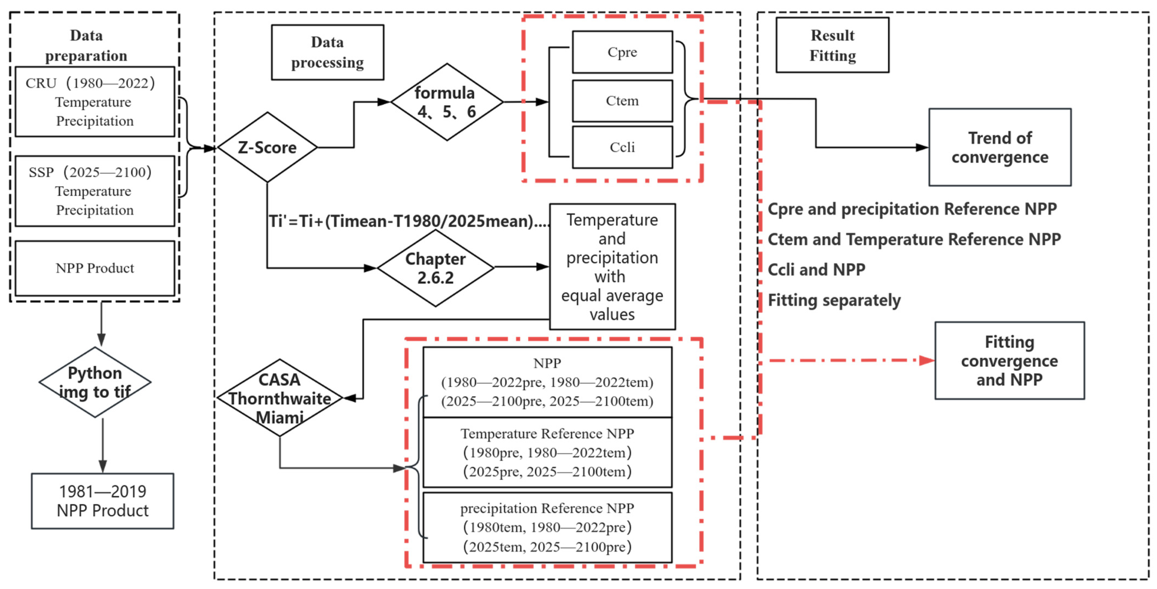
2.1. Research Flowchart

This paper maintains a constant average temperature and precipitation, employing models to estimate vegetation productivity. It then fits the mathematical relationship between climate patterns and productivity, thereby exploring the theoretical impact of climate patterns on vegetation productivity. Figure 1 illustrates the overall methodological framework of this study, encompassing three main steps: data preparation, data processing, and result fitting. The subsequent sections detail the specific methods for each step: (1) Data preparation involves the collection and preprocessing of CRU TS v4.07 temperature and precipitation data, future climate scenario data, and NPP product data. (2) Data processing includes the Z-score normalization method, baseline year adjustment, and the calculation of climate convergence; models are used to calculate NPP, including NPP estimation based on the Thornthwaite, CASA, and Miami models. (3) Result fitting entails a fitting analysis of temperature convergence with temperature baseline NPP, precipitation convergence with precipitation baseline NPP, and climate convergence with NPP.

2.2. Meteorological Data

The global temperature and precipitation data on a monthly scale were sourced from the CRU TS v4.07 data set. This data set is based on meteorological station observation data and employs interpolation methods to fill spatial gaps while also undergoing strict quality control. Consequently, it offers high accuracy in describing regional climate characteristics and has been widely applied and evaluated [47,48]. For the period 2025–2100, the SSP126, SSP245, and SSP585 scenarios were selected as the Shared Socioeconomic Pathways (SSPs) [49]. Precipitation and temperature data under these three SSPs were obtained from the NorESM2-LM and ACCESS-CM2 models [50,51], which exhibit minimal errorw and the best agreement with historical data. The data were preprocessed in ArcMap 10.8.

2.3. Vegetation Productivity Data

The historical net primary productivity (NPP) data used in this study were derived from the global daily NPP data set for the period 1981 to 2019. These data have a spatial resolution of 0.072727° × 0.072727° [52,53].

2.4. Vegetation Productivity Estimation Model

NPP is estimated using the Thornthwaite Memorial model [54], which is driven by precipitation and temperature data, as follows:

$$NPP=3000\left[1-{\mathrm{e}}^{-0.0009695(v-20)}\right]$$

(1)

$$\mathrm{V}={\displaystyle \frac{1.05\mathrm{r}}{\sqrt{1+{(1+1.05\mathrm{r}/\mathrm{L})}^2}}}$$

(2)

$$\mathrm{L}=3000+25\mathrm{t}+0.05{\mathrm{t}}^3$$

(3)

where NPP represents annual NPP (g C m⁻² yr⁻¹); V stands for the actual annual evapotranspiration (mm); L is the annual average evapotranspiration (mm); t denotes the annual average temperature (°C); and r signifies the annual precipitation (mm).

The Miami model is a classical climatological model [54] used for comparison with the results obtained from the Thornthwaite model. On the other hand, the CASA model, a LUE model with broad applicability, is employed to verify results derived from the Thornthwaite model. Its underlying mechanism fundamentally differs from that of climatological models. Our predecessors [55] believed that vegetation achieves the maximum light energy conversion rate under ideal conditions, while, under real-world conditions, the light energy conversion rate is primarily influenced by temperature and precipitation.

2.5. Calculation Method of Climate Pattern

This study utilizes the concept of climate convergence to characterize the climate pattern, which refers to the Euclidean distance of the grid from the origin, i.e., the extent to which temperature and precipitation deviate from the global mean across various regions. This concept has been thoroughly explained in previous studies [41]. Based on the average annual temperature and precipitation as the origin, with temperature and precipitation anomalies relative to the global mean as the X and Y axes. The Euclidean distance of each grid represents the deviation of that grid from the global climate mean (anomaly), which is referred to as temperature convergence and precipitation convergence. Convergence signifies the spatial distribution pattern of climate in each region. A convergence value of zero indicates that the global climate distribution is uniform.

To eliminate dimensionality, first apply the Z-score normalization method to the temperature and precipitation data. Then, calculate the temperature (Tmp) convergence (Ctmp), precipitation (Pre) convergence (Cpre), and overall climate convergence (Ccli) for each raster as follows [41]:

$$C\mathit{pre}=\left|\mathit{Pr}{e}_j-\mathit{Pr}{e}_{mean}\right|$$

(4)

$$Ct\mathit{mp}=\left|Tm{p}_j-Tm{p}_{mean}\right|$$

(5)

$$Ccli=\sqrt{{(Ctmp)}^2+{(Cpre)}^2}$$

(6)

In Equations (4)–(6), Tmp_j and Pre_j represent the average values of temperature and precipitation corresponding to each year from 1980 to 2022, while Pre_mean and Tmp_mean represent the corresponding global average values for each year. In these formulas, the smaller the values of Cpre, Ctmp, and Ccli, the closer the regional values are to the global mean, indicating more convergence.

2.6. The Effects of Climate Patterns on Vegetation Productivity

2.6.1. The Fact That Climate Patterns Affect Vegetation Productivity

In this section, firstly, the concept of the “Global Climate Mean Zone” is defined, where temperature and precipitation are equal to the global averages. According to the definition of convergence, where convergence equals zero, we find the global climate mean region and estimate its NPP. The difference between the global climate mean region’s NPP and the global mean NPP is calculated annually. The former represents an NPP with a global climate convergence of zero. If the former is greater than the latter, it indicates that the NPP is larger due to climate convergence. If the climate is more convergent, the difference between them is smaller, suggesting that global NPP increases with greater climate convergence.

This study utilizes two sets of NPP data for comparison: NPP products and NPP values computed using the Thornthwaite model. To calculate the NPP for the climate mean region, the first data set extracts NPP values from areas with a global climate convergence of less than 0.1 and defines these as the climate mean region NPP. The second data set involves inputting temperature and precipitation into the Thornthwaite model to derive the climate mean area NPP.

2.6.2. The Method for Estimating the Impact of Climate Patterns on Vegetation Productivity

In this study, we used a variable control method to estimate the impact of climate patterns on vegetation productivity. The basic idea is to ensure the mean temperature and precipitation values from 1980 to 2022 remain equal so that the differences in NPP are attributable solely to changes in climate patterns. The specific steps are as follows: Using the average annual temperature and precipitation from 1980 as a baseline, the data from 1981 to 2022 are processed. For instance, the 1981 precipitation, the difference between the annual mean precipitation values of 1981, and the mean precipitation of 1980 are calculated. This difference is added raster by raster to the 1981 data, ensuring that the mean precipitation for 1981 are the same as those for 1980. At this moment, the convergence for 1981 remains unchanged. A similar process is applied for the other years. The adjusted temperature and precipitation data are used to estimate NPP via the Thornthwaite model. Since the mean temperature and precipitation values are held constant, any changes in NPP can be exclusively attributed to variations in climate patterns. Finally, a scatter plot of climate factor convergence and NPP is generated, and a linear regression model is fitted to establish the mathematical relationship between climate patterns and NPP.

Since the Thornthwaite model is theoretical and cannot be directly verified, this study also employs the Miami model for similar calculations to assess the reliability of the results. Additionally, the widely used CASA model is utilized, following the same methods and data, to establish the relationship between climate patterns and NPP. This approach allows for a comparative analysis to further validate our findings and ensure the reliability of our results.

3. Results

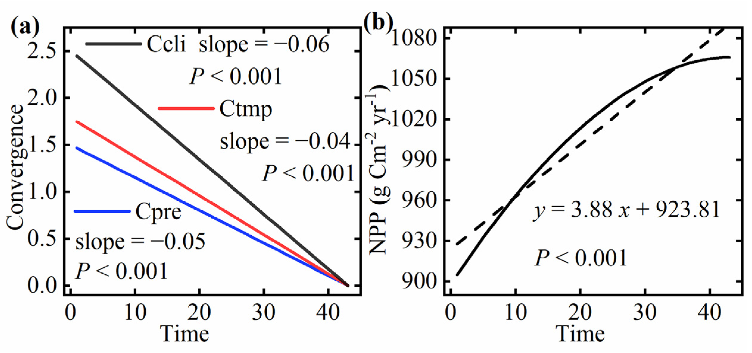
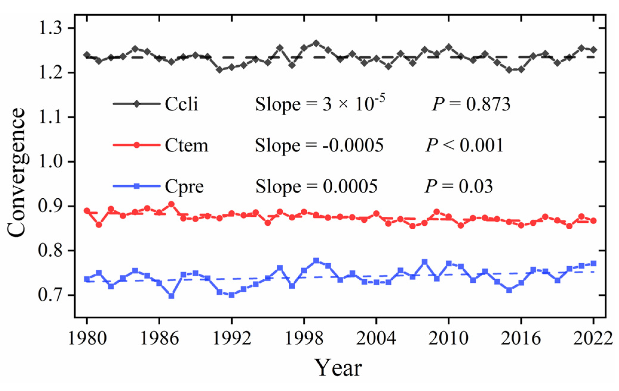
3.1. Trends in Climate Patterns

From 1980 to 2022, both the global average temperature and total precipitation showed fluctuating increasing trends. More than half of the regions experienced an increase in temperature and precipitation, with 81.3% and 57.9% of the areas showing increasing trends in temperature and precipitation, respectively.

Figure 2 illustrates the interannual trends of precipitation, temperature, and climate convergence from 1980 to 2022. Throughout this period, the trend of precipitation convergence shows an upward trend, indicating that the degree of precipitation convergence gradually increases, moving away from the mean. The pattern of precipitation distribution exhibits an imbalance; the convergence of temperature exhibits a highly significant downward trend, meaning the degree of temperature convergence gradually becomes smaller, approaching the mean. The pattern of temperature distribution exhibits a phenomenon of convergence; and the convergence of climate also shows an upward trend, indicating that the degree of climate convergence gradually becomes larger, moving away from the mean. The pattern of climate distribution exhibits an unbalanced phenomenon.

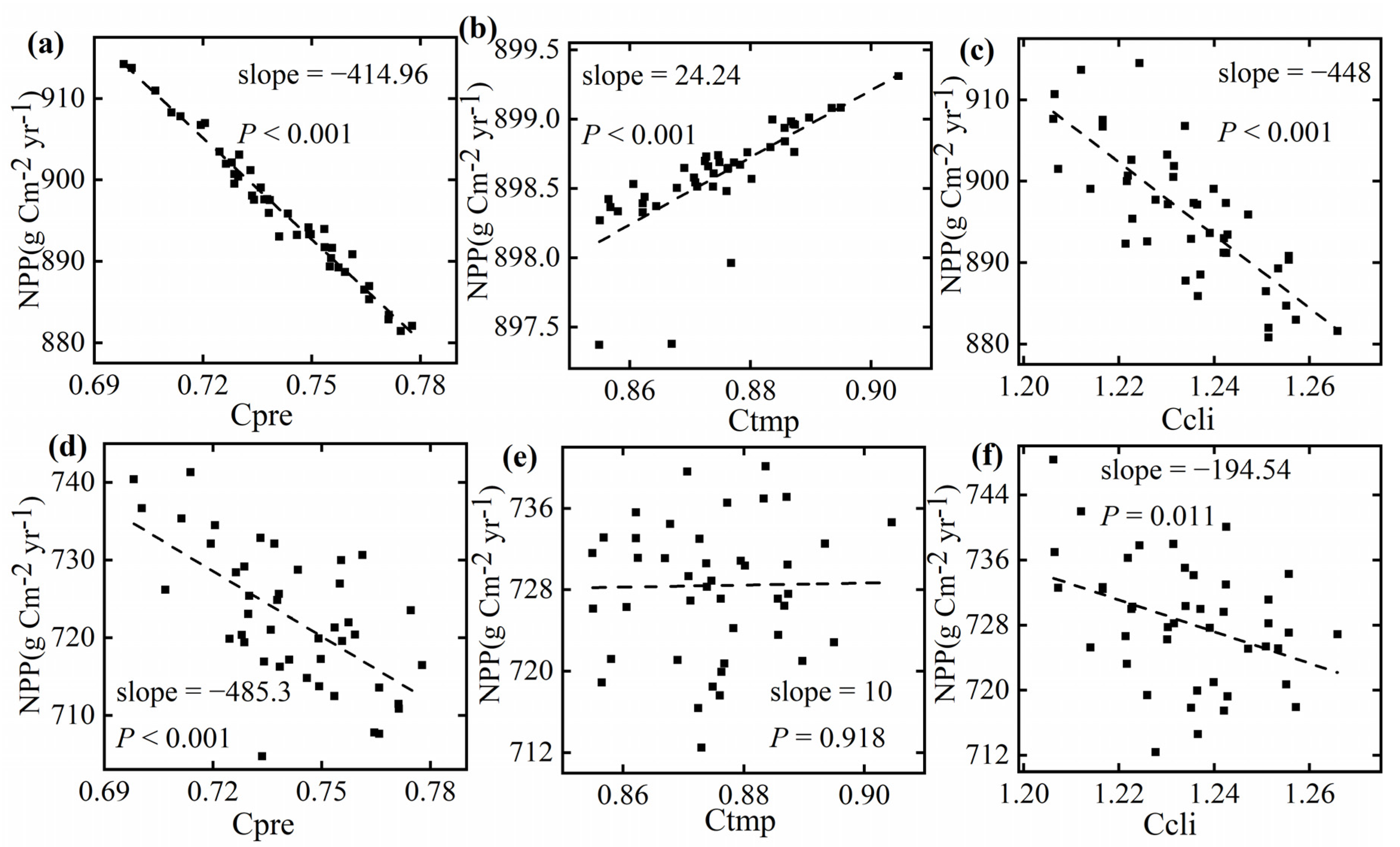
3.2. Climate Patterns Influence Vegetation Productivity

The NPP differences shown in Figure 3a,b are 195 g C m⁻² yr⁻¹ and 167 g C m⁻² yr⁻¹, respectively, which account for 48.6% and 18.4% of the mean NPP values. The NPP in the climate mean zones is significantly higher than the global NPP mean (Figure 3a,b). Moreover, as climate convergence increases, the NPP difference decreases, meaning the global NPP mean becomes larger. The NPP difference estimated using the Thornthwaite model (Figure 3d) shows a significant positive correlation with climate convergence. The difference in NPP calculated from NPP products (Figure 3c) does not show a significant correlation with climate convergence, which may be due to the fact that the NPP in Figure 3c represents actual NPP, influenced by factors such as solar radiation and CO₂.

Although this design idea is quite simple, it initially indicates that vegetation productivity increases when the global climate distribution becomes more uniform (convergence).

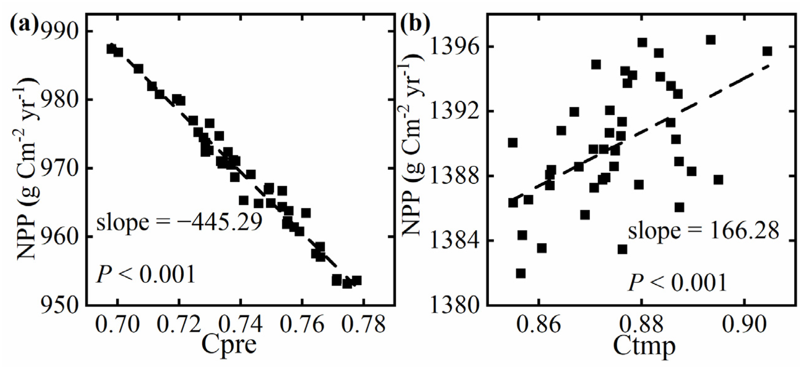
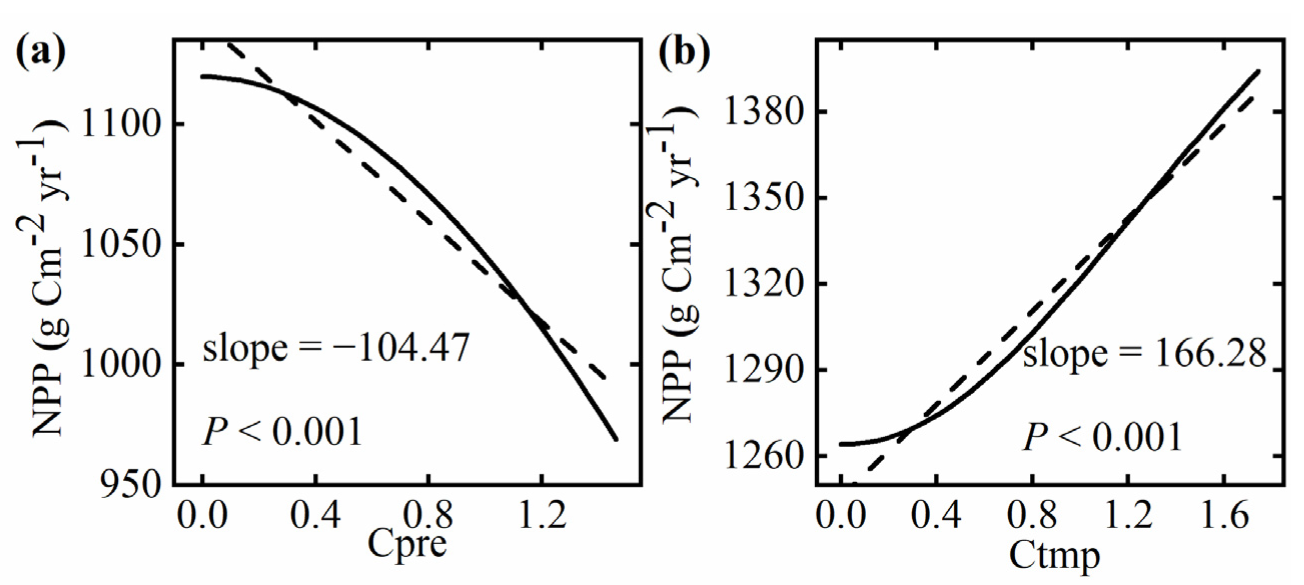
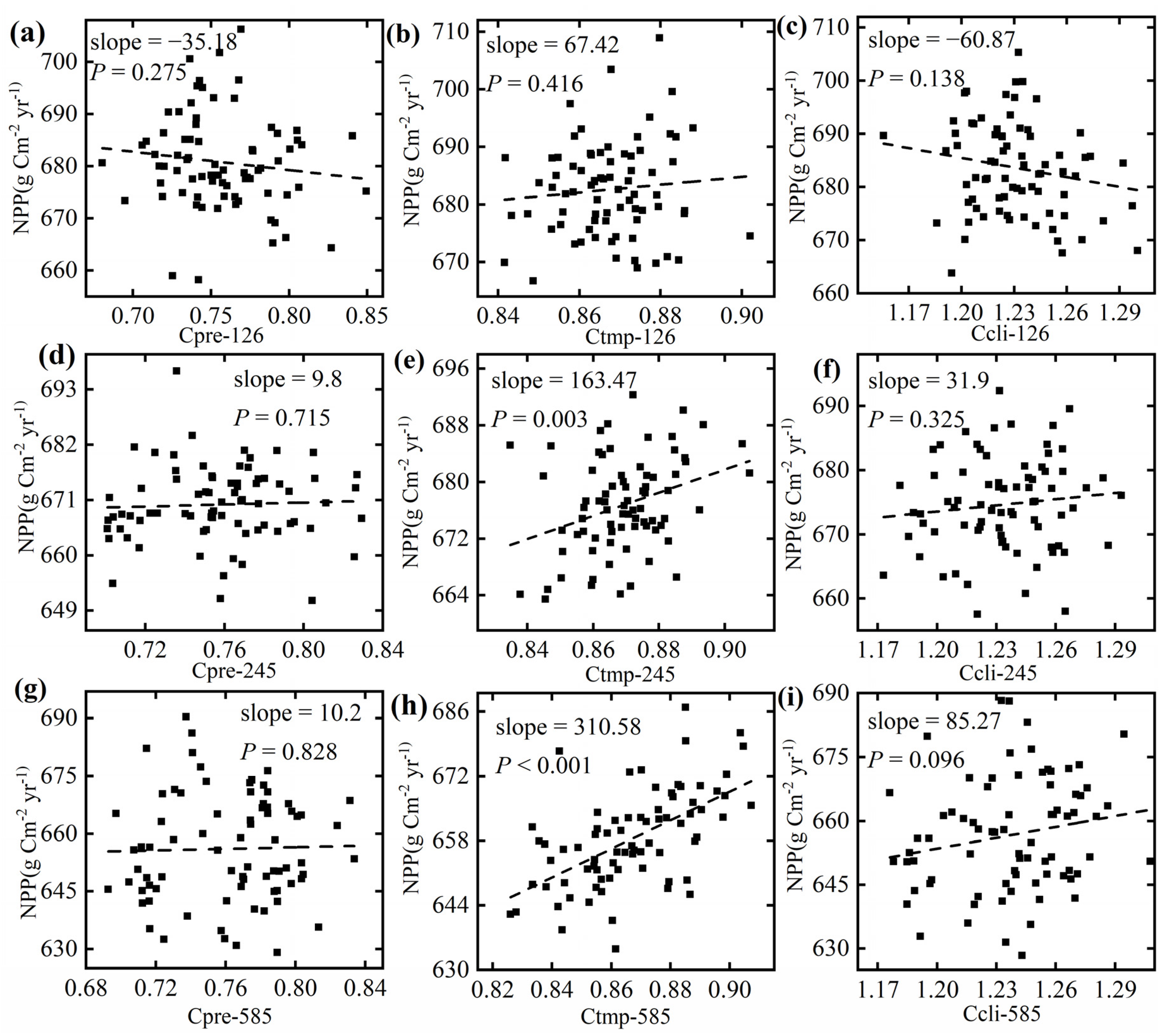
3.3. Relationship Between Climate Pattern and NPP

Between precipitation convergence and NPP are negatively correlated from 1980 to 2022, indicating that as precipitation converges more, NPP significantly increases, with an influence of 35 g C m⁻² yr⁻¹ (Figure 4a). On the other hand, temperature convergence is significantly positively correlated with NPP, indicating that the more the temperature converges, the smaller the NPP. But the impact of temperature convergence is much smaller compared to that of precipitation convergence, with an influence of approximately 1.5 g C m⁻² yr⁻¹ (Figure 4b).

Temperature convergence and precipitation convergence have opposing effects on NPP; however, since precipitation convergence exerts a much greater influence than temperature convergence, the relationship between climate convergence and NPP aligns with the relationship between precipitation convergence and NPP. In other words, as the climate becomes more convergent, NPP significantly increases, with an impact of approximately 30 g C m⁻² yr⁻¹ (Figure 4c). It can be concluded that the influence of climate convergence on NPP from 1980 to 2022 was primarily driven by precipitation. A similar pattern is also observed in the Miami model, as shown in Figure A1.

The relationship between climate patterns and NPP, as derived from the CASA model (Figure 4d–f), exhibits numerical differences when compared to the data in (Figure 4a–c). However, the underlying trends remain consistent, which supports the accuracy of the results presented in Figure 4a–c. There are two primary reasons for these numerical discrepancies: Firstly, there is a disparity in the NPP values estimated by the two models. Secondly, the Thornthwaite model only accounts for the effects of temperature and precipitation, whereas the CASA model incorporates additional influencing factors, including human activities and solar radiation.

The range of convergence changes from 1980 to 2022 is relatively small, which suggests that the relationship between convergence and NPP may not be universal. Therefore, a process was designed in which the convergence gradually decreases from its actual value to zero, and we fit the relationship between convergence and NPP. Using the 1980 temperature and precipitation data, the air temperature and precipitation for each raster were gradually adjusted to approach the complete average distribution over 43 iterations. This process represents a gradual reduction in the convergence of air temperature, precipitation, and climate to zero (Figure A2). Precipitation becomes more convergent, and NPP increases significantly (Figure A3a). The more temperature converges, the more NPP decreases significantly, though the impact is minimal (Figure A3b). The more climate converges, the more NPP increases significantly (Figure A3c). Convergence and NPP follow the same law, as shown in Figure 4, though their numerical values differ. A similar pattern is also observed in the Miami model, as shown in Figure A4.

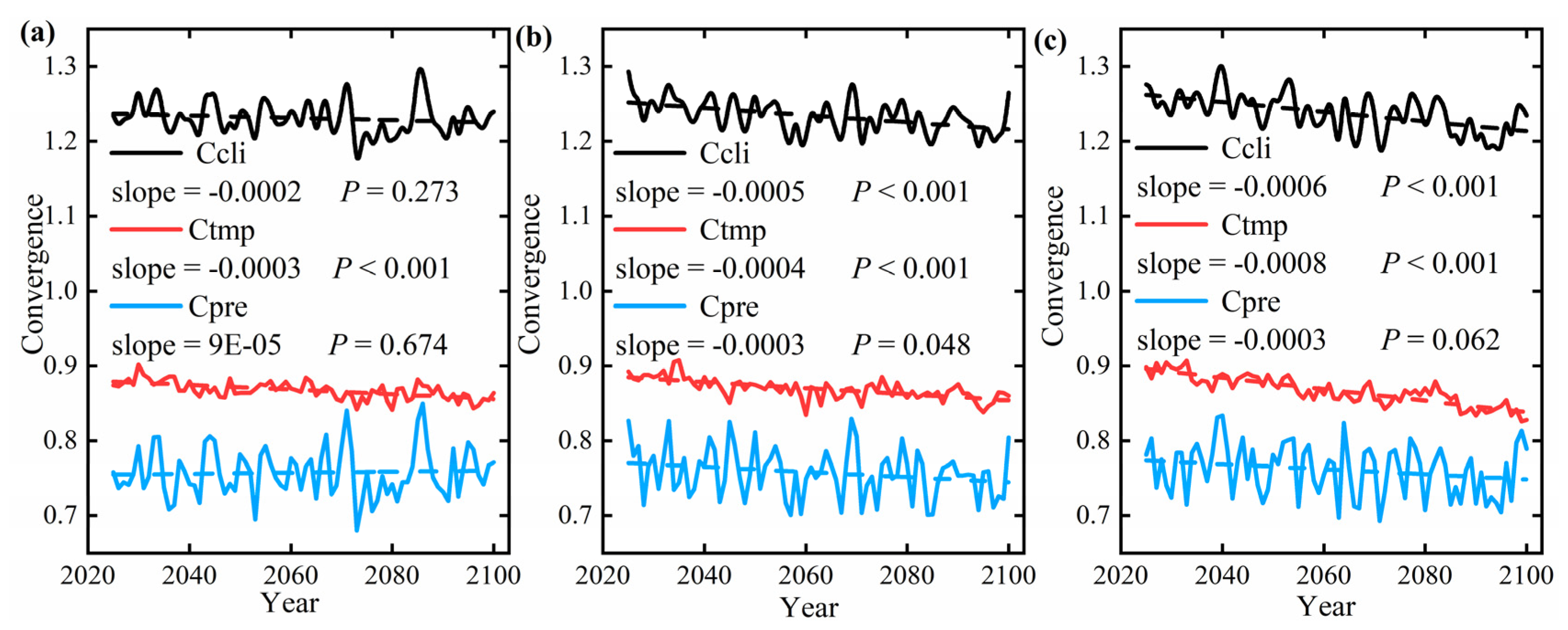
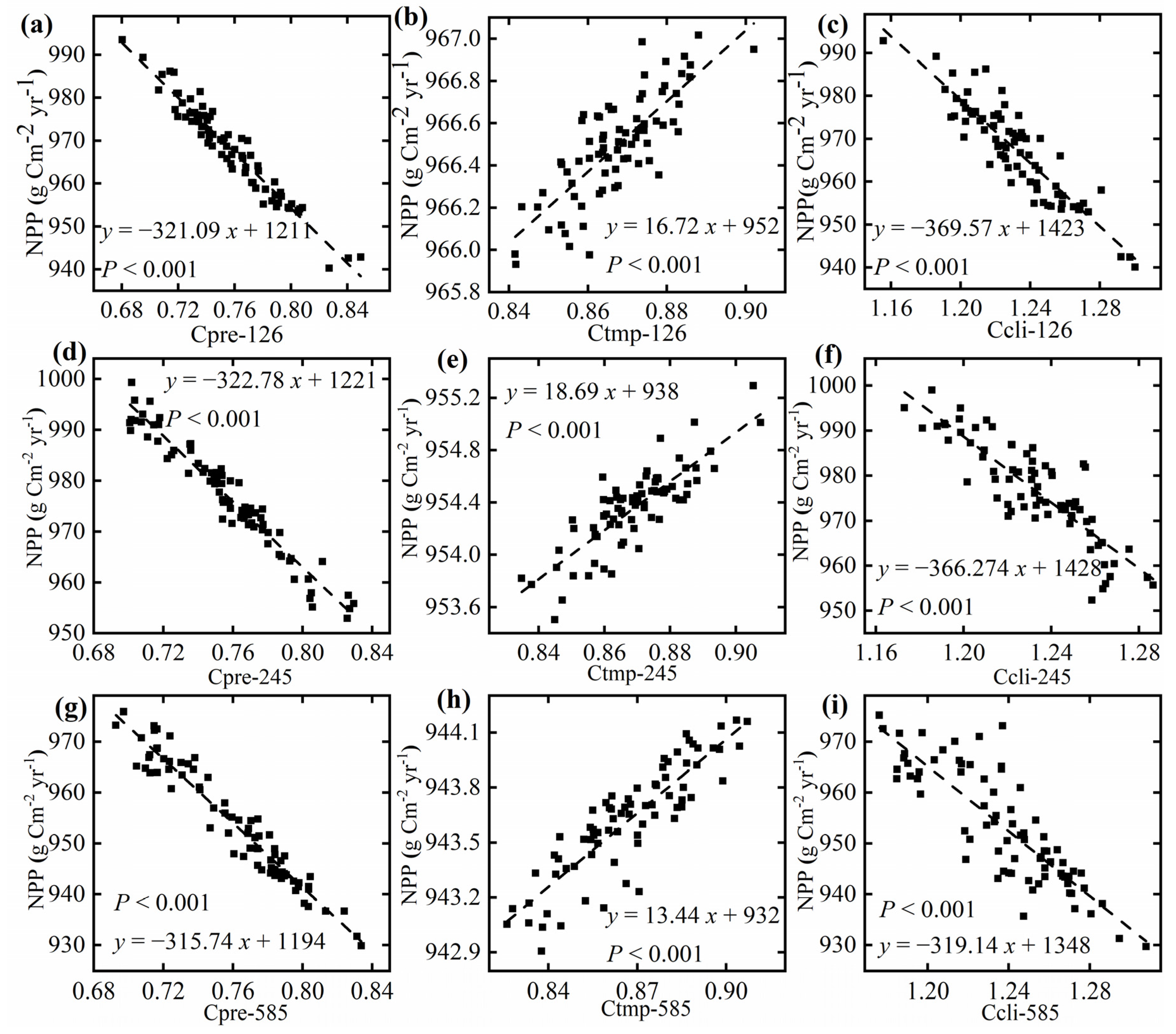
3.4. Impact of Climate Patterns on NPP Under Future Scenarios

Based on the data of 2025, this study investigates the impacts of precipitation convergence, temperature convergence, and climate convergence on NPP across various emission scenarios from 2025 to 2100, employing the methodology used previously. The trends of convergence under the three climate scenarios are detailed in Figure A5. And regarding the relationship between convergence and NPP, the results suggest that the impact of convergence on NPP across the three emission pathways is largely consistent with previous findings for the period 2025–2100. Precipitation convergence is negatively correlated with NPP, with an impact value of approximately 60 g C m⁻² yr⁻¹ (Figure 5a,d,g). In contrast, temperature convergence exhibits a significant positive correlation with NPP, although its impact is considerably less than that of precipitation (Figure 5b,e,h). Since precipitation convergence exerts a greater influence on NPP than temperature convergence, the relationship between climate convergence and NPP aligns with that between precipitation convergence and NNP: there is a significant negative correlation, with an impact value similar to that of precipitation (Figure 5c,f,i). Thus, the relationship between convergence and NPP is stable and independent of emission pathways, although the quantitative relationship between them varies.

Overall, the relationship between NPP simulated by the CASA model and precipitation convergence under future climate scenarios is not significant (Figure 6a,d,g), whereas temperature convergence shows a significant correlation with NPP (Figure 6b,e,h). In the SSP126 scenario, the relationship between NPP simulated by the CASA model and the three-convergence-indices model aligns with that of NPP simulated by the Thornthwaite model. In contrast, under the SSP245 and SSP585 scenarios, the relationship between NPP and temperature convergence simulated by the CASA model is consistent with that simulated by the Thornthwaite model, while the relationship between NPP and precipitation convergence simulated by the CASA model is the inverse of that shown by the Thornthwaite model. Under the SSP245 and SSP585 emission scenarios, the impact of temperature convergence on NPP outweighs that of precipitation convergence. Therefore, the relationship between climate convergence and NPP and temperature convergence is consistent.

4. Discussion

4.1. Mathematical Proof That Climate Convergence Leads to an Increase in NPP

As previously discussed, the influence of climate patterns on vegetation is comprehensive, systematic, and indirect, making it difficult to explain solely through mechanistic models. Therefore, in this study, we intended to provide proof based on mathematical formulae. The mathematical framework assumes that when temperature and precipitation are evenly distributed, there is a high probability that the sum of the products of temperature and precipitation is the maximum. The proof proceeds as follows: The Thornthwaite model is more complex; to simplify the proof, we assume that NPP = T × P. While this assumption does not precisely represent the actual relationship between NPP, temperature, and precipitation, it captures the essence that an increase in both T and P leads to an increase in NPP. The mathematical assumptions are as follows: Let Earth be divided into i raster cells, where T[i] and P[i] represent the temperature and precipitation values for each raster, both of which are greater than 0. The global mean temperature and precipitation are fixed values, denoted as A and B. The task is to find the distribution of T[i] and P[i] when ${\sum }_{\mathrm{i}=1}^{\mathrm{n}}T\left[\mathrm{i}\right]\times P\left[\mathrm{i}\right]$ is the maximum. To solve this problem, we employ Lagrangian multiplication, and begin by constructing the Lagrangian function.

$$\mathbf{f}(\mathbf{T}, \mathbf{P})={\sum }_{\mathbf{i}=1}^{\mathbf{n}}\mathit{T}\left[\mathbf{i}\right]\times \mathit{P}\left[\mathbf{i}\right]-\mathit{\lambda }\left({\sum }_{\mathbf{i}=1}^{\mathbf{n}}\mathit{T}\left[\mathbf{i}\right]-\mathbf{A}\right)-\mathit{\mu }\left({\sum }_{\mathbf{i}=1}^{\mathbf{n}}\mathit{P}\left[\mathbf{i}\right]-\mathbf{B}\right)$$

where λ and µ are Lagrangian multipliers.

We compute the partial derivative of the Lagrange function to T[i] and P[i], and set them to zero:

$${\displaystyle \frac{\mathbf{\partial }\mathbf{f}}{\mathbf{\partial }\mathbf{T}\left[\mathbf{i}\right]}}=\mathit{P}\left[\mathbf{i}\right]-\mathit{\lambda }=0$$

$${\displaystyle \frac{\mathbf{\partial }\mathbf{f}}{\mathbf{\partial }\mathbf{P}\left[\mathbf{i}\right]}}=\mathit{T}\left[\mathbf{i}\right]-\mathit{\mu }=0$$

We obtain

$$\mathit{T}\left[\mathbf{i}\right]=\mathit{\mu }$$

$$\mathit{P}\left[\mathbf{i}\right]=\mathit{\lambda }$$

Substituting the results into the constraints yields

$$\mathit{\mu }\mathit{n}=\mathbf{A}$$

$$\mathit{\lambda }\mathit{n}=\mathbf{B}$$

The solution is $\mu ={\displaystyle \frac{\mathrm{A}}{n}}$, $\lambda ={\displaystyle \frac{\mathrm{B}}{\mathrm{n}}}$, so when T[i] is equal to the mean ${\displaystyle \frac{\mathrm{A}}{n}}$ and P[i] is equal to ${\displaystyle \frac{\mathrm{B}}{\mathrm{n}}}$, the sum of the products is maximized.

4.2. Illustration of Precipitation Convergence Causing an Increase in Global NPP and Temperature Convergence, Resulting in a Decrease in NPP

Theoretically, when the distribution of temperature and precipitation approaches their respective mean values, it can result in an increase in the sum of the products of T[i] and P[i]. This occurs because as the values approach the mean, the probability of the sum of the products reaching the maximum increases, as demonstrated by Lagrangian multiplication. However, this study’s finding that temperature convergence leads to a decrease in NPP seems to contradict the theoretical proof. This discrepancy arises because temperature and precipitation have different levels of significance for NPP. In the theoretical proof, both temperature and precipitation are assumed to be equally important, which does not overturn the above proof.

The primary factors influencing global vegetation productivity are closely related to precipitation [56,57,58,59], a perspective supported by the findings of this study based on actual data. The basic idea includes using the annual global mean temperature and precipitation as benchmarks to classify the world into four climate zones: warm, cold, wet, and dry. The area and the mean of the NPP product of these climate types were statistically analyzed from 1981 to 2019. The results indicate that the mean NPP in wet regions (703 g C m⁻² yr⁻¹) is significantly higher than in dry regions (270 g C m⁻² yr⁻¹), illustrating that precipitation stress is the dominant factor affecting global vegetation productivity. Furthermore, the convergence of precipitation (a more uniform distribution) leads to the expansion of wet areas, which eases moisture stress on vegetation and improves productivity. This increase alleviates the moisture stress of vegetation and improves the productivity of vegetation. In contrast, the average NPP in warm regions (491 g C m⁻² yr⁻¹) is higher than in cold regions (372 g C m⁻² yr⁻¹), suggesting that temperature is also a stress factor for vegetation productivity on a global scale, but the degree of stress is much lower than that of moisture. Although temperature convergence has led to the expansion of warm areas, which may theoretically increase temperature stress, the overall increase in high-temperature stress in warmer regions has been associated with a decrease in global NPP [60,61]. Given that the temperature stress on vegetation is less severe than that caused by precipitation, the impact of temperature convergence on NPP is much smaller compared to that of precipitation convergence.

Overall, while climate convergence has contributed to a decrease in NPP in warmer regions, it has also resulted in a notable increase in NPP in wet areas. Given that the impact of the latter on NPP is much greater than the effect of the former, the net result has been a significant increase in global NPP. This finding further supports the hypothesis that climate convergence leads to an overall enhancement of NPP.

4.3. The Impact of Climate Convergence on Vegetation Productivity Varies Across Different Climate Scenarios

Notably, the relationships between NPP and convergence simulated by the CASA model and the Thornthwaite model align in the historical scenario and the SSP126 scenario, but diverge in SSP245 and SSP585. This consistency in the historical and SSP126 scenarios is due to the fact that the SSP126 scenario represents a low-emission model, where the temperature and precipitation patterns closely resemble those of the historical scenario, resulting in a similar convergence and relationship between NPP and climate. However, the inconsistency in the SSP245 and SSP585 scenarios is attributed to the rapid warming observed under these higher-emission pathways, which drastically alter the state of global climate, with high-temperature stress emerging as the dominant limiting factor for global vegetation [60,61,62,63]. In light of these findings, which model should be considered more reliable in the SSP245 and SSP585 scenarios? This study leans towards the CASA model’s predictions, which suggest that climate convergence leads to a decrease in NPP. There are two main reasons for this preference. Firstly, the Thornthwaite model is an empirical formula tailored to historical climate conditions, making it more applicable to the SSP126 scenario but less suitable for the altered climate states in the SSP245 and SSP585 scenarios. Secondly, the CASA model is a LUE model that integrates temperature and moisture stress factors, providing a more universal framework for estimating vegetation productivity.

5. Conclusions

Studies indicate that precipitation convergence can alleviate global water stress and significantly enhance NPP, whereas temperature convergence intensifies global high-temperature stress, resulting in a reduction in NPP. Considering that the impact of precipitation convergence is greater than that of temperature convergence, it is evident that global climate convergence can substantially increase NPP. Under both the historical and SSP126 scenarios, the relationship between convergence and NPP remains consistent, suggesting that this phenomenon represents a universal law under relatively stable climate conditions. However, this relationship reverses under the SSP245 and SSP585 scenarios, in all three future climate scenarios, the global climate pattern is projected to shift towards greater convergence. Low-emission scenarios favor an increase in vegetation productivity, while high-emission scenarios are not conducive to such growth. The results of this study fill a critical gap in understanding the impact of climate patterns on vegetation productivity. Moreover, if a precise mathematical relationship between climate patterns and vegetation productivity can be established based on this theory, it could greatly simplify global-scale vegetation productivity estimation models. However, this study has some limitations. Firstly, the accuracy of the convergence degree and of the numerical relationship between climate models and NPP requires improvement; secondly, there has been no discussion on the ecological mechanisms behind the impact of climate patterns on NPP based on plant physiology or carbon cycling; additionally, the spatial scale effects of this pattern have not been validated.

References

1. IPCC. Climate Change 2021: The Physical Science Basis. Contribution of Working Group I to the Sixth Assessment Report of the Intergovernmental Panel on Climate Change; Cambridge University Press: Cambridge, UK; New York, NY, USA, 2021. [Google Scholar]
2. Cattiaux, J.; Ribes, A.; Cariou, E. How Extreme Were Daily Global Temperatures in 2023 and Early 2024? Geophys. Res. Lett. 2024, 51, e2024GL110531. [Google Scholar] [CrossRef]
3. Matthews, H.D.; Wynes, S. Current global efforts are insufficient to limit warming to 1.5 °C. Science 2022, 376, 1404–1409. [Google Scholar] [CrossRef] [PubMed]
4. Cohen, J.; Screen, J.A.; Furtado, J.C.; Barlow, M.; Whittleston, D.; Coumou, D.; Francis, J.; Dethloff, K.; Entekhabi, D.; Overland, J.; et al. Recent Arctic amplification and extreme mid-latitude weather. Nat. Geosci. 2014, 7, 627–637. [Google Scholar] [CrossRef]
5. Thorpe, L.; Andrews, T. The physical drivers of historical and 21st century global precipitation changes. Environ. Res. Lett. 2014, 9, 064024. [Google Scholar] [CrossRef]
6. Byrne, M.P.; O’Gorman, P.A. The Response of Precipitation Minus Evapotranspiration to Climate Warming: Why the “Wet-Get-Wetter, Dry-Get-Drier” Scaling Does Not Hold over Land. J. Clim. 2015, 28, 8078–8092. [Google Scholar] [CrossRef]
7. Diffenbaugh, N.S.; Singh, D.; Mankin, J.S.; Horton, D.E.; Swain, D.L.; Touma, D.; Charland, A.; Liu, Y.; Haugen, M.; Tsiang, M.; et al. Quantifying the influence of global warming on unprecedented extreme climate events. Proc. Natl. Acad. Sci. USA 2017, 114, 4881–4886. [Google Scholar] [CrossRef]
8. Trenberth, K.E.; Fasullo, J.T. Tracking Earth’s Energy: From El Niño to Global Warming. Surv. Geophys. 2012, 33, 413–426. [Google Scholar] [CrossRef]
9. Li, C.; Zhou, M.; Dou, T.; Zhu, T.; Yin, H.; Liu, L. Convergence of global hydrothermal pattern leads to an increase in vegetation net primary productivity. Ecol. Indic. 2021, 132, 108282. [Google Scholar] [CrossRef]
10. Liang, Q.; Xu, X.; Mao, K.; Wang, M.; Wang, K.; Xi, Z.; Liu, J. Shifts in plant distributions in response to climate warming in a biodiversity hotspot, the Hengduan Mountains. J. Biogeogr. 2018, 45, 1334–1344. [Google Scholar] [CrossRef]
11. Margalef-Marrase, J.; Pérez-Navarro, M.Á.; Lloret, F. Relationship between heatwave-induced forest die-off and climatic suitability in multiple tree species. Glob. Change Biol. 2020, 26, 3134–3146. [Google Scholar] [CrossRef]
12. Navarro, M.A.P.; Sapes, G.; Batllori, E.; Serra-Diaz, J.M.; Esteve, M.A.; Lloret, F. Climatic Suitability Derived from Species Distribution Models Captures Community Responses to an Extreme Drought Episode. Ecosystems 2019, 22, 77–90. [Google Scholar] [CrossRef]
13. Pan, Y.; Yang, R.; Qiu, J.; Wang, J.; Wu, J. Forty-year spatio-temporal dynamics of agricultural climate suitability in China reveal shifted major crop production areas. CATENA 2023, 226, 107073. [Google Scholar] [CrossRef]
14. Freeman, B.G.; Lee-Yaw, J.A.; Sunday, J.M.; Hargreaves, A.L. Expanding, shifting and shrinking: The impact of global warming on species’ elevational distributions. Glob. Ecol. Biogeogr. 2018, 27, 1268–1276. [Google Scholar] [CrossRef]
15. Suttle, K.B.; Thomsen, M.A.; Power, M.E. Species Interactions Reverse Grassland Responses to Changing Climate. Science 2007, 315, 640–642. [Google Scholar] [CrossRef]
16. Ackerly, D.D.; Kling, M.M.; Clark, M.L.; Papper, P.; Oldfather, M.F.; Flint, A.L.; Flint, L.E. Topoclimates, refugia, and biotic responses to climate change. Front. Ecol. Environ. 2020, 18, 288–297. [Google Scholar] [CrossRef]
17. Hannah, L.; Roehrdanz, P.R.; Ikegami, M.; Shepard, A.V.; Shaw, M.R.; Tabor, G.; Zhi, L.; Marquet, P.A.; Hijmans, R.J. Climate change, wine, and conservation. Proc. Natl. Acad. Sci. USA 2013, 110, 6907–6912. [Google Scholar] [CrossRef]
18. Ashcroft, M.B. Identifying refugia from climate change. J. Biogeogr. 2010, 37, 1407–1413. [Google Scholar] [CrossRef]
19. Gavin, D.G.; Fitzpatrick, M.C.; Gugger, P.F.; Heath, K.D.; Rodríguez-Sánchez, F.; Dobrowski, S.Z.; Hampe, A.; Hu, F.S.; Ashcroft, M.B.; Bartlein, P.J.; et al. Climate refugia: Joint inference from fossil records, species distribution models and phylogeography. New Phytol. 2014, 204, 37–54. [Google Scholar] [CrossRef]
20. Dobrowski, S.Z. A climatic basis for microrefugia: The influence of terrain on climate. Glob. Change Biol. 2011, 17, 1022–1035. [Google Scholar] [CrossRef]
21. Keppel, G.; Van Niel, K.P.; Wardell-Johnson, G.W.; Yates, C.J.; Byrne, M.; Mucina, L.; Schut, A.G.T.; Hopper, S.D.; Franklin, S.E. Refugia: Identifying and understanding safe havens for biodiversity under climate change. Glob. Ecol. Biogeogr. 2012, 21, 393–404. [Google Scholar] [CrossRef]
22. Lenoir, J.; Graae, B.J.; Aarrestad, P.A.; Alsos, I.G.; Armbruster, W.S.; Austrheim, G.; Bergendorff, C.; Birks, H.J.B.; Bråthen, K.A.; Brunet, J.; et al. Local temperatures inferred from plant communities suggest strong spatial buffering of climate warming across Northern Europe. Glob. Change Biol. 2013, 19, 1470–1481. [Google Scholar] [CrossRef]
23. Chen, I.C.; Hill, J.K.; Ohlemüller, R.; Roy, D.B.; Thomas, C.D. Rapid Range Shifts of Species Associated with High Levels of Climate Warming. Science 2011, 333, 1024–1026. [Google Scholar] [CrossRef]
24. Pennington, P.T.; Cronk, Q.C.B.; Richardson, J.A.; Woodward, F.I.; Lomas, M.R.; Kelly, C.K. Global climate and the distribution of plant biomes. Philos. Trans. R. Soc. Lond. Ser. B Biol. Sci. 2004, 359, 1465–1476. [Google Scholar] [CrossRef]
25. Wang, Y.; Pineda-Munoz, S.; McGuire, J.L. Plants maintain climate fidelity in the face of dynamic climate change. Proc. Natl. Acad. Sci. USA 2023, 120, e2201946119. [Google Scholar] [CrossRef]
26. Elser, J.J.; Fagan, W.F.; Kerkhoff, A.J.; Swenson, N.G.; Enquist, B.J. Biological stoichiometry of plant production: Metabolism, scaling and ecological response to global change. New Phytol. 2010, 186, 593–608. [Google Scholar] [CrossRef]
27. Lenoir, J.; Gégout, J.C.; Marquet, P.A.; de Ruffray, P.; Brisse, H. A Significant Upward Shift in Plant Species Optimum Elevation During the 20th Century. Science 2008, 320, 1768–1771. [Google Scholar] [CrossRef]
28. Foley, J.A.; DeFries, R.; Asner, G.P.; Barford, C.; Bonan, G.; Carpenter, S.R.; Chapin, F.S.; Coe, M.T.; Daily, G.C.; Gibbs, H.K.; et al. Global Consequences of Land Use. Science 2005, 309, 570–574. [Google Scholar] [CrossRef]
29. Lambin, E.F.; Meyfroidt, P. Global land use change, economic globalization, and the looming land scarcity. Proc. Natl. Acad. Sci. USA 2011, 108, 3465–3472. [Google Scholar] [CrossRef]
30. Cramer, W.; Bondeau, A.; Woodward, F.I.; Prentice, I.C.; Betts, R.A.; Brovkin, V.; Cox, P.M.; Fisher, V.; Foley, J.A.; Friend, A.D.; et al. Global response of terrestrial ecosystem structure and function to CO2 and climate change: Results from six dynamic global vegetation models. Glob. Change Biol. 2001, 7, 357–373. [Google Scholar] [CrossRef]
31. Kolby Smith, W.; Reed, S.C.; Cleveland, C.C.; Ballantyne, A.P.; Anderegg, W.R.L.; Wieder, W.R.; Liu, Y.Y.; Running, S.W. Large divergence of satellite and Earth system model estimates of global terrestrial CO2 fertilization. Nat. Clim. Change 2016, 6, 306–310. [Google Scholar] [CrossRef]
32. Grimmett, L.; Whitsed, R.; Horta, A. Presence-only species distribution models are sensitive to sample prevalence: Evaluating models using spatial prediction stability and accuracy metrics. Ecol. Modell. 2020, 431, 109194. [Google Scholar] [CrossRef]
33. Nicholson, S. Land surface processes and Sahel climate. Rev. Geophys. 2000, 38, 117–139. [Google Scholar] [CrossRef]
34. Herrmann, S.M.; Anyamba, A.; Tucker, C.J. Recent trends in vegetation dynamics in the African Sahel and their relationship to climate. Glob. Environ. Change 2005, 15, 394–404. [Google Scholar] [CrossRef]
35. Staal, A.; Flores, B.M.; Aguiar, A.P.D.; Bosmans, J.H.C.; Fetzer, I.; Tuinenburg, O.A. Feedback between drought and deforestation in the Amazon. Environ. Res. Lett. 2020, 15, 044024. [Google Scholar] [CrossRef]
36. Berdugo, M.; Gaitán, J.J.; Delgado-Baquerizo, M.; Crowther, T.W.; Dakos, V. Prevalence and drivers of abrupt vegetation shifts in global drylands. Proc. Natl. Acad. Sci. USA 2022, 119, e2123393119. [Google Scholar] [CrossRef]
37. Gong, H.; Wang, G.; Wang, X.; Kuang, Z.; Cheng, T. Trajectories of Terrestrial Vegetation Productivity and Its Driving Factors in China’s Drylands. Geophys. Res. Lett. 2024, 51, e2024GL111391. [Google Scholar] [CrossRef]
38. Guan, Y.; Liu, J.; Cui, W.; Chen, D.; Zhang, J.; Lu, H.; Maeda, E.E.; Zeng, Z.; Beck, H.E. Elevation Regulates the Response of Climate Heterogeneity to Climate Change. Geophys. Res. Lett. 2024, 51, e2024GL109483. [Google Scholar] [CrossRef]
39. Zhong, Z.; He, B.; Wang, Y.-P.; Chen, H.W.; Chen, D.; Fu, Y.H.; Chen, Y.; Guo, L.; Deng, Y.; Huang, L.; et al. Disentangling the effects of vapor pressure deficit on northern terrestrial vegetation productivity. Sci. Adv. 2023, 9, eadf3166. [Google Scholar] [CrossRef]
40. Grace, J.B.; Anderson, T.M.; Seabloom, E.W.; Borer, E.T.; Adler, P.B.; Harpole, W.S.; Hautier, Y.; Hillebrand, H.; Lind, E.M.; Pärtel, M.; et al. Integrative modelling reveals mechanisms linking productivity and plant species richness. Nature 2016, 529, 390–393. [Google Scholar] [CrossRef] [PubMed]
41. Li, C.; Liu, C.; Tsunekawa, A.; Liu, Y.; Yin, P.; Ma, S.; Zhou, M.; Wu, X. Climate Change Is Leading to a Convergence of Global Climate Distribution. Geophys. Res. Lett. 2024, 51, e2023GL106658. [Google Scholar] [CrossRef]
42. Trenberth, K.E.; Fasullo, J.T. Climate extremes and climate change: The Russian heat wave and other climate extremes of 2010. J. Geophys. Res. Atmos. 2012, 117, D17103. [Google Scholar] [CrossRef]
43. Donat, M.G.; Lowry, A.L.; Alexander, L.V.; O’Gorman, P.A.; Maher, N. More extreme precipitation in the world’s dry and wet regions. Nat. Clim. Change 2016, 6, 508–513. [Google Scholar] [CrossRef]
44. Keppel, G.; Wardell-Johnson, G.W. Refugia: Keys to climate change management. Glob. Change Biol. 2012, 18, 2389–2391. [Google Scholar] [CrossRef]
45. Thornthwaite, C.W. An Approach Toward a Rational Classification of Climate. Soil Sci. 1948, 66, 55–94. [Google Scholar] [CrossRef]
46. Running, S.W.; Coughlan, J.C. A general model of forest ecosystem processes for regional applications I. Hydrologic balance, canopy gas exchange and primary production processes. Ecol. Modell. 1988, 42, 125–154. [Google Scholar] [CrossRef]
47. Harris, I.; Jones, P.; Osborn, T.; Lister, D. Updated high-resolution grids of monthly climatic observations-the CRU TS3. 10 Dataset. Int. J. Climatol. 2014, 34, 623–642. [Google Scholar] [CrossRef]
48. Peng, S.; Piao, S.; Ciais, P.; Myneni, R.B.; Chen, A.; Chevallier, F.; Dolman, A.J.; Janssens, I.A.; Penuelas, J.; Zhang, G. Asymmetric effects of daytime and night-time warming on Northern Hemisphere vegetation. Nature 2013, 501, 88–92. [Google Scholar] [CrossRef]
49. Zhang, L.; Chen, X.; Xin, X. Short Commentary on CMIP6 Scenario Model Intercomparison Project (ScenarioMIP). Clim. Change Res. 2019, 15, 519–525. [Google Scholar]
50. Du, Y.; Wang, D.; Zhu, J.; Wang, D.; Qi, X.; Cai, J. Comprehensive assessment of CMIP5 and CMIP6 models in simulating and projecting precipitation over the global land. Int. J. Climatol. 2022, 42, 6859–6875. [Google Scholar] [CrossRef]
51. Zhu, Y.-Y.; Yang, S. Evaluation of CMIP6 for historical temperature and precipitation over the Tibetan Plateau and its comparison with CMIP5. Adv. Clim. Change Res. 2020, 11, 239–251. [Google Scholar] [CrossRef]
52. Chen, J.M.; Ju, W.; Ciais, P.; Viovy, N.; Liu, R.; Liu, Y.; Lu, X. Vegetation structural change since 1981 significantly enhanced the terrestrial carbon sink. Nat. Commun. 2019, 10, 4259. [Google Scholar] [CrossRef]
53. Liu, Y.; Zhou, Y.; Ju, W.; Wang, S.; Wu, X.; He, M.; Zhu, G. Impacts of droughts on carbon sequestration by China’s terrestrial ecosystems from 2000 to 2011. Biogeosciences 2014, 11, 2583–2599. [Google Scholar] [CrossRef]
54. Lieth, H. Modeling the primary productivity of the world. In Primary Productivity of the Biosphere; Springer: Berlin/Heidelberg, Germany, 1975; pp. 237–263. [Google Scholar] [CrossRef]
55. Potter, C.S.; Randerson, J.T.; Field, C.B.; Matson, P.A.; Vitousek, P.M.; Mooney, H.A.; Klooster, S.A. Terrestrial ecosystem production: A process model based on global satellite and surface data. Glob. Biogeochem. Cycles 1993, 7, 811–841. [Google Scholar] [CrossRef]
56. Liu, M.; Wang, H.; Zhai, H.; Zhang, X.; Shakir, M.; Ma, J.; Sun, W. Identifying thresholds of time-lag and accumulative effects of extreme precipitation on major vegetation types at global scale. Agric. For. Meteorol. 2024, 358, 110239. [Google Scholar] [CrossRef]
57. Zeng, X.; Hu, Z.; Chen, A.; Yuan, W.; Hou, G.; Han, D.; Liang, M.; Di, K.; Cao, R.; Luo, D. The global decline in the sensitivity of vegetation productivity to precipitation from 2001 to 2018. Glob. Change Biol. 2022, 28, 6823–6833. [Google Scholar] [CrossRef]
58. Berdugo, M.; Delgado-Baquerizo, M.; Soliveres, S.; Hernández-Clemente, R.; Zhao, Y.; Gaitán, J.J.; Gross, N.; Saiz, H.; Maire, V.; Lehmann, A. Global ecosystem thresholds driven by aridity. Science 2020, 367, 787–790. [Google Scholar] [CrossRef]
59. Guan, K.; Pan, M.; Li, H.; Wolf, A.; Wu, J.; Medvigy, D.; Caylor, K.K.; Sheffield, J.; Wood, E.F.; Malhi, Y. Photosynthetic seasonality of global tropical forests constrained by hydroclimate. Nat. Geosci. 2015, 8, 284–289. [Google Scholar] [CrossRef]
60. Li, X.; Huntingford, C.; Wang, K.; Cui, J.; Xu, H.; Kan, F.; Anniwaer, N.; Yang, H.; Peñuelas, J.; Piao, S. Increased crossing of thermal stress thresholds of vegetation under global warming. Glob. Change Biol. 2024, 30, e17406. [Google Scholar] [CrossRef]
61. Williams, I.N.; Torn, M.S.; Riley, W.J.; Wehner, M.F. Impacts of climate extremes on gross primary production under global warming. Environ. Res. Lett. 2014, 9, 094011. [Google Scholar] [CrossRef]
62. Yuxi, W.; Li, P.; Yuemin, Y.; Tiantian, C. Global Vegetation-Temperature Sensitivity and Its Driving Forces in the 21st Century. Earth’s Future 2024, 12, e2022EF003395. [Google Scholar] [CrossRef]
63. Yang, H.; Zhong, C.; Jin, T.; Chen, J.; Zhang, Z.; Hu, Z.; Wu, K. Stronger Impact of Extreme Heat Event on Vegetation Temperature Sensitivity under Future Scenarios with High-Emission Intensity. Remote Sens. 2024, 16, 3708. [Google Scholar] [CrossRef]
64. Harris, I.; Osborn, T.J.; Jones, P.; Lister, D. Version 4 of the CRU TS monthly high-resolution gridded multivariate climate dataset. Sci. Data 2020, 7, 109. [Google Scholar] [CrossRef]
65. Dix, M.; Bi, D.; Dobrohotoff, P.; Fiedler, R.; Harman, I.; Law, R.; Mackallah, C.; Marsland, S.; O’Farrell, S.; Rashid, H.; et al. CSIRO-ARCCSS ACCESS-CM2 Model Output Prepared for CMIP6 ScenarioMIP ssp126; Earth System Grid Federation: Online, 2019. [Google Scholar] [CrossRef]
66. Seland, Ø.; Bentsen, M.; Oliviè, D.J.L.; Toniazzo, T.; Gjermundsen, A.; Graff, L.S.; Debernard, J.B.; Gupta, A.K.; He, Y.; Kirkevåg, A.; et al. NCC NorESM2-LM Model Output Prepared for CMIP6 ScenarioMIP ssp126; Earth System Grid Federation: Online, 2019. [Google Scholar] [CrossRef]
67. Dix, M.; Bi, D.; Dobrohotoff, P.; Fiedler, R.; Harman, I.; Law, R.; Mackallah, C.; Marsland, S.; O’Farrell, S.; Rashid, H.; et al. CSIRO-ARCCSS ACCESS-CM2 Model Output Prepared for CMIP6 ScenarioMIP ssp245; Earth System Grid Federation: Online, 2019. [Google Scholar] [CrossRef]
68. Seland, Ø.; Bentsen, M.; Oliviè, D.J.L.; Toniazzo, T.; Gjermundsen, A.; Graff, L.S.; Debernard, J.B.; Gupta, A.K.; He, Y.; Kirkevåg, A.; et al. NCC NorESM2-LM Model Output Prepared for CMIP6 DAMIP ssp245-aer; Earth System Grid Federation: Online, 2021. [Google Scholar] [CrossRef]
69. Dix, M.; Bi, D.; Dobrohotoff, P.; Fiedler, R.; Harman, I.; Law, R.; Mackallah, C.; Marsland, S.; O’Farrell, S.; Rashid, H.; et al. CSIRO-ARCCSS ACCESS-CM2 Model Output Prepared for CMIP6 ScenarioMIP ssp585; Earth System Grid Federation: Online, 2019. [Google Scholar] [CrossRef]
70. Schwinger, J.; Tjiputra, J.; Seland, Ø.; Bentsen, M.; Oliviè, D.J.L.; Toniazzo, T.; Gjermundsen, A.; Graff, L.S.; Debernard, J.B.; Gupta, A.K.; et al. NCC NorESM2-LM Model Output Prepared for CMIP6 C4MIP esm-ssp585; Earth System Grid Federation: Online, 2020. [Google Scholar] [CrossRef]
Figure 1. Research Flowchart.
Land 14 00570 g001
Figure 2. Trends in Cpre, Ctem, and Ccli from 1980 to 2022.
Land 14 00570 g002
Figure 3. The relationship between the climate mean region NPP and the mean global NPP and the difference between them, and the convergence from 1981 to 2019. Figure (a,b) show the climate mean region NPP (red line) and the global NPP mean (black line)—(a): the NPP product; (b): the Thornthwaite model estimate. Figure (c) illustrates the relationship between the difference in NPP products and climate convergence; Figure (d) depicts the relationship between the difference in NPP estimated by the Thornthwaite model and climate convergence.
Land 14 00570 g003
Figure 4. The relationship between precipitation convergence, temperature convergence, climate convergence, and NPP from 1980 to 2022. The NPP in Figure (a,d): temperature data from 1980; precipitation data from 1980 to 2022, with each year’s average precipitation being equal to that of 1980. The NPP in Figure (b,e): precipitation data from 1980; temperature data from 1980 to 2022, with each year’s average temperature being equal to that of 1980. The NPP in Figure (c,f): temperature data from 1980 to 2022, with each year’s average temperature being equal to that of 1980; precipitation data from 1980 to 2022, with each year’s average precipitation being equal to that of 1980. The NPP values in Figure (ac) are the result of the Thornthwaite model calculation, and the NPP values in Figure (df) are the result of the CASA model calculation.
Land 14 00570 g004
Figure 5. Relationship between global Cpre, Ctmp, Ccli, and NPP under SSP126 (ac), SSP245 (df), and SSP585 (gi) from 2025 to 2100. NPP is calculated using the Thornthwaite model.
Land 14 00570 g005
Figure 6. Relationship between global Cpre, Ctmp, and Ccli, and NPP under SSP126 (ac), SSP245 (df), and SSP585 (gi) from 2025 to 2100. NPP is calculated using the CASA model.
Land 14 00570 g006
Disclaimer/Publisher’s Note: The statements, opinions and data contained in all publications are solely those of the individual author(s) and contributor(s) and not of MDPI and/or the editor(s). MDPI and/or the editor(s) disclaim responsibility for any injury to people or property resulting from any ideas, methods, instructions or products referred to in the content.