Article

Landslide Susceptibility Mapping in Xinjiang: Identifying Critical Thresholds and Interaction Effects Among Disaster-Causing Factors

1
School of Public Policy and Management, China University of Mining and Technology, Xuzhou 221116, China
2
Xinjiang Power Transmission and Transformation Co., Ltd., Urumqi 830000, China
3
Zhongdihuaan Science and Technology Co., Ltd., Urumqi 830000, China
*
Author to whom correspondence should be addressed.
Present address: Room A512, School of Public Policy & Management School of Emergency Management, China University of Mining and Technology, No.1 Daxue Street, Tongshan District, Xuzhou 221116, China.
Land 2025, 14(3), 555; https://doi.org/10.3390/land14030555
Submission received: 21 January 2025 / Revised: 22 February 2025 / Accepted: 4 March 2025 / Published: 6 March 2025

Abstract

:
Landslides frequently occur in the Xinjiang Uygur Autonomous Region of China due to its complex geological environment, posing serious risks to human safety and economic stability. Existing studies widely use machine learning models for landslide susceptibility prediction. However, they often fail to capture the threshold and interaction effects among environmental factors, limiting their ability to accurately identify high-risk zones. To address this gap, this study employed a gradient boosting decision tree (GBDT) model to identify critical thresholds and interaction effects among disaster-causing factors, while mapping the spatial distribution of landslide susceptibility based on 20 covariates. The performance of this model was compared with that of a support vector machine and deep neural network models. Results showed that the GBDT model achieved superior performance, with the highest AUC and recall values among the tested models. After applying clustering algorithms for non-landslide sample selection, the GBDT model maintained a high recall value of 0.963, demonstrating its robustness against imbalanced datasets. The GBDT model identified that 8.86% of Xinjiang’s total area exhibits extremely high or high landslide susceptibility, mainly concentrated in the Tianshan and Altai mountain ranges. Lithology, precipitation, profile curvature, the Modified Normalized Difference Water Index (MNDWI), and vertical deformation were identified as the primary contributing factors. Threshold effects were observed in the relationships between these factors and landslide susceptibility. The probability of landslide occurrence increased sharply when precipitation exceeded 2500 mm, vertical deformation was greater than 0 mm a−1, or the MNDWI values were extreme (<−0.4, >0.2). Additionally, this study confirmed bivariate interaction effects. Most interactions between factors exhibited positive effects, suggesting that combining two factors enhances classification performance compared with using each factor independently. This finding highlights the intricate and interdependent nature of these factors in landslide susceptibility. These findings emphasize the necessity of incorporating threshold and interaction effects in landslide susceptibility assessments, offering practical insights for disaster prevention and mitigation.

1. Introduction

Landslides are among the most frequent and devastating geological hazards worldwide, posing severe threats to infrastructure, economic stability, and human safety [1,2,3,4,5,6]. In China, the Xinjiang Uygur Autonomous Region, located at the intersection of the Eurasian and Indian Ocean tectonic plates, near the Himalayan volcanic-seismic belt, is particularly prone to landslides because of its complex geological conditions. This unique setting contributes to frequent geological disasters. By the end of 2021, Xinjiang had identified 2278 potential landslide hazard points, threatening approximately 53,400 people and property worth 2.916 billion CNY [7]. Landslide susceptibility mapping (LSM) is a critical first step in landslide mitigation strategies [8,9,10]. Accurately assessing landslide susceptibility is essential for understanding landslide formation mechanisms, predicting potential landslide locations, and formulating effective disaster mitigation strategies [11,12].
LSM plays a fundamental role in disaster prevention, offering insights into high-risk areas and guiding land-use planning [13,14]. Traditionally, LSM approaches fall into two categories: qualitative and quantitative. Qualitative methods primarily rely on expert knowledge, leading to subjectivity and inconsistencies [15,16]. Conversely, quantitative methods, particularly those utilizing machine learning (ML), have demonstrated remarkable advantages in capturing the nonlinear relationships between landslides and environmental factors [17,18,19,20]. For instance, Wang et al. [21] applied a convolutional neural network (CNN) model for LSM in Qianshan County, demonstrating the potential of CNNs in this field. Similarly, Wu et al. [22] employed a random forest model to assess landslide susceptibility in the Hubei section of the Three Gorges Reservoir Area, highlighting its strong spatial prediction capabilities. Abbas et al. [23] integrated Bayesian and metaheuristic algorithms to optimize feature selection in artificial neural networks (ANNs) for landslide susceptibility analysis. Zhou et al. [24] demonstrated the superior performance of the support vector machine model through a comparison with logistic regression and ANN models.
Despite the remarkable predictive power of ML models, their “black-box” nature limits interpretability, so understanding the underlying mechanisms governing landslides is challenging. One critical limitation is the insufficient consideration of threshold effects and interaction effects among environmental factors. Threshold effects refer to abrupt changes in landslide susceptibility when a specific factor surpasses a critical value [25,26,27,28]. The existing research has largely explored threshold effects based on landslide-triggering conditions. For instance, Avcı et al. [29] observed that precipitation does not have a linear effect on landslides; landslide risk surges once precipitation exceeds a threshold (e.g., 160 mm/day). Similarly, Li et al. [30] found that landslide risk is negligible in areas where Newmark displacement (the cumulative displacement of a landslide mass under seismic forces) is below 10. However, when Newmark displacement exceeds 10, landslide probability increases sharply. Despite these insights, the threshold effects of other environmental factors remain underexplored. Factors such as the Modified Normalized Difference Water Index (MNDWI), distance to rivers (Dis_river), distance to roads (Dis_road), surface elevation (SE), vertical deformation, and distance to faults (Dis_fault) require further investigation. Researching these threshold effects is critical for improving the accuracy and comprehensiveness of landslide susceptibility models.
Moreover, landslide susceptibility is rarely influenced by a single factor; instead, interaction effects between variables play a critical role. For example, Zhang et al. [31] discovered that the intensity of landslides on slopes of the same gradient varies depending on land use, indicating the interplay between slope and land use. Additionally, Abbas et al. [32] revealed that land use significantly weakens the influence of distance to water sources on landslide susceptibility when these two factors act in combination. However, most ML-based LSM studies treat environmental factors as independent variables, failing to account for their combined effects, thereby limiting predictive accuracy.
To address these challenges, this study employs a gradient boosting decision tree (GBDT) model integrated with partial dependence plots (PDPs) to analyze threshold and interaction effects in landslide susceptibility. The GBDT, an ensemble learning method, excels in capturing complex nonlinear relationships, whereas PDPs provide visual insights into the marginal effects of independent variables on landslide susceptibility [33]. By leveraging these methods, this study aims to identify the primary environmental factors influencing landslide susceptibility in Xinjiang. This study seeks to quantify the threshold effects of key variables and determine critical tipping points for landslide occurrence. It also investigates interaction effects among environmental factors to improve the interpretability of landslide susceptibility models. Furthermore, a high-resolution landslide susceptibility map is generated to facilitate risk assessment and disaster mitigation efforts. The findings contribute to an interpretable and reliable landslide susceptibility assessment, providing valuable insights for policymakers and disaster management agencies.

2. Materials and Methods

2.1. Study Area

Located in the heart of the Asian continent (73.0° E–96.3° E, 34.1° N–49.2° N), Xinjiang is characterized by a complex topography dominated by the Altai Mountains in the north, the Tianshan Mountains in the center, and the Kunlun Mountains in the south (Figure 1). The Junggar and Tarim Basins are situated between them. The region lies within a tectonically active zone with well-developed fault structures, including the Tarim, Tianshan, Junggar, and Altai Blocks, which contribute to frequent geological hazards, particularly landslides. The geological composition consists mainly of Paleozoic and Mesozoic sedimentary, metamorphic, and volcanic rocks, further exacerbating landslide susceptibility. Additionally, seismic activity along the Tianshan and Kunlun Mountain belts increases the risk of geological movements. Given the high frequency of landslides in the region, a comprehensive assessment of landslide susceptibility is crucial for disaster prevention and mitigation [34].

2.2. Data Collection and Preprocessing

2.2.1. Acquisition and Processing of Landslide Points

Landslide data were obtained from the Global Disaster Data Platform (https://www.gddat.cn/, accessed on 25 February 2025) and the Resource and Environment Science and Data Center of the Chinese Academy of Sciences (https://www.resdc.cn/, accessed on 25 February 2025). These datasets were cross-verified, resulting in the selection of 1000 landslide points to create a geospatial database of landslide occurrences.
LSM is treated as a binary classification problem. Therefore, non-landslide samples must be generated [35,36]. Xinjiang contains vast desert areas, so the landslide datasets primarily covered populated regions, excluding uninhabited zones. Consequently, when selecting non-landslide samples, areas classified as uninhabited zones in Xinjiang were excluded. A random sampling strategy was employed to generate non-landslide points at a 1:6 ratio, creating a geospatial database of non-landslide occurrences.

2.2.2. Acquisition and Processing of Possible Landslide Conditioning Factors (LCFs)

In this study, we considered internal and external factors to construct an evaluation framework. We selected six primary indicators—topography, geology, hydrology, human activities, land cover, and other factors—and incorporated twenty secondary indicators associated with these primary factors. These indicators form the potential influencing factors, as shown in Table 1.
The data used in this study were derived from various sources to ensure accuracy and reliability. Elevation data were obtained from the Geospatial Data Cloud (https://www.gscloud.cn/, accessed on 25 February 2025). The slope, profile curvature (Figure 2c), Topographic Wetness Index (TWI) (Figure 2j), Topographic Roughness Index (TRI), and aspect data were calculated from elevation data using the ArcGIS platform. Data on landforms were downloaded from the Institute of Geographic Sciences and Natural Resources Research, Chinese Academy of Sciences (https://www.resdc.cn/, accessed on 25 February 2025). Depth to bedrock was sourced from the ISRIC database (https://www.isric.org/, accessed on 25 February 2025). Lithology (Figure 2a) and landcover (Figure 2g) were obtained from the USGS Earth Science and Environmental Change Science Center (https://www.usgs.gov/, accessed on 25 February 2025). Data on faults (Figure 2h) came from the 1:2,500,000 scale Digital Geological Map of the People’s Republic of China, available from the Geological Science Data Publishing System (http://dcc.ngac.org.cn/, accessed on 25 February 2025). River (Figure 2l) and road (Figure 2i) data were retrieved from OpenStreetMap (https://www.openstreetmap.org/, accessed on 25 February 2025). Mining (Figure 2k) data were sourced from the Global Disaster Database (https://www.gddat.cn/, accessed on 25 February 2025). Fault, river, road, and mining data were imported into ArcGIS10.8, where Euclidean distance tools were used to generate distance raster layers. Prep (Figure 2b) was downloaded from the PANGAEA Data Publisher (https://doi.pangaea.de/, accessed on 25 February 2025) and used to calculate the maximum daily precipitation for each raster using the Python3.12 platform. The Normalized Difference Bare and Built-up Index (NDBBI) [37], the MNDWI (Figure 2d) [38], and the Normalized Difference Vegetation Index (NDVI) were calculated using Landsat 8 remote sensing imagery on the Google Earth Engine platform. The annual maximum NDVI, the average NDBBI, and the MNDWI from 2013 to 2019 were derived. Vertical_deformation (Figure 2e) was downloaded from the National Earth System Science Data Center (http://www.geodata.cn, accessed on 25 February 2025) and converted from point data to raster format using ArcGIS. Soil erosion (SE) (Figure 2f) [39] was obtained from the Zenodo database (https://zenodo.org/, accessed on 25 February 2025).

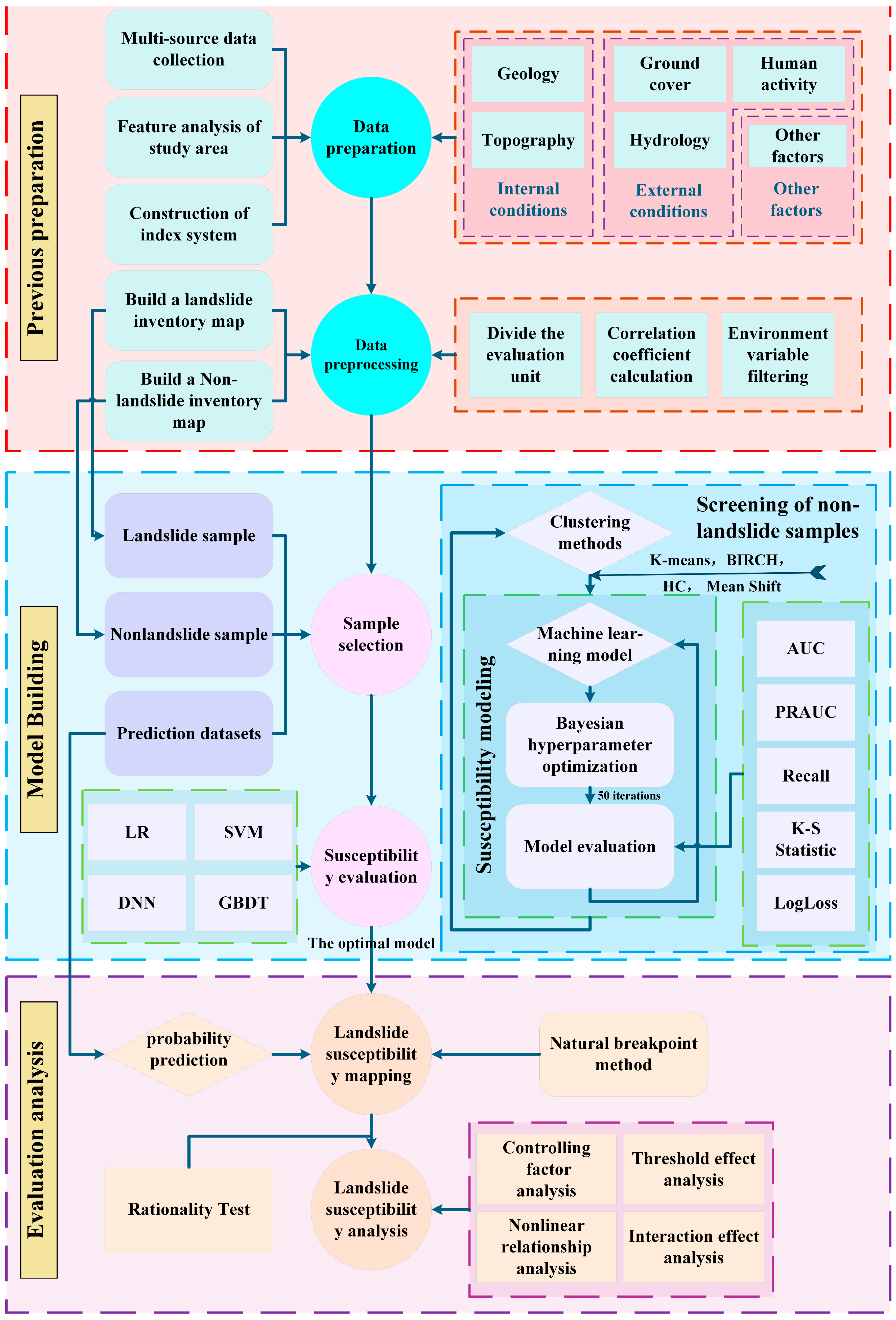
2.3. Technical Workflow of LSM

In geological hazard assessment, ensuring consistency within and between evaluation units is crucial [40]. Therefore, this study resampled all input data to a unified spatial resolution of 30 m to maintain data consistency and ensured that the model can capture fine-scale spatial patterns. Landslide and non-landslide points were labeled as 1 and 0, respectively [41,42], as the response variable for model training. A total of 20 landslide conditioning factors (LCFs), covering terrain, geology, hydrology, and human influence, were extracted to construct the modeling dataset.
Before modeling, feature selection was performed using Spearman’s rank correlation coefficient. Landslide occurrence is often influenced by threshold effects, interactions, geological complexity, and cumulative effects, making the relationship with hazard factors nonlinear and difficult to accurately describe with simple linear models. Spearman’s correlation coefficient is particularly suited for landslide susceptibility assessments. It captures nonlinear relationships between LCFs, offering greater applicability than Pearson’s correlation coefficient, which measures only linear correlations. This study removed factors with a correlation coefficient greater than 0.5 to reduce multicollinearity [43,44], thereby enhancing the model’s stability and interpretability [41,42].
To reduce bias in the LSM, generating high-quality non-landslide samples is essential [45]. Previous studies have shown that clustering methods can effectively select non-landslide sample points, confirming their feasibility [35,46]. Therefore, this study used four clustering methods—k-means, HC, BIRCH, and mean shift—to ensure that non-landslide sample points are distributed in geologically stable regions with clear environmental characteristics. These methods were selected based on their different clustering mechanisms. K-means is centroid-based, HC uses a hierarchical structure, BIRCH is optimized for large datasets, and mean shift is density-based, optimizing sample selection from different perspectives [36,47].
This study defines LSM as a binary classification problem and compares four machine learning models: LR, SVM, DNN, and GBDT. To optimize model performance, Bayesian optimization is used for hyperparameter tuning to efficiently search the hyperparameter space while maximizing the AUC [48]. Compared with grid search or random search, Bayesian optimization iteratively optimizes results based on previous search results, converging to the optimal parameter configuration more quickly. Considering diminishing returns, 50 iterations were set for hyperparameter optimization.
AUC, PRAUC, recall, KS statistic, and LogLoss were selected as evaluation metrics to comprehensively assess the landslide susceptibility prediction models. The AUC evaluates overall performance, but may be biased in imbalanced datasets, so the PRAUC was used to focus on positive samples (landslide areas) [48]. Recall measures the model’s ability to identify high-risk areas, whereas the KS statistic assesses the model’s ability to differentiate between high- and low-risk areas [49]. LogLoss evaluates prediction accuracy at the probability level, which is crucial for decision threshold selection and uncertainty analysis. These metrics together provide a reliable performance evaluation.
To facilitate the selection of non-landslide samples and their integration with the landslide susceptibility model, the best-performing model was chosen as the final model. Additionally, relative importance plots, PDPs, and interaction effect heatmaps were generated to assist in the analysis. The relative importance plot identifies key landslide conditioning factors, the PDP provides an intuitive analysis of factor marginal effects, and the interaction effect heatmap reveals the interactions between LCFs to explain nonlinear landslide susceptibility patterns.
Finally, the trained model was applied to the Xinjiang region to generate a landslide susceptibility map. To ensure the reliability of the prediction results, actual landslide data were used for validation, including a rationality test, and a spatial accuracy assessment of the predictions was conducted. Furthermore, the prediction results were compared with previous susceptibility maps to assess improvements in classification accuracy and spatial distribution consistency.
To improve the clarity of the methodology, a flowchart (Figure 3) is provided to illustrate the data preprocessing, modeling process, and validation steps.

2.4. Research Methods

2.4.1. Screening of Non-Landslide Samples

(a) K-Means Clustering
K-means clustering is a commonly used unsupervised learning algorithm. It minimizes the distance between data points within a cluster and the cluster center through iterative optimization. The objective function is to minimize the sum of squared distances between each data point and its corresponding cluster center.
(b) Hierarchical Clustering (HC)
HC is an unsupervised learning algorithm used to organize a dataset into a hierarchical cluster structure. In this study, Ward’s method is employed to perform clustering by minimizing the increase in the within-cluster variance after each merger of clusters.
(c) Balanced Iterative Reducing and Clustering Using Hierarchies (BIRCH)
BIRCH is a clustering algorithm designed for large-scale datasets, particularly suitable for memory-limited scenarios. BIRCH organizes and clusters the data hierarchically by constructing a highly compressed clustering feature tree.
(d) Mean Shift Clustering
Mean shift clustering is a density-based unsupervised learning algorithm. It calculates the mean shift vector for each data point and shifts the point toward the weighted average position of the neighboring points, iterating until convergence at a density peak.

2.4.2. Hyperparameter Optimization Algorithm

(a) Bayesian Optimization
Bayesian optimization is a hyperparameter optimization algorithm that constructs a surrogate model for the objective function, balancing exploration and exploitation. The algorithm selects the optimal set of parameters by maximizing the “acquisition function” (EI). The formula for EI is as follows:
E I x = E m a x f x f x + , 0
Here, f ( x ) represents the objective function and f ( x + ) denotes the current optimal value.

2.4.3. Landslide Classification Model

(a) Logistic Regression
Logistic regression is a classic classification algorithm commonly used to address binary classification problems. The model can be represented by the following equation:
P y = 1 x = 1 1 + e w T x + b
Here, P y = 1 x represents the probability of a landslide occurring at a given location, given the set of landslide evaluation factors, w and b are the model parameters, and e is the base of the natural logarithm.
The goal of logistic regression (LR) is to maximize the likelihood function. In this study, the cross-entropy loss function is used to represent it, as shown in the following equation:
L w , b = i = 1 n y i l o g P y = 1 x i + 1 y i l o g 1 P y = 1 x i
Here, y i represents the true label of the sample. LR learns the model parameters w and b by minimizing the loss function, thereby achieving classification of the input data.
(b) Support Vector Machine (SVM)
SVM is a powerful supervised learning algorithm used for classification and regression problems. The basic principle is to find a hyperplane that separates samples of different classes as distinctly as possible. The decision function of SVM can be expressed as follows:
f x = s i g n w T x + b
Here, f ( x ) presents the predicted probability of a landslide occurrence given the input landslide evaluation factors, w is the normal vector to the hyperplane, and b is the bias term.
The goal of SVM is to maximize the margin, which is the distance between the support vectors and the hyperplane. In binary classification problems, a soft margin maximization is typically used, which is achieved by minimizing the loss function with a regularization term, as shown below:
m i n w , b 1 2 w 2 + C i = 1 n m a x 0 , 1 y i w T x i + b
Here, w 2 represents the norm of the weight vector and C is the penalty parameter. SVM learns the optimal hyperplane by optimizing the loss function, thereby achieving classification of the input data.
(c) Deep Neural Network (DNN)
A DNN is an ANN composed of multiple layers of neurons. Its primary characteristic is the inclusion of multiple hidden layers, which enables it to handle complex data patterns. Each neuron receives input signals, processes them through an activation function, and outputs the result. A DNN improves the accuracy and reliability of landslide susceptibility assessment by automatically learning complex nonlinear relationships.
(d) Gradient Boosting Decision Tree (GBDT)
A GBDT is an ensemble learning model based on the CART algorithm, commonly used for solving classification and regression problems [50]. The iterative process of the GBDT model can be represented by the following formula:
F m x = F m 1 x + ρ T x ; θ m
Here, F m ( x ) is the probability of predicting the occurrence of a landslide in the m-round iteration; ρ is the learning rate, which controls the contribution of each new model to the final prediction; T x ; θ m is a weak classifier generated in the mth round iteration; and θ m is a parameter of the classifier. In classification problems, the goal of the GBDT is to minimize the loss function expressed as the quadratic loss function, which is formulated as follows:
L y , F x = i = 1 n y i F x i 2
Here, y i is the true label of the sample whether the landslide occurred or not and F x i is the probability that the model predicts the occurrence of a landslide. The GBDT finds the optimal prediction function F x by minimizing the loss function. Each iteration adds a new decision tree that corrects for the residuals of the previous model by fitting the negative gradient of the loss function.

2.4.4. Model Evaluation Method

To mitigate the effect of imbalanced positive and negative samples, this study selected recall and area under the curve (AUC) as model evaluation indexes, which are commonly used. Besides, Kolmogorov–Smirnov (KS) statistic and LogLoss were also selected for their accuracy to better assess the effectiveness of the model. In binary classification, true positives (TP), false positives (FP), false negatives (FN), and true negatives (TN) are crucial metrics for evaluating model performance, representing different types of classification outcomes [51]. They are used to construct a confusion matrix, facilitating an understanding of the model’s performance in classification tasks. The structure of the confusion matrix is shown in Table 2:
(a) Recall
Recall measures the model’s ability to correctly identify positive samples (landslide-prone areas). In landslide susceptibility prediction, recall is particularly important because the model must minimize the misclassification of landslide-prone areas as non-landslide regions, thereby reducing the risk in practical applications. The formula for recall is as follows:
R e c a l l = T P T P + F N
(b) Receiver Operating Characteristic (ROC)–Area Under the Curve (AUC)
The ROC curve is a widely used evaluation metric in the field of machine learning, primarily employed for assessing the performance of binary classification models [52]. The ROC curve is plotted with the TP rate (i.e., sensitivity) as the vertical axis and the FP rate (i.e., 1-specificity) as the horizontal axis. The horizontal axis of the ROC curve represents the proportion of non-landslide hazards predicted to be landslide hazards, the ordinate represents the proportion of landslide hazards predicted accurately. The AUC represents the accuracy of the model [53,54].
T P R = T P P = T P T P + F N
F P R = F P P = F P E P + T N
(c) Kolmogorov–Smirnov (KS) Statistic
The KS statistic measures the maximum difference between the predicted probability distributions of positive and negative samples (landslide vs. non-landslide areas). In situations with imbalanced positive and negative samples, the KS statistic helps assess the model’s ability to differentiate between landslide-prone and non-landslide areas. A higher KS value indicates that the model is better at distinguishing between landslide and non-landslide regions. The formula for KS test is as follows:
K - S = m a x ( F T r u e x F F a l s e x )
(d) LogLoss
LogLoss measures the deviation between the model’s predicted probabilities and the actual labels, applying a higher penalty for incorrect predictions. In cases of imbalanced positive and negative samples, ensuring that the predicted probabilities closely match the true landslide occurrence probabilities helps effectively avoid over-penalizing incorrect predictions for the minority class.
L o g L o s s = 1 N i = 1 N y i l o g ( p i ) + ( 1 y i ) l o g ( 1 p i )
Here, N is the total number of samples, y i is the true label of the ith sample, and p i is the predicted probability of the ith sample being a landslide.

3. Results

3.1. Screening of LCFs

A Spearman’s correlation coefficient greater than 0.5 indicates a significant correlation [40]. LCFs exhibiting a Spearman’s correlation coefficient above this threshold are considered strongly correlated, and they are excluded to avoid multicollinearity. In Figure 4, the left figure shows the correlation coefficients of 20 factors before screening, and the right figure shows the correlation coefficients of the remaining 13 factors after removing the factors with a correlation greater than 0.5. Based on the correlation heatmap and the ranking of LCFs according to the Spearman’s correlation coefficient, we sequentially excluded six LCFs: Slope, Landforms, Depth_to_Bedrock, TRI, Elevation, and NDBBI.

3.2. Model Evaluation and Testing

3.2.1. Model Accuracy Test

In the comparison of the AUC values of the four models, all values exceeding 0.80 indicate that all models exhibit good predictive performance (Table 3). Specifically, the AUC value for the GBDT model is 0.937, the DNN model is 0.807, the SVM model is 0.842, and the LR model is 0.802. The GBDT model outperforms the second-best performing SVM model by 11.28%, suggesting that it offers higher predictive accuracy. The higher performance of the GBDT model can be attributed to its ability to capture complex non-linear relationships between the features, which is a strength of gradient boosting methods. Moreover, Figure 5 shows that the area under the ROC curve of the GBDT model is the largest.
Although LR offers interpretability and the SVM is robust in high-dimensional spaces, their predictive performance is lower in this case. The DNN model has potential advantages in handling complex patterns but requires more extensive tuning and larger datasets for optimal results. Considering the GBDT model’s balanced performance in accuracy, recall, and stability, we selected it as the primary model for further analysis.

3.2.2. Screening Method Test

The non-landslide sample points were selected using k-means clustering, HC, BIRCH clustering, and mean shift clustering, and then combined with the GBDT model. After performing 10-fold cross-validation, the performance was evaluated using metrics including recall, AUC, PRAUC, KS statistic, and LogLoss to select the best method. In the Table 4, “CG” represents the control group. The model performance follows the order of k-means → BIRCH → HC → mean shift → CG. The k-means and BIRCH models have a LogLoss value of less than 0.1; a KS statistic greater than 0.9; and a PRAUC greater than 0.95. The standard deviation controlled within 102, indicating good model performance. Furthermore, the recall value for the control group is only 0.711, indicating that, when non-landslide points are selected randomly and the positive–negative sample imbalance exists, the model performs poorly in identifying landslide samples. However, by selecting non-landslide points using clustering methods while maintaining the positive–negative sample ratio, the recall improves significantly to 0.963, which alleviates the sample imbalance issue. In addition, Figure 6 illustrates the performance of the GBDT model under different non-landslide sample screening methods, along with the standard deviation (std). Figure 6 shows that, among the five non-landslide sample screening methods, the k-means method is the best.
Therefore, the k-means model, which performed the best in terms of evaluation metrics, was selected for the subsequent experiments.

3.2.3. Rationality Test

To compare the actual distribution of landslide disasters in Xinjiang with the susceptibility map generated by the prediction model, the validation of the model includes the following three criteria [55]: (i) the number of test points in the extremely high-risk area is the highest; (ii) the area of the extremely low-risk area is the largest; (iii) the ratio of the percentage of test samples falling into each risk level (Gei) to the percentage of the area occupied by each risk level in the entire study area (Sai) gradually increases with the increase of the risk level, i.e., ReI < ReII < ReIII < ReIV < ReV. As shown in Table 5, 81.68% of landslide disaster points fall in the extremely high susceptibility zone. The area of the extremely low susceptibility zone accounts for 63.46% of the total area. In addition, Rei values meet the test requirements, indicating that the susceptibility zoning of the GBDT model can pass the rationality test.

3.3. Main Control Factor Analysis

The non-landslide sample points were selected using the k-means model, and Bayesian optimization was employed to select the optimal parameters for the GBDT model. The model was then used to generate a relative importance chart. As shown in Figure 7, different LCFs exhibited significant differences in predicting landslides. Lithology is the most critical factor for landslide occurrence, with its relative importance accounting for 64.07%. Prep, profile curvature, and the MNDWI follow closely, with their relative importance exceeding 5%. Vertical deformation and SE also contribute significantly, each with a relative importance greater than 2%, making them key control factors for landslides in Xinjiang. Among these, lithology holds the highest relative importance, as it directly influences the stability of geological formations. Complex terrain and intense precipitation conditions increase the landslide risk, whereas SE heightens the likelihood of soil structure damage.

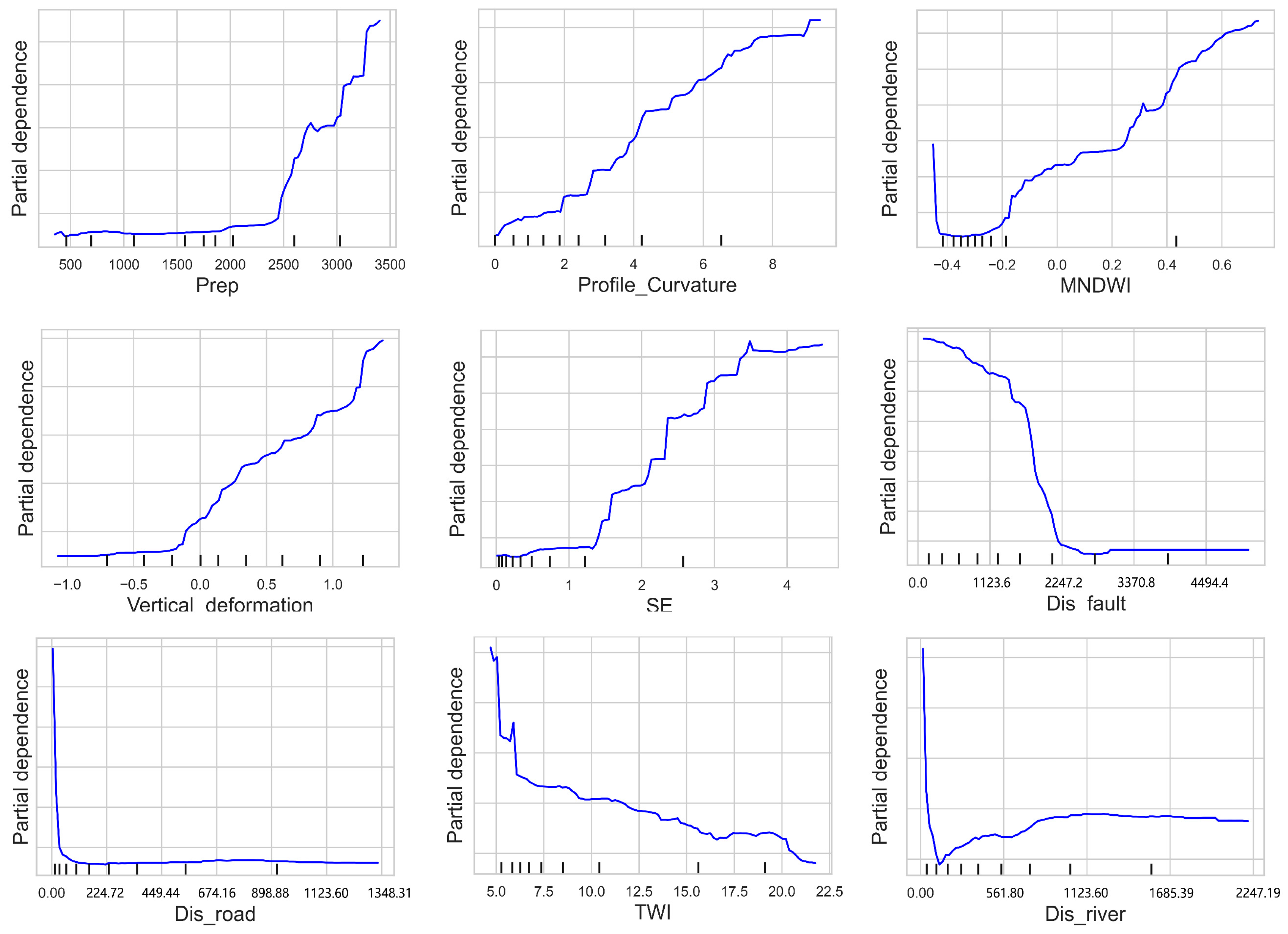
3.4. Nonlinear Relation Analysis

To further explore the relationship between landslide occurrence and various factors, PDPs were generated to study the associations between landslide occurrences and multiple factors. Xinjiang was divided into seven regions based on terrain and landforms
According to Figure 8, six LCFs can be classified into three categories.
First Category: This category includes the MNDWI, Dis_river, and Dis_road. For these LCFs, the probability of landslide occurrence decreases sharply as the factor increases at first, then gradually increases or remains nearly unchanged. Specifically, the MNDWI experiences a sharp decline in landslide probability when below −0.4, remains almost unchanged between −0.4 and −0.2, and then steadily rises when above −0.2. Dis_river decreases sharply when below around 150 m and then gradually increases after surpassing 150 m. Dis_road decreases sharply when below 30 m, and remains nearly constant above 30 m.
Second Category: This category includes SE, Vertical_deformation, Dis_fault, and Prep. These LCFs show clear threshold effects on landslide probability. SE exhibits a near-zero landslide probability when below 1.2, starts to increase between 1.2 and 3.5, and approaches 1 when above 3.5. Vertical_deformation shows a near-zero landslide probability when negative but landslides begin to occur when it turns positive. Dis_fault demonstrates a gradual decrease in landslide probability when below 3000 m, with a near-zero probability beyond 3000 m. Prep starts to induce landslides after exceeding 2500 m.
Third Category: This category includes the TWI and Profile_Curvature. These LCFs do not exhibit clear threshold effects. The TWI shows a negative correlation with landslide probability, whereas Profile_Curvature shows a positive correlation with landslide probability.
Table 6 summarizes the KS statistic and p-values for each variable’s range comparison. The KS statistic measures the maximum difference between cumulative distributions for two groups, in this case, landslide and non-landslide occurrences, and the p-value tests the statistical significance of this difference.
The table reveals that all LCFs show significant KS statistics with corresponding p-values below 0.05, indicating that each of these LCFs plays a statistically significant role in distinguishing landslide from non-landslide areas. Vertical_deformation and Prep show the highest KS statistics (0.401 and 0.449, respectively), suggesting they have the most pronounced difference in distribution between landslide and non-landslide areas.

3.5. Interaction Effect Analysis

In this study, the AUC values for single-factor and two-factor interactions were explored, as shown in Figure 9. The results indicate that most factor combinations exhibit positive interaction effects, suggesting that the combination of two factors yields better classification performance than using each factor individually. These positive interactions typically occur in factor combinations that influence landslide probability in a complementary manner, thus enhancing the model’s predictive power.
However, some factor interactions exhibit negative effects. For instance, interactions between vertical deformation and the TWI, precipitation, and lithology; interactions between slope and precipitation, lithology, and fault distance; interactions between profile curvature and precipitation; interactions between the MNDWI and lithology; and interactions between fault distance and all other factors (except for profile curvature and vertical deformation) all show negative effects. In certain conditions, factors may counteract each other, leading to these negative interactions.
Although lithology has a low AUC value (close to random classification) when considered as a single factor, its importance significantly increases when combined with multiple factors, highlighting its critical role in landslide susceptibility models. This underscores the complexity of geological processes. Lithology alone may not sufficiently explain landslide occurrence, but its interactions with other environmental factors, such as precipitation, slope, and fault distance, can significantly influence landslide risk. Lithology affects the response of soils and rocks under environmental pressures, and its interactions with other factors, such as precipitation and fault distance, can either exacerbate landslide risks, depending on the specific geological context.

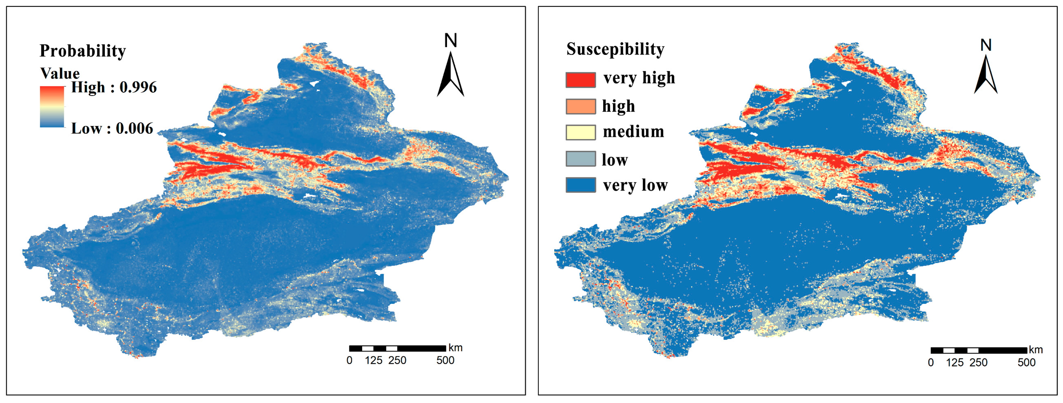
3.6. Spatial Prediction of Landslide Susceptibility

The illustrated results indicate a pronounced spatial differentiation in the landslide susceptibility assessment in Xinjiang (Figure 10), primarily manifested in the following aspects:
The northern regions of Xinjiang, especially near the Tianshan and Altai mountain ranges, exhibit high susceptibility zones, encompassing 3.85% of the total autonomous region’s area. Additionally, a few extremely high susceptibility zones are distributed in the Kunlun mountain range.
High susceptibility zones cover 5.01% of Xinjiang’s total area, sharing similarities in distribution characteristics with extremely high susceptibility zones, predominantly located near mountain ranges.
Moderate susceptibility zones account for 8.15% of Xinjiang’s total area, presenting a basin-shaped morphology.
Low susceptibility zones cover 19.52% of Xinjiang’s total area, whereas extremely low susceptibility zones occupy 63.46% of the area, mainly distributed in the relatively flat areas around the two major basins, the Tarim and Junggar Basins.
The overall trend reveals that the high-incidence areas of landslide geological disasters are mainly concentrated near the Tianshan and Altai mountain ranges, especially in the northern foothills of the Tianshan Mountains and the Ili River Valley, where landslide geological disasters are most severe. The occurrence of landslide geological disasters in Xinjiang exhibits a distinct E-shaped distribution, gradually weakening from west to east.

4. Discussion

4.1. Effectiveness of the GBDT

In the landslide susceptibility assessment using machine learning methods, the reliability of the model is closely related to the training samples, specifically the landslide inventory [56]. However, a landslide catalog cannot encompass all the landslides that occur within a given region. To ensure the temporal and spatial patterns of landslides in the study area are acceptable, we utilized two landslide catalogs from different institutions.
In the landslide susceptibility evaluations, the imbalance between landslide and non-landslide samples presents a series of challenges. When the number of non-landslide samples vastly exceeds the number of landslide samples, the cost of misclassifying landslide samples becomes negligible [45]. Therefore, the selection and quality of non-landslide samples are critical. In such cases, recall is a more appropriate performance metric, focusing on the correct identification of positive samples. In this study, the recall rate for the k-means and BIRCH models was significantly higher than that of the other models, with the k-means model improving recall by 35.4% compared with random selection. This outcome is consistent with the result of another study [47].
Traditional evaluation models are often highly subjective or fail to adequately capture the nonlinear relationships within factors [57]. ML algorithms, on the contrary, excel at modeling these relationships, improving the accuracy of predictions [58,59]. In the landslide susceptibility studies in Xinjiang, many scholars have begun to employ machine learning algorithms for exploration. For example, Yu et al. [60] used the Information-CF model for landslide susceptibility zonation, achieving an AUC of 0.862. Hu et al. [61] employed a coupled model of evidence weights and logistic regression for susceptibility zonation, with an AUC of 0.897. In this study, the GBDT model was selected, achieving an AUC of 0.999, demonstrating its excellent performance in landslide susceptibility assessment [62]. Compared with the studies of Longfei Liang [63] and Chen et al. [64] on landslide susceptibility zonation in Xinjiang, the zonation results are essentially consistent with actual conditions, indicating that landslide disasters are predominantly concentrated in the Tianshan region, especially along the northern slope of the Tianshan Mountains.

4.2. Threshold and Interaction Effects of LCFs

The Xinjiang region, characterized by substantial regional variation and diverse geological conditions, exhibits considerable locality and differences. Landslide susceptibility in different areas is influenced by distinct controlling factors and complex deformation mechanisms, meaning that applicable factors may vary depending on the region.
The study results demonstrate the nonlinear relationship between environmental covariates and landslide susceptibility. Key topographical, geological, and environmental factors were identified as primary drivers of landslide occurrence, with lithology, precipitation, profile curvature, the MNDWI, and vertical deformation emerging as the most influential factors. Notable threshold effects (trigger thresholds) were observed between major LCFs and landslide susceptibility, suggesting that landslides tend to concentrate under specific environmental conditions. The thresholds identified in this study are critical for understanding terrain stability because they mark points where the influence of environmental factors on landslide risk dramatically changes. For instance, precipitation exhibits a strong correlation with landslide occurrence. A threshold of 2500 mm of total precipitation is observed, beyond which the likelihood of landslides increases significantly. This threshold represents a critical level of water infiltration that destabilizes the soil, triggering slope failure. These findings are consistent with previous research on precipitation trigger thresholds, though the focus here is on the specific contextual implications for the study region. The MNDWI, typically used for water body detection, varies significantly due to differences in sensor types and data processing methods [65,66]. The values presented here are for reference. When the MNDWI values are very low, prolonged drought conditions lead to loose soil, making the terrain more susceptible to swelling and sliding when exposed to large amounts of precipitation, which further facilitates the occurrence of landslides and debris flows. At low MNDWI values ranging from −0.4 to −0.2, the slopes remain relatively stable. However, once the MNDWI exceeds −0.2, the increased moisture content initiates landslide activity. This threshold highlights the sensitivity of soil to moisture variations, emphasizing the need for careful monitoring of the MNDWI as a predictor of landslide risk [67]. SE exacerbates landslide risk by weakening soil structure and reducing shear strength. Landslides typically begin when the SE reaches a threshold of 1.2 and peaks at 3.5, indicating the critical role of SE in landslide initiation. Fault zones, where geological structures are fragmented, are more prone to forming weak planes and experiencing seismic events that can trigger landslides. Landslides are more likely to occur near fault zones [68], with no significant landslide occurrences beyond 3000 m from a fault. The distance to fault zones is thus a key factor in landslide prediction, and future studies may benefit from a further exploration of this threshold. The relationship between road proximity and landslide probability is particularly important. Road traffic leads to soil and terrain disturbances, which exert cumulative dynamic stress on the slopes near roads, influencing slope stability [69]. This study identified a clear threshold at 30 m: the probability of landslides decreases sharply when the distance to the road is less than 30 m, but the effect becomes negligible beyond this distance. This indicates that roads within a certain proximity (less than 30 m) significantly disrupt slope stability, and this distance threshold can be used to inform land-use planning and risk mitigation strategies. Finally, vertical deformation provides valuable insight into the likelihood of landslides. Upward deformation, indicating tension in rock layers, increases the potential for erosion and sliding, whereas downward deformation suggests compression and greater rock stability, reducing landslide risk. Landslides are triggered when vertical deformation exceeds 0, underscoring the importance of monitoring this factor in landslide risk assessments [70,71]. These thresholds provide critical insights into terrain stability and have important implications for future studies and landslide mitigation efforts. By incorporating these specific threshold values, future research can refine landslide susceptibility models and improve the accuracy of landslide predictions, aiding in targeted disaster prevention and land-use management strategies.
This study reveals the interactions between various environmental factors and their significance in landslide susceptibility prediction. The occurrence of landslides is not only influenced by individual factors but by the complex interactions among multiple factors. Positive interactions indicate that the synergistic effects between factors can enhance the accuracy of the model. Specifically, the interaction between lithology and precipitation can significantly alter landslide risk assessments. Certain types of lithology, in combination with high precipitation, may cause soil expansion or instability, thereby increasing the risk of landslides. Under certain lithological conditions, excessive precipitation leads to changes in the soil’s physical and chemical properties, increasing soil expansion or instability, which in turn significantly elevates the probability of landslides [72]. On the contrary, negative interaction effects suggest the presence of antagonistic relationships between factors. For example, the negative interaction between vertical deformation and the TWI implies that the vertical deformation may attenuate the influence of the TWI, thereby reducing the probability of landslides. When vertical deformation is below 0, compression enhances rock stability, which strengthens the soil structure and counteracts the potential risk of landslides in wet conditions [73]. The presence of negative interaction effects suggests that the relationships between factors are more complex than the influence of individual factors alone. Therefore, future research should further explore these interactions and validate their contributions to landslide prediction models.
The study of these interactions is not only of theoretical importance but holds significant practical value. Understanding the interactions between factors provides a critical basis for accurate landslide risk prediction and the development of effective mitigation strategies. By identifying key factors and their interactions, future landslide risk assessment models can precisely identify high-risk areas. For example, for specific interactions between lithology and precipitation, targeted disaster prevention strategies can be designed in high-precipitation areas, such as enhancing soil stability or improving soil and water conservation measures. By tailoring early warning systems to different types of factor interactions, landslide risk prediction models can be customized, providing accurate decision-making support for local governments and relevant authorities.
The precise selection of the number and type of evaluation factors forms the foundation of landslide susceptibility assessments. The choice of factor types is typically based on field surveys and data analysis, but no unified standard exists for determining the number of factors. Using too many factors may lead to increased data volume and longer evaluation times, whereas too few factors may fail to reveal the underlying relationships between landslide triggers. Therefore, selecting appropriate evaluation factors during the preliminary investigation and analysis of landslide hazards in the study area is crucial. Performing such an evaluation helps to improve the accuracy of the susceptibility evaluation results and provides effective disaster prevention and reduction strategies for regions affected by landslides.

4.3. Limitations

Previous studies have shown that factors such as stratigraphy, soil texture, bulk density, and groundwater depth can reflect the inherent characteristics of geology or soil, and integrating these factors can better explain landslide susceptibility [56,74]. However, because of data limitations, this study was unable to incorporate these key factors into the model. This limitation may lead to bias in assessing landslide susceptibility, particularly in areas significantly influenced by these factors. The missing data could obscure important geological features affecting the accuracy of landslide risk assessments.
Moreover, Xinjiang is a large-scale region, and some of the data used in this study (such as vertical deformation, landforms, and precipitation) have a relatively high resolution, which limits the applicability of the model in other areas. High-resolution data can provide more detailed geological and environmental features, and using lower-resolution data could distort the results of a landslide susceptibility analysis, especially in areas with dramatic topographic variations.
While the GBDT captures nonlinear patterns effectively, its interpretability relies on post hoc tools, like partial dependence plots (PDPs), which face three key constraints. First, PDPs assume feature independence when estimating marginal effects, oversimplifying collinear relationships (e.g., rainfall–soil permeability interactions) common in geospatial data. This can lead to an erroneous attribution of synergistic effects to individual factors [75]. Second, the GBDT’s sensitivity to hyperparameters (e.g., tree depth) amplifies the PDP’s instability, as minor parameter adjustments may drastically alter interpretation outcomes [76].
While stratigraphic, soil texture, and hydrological parameters (e.g., bulk density, groundwater depth) could theoretically complement rainfall dynamics by revealing inherent geological vulnerabilities [77], their exclusion due to data gaps creates compounded biases, particularly in regions where soil–water interactions dominate failure mechanisms. This data scarcity mirrors the temporal resolution challenges of rainfall parameters, as both static geological characteristics and dynamic hydrological processes require high-resolution spatiotemporal monitoring to capture their synergistic effects [77,78].

5. Conclusions

This study employed the GBDT model for LSM, identification of key controlling factors, and investigation of threshold and interaction effects. The results showed that the GBDT model achieved an AUC value of 0.937, 11.3% higher than the second-best SVM model (0.842). After incorporating clustering algorithms to select non-landslide samples, the recall value remained high at 0.963, representing a 21.4% improvement over random sampling (0.711), demonstrating robust performance. The GBDT model revealed that areas with extremely high and high landslide susceptibility accounted for 8.86% of Xinjiang, primarily concentrated around the Tianshan and Altai mountain ranges with an E-shaped distribution. Landslide occurrence was mainly influenced by lithology, precipitation, profile curvature, the MNDWI, and vertical deformation, which together explained 92.86% of landslides. Importantly, the relationships between these factors and landslide susceptibility exhibited threshold effects. The probability of landslides increased significantly when precipitation exceeded 2500 mm. At MNDWI values greater than −0.2, landslides began to occur as moisture content increased. SE values above 1.2 triggered landslides, reaching their peak at 3.5. When the distance to roads (Dis_road) was less than 30 m, landslide probability sharply decreased, with landslides virtually ceasing beyond 30 m. Vertical deformation initiated landslides when it exceeded 0. Additionally, the influence of bivariate interaction effects was confirmed. Although a small proportion of interactions were negative, the majority of factor interactions were positive, where the combination of two factors produced better classification results than individual factors. These findings suggest that the influence of these factors on landslide occurrence is complex and interactive, rather than a simple additive effect.

Author Contributions

Conceptualization, X.F. and Z.W. (Zihao Wu); Methodology, X.F.; Software, X.F. and Z.W. (Zihao Wu); Validation, J.B. and S.L.; Formal analysis, X.F. and Z.W. (Zhaoqi Wu); Investigation, X.F.; Resources, Z.W. (Zhaoqi Wu), J.B. and S.L.; Data curation, Z.W. (Zhaoqi Wu), J.B. and S.L.; Writing—original draft, X.F. and Z.W. (Zhaoqi Wu); Writing—review & editing, Z.W. (Zihao Wu) and Q.Y.; Visualization, X.F.; Supervision, Z.W. (Zihao Wu); Project administration, Z.W. (Zihao Wu) and Q.Y. All authors have read and agreed to the published version of the manuscript.

Funding

This paper was supported by the Third Comprehensive Scientific Expedition to Xinjiang in China-Geological Hazards and Ecological Environment Investigation of National Major Energy Channel on the North Slope of Tianshan Mountains (Grant Number 2022xjkk1004) and the National Natural Science Foundation of China (Grant Number 42201447), and did not receive other external funding.

Data Availability Statement

Data are contained within the article. Further inquiries can be directed to the corresponding author.

Acknowledgments

The authors acknowledge data support from “National Earth System Science Data Center, National Science and Technology Infrastructure of China (http://www.geodata.cn, accessed on 25 February 2025)” and “National Tibetan Plateau/Third Pole Environment Data Center (http://data.tpdc.ac.cn, accessed on 25 February 2025)”.

Conflicts of Interest

Author Junping Bai was employed by the company Xinjiang Power Transmission and Transformation Co., Ltd. Author Shixiang Liu was employed by the company Zhongdihuaan Science and Technology Co., Ltd. The remaining authors declare that the research was conducted in the absence of any commercial or financial relationships that could be construed as a potential conflict of interest.

References

  1. Boubazine, L.; Boumezbeur, A.; Hadji, R.; Kessasra, F. Slope failure characterization: A joint multi-geophysical and geotechnical analysis, case study of Babor Mountains range, NE Algeria. Min. Miner. Depos. 2022, 16, 65–70. [Google Scholar] [CrossRef]
  2. Feizizadeh, B.; Roodposhti, M.S.; Jankowski, P.; Blaschke, T. A GIS-based extended fuzzy multi-criteria evaluation for landslide susceptibility mapping. Comput. Geosci. 2014, 73, 208–221. [Google Scholar] [CrossRef]
  3. Froude, M.J.; Petley, D.N. Global fatal landslide occurrence from 2004 to 2016. Nat. Hazards Earth Syst. Sci. 2018, 18, 2161–2181. [Google Scholar] [CrossRef]
  4. Li, W.; Zhu, J.; Fu, L.; Zhu, Q.; Guo, Y.; Gong, Y. Arapid 3D reproduction system ofdam-break floods constrained by post-disaster information. Environ. Modell. Softw. 2021, 139, 104994. [Google Scholar] [CrossRef]
  5. Li, W.; Zhu, J.; Fu, L.; Zhu, Q.; Xie, Y.; Hu, Y. An augmented representation method of debris flow scenes to improve public perception. Int. J. Geogr. Inf. Sci. 2021, 35, 1521–1544. [Google Scholar] [CrossRef]
  6. Wang, Z.; Xu, S.; Liu, J.; Wang, Y.; Ma, X.; Jiang, T.; He, X.; Han, Z. A Combination of Deep Autoencoder and Multi-Scale Residual Network for Landslide Susceptibility Evaluation. Remote Sens. 2023, 15, 653. [Google Scholar] [CrossRef]
  7. Shichuan, L.; Hua, Q.; Dong, L.; Qiang, H. Distribution characteristics and main controlling factors of geohazards in Ili Valley. Arid Land Geogr. 2023, 46, 880–888. [Google Scholar]
  8. Borrelli, L.; Ciurleo, M.; Gulla, G. Shallow landslide susceptibility assessment in granitic rocks using GIS-based statistical methods: The contribution of the weathering grade map. Landslides 2018, 15, 1127–1142. [Google Scholar] [CrossRef]
  9. Ciampalini, A.; Raspini, F.; Lagomarsino, D.; Catani, F.; Casagli, N. Landslide susceptibility map refinement using PSInSAR data. Remote Sens. Environ. 2016, 184, 302–315. [Google Scholar] [CrossRef]
  10. Wu, W.; Zhang, Q.; Singh, V.P.; Wang, G.; Zhao, J.; Shen, Z.; Sun, S. A Data-Driven Model on Google Earth Engine for Landslide Susceptibility Assessment in the Hengduan Mountains, the Qinghai-Tibetan Plateau. Remote Sens. 2022, 14, 4662. [Google Scholar] [CrossRef]
  11. Bhandary, N.P.; Dahal, R.K.; Timilsina, M.; Yatabe, R. Rainfall event-based landslide susceptibility zonation mapping. Nat. Hazards 2013, 69, 365–388. [Google Scholar] [CrossRef]
  12. Hong, H.; Naghibi, S.A.; Pourghasemi, H.R.; Pradhan, B. GIS-based landslide spatial modeling in Ganzhou City, China. Arab. J. Geosci. 2016, 9, 112. [Google Scholar] [CrossRef]
  13. Regmi, N.R.; Giardino, J.R.; Vitek, J.D. Assessing susceptibility to landslides: Using models to understand observed changes in slopes. Geomorphology 2010, 122, 25–38. [Google Scholar] [CrossRef]
  14. Van Westen, C.J.; Castellanos, E.; Kuriakose, S.L. Spatial data for landslide susceptibility, hazard, and vulnerability assessment: An overview. Eng. Geol. 2008, 102, 112–131. [Google Scholar] [CrossRef]
  15. Akgun, A.; Kıncal, C.; Pradhan, B. Application of remote sensing data and GIS for landslide risk assessment as an environmental threat to Izmir city (west Turkey). Environ. Monit. Assess. 2012, 184, 5453–5470. [Google Scholar] [CrossRef]
  16. Huang, J.; Zeng, X.; Ding, L.; Yin, Y.; Li, Y. Landslide Susceptibility Evaluation Using Different Slope Units Based on BP Neural Network. Comput. Intell. Neurosci. 2022, 2022, 9923775. [Google Scholar] [CrossRef]
  17. Chen, W.; Sun, Z.; Han, J. Landslide Susceptibility Modeling Using Integrated Ensemble Weights of Evidence with Logistic Regression and Random Forest Models. Appl. Sci. 2019, 9, 171. [Google Scholar] [CrossRef]
  18. Hong, H.; Pourghasemi, H.R.; Pourtaghi, Z.S. Landslide susceptibility assessment in Lianhua County (China): A comparison between a random forest data mining technique and bivariate and multivariate statistical models. Geomorphology 2016, 259, 105–118. [Google Scholar] [CrossRef]
  19. Trigila, A.; Iadanza, C.; Esposito, C.; Scarascia-Mugnozza, G. Comparison of Logistic Regression and Random Forests techniques for shallow landslide susceptibility assessment in Giampilieri (NE Sicily, Italy). Geomorphology 2015, 249, 119–136. [Google Scholar] [CrossRef]
  20. Zhou, C.; Yin, K.; Cao, Y.; Ahmed, B.; Li, Y.; Catani, F.; Pourghasemi, H.R. Landslide susceptibility modeling applying machine learning methods: A case study from Longju in the Three Gorges Reservoir area, China. Comput. Geosci. 2018, 112, 23–37. [Google Scholar] [CrossRef]
  21. Wang, Y.; Fang, Z.; Niu, R.; Peng, L. Landslide susceptibility analysis based on deep learning. J. Geo-Inf. Sci. 2021, 23, 2244–2260. [Google Scholar]
  22. Wu, R.; Hu, X.; Mei, H.; He, J.; Yang, J. Spatial Susceptibility Assessment of Landslides Basedon Random Forest: A Case Study from Hubei Sectionin the Three Gorges Reservoir Area. Earth Sci. 2021, 46, 321–330. [Google Scholar]
  23. Abbas, F.; Zhang, F.; Abbas, F.; Ismail, M.; Iqbal, J.; Hussain, D.; Khan, G.; Alrefaei, A.F.; Albeshr, M.F. Landslide Susceptibility Mapping: Analysis of Different Feature Selection Techniques with Artificial Neural Network Tuned by Bayesian and Metaheuristic Algorithms. Remote Sens. 2023, 15, 4330. [Google Scholar] [CrossRef]
  24. Zhao, L.; Wu, X.; Niu, R.; Wang, Y.; Zhang, K. Using the rotation and random forest models of ensemble learning to predict landslide susceptibility. Geomat. Nat. Hazards Risk 2020, 11, 1542–1564. [Google Scholar] [CrossRef]
  25. Demczuk, P.; Zydroń, T.; Siłuch, M. Rainfall thresholds for the occurrence of shallow landslides determined for slopes in the Nowy Wiśnicz Foothills (Polish Flysch Carpathians). Geol. Q. 2019, 63, 822–838. [Google Scholar] [CrossRef]
  26. Huang, F.; Xiong, H.; Yao, C.; Catani, F.; Zhou, C.; Huang, J. Uncertainties of landslide susceptibility prediction considering different landslide types. J. Rock Mech. Geotech. Eng. 2023, 15, 2954–2972. [Google Scholar] [CrossRef]
  27. Shu, H.; He, J.; Zhang, F.; Zhang, M.; Ma, J.; Chen, Y.; Yang, S. Construction of landslide warning by combining rainfall threshold and landslide susceptibility in the gully region of the Loess Plateau: A case of Lanzhou City, China. J. Hydrol. 2024, 645, 132148. [Google Scholar] [CrossRef]
  28. Rohan, T.; Shelef, E.; Bain, D.; Ramsey, M.S.; Werne, J.; Iannacchione, A.Z. Enhancing Landslide Susceptibility Analysis through Citizen Science, Geospatial Analysis, and Precipitation Thresholds in Urbanizing Environments. Doctoral Dissertation, University of Pittsburgh, Pittsburgh, PA, USA, 2023. [Google Scholar]
  29. Avci, P.; Ercanoglu, M. Utilization of streamflow rates for determination of precipitation thresholds for landslides in a data-scarce region (Eastern Bartın, NW Türkiye). Environ. Earth Sci. 2024, 83, 192. [Google Scholar] [CrossRef]
  30. Li, Y.; Ming, D.; Zhang, L.; Niu, Y.; Chen, Y. Seismic Landslide Susceptibility Assessment Using Newmark Displacement Based on a Dual-Channel Convolutional Neural Network. Remote Sens. 2024, 16, 566. [Google Scholar] [CrossRef]
  31. Jinrui, Z.; Yang, W.; Xiao, F.; Yuanyao, L.; Bijing, J.; Chao, Z.; Xin, Z.; Yang, D. Analysis of spatial-temporal variations in landslide susceptibility assessment considering surface deformation and land use dynamics. Bull. Geol. Sci. Technol. 2024, 43, 184–195. [Google Scholar]
  32. Abbaszadeh Shahri, A.; Spross, J.; Johansson, F.; Larsson, S. Landslide susceptibility hazard map in southwest Sweden using artificial neural network. CATENA 2019, 183, 104225. [Google Scholar] [CrossRef]
  33. Wu, Z.; Chen, Y.; Zhu, Y.; Feng, X.; Ou, J.; Li, G.; Tong, Z.; Yan, Q. Mapping Soil Organic Carbon in Floodplain Farmland: Implications of Effective Range of Environmental Variables. Land 2023, 12, 1198. [Google Scholar] [CrossRef]
  34. Zhang, Z.; Zhang, T.; Yu, X.; Lv, Q.; Lai, R.; Jia, J.; Liu, X. Zonation of Disaster Environments of Collapse, Landslide and Debris Flow Geologic Hazards and Their Formation Mechanisms in Xinjiang. J. Eng. Geol. 2023, 31, 1129–1144. [Google Scholar] [CrossRef]
  35. Jiang, Y.; Wang, W.; Zou, L.; Cao, Y. Regional landslide susceptibility assessment based on improved semi-supervised clustering and deep learning. Acta Geotech. 2024, 19, 509–529. [Google Scholar] [CrossRef]
  36. Guo, Z.; Shi, Y.; Huang, F.; Fan, X.; Huang, J. Landslide susceptibility zonation method based on C5.0 decision tree and K-means cluster algorithms to improve the efficiency of risk management. Geosci. Front. 2021, 12, 101249. [Google Scholar] [CrossRef]
  37. Wu, Z.; Zhao, S. A Study of Enhanced Index based Built-up Index Based on Landsat TM Imagery. Remote Sens. Land Resour. 2012, 24, 50–55. [Google Scholar] [CrossRef]
  38. Xu, H. A Study on Information Extraction of Water Body with the Modified Norm a lized Difference Water Index (MNDWI). J. Remote Sens. 2005, 5, 589–595. [Google Scholar] [CrossRef]
  39. Li, J.; He, H.; Zeng, Q.; Chen, L.; Sun, R. A Chinese soil conservation dataset preventing soil water erosion from 1992 to 2019. Sci. Data 2023, 10, 319. [Google Scholar] [CrossRef]
  40. Zhou, P.; Deng, H.; Jiang, W.; Xue, D.; Wu, X.; Zhuo, W. Landslide Susceptibility Evaluation Based on Information Value Modeland Machine Learning Method: A Case Study of Lixian County, Sichuan Province. Sci. Geogr. Sin. 2022, 42, 1665–1675. [Google Scholar] [CrossRef]
  41. Chen, W.; Xie, X.; Wang, J.; Pradhan, B.; Hong, H.; Bui, D.T.; Duan, Z.; Ma, J. A comparative study of logistic model tree, random forest, and classification and regression tree models for spatial prediction of landslide susceptibility. CATENA 2017, 151, 147–160. [Google Scholar] [CrossRef]
  42. Tien Bui, D.; Tuan, T.A.; Hoang, N.-D.; Thanh, N.Q.; Nguyen, D.B.; Van Liem, N.; Pradhan, B. Spatial prediction of rainfall-induced landslides for the Lao Cai area (Vietnam) using a hybrid intelligent approach of least squares support vector machines inference model and artificial bee colony optimization. Landslides 2017, 14, 447–458. [Google Scholar] [CrossRef]
  43. Malmgren-Hansen, D.; Sohnesen, T.; Fisker, P.; Baez, J. Sentinel-1 Change Detection Analysis for Cyclone Damage Assessment in Urban Environments. Remote Sens. 2020, 12, 2409. [Google Scholar] [CrossRef]
  44. Iotti, M.; Bonazzi, G. Tomato Processing Firms’ Management: A Comparative Application of Economic And Financial Analyses. Am. J. Appl. Sci. 2014, 11, 1135–1151. [Google Scholar] [CrossRef]
  45. Mwakapesa, D.S.; Lan, X.; Mao, Y. Landslide susceptibility assessment using deep learning considering unbalanced samples distribution. Heliyon 2024, 10, e30107. [Google Scholar] [CrossRef]
  46. Huang, F.; Yin, K.; Huang, J.; Gui, L.; Wang, P. Landslide susceptibility mapping based on self-organizing-map network and extreme learning machine. Eng. Geol. 2017, 223, 11–22. [Google Scholar] [CrossRef]
  47. Liu, C. Optimization of negative sample selection for landslide susceptibility mapping based on machine learning using K-means-KNN algorithm. Earth Sci. Inform. 2023, 16, 4131–4152. [Google Scholar] [CrossRef]
  48. Czarnecki, W.M.; Podlewska, S.; Bojarski, A.J. Robust optimization of SVM hyperparameters in the classification of bioactive compounds. J. Cheminform. 2015, 7, 38. [Google Scholar] [CrossRef]
  49. Li, A.; La, J.; May, S.B.; Guffey, D.; da Costa, W.L.; Amos, C.I.; Bandyo, R.; Milner, E.M.; Kurian, K.M.; Chen, D.C.R.; et al. Derivation and Validation of a Clinical Risk Assessment Model for Cancer-Associated Thrombosis in Two Unique US Health Care Systems. J. Clin. Oncol. 2023, 41, 2926–2938. [Google Scholar] [CrossRef]
  50. Friedman, J.H. Greedy function approximation: A gradient boosting machine. Ann. Stat. 2002, 29, 1189–1232. [Google Scholar] [CrossRef]
  51. Luque, A.; Carrasco, A.; Martín, A.; De Las Heras, A. The impact of class imbalance in classification performance metrics based on the binary confusion matrix. Pattern Recognit. 2019, 91, 216–231. [Google Scholar] [CrossRef]
  52. Gneiting, T.; Vogel, P. Receiver operating characteristic (ROC) curves: Equivalences, beta model, and minimum distance estimation. Mach. Learn. 2021, 111, 2147–2159. [Google Scholar] [CrossRef]
  53. Gorsevski, P.V.; Gessler, P.E.; Foltz, R.B.; Elliot, W.J. Spatial Prediction of Landslide Hazard Using Logistic Regression and ROC Analysis. Trans. GIS 2006, 10, 395–415. [Google Scholar] [CrossRef]
  54. Riegel, R.P.; Alves, D.D.; Schmidt, B.C.; De Oliveira, G.G.; Haetinger, C.; Osório, D.M.M.; Rodrigues, M.A.S.; De Quevedo, D.M. Assessment of susceptibility to landslides through geographic information systems and the logistic regression model. Nat. Hazards 2020, 103, 497–511. [Google Scholar] [CrossRef]
  55. Changrun, W.; Yuanmei, J.; Jinliang, W.; Hanhua, X.; Hua, Z.; Qiue, X. Frequency ratio and logistic regression models based coupling analysis for susceptibility of landslide in Shuangbai County. J. Nat. Disasters 2021, 30, 213–224. [Google Scholar]
  56. Reichenbach, P.; Rossi, M.; Malamud, B.D.; Mihir, M.; Guzzetti, F. A review of statistically-based landslide susceptibility models. Earth-Sci. Rev. 2018, 180, 60–91. [Google Scholar] [CrossRef]
  57. Dickson, M.E.; Perry, G.L.W. Identifying the controls on coastal cliff landslides using machine-learning approaches. Environ. Model. Softw. 2016, 76, 117–127. [Google Scholar] [CrossRef]
  58. Fang, R.; Liu, Y.; Huang, Z. A review of the methods of regional landslide hazard assessment based on machine learning. Chin. J. Geol. Hazard Control 2021, 32, 1–8. [Google Scholar] [CrossRef]
  59. Wang, G.; Guo, N.; Deng, B.; Tian, Y.; Ye, Z.; Xu, Z.; Xu, F.; Gao, Y. Analysis of Landslide Susceptibility and Accuracy in Different Combination Models. Northwestern Geol. 2021, 54, 259–272. [Google Scholar] [CrossRef]
  60. Yu, X.; Zhang, Z.; Shi, G.; Li, C.; Liu, Y.; Zhu, J.; Chen, W. Evaluation of Geological Hazard Susceptibility Inemincounty, Xinjiang Based on Deterministic Coefficient and Information Coupling Model. J. Eng. Geol. 2023, 31, 1333–1349. [Google Scholar] [CrossRef]
  61. Hu, Y.; Zizhao, Z.; Lin, S. Evaluation of Landslide Susceptibility in Ili Valley, XinJiang Based on the Coupling of Woe Model and Logistic Regression. J. Eng. Geol. 2023, 31, 1350–1363. [Google Scholar] [CrossRef]
  62. Li, M.; Jiang, W.; Dong, J.; Jin, S.; Zhang, C.; Niu, R. Evaluation of landslide hazards susceptibility based on machine learning:Taking the Three Gorges Reservoir Area as an Example. South China Geol. 2023, 39, 413–427. [Google Scholar] [CrossRef]
  63. Liang, L. Application of Small-Sample Machine Learning Method Inevaluation of Landslide Disaster Susceptibility in Xinjiang. J. Eng. Geol. 2023, 31, 1394–1406. [Google Scholar] [CrossRef]
  64. Chen, K.; Chen, L.; Zhang, Z.; Chang, Y. Susceptibility and risk assessment of geological disasters in Xinjiang based on empirical investigation. J. Eng. Geol. 2023, 31, 1156–1166. [Google Scholar] [CrossRef]
  65. Nian, T.-K.; Feng, Z.-K.; Yu, P.-C.; Wu, H.-J. Strength behavior of slip-zone soils of landslide subject to the change of water content. Nat. Hazards 2013, 68, 711–721. [Google Scholar] [CrossRef]
  66. Cui, P.; Guo, J. Evolution Models, Risk Prevention and Control Countermeasures of the Valley Disaster Chain. Adv. Eng. Sci. 2021, 53, 5–18. [Google Scholar] [CrossRef]
  67. Wen, H.; Ni, S.M.; Wang, Y.T.; Wang, J.G.; Cai, C.F. A Study on Silty Soil Shear Strength and Its Influencing Factors in Different Vegetation Types in Benggang Erosion Area of Southern Jiangxi. Acta Pedofil. Sin. 2022, 59, 1517–1526. [Google Scholar] [CrossRef]
  68. Li, Y.; Zhang, H.; Huang, L.; Li, H.; Wu, X. The formation mechanism of landslides in typical fault zones and protective countermeasures: A case study of the Nanpeng River fault zone. Front. Earth Sci. 2023, 10, 1092662. [Google Scholar] [CrossRef]
  69. Sadeghi, S.; Solgi, A.; Tsioras, P.A. Effects of traffic intensity and travel speed on forest soil disturbance at different soil moisture conditions. Int. J. For. Eng. 2022, 33, 146–154. [Google Scholar] [CrossRef]
  70. Ye, K.; Wang, Z.; Wang, T.; Luo, Y.; Chen, Y.; Zhang, J.; Cai, J. Deformation Monitoring and Analysis of Baige Landslide (China) Based on the Fusion Monitoring of Multi-Orbit Time-Series InSAR Technology. Sensors 2024, 24, 6760. [Google Scholar] [CrossRef]
  71. Deng, L.; Yuan, H.; Zhang, M.; Chen, J. Research progress on landslide deformation monitoring and early warning technology. J. Tsinghua Univ. (Sci. Technol.) 2023, 63, 849–864. [Google Scholar] [CrossRef]
  72. Ya, Z.; Wei, H.; Meng, L. Analysis on the Distribution and Drivers of Flash Floods in Yunnan Province. J. Catastrophaol. 2018, 33, 96–100. [Google Scholar]
  73. Wang, J. Prediction and Risk Analysis of Reservoir Bank Landslide Under the Combined Action of Rainfall and Reservoir Water Level: A Case Study of Xinpu Landslide in Three Gorges Reservoir Area. Master’s Thesis, Changan Unicersity, Xi’an, China, 2021. [Google Scholar]
  74. Merghadi, A.; Yunus, A.P.; Dou, J.; Whiteley, J.; ThaiPham, B.; Bui, D.T.; Avtar, R.; Abderrahmane, B. Machine learning methods for landslide susceptibility studies: A comparative overview of algorithm performance. Earth-Sci. Rev. 2020, 207, 103225. [Google Scholar] [CrossRef]
  75. Goetz, J.N.; Brenning, A.; Petschko, H.; Leopold, P. Evaluating machine learning and statistical prediction techniques for landslide susceptibility modeling. Comput. Geosci. 2015, 81, 1–11. [Google Scholar] [CrossRef]
  76. Probst, P.; Boulesteix, A.-L.; Bischl, B. Tunability: Importance of hyperparameters of machine learning algorithms. J. Mach. Learn. Res. 2019, 20, 1934–1965. [Google Scholar]
  77. Gyamfi, C.; Ndambuki, J.; Salim, W. A Historical Analysis of Rainfall Trend in the Olifants Basin in South Africa. Earth Sci. Res. 2016, 5, 129. [Google Scholar] [CrossRef]
  78. Leyva, S.; Cruz-Pérez, N.; Rodríguez-Martín, J.; Miklin, L.; Santamarta, J.C. Rockfall and Rainfall Correlation in the Anaga Nature Reserve in Tenerife (Canary Islands, Spain). Rock Mech. Rock Eng. 2022, 55, 2173–2181. [Google Scholar] [CrossRef]
Figure 1. Overview of the study area.
Land 14 00555 g001
Figure 2. (al) Spatial distribution of certain LCFs.
Land 14 00555 g002
Figure 3. Flowchart of the LSM.
Land 14 00555 g003
Figure 4. Spearman’s correlation coefficient matrix. In the Figure, “Depth_T_B” represents Depth to Bedrock, “Vertical_D” represents Vertical deformation, and “Profile_C” represents Profile Curvature.
Land 14 00555 g004
Figure 5. The ROC curve of the model.
Land 14 00555 g005
Figure 6. Model accuracy line graph of different clustering methods.
Land 14 00555 g006
Figure 7. Relative importance chart.
Land 14 00555 g007
Figure 8. Partial dependence plot.
Land 14 00555 g008
Figure 9. Interaction effect diagram.
Land 14 00555 g009
Figure 10. Landslide susceptibility assessment.
Land 14 00555 g010
Table 1. Index system and data source.
ConditionTypeLCFsData Sources and Links
Internal
conditions
TopographyElevationGeospatial Data Cloud
(https://www.gscloud.cn/, accessed on 25 February 2025)
Slope, Profile Curvature, TWI, TRI, AspectDigital Elevation Model
LandformsChinese Academy Of Sciences
Resource And Environment Science And Data Center
(https://www.resdc.cn/, accessed on 25 February 2025)
GeologyDepth to bedrockISRIC
World Soil Information
(https://www.isric.org/, accessed on 25 February 2025)
Dis_faultGeoscientific Data Discovery Publishing System
(http://dcc.ngac.org.cn/, accessed on 25 February 2025)
LithologyUSGS
Geosciences and Environmental Change Science Center
(https://www.usgs.gov/, accessed on 25 February 2025)
External
conditions
Land coverLandcover
NDBBI, MNDWI, NDVILandsat8
Remote sensing imagery
HydrologyPrepPANGAEA Data Publisher
(https://doi.pangaea.de/, accessed on 25 February 2025)
Dis_riverOpenStreetMap
(https://www.openstreetmap.org/, accessed on 25 February 2025)
Human activitiesDis_road
Dis_mineGlobal Disaster Data Platform
(https://www.gddat.cn/, accessed on 25 February 2025)
Other factorsVertical deformationNational Earth System Science Data Center
(http://www.geodata.cn, accessed on 25 February 2025)
SEZenodo
(https://zenodo.org/, accessed on 25 February 2025)
Table 2. Confusion matrix.
Actual Positive ExampleActual Negative Examples
Predict positive examplesTPFP
Predict negative examplesFNTN
Table 3. Model accuracy across different models.
ModelAUCRecallKS StatisticLogLossPRAUC
LR0.8020.2420.6260.3940.724
SVM0.8420.1580.7560.3850.848
DNN0.8070.1670.7461.2430.847
GBDT0.9370.6240.7930.2350.903
Table 4. Model accuracy for different clustering methods.
Cluster Typek-MeansHCBIRCHMean_ShiftCG
AUC0.9990.9850.9990.9820.981
AUC_STD0.0000.0030.0000.0020.003
Recall0.9630.7670.9500.7230.711
Recall_STD0.0080.0130.0100.0200.010
KS Statistic0.9760.8960.9650.8630.848
KS Statistic_STD0.0060.0150.0050.0070.014
LogLoss0.0310.1120.0370.1390.143
LogLoss_STD0.0020.0050.0020.0030.003
PRAUC0.9970.9500.9940.9290.921
PRAUC_STD0.0020.0070.0010.0060.011
Table 5. Reasonableness test results of landslide hazard prone zoning based on the GBDT model.
Susceptibility LevelSaiGeiRei = Gei/Sai
Very low susceptibility I63.46%0.92%0.01
Low susceptibility II19.52%3.63%0.19
Medium susceptibility III8.15%4.92%0.60
High susceptibility IV5.01%8.85%1.77
Very high susceptibility V3.85%81.68%21.22
Table 6. KS test of the threshold.
VariableRange1Range2KS-Statisticp-Value
MNDWI<−0.4>−0.40.1410.000
MNDWI<−0.2>−0.20.2820.000
Dis_river<150>1500.0560.018
Dis_road<30>300.0720.008
SE<1.2>1.20.0610.000
SE<3.5>3.50.0900.000
Vertical_deformation<0>00.4010.000
Dis_fault<3000>30000.3260.000
Prep<2500>25000.4490.000
Disclaimer/Publisher’s Note: The statements, opinions and data contained in all publications are solely those of the individual author(s) and contributor(s) and not of MDPI and/or the editor(s). MDPI and/or the editor(s) disclaim responsibility for any injury to people or property resulting from any ideas, methods, instructions or products referred to in the content.

