Article

Unequal Impact of Road Expansion on Regional Ecological Quality

College of Transportation and Civil Engineering, Fujian Agriculture and Forestry University, Fuzhou 350002, China
*
Author to whom correspondence should be addressed.
Land 2025, 14(3), 523; https://doi.org/10.3390/land14030523
Submission received: 2 February 2025 / Revised: 27 February 2025 / Accepted: 28 February 2025 / Published: 3 March 2025

Abstract

:
The expansion of road networks profoundly affects ecological systems by intensifying habitat fragmentation, altering hydrological processes, and exacerbating pollution. However, our understanding of the multi-scale spatiotemporal coupling between road networks and ecological quality remains limited. Thus, taking Fuzhou City in Southeastern China as a case study (~12,000 km2), we apply bivariate spatial autocorrelation, geographical detectors (GDs), and multi-scale geographically weighted regression (MGWR) to explore the multi-scale interactions between road networks and ecological quality. Results reveal the following: (1) From 2016 to 2021, kernel density estimation (KDE) analysis of the road network indicates coordinated growth in both urban and rural areas, with an increase of 0.759 km/km2. Analysis based on the remote sensing-based ecological index (RSEI) shows a decrease from 2000 to 2016, and then an increase from 2016 to 2021, with a trend of increasing gradually from urban center to rural area. (2) Predominant tradeoff relationships exist between KDE and RSEI in 2016 and 2021, while notable synergistic relationships emerge between ΔKDE and ΔRSEI. (3) Multi-scale GD analysis identifies ΔKDE as a principal factor influencing ΔRSEI, and the MGWR reveals their significant synergistic associations at an optimal scale of 3000 m. These findings highlight the unequal impact of road network expansion on ecological quality, underscoring the pivotal role of road density changes in its spatiotemporal dynamics. They offer essential insights for sustainable transport and ecological planning.

1. Introduction

The rapid expansion of the global road network is driven by various factors, including regional trade, transportation, and tourism demands [1]. It is projected that by 2050, there will be 25 million kilometers of newly constructed roads worldwide, enough to encircle the Earth’s equator more than 600 times, with nine-tenths of these roads located in developing countries [2,3]. As critical infrastructure for human activities, the road network connects cities and rural areas, facilitating human interaction and resource flow [4]. However, while road construction can promote social and economic development, it also opens Pandora’s box of environmental issues [5]. The direct and indirect impacts of road construction and transportation on the ecological environment have garnered widespread attention. Road construction affects ecological quality, biodiversity, and ecosystem stability [6,7,8]. Furthermore, road traffic influences environmental metrics such as land use, air quality, and noise, particularly in urban regions [9,10,11,12].
In China, roads form the backbone of transportation, supporting 63.5% of passenger transport and 73.3% of freight traffic. By the end of 2022, China’s total road mileage reached 5.35 million kilometers, including 177,000 km of expressways and 2.53 million kilometers of newly built or upgraded rural roads, reflecting an increase of 1.12 million kilometers over the past decade [13]. While this rapid expansion addresses critical infrastructure demands, it has intensified ecological challenges such as habitat fragmentation and soil erosion, particularly in ecologically sensitive areas. In response, the government has formulated the “National Comprehensive Three-Dimensional Transportation Network Planning Outline”, which aims to expand the core network to approximately 460,000 km and establish 100 comprehensive transportation hubs to enhance connectivity, while mandating ecological safeguards [14]. These include wildlife corridors (e.g., 1 passage per 15 km of highway), slope vegetation restoration (≥90% coverage), and solar-powered infrastructure integration. Additionally, the outline proposes the integration of transport infrastructure with ecological spaces and emphasizes the importance of ecological restoration projects [15]. Therefore, balancing the demands of road construction and ecological preservation has become an urgent issue in China’s urbanization strategy.
Road ecology is an applied science that focuses on quantifying and mitigating the ecological impacts of roads [16]. Road construction has long-term and cumulative impacts on ecological quality, resulting in spatiotemporal heterogeneity, a combination of points, lines, and areas, and the complexity of ecological factors [17]. To assess the ecological effects of the road network, quantifying its spatial patterns is essential [18]. Road density is a commonly used indicator for characterizing road network features and has found application in road ecology studies [19,20]. Kernel density estimation (KDE) serves as a spatial analysis method for measuring road network density, offering a powerful tool to quantify road network characteristics [21]. KDE has been demonstrated to effectively observe the ecological impacts of the road network [18,21,22]. Furthermore, the scientific assessment of the sustainability or vulnerability of regional ecosystems is conducted through ecological vulnerability assessments, with the remote sensing-based ecological index (RSEI) being widely employed in this methodology [23]. RSEI enables objective evaluations of regional ecological changes [24] and has been applied to examine ecological quality in various regions, including watersheds, mining areas, cities, and mountainous areas [25,26,27,28].
The distribution of roads across landscapes is complex and uneven, with environmental impacts varying by location [29]. A notable example is the presence of road effect zones, which underscore the varying environmental impacts of roads [30]. Similarly, environmental factors exhibit significant spatial heterogeneity and variability. Geographically weighted regression (GWR) has been widely used in road ecology studies in China to capture this spatial heterogeneity. This method analyzes spatial variations in the interactions between the road network and the ecological environment, offering local insights into complex ecological impacts [31,32]. However, GWR assumes a single bandwidth for all relationships, which may not accurately reflect complex spatial dynamics at different scales.
Hence, several issues require further investigation in road ecology: (1) Most studies on the relationship between road networks and ecological quality are conducted at a single spatial scale, often neglecting multi-scale effects. Given the complex spatial heterogeneity of ecological processes, a multi-scale perspective is essential for accurately assessing the impacts of road networks on ecological quality [33]. (2) Much research has focused on the static distribution of road networks and ecological quality. However, ecosystems and road networks undergo continuous change, and analyzing their dynamic interactions over time can provide deeper insights into the underlying mechanisms shaping ecological outcomes [34]. (3) While existing studies have captured the spatial heterogeneity of road networks’ ecological impacts in China, they frequently rely on models assuming a fixed bandwidth. This approach may oversimplify complex spatial relationships. Adopting variable bandwidth methods can better account for spatially varying interactions between road networks and ecological quality, improving analytical accuracy and ecological interpretations [35].
Fuzhou City is one of China’s comprehensive transportation hubs and has undergone rapid urbanization over the past 30 years [36]. In this context, using Fuzhou City in Southeastern China as a case study, we utilized KDE/ΔKDE and RSEI/ΔRSEI to characterize both the static and dynamic distributions of the road network and ecological quality. We then explored their multi-scale spatiotemporal coupling relationships using various methods, including buffer analysis, profile analysis, spatial autocorrelation, geographical detectors (GDs), and multiscale geographically weighted regression (MGWR). To overcome the limitations of GWR, MGWR assigns a bandwidth to each variable, enabling us to delineate different spatial influence ranges for each driving factor. Thus, the objectives of this study were threefold: (1) to investigate the spatiotemporal variations of the road network and ecological quality from both static and dynamic perspectives; (2) to examine the coupled relationships (i.e., tradeoff and synergistic) between the road network and ecological quality at different scales; and (3) to explore the driving mechanisms influencing ecological quality and identify their optimal scales. Based on these findings, the study offers relevant recommendations and strategies for optimizing the road network and enhancing ecological conservation, providing a research paradigm for infrastructure construction and the harmonious development of ecosystems.

2. Materials and Methods
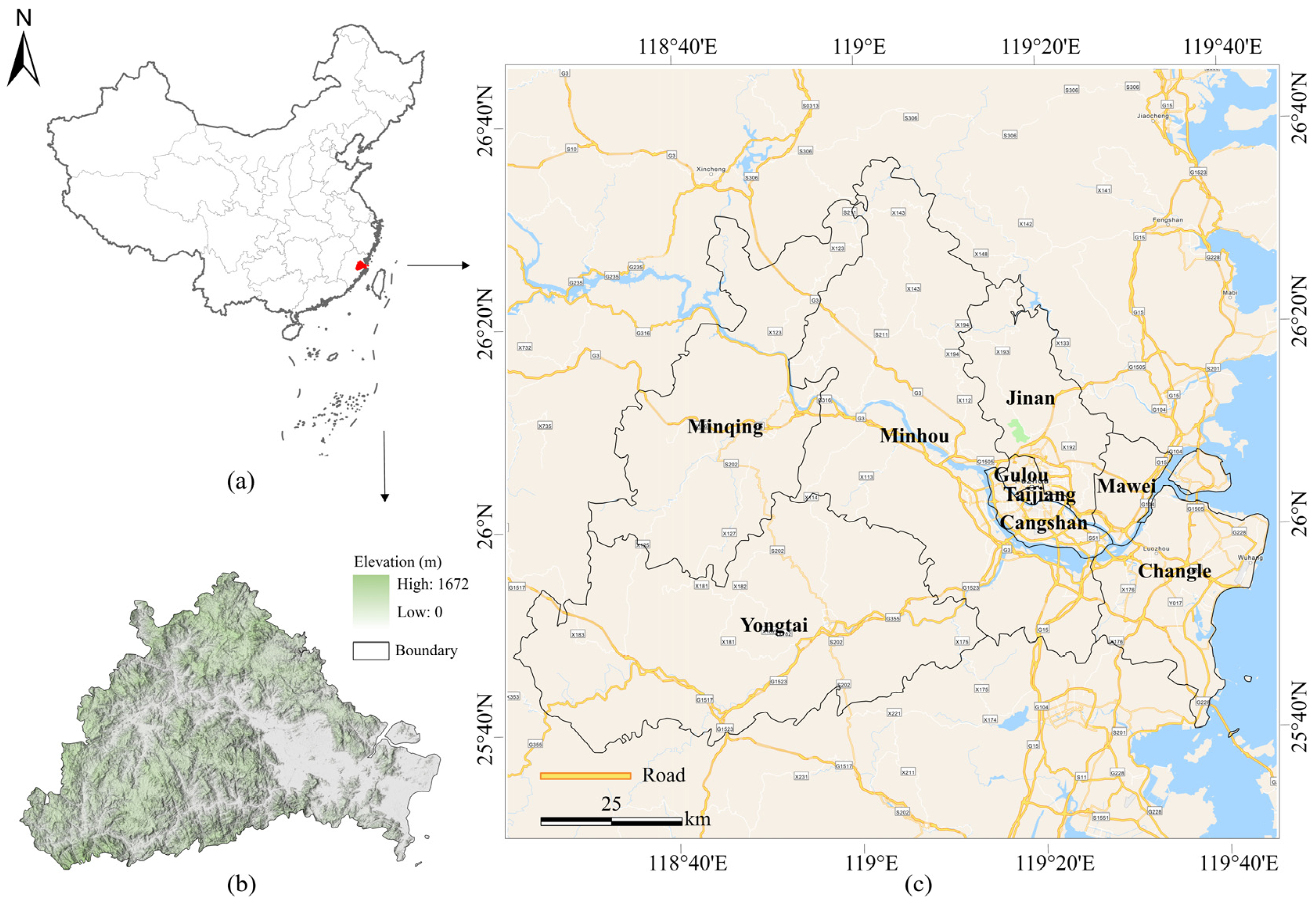
2.1. Study Area

Geographically, Fuzhou is situated on the southeastern coast of China, near the Taiwan Strait. The region is characterized by low mountains, hills, and plains, spanning approximately 12,000 km2 (Figure 1). This terrain is typical of southeastern China, making Fuzhou a strategic choice for studies providing insights and recommendations for both the city and the broader region. By the end of 2023, the total road length in Fuzhou City reached 11,749 km, with a road density of 106.5 km per hundred square kilometers. This includes 1279 km of national and provincial roads and 9706 km of rural roads, such as county, township, and village roads [37]. Fuzhou City, characterized by its extensive road network, is a representative region in China. It is renowned as one of the country’s new four major ’furnace’ cities [32,38]. The central urban area of Fuzhou is the most densely populated and economically developed region in Fujian Province. Monitoring its ecological quality is essential for assessing urban sustainability [39].

2.2. Data Sources and Preprocessing

Figure 2 illustrates the research method process and results framework. Data pre-processing supported the analyses of spatiotemporal dynamics and spatial patterns of the study area. A multi-scale sample unit design was employed, and spatial correlation along with driving factor analyses were conducted to determine the optimal scale. Subsequently, key driving factors were further examined.
The datasets used in this research primarily comprised Landsat imagery, road vector data, and driving factor datasets.
Regarding the Landsat remote sensing imagery, three periods were examined: 4 May 2000 (ETM+), 25 June 2016 (OLI/TIRS), and 27 September 2021 (OLI/TIRS). The imagery, acquired from the Computer Network Information Center of the Chinese Academy of Sciences (https://www.gscloud.cn/, accessed on 3 March 2023), underwent systematic geometric correction. The temporal resolution was 16 days, and the spatial resolution was 30 m. The cloud cover remained consistently below 10%. Preprocessing operations, such as image registration, radiometric calibration, cloud masking, and atmospheric correction, were performed using ENVI 5.6 [24,40]. Notably, the study area within the Minjiang River Basin contained numerous water bodies. To minimize the influence of water bodies on subsequent RSEI calculations, a modified normalized difference water index was employed to mask water areas [41].
OpenStreetMap provides highly comprehensive global geospatial data, which has been widely utilized in various studies [42,43]. The high-resolution data from OpenStreetMap is particularly valuable for examining the road network at the street level [44]. The road network vector data were downloaded from the OSM database (https://www.geofabrik.de/data/, accessed on 3 March 2023). Due to data availability limitations, this case focused on analyzing road network data for the years 2016 and 2021. To ensure data accuracy, selected roads underwent topological checks, and a consolidation tool was employed to merge two-lane roads and avoid duplicate calculations for the same road [32]. The preprocessed road vector data were used for KDE.
Moreover, to explore the multi-scale coupling relationship between the road network and ecological quality and further investigate the driving mechanisms of spatiotemporal changes in ecological quality, we considered an additional 12 driving factors. These factors were categorized based on their attributes into terrain, meteorology, ecology, and human activities [25,45,46,47] (Table 1).
The criteria for selecting these drivers are closely linked to the road network and ecological quality, and include the following: (1) Topographical factors such as elevation and slope significantly influence road construction and vegetation distribution [48]. (2) Meteorological factors like temperature and precipitation are critical drivers that impact environmental quality [45]. Additionally, PM2.5, a significant pollutant, contributes to environmental degradation within transportation systems [49]. (3) Within the ecological domain [23,50], our study includes fractional vegetation cover [51] and gross primary productivity [52]. These factors are essential for evaluating the impacts of land use and carbon balance. (4) Human activities transform landscapes through the creation of impervious surfaces such as buildings and transportation infrastructure, leading to irreversible environmental damage [53]. The distance from infrastructure serves as a measure of human impact on the environment [54]. Population density and gross domestic product [46] are validated as critical drivers of environmental impact. Notably, the normalized difference urban index is considered to gauge urbanization levels [55]. Lastly, all spatial data were transformed into the WGS_1984_UTM_ Zone_50N projection coordinate system and resampled to a spatial resolution of 30 m. These data processing tasks were primarily performed using ArcGIS 10.7.

2.3. Calculation of RSEI

RSEI possesses the ability to rapidly assess regional ecological environmental quality at various spatial and temporal scales [24]. In this study, ENVI 5.6 was used to extract four ecological indicators, namely the normalized difference vegetation index, normalized difference built-up index, land surface moisture, and land surface moisture, from three periods of remote sensing images in the study area: 2000, 2016, and 2021. The detailed calculation formulas can be found in Table S1. RSEI, synthesized using principal component analysis and based on the pressure-state-response framework and the four ecological indicators, is standardized within the range of [0, 1] to facilitate comparisons across different time periods. Higher RSEI values indicate better ecological quality, while lower values indicate poorer ecological quality [24,56]. The RSEI is primarily calculated through ENVI 5.6’s analytical modules, including radiation calibration, atmospheric correction, and principal component analysis (PCA).

2.4. Kernel Density Estimation

KDE is a valuable method for examining the spatial structure and impact of the road network. It calculates the density of features within their surrounding areas, providing insights into the characteristics of the road network [18,57]. Mathematically, the density at a location x is estimated as:
f ^ ( x ) = 1 n h 2 i = 1 n   K x x i h
where n is the number of features, h is the bandwidth, and K is a kernel function. The bandwidth of the kernel function, determined by a moving window, plays a crucial role in kernel density estimation [58]. A larger bandwidth leads to smoother and more diffused raster outputs, while a smaller bandwidth generates sharper and more detailed raster outputs. Therefore, we adopted Silverman’s rule of thumb, implemented in ArcGIS 10.7, to determine the optimal bandwidth and correct spatial outliers [59]. The KDE is implemented via the dedicated geostatistical toolbox in ArcGIS.

2.5. Buffer Analysis

Buffer analysis is employed to examine the spatial patterns of the interaction between road network development and ecological quality [60] and to conduct urban–rural gradient analysis [61]. In this research, to investigate gradient variations between urban and rural areas, the coordinates (latitude and longitude) of each district and county in Fuzhou City were obtained using Google Earth. Administrative centers were created as point features in ArcGIS 10.7, and three types of administrative centers were generated by aggregating all districts, all regions, and all counties. From each administrative center, thirty circular buffers with a radius of 1 km were created as point study objects. Within each buffer zone, we calculated the mean values of KDE and RSEI, allowing us to explore urban–rural differences from the perspective of urban centers.

2.6. Profile Analysis

Profile analysis is a quantitative method utilized for analyzing landform change [62]. In this study, the profile tool (3D Profile) in ArcGIS was employed to visualize the results of profile lines. A profile line represents a linear mark traversing the area of interest, while the profile plot depicts the variations of features along that line. To capture urban–rural gradient variations in KDE and RSEI, profile lines were established along three directions: north–south (N-S), southeast-northwest (SE-NW), and southwest-northeast (SW-NE). The selection of these directions was based on the distribution of administrative centers in each district and county.

2.7. Sample Unit Design

The modifiable area unit problem (MAUP) is worth considering when dealing with remote sensing data and conducting GIS analysis [63]. MAUP refers to the sensitivity of analysis results to data units, which can manifest as scale effects in landscape ecology [64,65]. When conducting spatial analysis within the same region, it is essential to consider the scale effect arising from spatial correlation [45], driving mechanisms [66], and spatial heterogeneity [67]. These factors can introduce variations in research outcomes across different scales. To address these variations, this study adopted a multi-scale approach by generating fishnet grids with sizes of 1000 m, 1500 m, 2000 m, 2500 m, and 3000 m. The sample sizes for these scales were 5897, 2605, 1477, 944, and 655, respectively. This approach enables a comprehensive investigation of the research area at different scales. Multi-scale analysis addresses these scale effects by characterizing MAUP to identify optimal scales. Spatial autocorrelation, GD, and regression analysis will employ the same sample unit design to explore the scale effect.

2.8. Spatial Autocorrelation Analysis

The core functionality of spatial autocorrelation analysis is to explore the spatial distribution characteristics of a variable and the degree of clustering among variables. It can be divided into global spatial autocorrelation and local spatial autocorrelation based on the research scale [68]. At the global scale, univariate global spatial autocorrelation is employed to analyze the spatial clustering of both KDE and RSEI. The global Moran’s I is defined as:
I = n W i = 1 n   j = 1 n   w i j ( x i x ¯ ) ( x j x ¯ ) i = 1 n   ( x i x ¯ ) 2
where n is the number of spatial units, x i is the attribute value at location i , x ¯ is the mean of x , w i j the spatial weight between units i and j , and W = i   j   w i j .
At the local scale, the study utilizes the local indicators of spatial association (LISA) for bivariate spatial autocorrelation analysis to investigate the spatial relationship between KDE and RSEI for both static and dynamic (Δ) patterns. The local Moran’s I for a univariate case is given by:
I i = ( x i x ¯ ) m 2 j = 1 n   w i j ( x j x ¯ )
where m 2 = 1 n i = 1 n   ( x i x ¯ ) 2 . For the bivariate case, where x represents KDE and y represents RSEI, the local Moran’s I is modified as:
I i = ( x i x ¯ ) m 2 , x j = 1 n   w i j ( y j y ¯ )
With m 2 , x = 1 n i = 1 n ( x i x ¯ ) 2 .
The results are assessed using Moran’s I index for correlation, z-scores for clustering, and p-values for significance. Both spatial autocorrelation analyses are conducted using GeoDa 1.22 (Spatial Data Science Center, University of Chicago, IL, USA). The specific procedures involve generating Rook adjacency spatial weights, setting a significance level (p = 0.05), and performing 999 permutation tests to assess sensitivity [69].

2.9. Geographical Detectors

GD are employed to study the driving mechanisms by exploring the spatial heterogeneity between ΔRSEI (Y) and explanatory factors(X). Four types of detectors are available: factor detectors, interaction detectors, risk detectors, and ecological detectors [70]. In the research, factor detectors and interaction detectors were selected to investigate spatial variations. The core function of factor detectors is to quantify the spatial heterogeneity between ΔRSEI (Y) and individual explanatory factors(X), thereby revealing the relative importance of different explanatory factors. This is primarily accomplished through the calculation of the q -statistic (hereafter denoted as q ), which is defined as follows:
q = 1 j = 1 W N g σ g 2 N σ 2
where j = 1,…, W represents the number of stratification levels; N g and N represent the number of spatial units in the gth layer and all layers, respectively; σ g 2 and σ 2 are the variances of Y in the g layer and all layers, respectively. A higher q -statistic indicates a stronger spatial heterogeneity of ΔRSEI (Y) and a higher explanatory power of the explanatory factor (X). The q -statistic ranges from 0 to 1.
Interaction detectors are tools to determine the joint driving effects of any two explanatory factors on ΔRSEI. By comparing the q -statistic (X1 ∩ X2) generated by the interaction of X1 and X2, the explanatory power of different combinations of explanatory factors on the dependent variable ΔRSEI (Y) can be assessed. According to the interaction detection, the results are usually divided into six types: enhance; bivariate-enhance; nonlinear-enhance; weaken; univariate-weaken; nonlinear-weaken; independent [70].

2.10. Global and Local Regression Models

Linear regression techniques have long been utilized as an analytical tool by quantitative geographers to study the relationships between geographic variables [71]. Compared to ordinary least squares (OLS), GWR provides additional insights into spatial parameters. It assumes that all explanatory variables share the same neighborhood and explores interesting spatial details in the relationships by running the model at the same spatial proportion of local relationships. The GWR model is formulated as:
y i = β 0 u i , v i + k = 1 p   β k u i , v i x i k + ε i
where ( u i , v i ) represents the spatial coordinates of observation i , β k ( u i , v i ) are the local regression coefficients estimated at each location, and εi\varepsilon_iεi is the error term. The coefficients β k ( u i , v i ) are estimated using a spatial weighting function, typically based on a Gaussian or adaptive kernel, where observations closer to location ( u i , v i ) have a greater influence on the local estimates.
Compared to GWR, MGWR provides separate neighborhoods for each explanatory variable and different spatial proportions for different explanatory variables. The MGWR model is expressed as:
y i = β 0 ( u i , v i ; h 0 ) + k = 1 p   β k ( u i , v i ; h k ) x i k + ε i
where h k denotes the bandwidth specific to explanatory variable x k , enabling different variables to exert influence over varying spatial extents. This flexibility enables MGWR to generate different bandwidths and more accurate estimates of local regression coefficients [67].
This research employed global models (OLS) and local models (GWR, MGWR) to explore the spatial patterns and driving mechanisms of ecological quality change in relation to explanatory variables. To assess multicollinearity, the OLS model was used to identify explanatory variables with a variance inflation factor (VIF) greater than 5 and those that did not pass the significance test [72]. The GWR and MGWR models were implemented using the MGWR 2.2 software, based on Python [73]. Model evaluation was performed using multiple parameters, including R-squared, adjusted R-squared, the corrected Akaike Information Criterion (AICc), residual sum of squares, residual Moran’s I, and effective number of parameters.
For the local models, we compared the spatial distribution of R-squared values at different scales to identify the optimal scale for each model. Additionally, we compared the optimal bandwidths derived from GWR and MGWR, and further analyzed the spatial distribution of MGWR coefficients, including their mean values and the proportions of positive and negative coefficients.

3. Results

3.1. Urban–Rural Gradient Patterns in Road Networks and Ecological Quality

Figure S1 presents the spatiotemporal dynamics of the road network in Fuzhou City for the years 2016 and 2021. The findings reveal a gradient shift in the distribution of KDE within Fuzhou City, exhibiting notable spatial variations. In both 2016 and 2021, high KDE values were predominantly concentrated in urban areas, gradually decreasing as they moved away from the city center. Regarding temporal changes, the average KDE value increased from 0.886 km/km2 in 2016 to 1.646 km/km2 in 2021, representing an increase of 0.759 km/km2, which suggests coordinated growth in both urban and rural road networks. Remarkably, substantial growth was observed near the Changle District and Minhou County, situated at the urban–rural interface.
Additionally, Figures S2 and S3 illustrate the spatial patterns and dynamic changes in ecological quality, respectively. The RSEI predominantly declined from 2000 to 2016 but showed an improvement trend from 2016 to 2021. Changes in RSEI reflected significant urban–rural differences, with a decline from 2000 to 2016, followed by an increase from 2016 to 2021. Improvements in ecological quality exhibited a trend of gradually increasing from the urban center to rural areas, with notable fluctuations particularly concentrated in districts such as Gulou, Cangshan, and Changle, and their interfaces with Minhou County.
Overall, along the urban–rural gradient (Figure S4), we observed varying patterns of change in the KDE and RSEI curves. The KDE curve decreased with increasing distance from the administrative centers, while the RSEI curve exhibited an increasing trend. Both curves gradually flattened after reaching a certain threshold, indicating a “gradient” characteristic with minor fluctuations. Specifically: (1) When analyzing all districts and counties, the KDE curve began to level off after 15 km from the administrative center and remained stable within a range of up to 25 km. Slope analysis showed a greater decrease in the KDE curve in 2021 compared to 2016 within the 0–5 km range from the administrative center. The RSEI curve, on the other hand, started to level off after 25 km from the administrative center. Within the 15–25 km range, the 2021 RSEI curve appeared smoother compared to 2016 and 2000. (2) Focusing on district-level administrative centers, which were relatively concentrated, the spatial superimposition effect of multiple circular buffers was more pronounced. The KDE curve exhibited a flatter trend after 25 km from the administrative center, with a slight increase at 22 km. The RSEI curve showed more intricate changes, generally increasing within the 25 km range from the administrative center. However, the RSEI curve showed a decrease within the 2 km range, followed by an increase, a decrease at 19 km, and a subsequent continuous increase, with a downward trend after 25 km. (3) Examining county-level administrative centers, the KDE curve leveled off after 10 km, with a turning point at 11 km in 2016. The upward trend of the RSEI curve also flattened after 10 km, with a minor decrease in the 15–30 km range in 2000. The urban–rural gradient characteristics were more prominent within this range.
Comparing the KDE and RSEI values across the three scenarios, we found that KDE values in urban areas were significantly higher than those in county towns, while RSEI values in county towns were higher than in urban areas, reflecting urban–rural differences.
Analysis of the KDE profile plots crossing the administrative centers (Figure S5) revealed higher KDE values in the central area, followed by neighboring districts and counties, with lower values in areas farther from the central region. In the SE-NW and SW-NE directions, the KDE profile forms a “peak” in the central area, reaching its maximum value. As the distance from the central area increases, the KDE values decrease, forming “valleys” and reaching low values.
The RSEI profile plots (Figure S6) showed lower RSEI values when passing through different administrative centers compared to the surrounding areas along the three directions. Regarding temporal changes, RSEI values decreased from 2000 to 2016 and recovered to higher levels in 2021, especially in the N-S and SW-NE directions. Analyzing the trend of curve changes, the RSEI in the SE-NW direction significantly declined in 2016 but showed remarkable improvement in 2021. Additionally, the RSEI in the N-S and SW-NE directions was better than that in the SE-NW direction, with areas of higher RSEI mainly concentrated in the periphery of county seats and urban–rural transition zones.

3.2. Univariate Global Spatial Autocorrelation Analysis of Road Networks and Ecological Quality at Multi-Scale

To account for the potential impact of spatial scale on our research findings, this study examined the spatial relationship between the KDE and RSEI using five different grid cell sizes: 1000 m × 1000 m, 1500 m × 1500 m, 2000 m × 2000 m, 2500 m × 2500 m, and 3000 m × 3000 m. The results of the global spatial autocorrelation analysis (Table S2) indicate a significant scale effect in spatial correlation and aggregation (p-values). Specifically: (1) For static KDE, the Moran’s I index exceeds 0.92 at the 1500 m and 2500 m scales, indicating a high correlation. However, at the 2000 m scale, the Moran’s I index is only 0.46, indicating a low correlation. This nearly twofold difference suggests that the spatial distribution of KDE does not exhibit a monotonic relationship with scale. Additionally, the observation of z-scores reveals that the maximum z-score occurs at the 1000 m scale, indicating the highest level of spatial clustering. However, at the 2000 m scale, although the z-score is relatively high, the Moran’s I index is low, indicating a high level of spatial clustering but insignificant correlation. This result suggests that the spatial correlation and aggregation of KDE do not exhibit a completely monotonic change. (2) For static RSEI, the Moran’s I index indicates a significant scale effect in spatial correlation, with the highest correlation at the 1500 m scale and the lowest at the 3000 m scale. The z-scores suggest a weak scale effect in spatial clustering, with the highest level of spatial clustering at the 1000 m scale and a lower level at the 2000 m scale compared to the 1500 m and 2500 m scales.

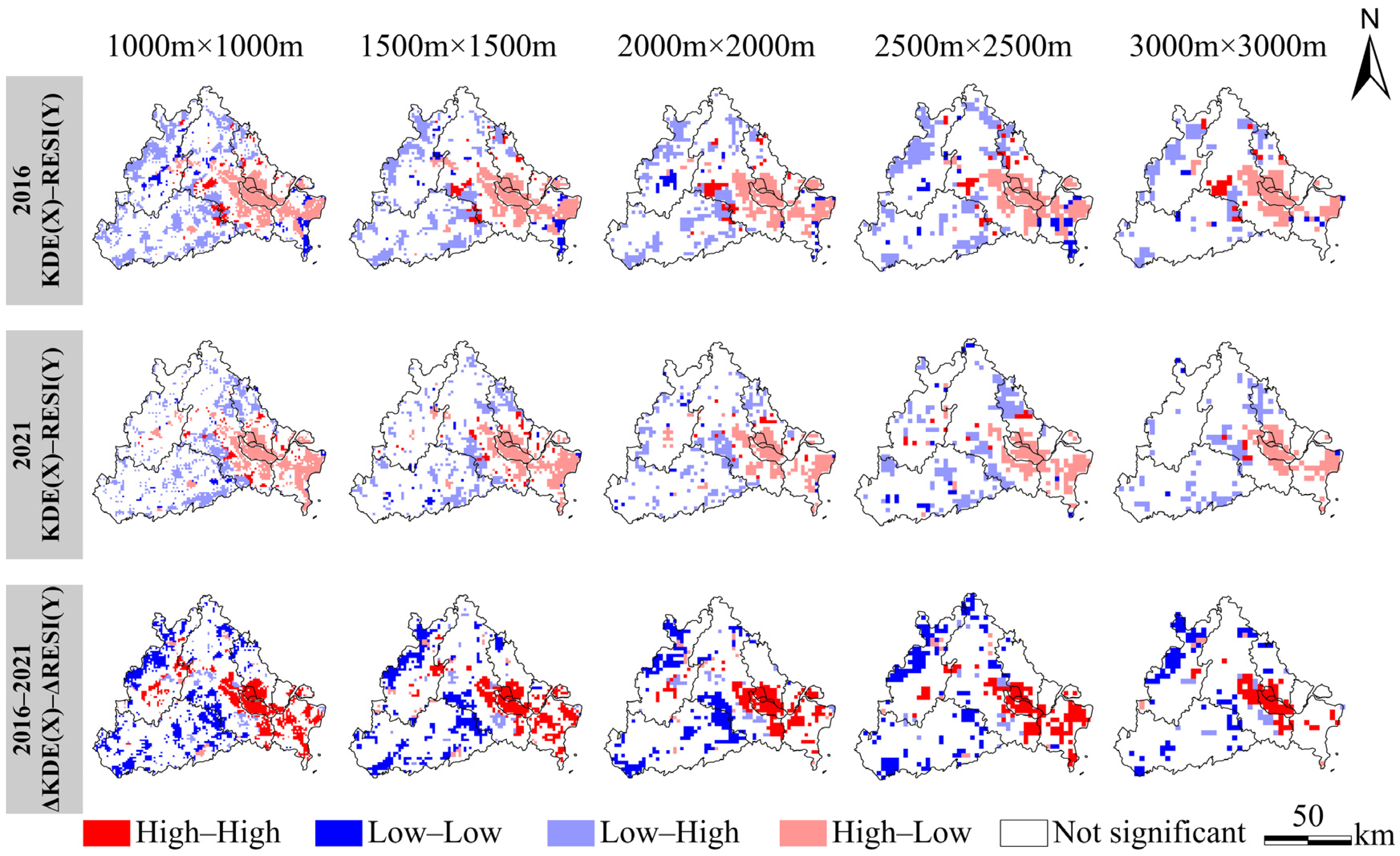
3.3. Spatiotemporal Coupling Relationships of Road Networks and Ecological Quality at Multi-Scale

To explore the local spatial relationship between KDE and RSEI at various scales, including negative (i.e., tradeoff) and positive (i.e., synergistic) relationships, we employed LISA analysis to assess local spatial correlations and identify significant hotspots and cold spots. The analysis period spanned from 2016 to 2021, and three sets of bivariate data were examined: 2016 KDE and RSEI, 2021 KDE and RSEI, and the dynamics in ΔKDE and ΔRSEI. The results indicate significant findings at all scales (Table 2), passing the 0.1% significance test (p-values). The Moran’s I index and z-scores exhibited an increasing trend from the 1000 m scale to the 3000 m scale, suggesting a significant spatial clustering pattern rather than random distribution. Specifically, (1) in 2016 and 2021, negative values of Moran’s I index were observed at all scales, indicating a tradeoff relationship between KDE and RSEI. However, the z-scores indicated a relatively dispersed spatial distribution. (2) Regarding the analysis of dynamic patterns, positive correlations were observed at all scales for the period from 2016 to 2021, describing a synergistic relationship between ΔKDE and ΔRSEI. The highest correlation was observed at the 1000 m scale with a Moran’s I index of 0.393, while the lowest was at the 3000 m scale with a Moran’s I index of 0.265. Notably, the Moran’s I index value for 2016–2021 was 0.385 at both the 1500 m and 2000 m scales, but their z-scores were not equal. Considering the z-scores, where 52.586 > 38.444, it indicates that the 1500 m scale is associated with a larger number of spatial units than the 2000 m scale, suggesting a higher level of clustering between the ΔKDE and ΔRSEI at the 1500 m scale.
We conducted a bivariate LISA cluster analysis to assess the spatial distribution (Figure 3) and examine the local spatial relationships between KDE units (X) and RSEI units (Y). However, the LISA clustering results for static KDE-RSEI and dynamic ΔKDE-ΔRSEI during 2016–2021 exhibited markedly different patterns. Specifically: (1) The multi-scale analysis revealed that as the scale decreased from 3000 m to 1000 m, the local spatial patterns became more detailed, with a notable increase in High-Low and Low-High regions, along with a slight rise in High-High and Low-Low regions. At finer scales (1000 m and 1500 m), the spatial patterns exhibited greater heterogeneity, with High-Low and Low-High regions becoming more fragmented and widely distributed. In contrast, at coarser scales (2500 m and 3000 m), these regions were more aggregated, and spatial transitions between cluster types appeared smoother. (2) The static spatial clustering results for 2016 and 2021 predominantly showed High-Low and Low-High situations. Urban areas were primarily associated with High-Low regions, while county towns exhibited a concentration of Low-High regions. In particular, High-Low clusters were concentrated in urban districts such as Gulou, Cangshan, and Changle, whereas Low-High clusters were more prominent in the surrounding county towns, including parts of Minhou and Minqing. The spatial extent of these clusters varied slightly depending on the scale, with finer resolutions capturing more localized variations. (3) The dynamic clustering results for changes from 2016 to 2021 predominantly displayed High-High and Low-Low regions, indicating strong correlation and aggregation. High-High hotspots of changes in ΔKDE and ΔRSEI were mainly concentrated in the urban–rural interfaces, showing a high degree of spatial clustering and significant changes. These were particularly evident at the intersections of Gulou, Cangshan, and Changle districts with Minhou County, where High-High clusters consistently appeared across multiple scales, highlighting areas experiencing simultaneous increases in KDE and RSEI. Additionally, sporadic High-High clusters were observed at the borders of Minhou and Minqing counties, albeit with slightly lower spatial persistence across scales. Meanwhile, Low-Low cold spots of changes were mainly located at the periphery of county towns, indicating scattered distribution and relatively stable environmental conditions, particularly in the northeastern part of Yongtai County and the northwestern part of Minqing County. These Low-Low clusters exhibited more fragmented patterns at finer scales (1000 m), whereas at coarser resolutions, they formed more contiguous zones, suggesting the persistence of relatively stable environmental conditions in these areas. (4) From a spatiotemporal analysis perspective, the period from 2016 to 2021 demonstrated the optimal level of spatial clustering and significance, with the 1000 m scale providing the most accurate reflection of local characteristics in changes in ΔKDE and ΔRSEI.

3.4. Driving Patterns of Road Network on Ecological Quality

3.4.1. Individual and Interactive Effects of Road Network on Ecological Quality

To investigate the key factors influencing ΔRSEI, a GD analysis was conducted. The results (Table 3) indicate significant variations in explanatory power and importance across different scales. The cumulative explanatory power (total of q-statistic) shows that the sum of explanatory power for each driving factor is highest at the 3000 m scale and lowest at the 1500 m scale, with values at the 2000 m and 1000 m scales being similar. In the context of single-factor analysis for ΔKDE, all factors achieved a ranking of 4 out of 13, with only dynamic (Δ) factors ranking 2 out of 9, indicating strong explanatory power. Terrain factors (e.g., elevation and slope) show the highest explanatory power in terms of mean values, followed by ΔPM and ΔKDE, associated with human transportation activities, significantly impacting ΔRSEI. However, ecological factors such as ΔGPP and ΔFVC have the lowest explanatory power and less influence on ΔRSEI, possibly due to slower vegetation growth rates compared to the frequency of human activities. Additionally, the cumulative significance results (p-values) indicate that at the 3000 m and 2500 m scales, the dynamics in ΔGPP, ΔNDUI, ΔFVC, and ΔPD are not significant. However, at the 2000 m and 1500 m scales, only ΔNDUI is not significant, and at the 1000 m scale, all factors are significant. Thus, the lower significance of these four factors at larger scales reflects the influence of scale effects.
The interaction detection (Figure 4) between ΔKDE and other factors concerning ΔRSEI reveals mainly a bivariate enhancement and a slight nonlinear enhancement relationship, both demonstrating higher explanatory power than ΔKDE’s single-factor effect. The multi-scale mean values indicate that the interaction of ΔKDE with elevation and slope is the strongest, reaching 0.256 and 0.255, respectively. Following closely are ΔPM, DURRP, and ΔPD, indicating favorable interactions with ΔKDE concerning terrain factors and human activities. Interestingly, changes in ΔNDUI and ΔLST show a nonlinear enhancement of ΔKDE at both 2500 m and 3000 m scales, with both having a multi-scale mean of 0.190.
The interaction detection results (Figure 4) reveal variations in the explanatory power of interactions at different scales. Mean values of the explanatory power of multi-scale interactions indicate that elevation, slope, ΔKDE, and ΔPM have strong shared explanatory power with other driving factors, while ΔLST and ΔPREC have weaker shared explanatory power. At the 3000 m scale, interactions of each driving factor have the strongest explanatory power, ranging from 0.042 to 0.338. Among the different interaction combinations, elevation and slope exhibit the highest shared explanatory power, followed by ΔPM and slope, and ΔKDE and slope. However, meteorological factors like ΔLST and ΔPREC show weaker shared explanatory power with other driving factors. Notably, the shared explanatory power of ΔKDE was lower at the 3000 m scale compared to other scales, while it demonstrated strong shared explanatory power at the 1500 m and 2500 m scales. Specifically, ΔKDE displayed significant interactions with elevation, DURRP, and DTAFP. The results of spatial stratified heterogeneity in interaction detection indicated that terrain distribution had a significant influence on improving ΔRSEI, followed by changes in human activities, while the contribution of meteorological factor changes was relatively small.

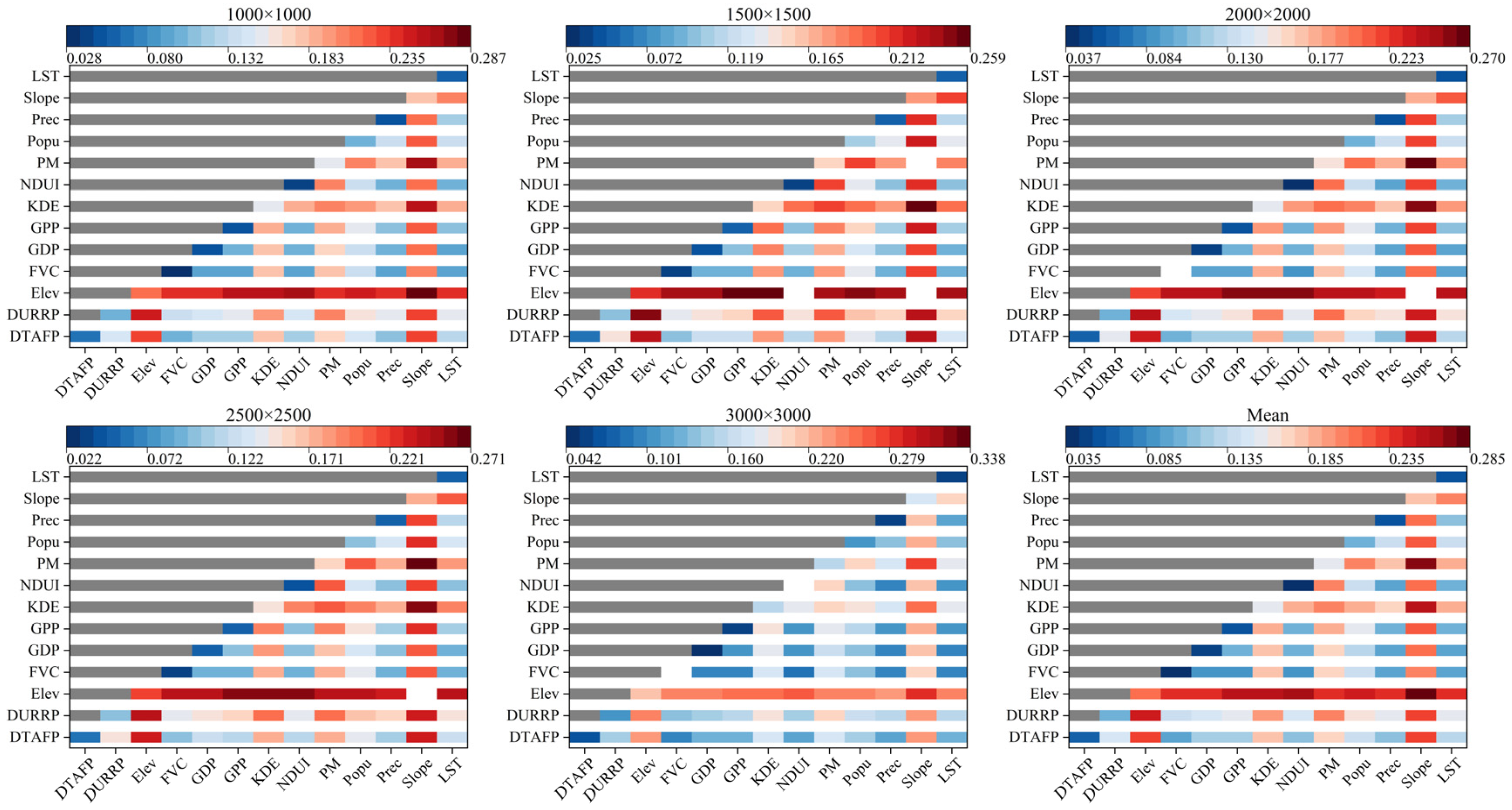
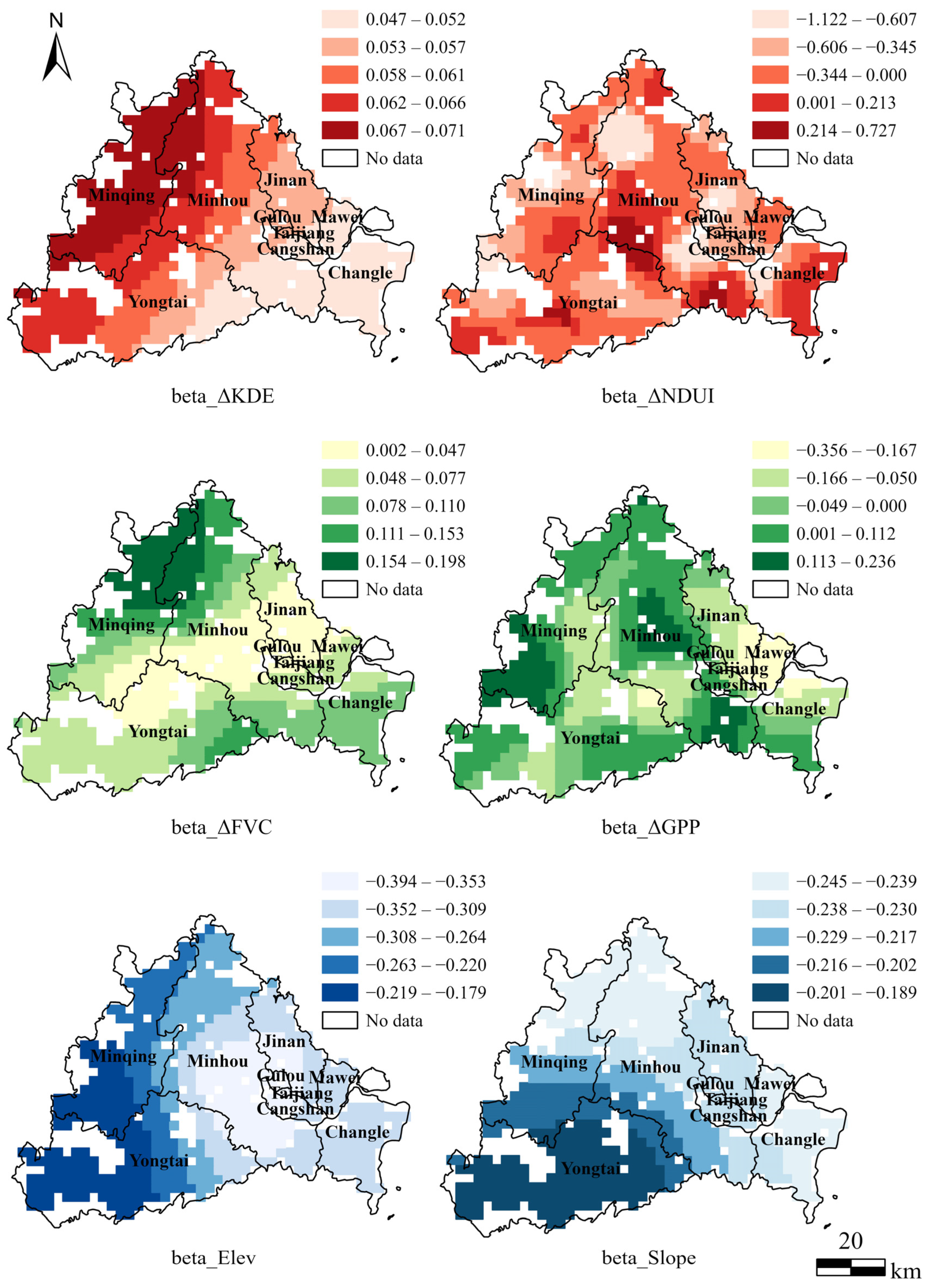
3.4.2. Spatial Variations in the Driving Patterns of Road Network on Ecological Quality

To address multicollinearity, we conducted exploratory spatial data analysis, running OLS models on each possible combination of explanatory variables. The results of the multi-scale exploratory regression analysis (Table S3) indicate that all driving factors at different scales have VIFs below 5, passing the multicollinearity test.
Then, we applied the global regression OLS model, the local regression GWR model, and the MGWR model to the driving factors at different scales. The regression analysis results are presented in Table 4, demonstrating the superiority of the local regression and MGWR models over the global regression and GWR models, respectively. The key observations are as follows: (1) The MGWR model shows the highest R-squared and adjusted R-squared values, indicating a better fit to the data. (2) The MGWR model has the lowest AICc and residual sum of squares values, indicating higher predictive accuracy. (3) The residual Moran’s I value for the local models is lower than that of the global model, suggesting a random distribution of residuals and more reliable results.
Superior results were observed for MGWR. The bandwidth comparison results (Figure 5) indicate that the MGWR model can directly reflect the unique bandwidths of different driving factors, whereas the GWR model can only capture the average bandwidths of different driving factors. Furthermore, the bandwidths vary across different spatial sample units (SSUs), and scale changes are accompanied by changes in sample size. The bandwidth range of the GWR model changes from 393 SSUs to 521 SSUs, while the bandwidth range of the MGWR model varies from 44 SSUs to 5896 SSUs, indicating a significant difference. Specifically, (1) in GWR, the bandwidth of ΔKDE is the same as that of other driving factors, while in MGWR, it varies. At the 1500 m scale, the bandwidth of ΔKDE is 497 SSUs, indicating a relatively small influence range. In contrast, at other scales, the bandwidth of ΔKDE extends to the global scale, suggesting a larger influence range compared to most driving factors. (2) At the 1000 m scale, ΔNDUI and ΔGPP exhibit limited bandwidths of 70 and 416 SSUs, respectively, corresponding to 1.19% and 7.05% of the total sample size. Conversely, ΔKDE and DURRP demonstrate a global influence, encompassing 5896 SSUs, nearly 100% of the bandwidth. At the 3000 m scale, ΔNDUI and ΔGPP show bandwidths of 44 and 103 SSUs, accounting for 6.73% and 15.75%. Similarly, ΔKDE and slope maintain a global reach, with a bandwidth of 654 SSUs, close to 100%. (3) Lastly, changes in ΔFVC, ΔNDUI, and ΔPD exhibit pronounced spatial heterogeneity across all scales, while changes in ΔPM and ΔPREC have bandwidths close to the global scale at all levels, indicating minimal spatial heterogeneity.
Figure 6 shows the spatial distribution of local goodness of fit for the GWR and MGWR models. The MGWR model demonstrates superior fitting results, especially at the 3000 m scale. In this case, we aimed to explore the driving mechanisms behind the improvement of ΔRSEI by conducting a multi-scale analysis using the significant (p < 0.05) driving factors identified through OLS tests (Table S3). Therefore, we selected six driving factors: dynamics in ΔKDE, ΔNDUI, ΔFVC, ΔGPP, and static elevation and slope to examine their spatial patterns in the MGWR model regression coefficients at the 3000 m scale.
The regression coefficients of the variables exhibit spatial heterogeneity and gradient characteristics between urban and rural areas, impacting ΔRSEI to varying degrees (Figure 7). Positive correlation coefficients indicate synergies, whereas negative coefficients suggest tradeoffs. At the 3000 m scale, the spatial heterogeneity of regression coefficients suggests the following patterns: (1) ΔKDE shows synergy with ΔRSEI, presenting a gradient change that weakens from the northwest county areas towards the southeast urban areas, with strong synergies in Minqing, Minhou, and Yongtai counties, and the weakest in Mawei and Changle districts. Conversely, ΔNDUI exhibits both tradeoff and synergy regions, with tradeoffs accounting for 75.88% and synergies for 24.12% (Figure 8a). Tradeoffs mainly occur in urban centers, particularly in Cangshan and Taijiang districts, while synergies are mainly found in suburban areas, such as the interface of Minhou and Yongtai counties. (2) For ecological factors, ΔFVC shows a synergy effect, with high values concentrated at the interface of Minqing and Minhou counties and weaker effects near Gulou District. However, ΔGPP has nearly equal proportions of tradeoff and synergy regions, accounting for 48.24% and 51.76% respectively. Tradeoffs are primarily found in Mawei District, while synergies are concentrated in central Minhou County and southwestern Minqing County. (3) Among the topographical factors, elevation shows a tradeoff effect, primarily affecting the ring area around Gulou District and its interface with Minhou County, weakening as it spreads outward. Slope also displays a tradeoff effect, increasing from the weakest in Yongtai County to higher levels towards the north. Among the six major driving factors (Figure 8b), road construction (e.g., ΔKDE) and ecological factors (e.g., ΔFVC and ΔGPP) primarily generate synergistic effects on ΔRSEI, while urbanization processes (e.g., ΔNDUI) and terrain factors (e.g., elevation and slope) primarily result in tradeoff effects on ΔRSEI.

4. Discussion

4.1. Changing Relationships Between Road Networks and Ecological Quality

The linear features constructed by humans connect us, but also fragment nature [74]. In this research, both buffer and profile analysis revealed a tradeoff relationship between KDE and RSEI. Observations of distinct peaks and valleys in the data show that RSEI values are lower near roads, while areas closer to the administrative center display higher KDE values and lower RSEI scores. These patterns may be associated with the ‘edge effect’, which refers to various biological and physical changes associated with roads and their surrounding areas, resulting in drier and hotter conditions closer to the edge and higher tree mortality rates [75,76,77,78]. However, the interaction of temporal variations indicated a synergistic relationship between the two factors according to local spatial autocorrelation analysis. This suggests that while road network expansion occurs, ecological quality improvement can also be achieved [79]. The potential reasons for the synergy between ΔKDE and ΔRSEI include coordinated urban–rural development, as observed at the urban–rural interfaces of Minhou County and the surrounding urban areas. Moreover, this phenomenon may be linked to vegetation recovery during the urbanization process, supported by previous studies that reported positive changes in tree cover in China’s urban core areas over the last two decades [80,81,82,83]. In summary, the evolving relationships between the road network and ecological quality unveil a complex interplay of tradeoffs and synergies.
Furthermore, it is noteworthy that correlation implies a specific type of association, which may result from direct or indirect reasons, such as monotonic trends or clustering, but not causation [84]. For instance, we observed a synergistic relationship between ΔKDE and ΔRSEI within the LISA clustering; however, this correlation does not imply causation. Similarly, our findings in GD’s interaction exploration indicate that other driving factors for ΔRSEI may exert both direct and indirect influences.
Understanding the balance and positive effects between human well-being and the environment is crucial for all issues [85]. Therefore, the GD was employed to explore the driving mechanisms of ΔRSEI at multiple scales. The results indicate that the ΔKDE is one of the highly influential driving factors for ecological quality change. From the perspective of interaction detection, ΔKDE exhibits enhancement effects at different scales; moreover, extremely rare nonlinear enhancement was observed in the interaction between ΔLST and ΔNDUI. This phenomenon may be related to the urban heat island effect during the urbanization process, and the ΔKDE could partly account for Fuzhou’s reputation as a “furnace”. Among these, ΔKDE has the strongest joint effects with topographical factors (e.g., elevation and slope) on ΔRSEI. Furthermore, across various scales and different regions, ΔKDE and ΔRSEI predominantly exhibit synergistic effects. The rational planning and design of roads can have environmental benefits [86], while local adaptation in spatial ecology can mitigate the effects of associated ecological change, explaining the recent improvements in ecological quality [87]. Meanwhile, in GWR, the bandwidth of ΔKDE remains the same as other driving factors, while in MGWR, variations are observed. At the 1500 m scale, the bandwidth of ΔKDE is 497 SSUs, indicating a relatively localized influence range. In contrast, at other scales, the bandwidth of ΔKDE extends to the global scale, suggesting a broader impact on ecological governance than most drivers.
To reveal the multiscale tradeoffs and synergies among the driving mechanisms, we analyzed the spatial distribution of the regression coefficients of the six driving factors in MGWR. The results indicate variations in the influence range of different factors, presenting a spatial gradient of heterogeneity. Specifically, ΔNDUI indicates that urbanization processes have a tradeoff effect on ΔRSEI, while ΔKDE suggests that road construction can establish a synergistic relationship with ΔRSEI. In the context of rapid urbanization in China and the increasing prominence of ecological civilization, our findings not only clarify the interactions between infrastructure development and ecological quality but also provide new insights for future policy formulation. While road expansion can lead to negative impacts such as habitat fragmentation and increased pollution, strategic interventions can simultaneously foster ecological improvements. For example, in urban–rural interface areas, targeted road ecological restoration initiatives, such as the construction of ecological corridors and roadside green belts, have been observed to mitigate habitat isolation and enhance local biodiversity, thereby counteracting some adverse effects of increased road density. These dual effects are in agreement with landscape ecology theories, which suggest that thoughtful spatial planning and ecological restoration can balance infrastructure expansion with environmental preservation. Based on these results, potential policy measures could integrate ecological restoration practices into road construction projects and establish environmental compensation mechanisms. These policy directions, supported by scientific evidence and practical significance, align with China’s ecological civilization goals.

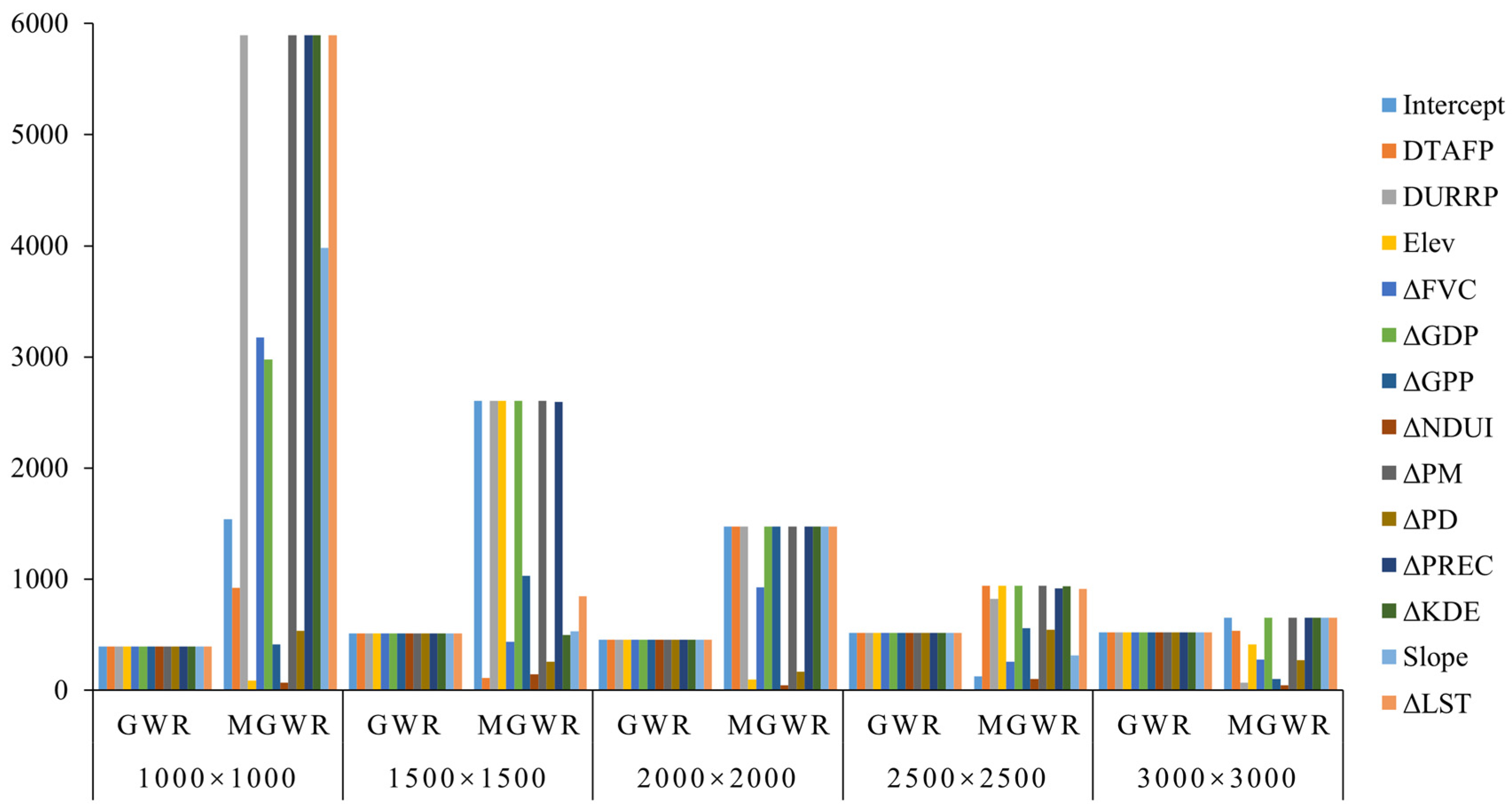
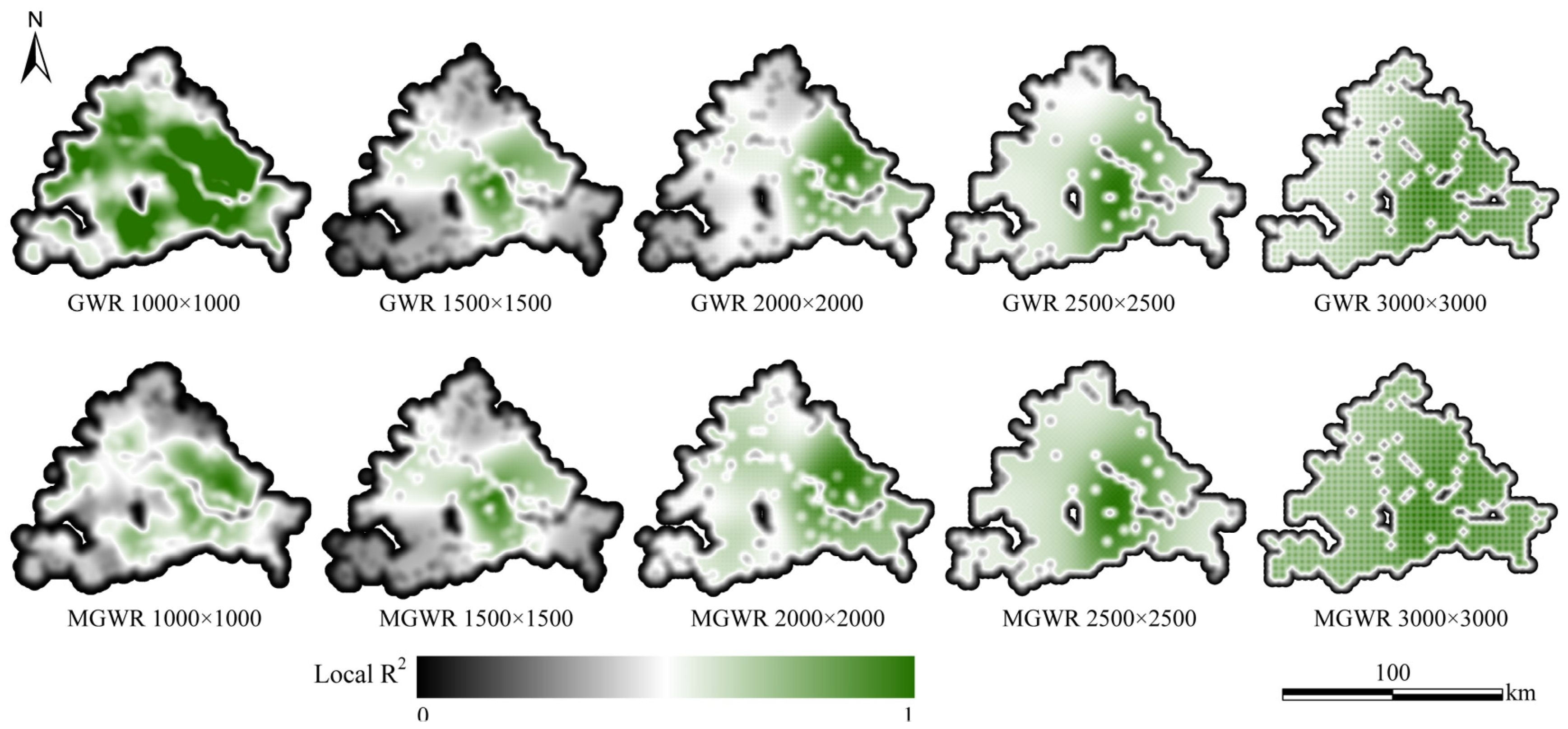
4.2. GD, GWR, and MGWR: Differences in Exploring Spatial Heterogeneity

Spatial heterogeneity, often referred to as the second law in geography, pertains to the statistical non-stationarity observed in geographic variables [88]. Here, we conducted a comprehensive analysis of spatial heterogeneity through different geographical models (e.g., GD, GWR, and MGWR). Significantly, we employed a well-established multi-scale sample design widely used in landscape ecology to investigate the scale effect within the context of the MAUP and to analyze driving mechanisms at the optimal scale. The combined use of GD, GWR, and MGWR across various scales facilitated a comprehensive exploration of driving mechanisms. GD effectively captures stratified heterogeneity through the calculation of the q statistic within the [0, 1] range, thereby illuminating underlying driving mechanisms. In contrast, GWR and MGWR excel in delineating process-based spatial heterogeneity using bandwidth and regression coefficients. Particularly, MGWR stands out in providing a more nuanced characterization of local heterogeneity due to its unique bandwidth design.
The complexity of geographic phenomena and processes goes beyond the spatial domain and extends to the interactions of driving factors [89]. Nonetheless, considering the primary focus of our study on investigating the multiscale interaction between ΔKDE and ΔRSEI, the interaction analysis of GD still displayed the highest explanatory efficacy at the 3000 m scale, indicating the attainment of the optimal scale for our inquiry. Furthermore, the interaction detection results reveal variations in multi-scale driving mechanisms. For instance, ΔKDE displays high co-explanatory power at the 1500 m and 2500 m scales but less at the 3000 m scale, indicating the presence of spatial heterogeneity across all scales [90].
It is important to note that most research focuses on the driving mechanisms of static factors at individual scales, while comprehensive MGWR studies on dynamic factors and multi-scale explorations are relatively sparse. The strengths and contributions of this study’s application of MGWR are as follows: First, local regression achieves optimal performance at the 3000 m scale, while MGWR outperforms GWR at different scales. This is likely due to MGWR’s unique bandwidth mechanism, which outperforms traditional GWR [91]. Second, the bandwidth reveals the scale effect of driving factors from the perspective of spatial heterogeneity, and MGWR can provide individual bandwidths for each driving factor [67,92]. The multi-scale results show that both scale and bandwidth change, as scale is a complex and multifaceted concept in geography, but in spatial statistics, it generally refers to bandwidth [93].
When scrutinizing driving mechanisms, GD excels in identifying interaction mechanisms among different explanatory factors through interaction detection. In contrast, GWR and MGWR excel in describing local spatial heterogeneity features and revealing the promoting or inhibiting roles played by distinct explanatory factors. The integration of these modeling approaches enhances the comprehensive understanding and identification of driving mechanisms.

4.3. Ecological Mitigation for Road Network Development

Our observations indicate that the ecological quality in Fuzhou City declined from 2000 to 2016, followed by an improvement from 2016 to 2021. This improvement, occurring alongside road expansion, suggests a complex relationship between ecological quality and the road network. For example, through bivariate spatial autocorrelation analysis, we uncovered a tradeoff relationship between static KDE and RSEI, while a synergistic relationship between ΔKDE and ΔRSEI. This synergistic effect was also confirmed through MGWR analyses, demonstrating its validity in terms of spatial autocorrelation and spatial heterogeneity. These findings establish strong correlations and are robust across multiple scales of sampling units, marking significant progress over previous studies. Overall, our study presents a novel finding that static relationships exhibit a negative correlation, while dynamic relationships show a positive correlation. This is significant for advancing understanding in the field of road ecology. This novel discovery supports the notion that thoughtful road expansion from 2016 to 2021 was compatible with ecological improvements. Such findings demonstrate the successful application of road ecology principles and suggest the potential for our observational approach to be extended to other regions.
Given that this study was conducted at a landscape scale, our findings have important implications for assessing the long-term ecological impacts of road networks. Specifically, the observed dynamic interactions between road expansion and ecological quality suggest that strategic modifications to road networks could mitigate negative ecological impacts over time. For instance, adjusting road alignments to reduce habitat fragmentation, lowering road density in ecologically sensitive areas, and incorporating ecological corridors into road planning may help lessen adverse impacts on ecological quality. These recommendations can be incorporated into national and local policies by aligning transportation planning with green infrastructure development, updating zoning regulations to prioritize ecological restoration, and fostering sustainable urban development in rapidly urbanizing regions.
Furthermore, these results hold practical significance for China’s comprehensive transportation hubs, underscoring the critical role of policies emphasizing ecological protection and restoration during road construction. In accordance with the “National Comprehensive Three-Dimensional Transportation Network Planning Outline” [15] and the latest “Fuzhou City 14th Five-Year Comprehensive Transportation Development Plan” [94], we further recommend: (1) Our RSEI analysis can identify areas of ecological restoration and degradation, which is a prerequisite for proposing protection and restoration strategies. The results for Fuzhou City suggest that the Gulou, Cangshan, and Changle districts require restoration efforts (Figures S2 and S3), particularly at their urban–rural interfaces with Minhou County, while other areas should focus on ecological protection. (2) Using LISA and MGWR, we can identify the spatial variability in the relationship between the road network and ecological quality. In regions showing synergy, further maintenance is recommended, while in tradeoff areas, restoration efforts should be prioritized. (3) Our analysis indicates the necessity of strengthening ecological restoration within a two-kilometer radius of administrative centers, while continuing ecological protection within a 15–25 km radius. Specific measures include establishing ecological buffer zones between major traffic arteries and residential areas by planting native pollution-tolerant plants, utilizing urban edge and vacant land for greening, and continuously managing the Minjiang River basin’s water environment to maintain the ecosystem. (4) More importantly, these recommendations can serve as a reference for other cities at different stages of road network development. For cities in the early stages of traffic construction, it is advisable to integrate road ecological coordination into urban planning. For cities where road construction has already led to degraded ecological quality, remedial measures focusing on road ecological restoration are recommended.

4.4. Limitations and Expectations

Previous road ecology research primarily focused on examining static patterns across different years. However, recent studies have shown that investigating dynamics can more comprehensively elucidate the processes of ecological transformations [34]. To address this, we conducted an analysis of 13 primary driving factors, with a focus on KDE, to investigate the driving mechanisms behind the temporal dynamics in RSEI. Among these factors, 9 variables were dynamic, while 4 variables were static, allowing us to study their influence on the ΔRSEI. However, we acknowledge limitations in data availability, which led us to use 2019 DEM and points of interest data instead of interannual variation data for generating corresponding driving factors, potentially impacting the results.
It is also important to recognize that socioeconomic factors such as rapid economic growth, evolving land use policies, and shifting demographic trends shape road expansion and ecological quality. For instance, accelerated economic development may boost road infrastructure investments, while effective urban planning and land use regulations can help reduce environmental impacts. Incorporating these socioeconomic dimensions into future studies will further clarify the interplay between human activities and ecological transformations.
Furthermore, given that road network data for the entire research area was publicly available starting from 2016, the temporal scope of this study is confined to the interval between 2016 and 2021. Nevertheless, it is worth noting that the research locale constitutes a rapidly urbanizing region wherein substantial urban land and transportation infrastructure expansion has occurred even within a five-year span. For example, our analysis reveals that the KDE index increased from 0.886 km/km2 in 2016 to 1.646 km/km2 in 2021, a trend that mirrors official data. The Government Work Report (2021) shows that [95], during this period, municipal road length grew from 1256 km to 2461 km and road network density from 4.8 km/km2 to 8.3 km/km2. Although our KDE-based index is a normalized measure reflecting relative changes, these parallel trends underscore the region’s rapid development. This assertion is substantiated by the observed variations in KDE and RSEI, thus underscoring the practical relevance of this research endeavor. However, further exploration is warranted to delve into the intricate and enduring coupling dynamics between these two systems over extended temporal horizons. Looking forward, future research should integrate higher-resolution data, such as drone imagery or LiDAR, along with additional official reports to further validate and refine these findings and to explore long-term coupling dynamics between road networks and ecological quality.

5. Conclusions

This study has undertaken a comprehensive multi-scale spatiotemporal analysis of the coupling changes between KDE and RSEI, with a primary emphasis on unraveling the tradeoff and synergistic relationships, particularly in dissecting the driving mechanisms of ΔRSEI across various scales. The key findings can be summarized as follows:
(1) From 2016 to 2021, KDE analysis showed coordinated growth of the road network between urban and rural areas. RSEI analysis indicated a decline from 2000 to 2016, followed by an increase from 2016 to 2021, with ecological quality gradually improving from the urban center to rural areas. As KDE increased, RSEI values initially dropped but later improved, particularly in suburbs, which had higher KDE and lower RSEI scores.
(2) At various scales, bivariate local spatial autocorrelation analysis has shed light on the tradeoff relationship between static KDE and static RSEI in 2016 and 2021. However, the analysis of the magnitude of change from 2016 to 2021 indicates a synergistic relationship between ΔKDE and ΔRSEI, with the most distinct local pattern emerging at the 1000 m scale.
(3) GD analysis has illuminated distinct driving mechanisms at various scales. Single-factor detection, conducted within the range of 1000 m to 3000 m, identified elevation, slope, ΔPM, and ΔKDE as the primary explanatory factors for enhancing ΔRSEI. Interaction detection between ΔKDE and other factor variations predominantly revealed amplified bivariate relationships and subtle nonlinear enhancements. Notably, the interaction between ΔKDE and terrain factors such as elevation and slope exerts the strongest influence, with means reaching 0.256 and 0.255, respectively.
(4) In comparison to GWR and OLS, the MGWR exhibited superior performance to capture the spatial heterogeneity of each driving factor. At the optimal scales of 3000 m, the influence ranges of the ΔNDUI were relatively limited, with bandwidths of only 70 and 44 SSUs, respectively. In contrast, the ΔKDE displayed a broader influence, with bandwidths approaching 5896 and 654 SSUs, respectively. At these optimal scales, the regression results revealed that the terrain factors (e.g., elevation and slope) and the urbanization process (e.g., ΔNDUI) exert tradeoff effects on ΔRSEI. Conversely, the ecological factors (e.g., ΔFVC and ΔGPP) and road construction (e.g., ΔKDE) showcase synergistic effects on ΔRSEI. Our findings highlight the intricate tradeoffs and synergies between road infrastructure development and ecological sustainability in Fuzhou, southeastern China. These findings underscore the necessity for developing countries to adopt sustainable strategies in urban transportation infrastructure planning and ecological environment preservation.

Supplementary Materials

The following supporting information can be downloaded at: https://www.mdpi.com/article/10.3390/land14030523/s1, Figure S1: Spatiotemporal changes in the road network in Fuzhou City (a) in 2016, (b) in 2021, and (c) changes from 2016 to 2021; Figure S2. Spatial distribution of ecological quality in Fuzhou City for (a) 2000, (b) 2016, and (c) 2021. RSEI is categorized into five classes: poor (0–0.2), fair (0.2–0.4), moderate (0.4–0.6), good (0.6–0.8), and excellent (0.8–1); Figure S3. Spatiotemporal changes in ecological quality in Fuzhou City for the periods (a) 2000–2016, (b) 2000–2021, and (c) 2016–2021. Changes in RSEI are classified as degraded (change ≤ −0.05), unchanged (−0.05 < change ≤ 0.05), and upgraded (change > 0.05); Figure S4. Gradient analysis of urban–rural areas and the relationship between KDE and RSEI within different buffer zones (a,b) buffer zones around district and county administrative centers and their numerical changes, (c,d) buffer zone around district administrative centers and their numerical changes, (e,f) buffer zone around county administrative centers and their numerical changes; Figure S5. Profile changes of KDE. (a) KDE profiles for the years 2016 and 2021, (b) ΔKDE profiles for the years 2016 and 2021; Figure S6. Profile changes of RSEI. (a) RSEI profiles for the years 2000, 2016, and 2021, (b) ΔRSEI profiles for the years 2000, 2016, and 2021; Table S1: Indicator’s calculation methods; Table S2. Global spatial autocorrelation parameters at different scales; Table S3. Regression results of OLS model.

Author Contributions

Conceptualization, X.H.; methodology, W.Q. and D.J.; software, R.G.; validation, L.Z.; formal analysis, W.Q. and D.J.; resources, R.G.; data curation, R.G.; writing—original draft preparation, W.Q.; writing—review and editing, L.Z., Z.W. and X.H.; visualization, W.Q.; supervision, X.H.; project administration, X.H.; funding acquisition, X.H. All authors have read and agreed to the published version of the manuscript.

Funding

This research was supported by the National Natural Science Foundation of China (No. 31971639), the Natural Science Foundation of Fujian Province (No. 2023J01477), and the Special Fund Project for Scientific and Technological Innovation of Fujian Agriculture and Forestry University (No. KFB24049).

Data Availability Statement

Data will be made available upon request.

Acknowledgments

We extend our heartfelt thanks to all the faculty members of the College of Transportation and Civil Engineering at Fujian Agriculture and Forestry University for their invaluable guidance and support.

Conflicts of Interest

The authors declare no conflicts of interest.

References

  1. Forman, R.T.T. Road Ecology: Science and Solutions; Island Press: Washington, DC, USA, 2003; ISBN 978-1-55963-932-3. [Google Scholar]
  2. Dulac, J. Global Land Transport Infrastructure Requirements: Estimating Road and Railway Infrastructure Capacity and Costs to 2050; International Energy Agency: Paris, France, 2013. [Google Scholar]
  3. Laurance, W.F.; Peletier-Jellema, A.; Geenen, B.; Koster, H.; Verweij, P.; Van Dijck, P.; Lovejoy, T.E.; Schleicher, J.; Van Kuijk, M. Reducing the Global Environmental Impacts of Rapid Infrastructure Expansion. Curr. Biol. 2015, 25, R259–R262. [Google Scholar] [CrossRef] [PubMed]
  4. Jiang, F.; Ma, L.; Broyd, T.; Li, J.; Jia, J.; Luo, H. Systematic Framework for Sustainable Urban Road Alignment Planning. Transp. Res. Part D Transp. Environ. 2023, 120, 103796. [Google Scholar] [CrossRef]
  5. Laurance, W.F.; Clements, G.R.; Sloan, S.; O’Connell, C.S.; Mueller, N.D.; Goosem, M.; Venter, O.; Edwards, D.P.; Phalan, B.; Balmford, A.; et al. A Global Strategy for Road Building. Nature 2014, 513, 229–232. [Google Scholar] [CrossRef]
  6. da Silva, C.F.A.; de Andrade, M.O.; dos Santos, A.M.; de Melo, S.N. Road Network and Deforestation of Indigenous Lands in the Brazilian Amazon. Transp. Res. Part D Transp. Environ. 2023, 119, 103735. [Google Scholar] [CrossRef]
  7. St-Pierre, F.; Drapeau, P.; St-Laurent, M.-H. Stairway to Heaven or Highway to Hell? How Characteristics of Forest Roads Shape Their Use by Large Mammals in the Boreal Forest. For. Ecol. Manag. 2022, 510, 120108. [Google Scholar] [CrossRef]
  8. Balmford, A.; Chen, H.; Phalan, B.; Wang, M.; O’Connell, C.; Tayleur, C.; Xu, J. Getting Road Expansion on the Right Track: A Framework for Smart Infrastructure Planning in the Mekong. PLoS Biol. 2016, 14, e2000266. [Google Scholar] [CrossRef]
  9. Jaarsma, C.F. Approaches for the Planning of Rural Road Networks According to Sustainable Land Use Planning. Landsc. Urban Plan. 1997, 39, 47–54. [Google Scholar] [CrossRef]
  10. Sun, C.; Zhang, W.; Luo, Y.; Li, J. Road Construction and Air Quality: Empirical Study of Cities in China. J. Clean. Prod. 2021, 319, 128649. [Google Scholar] [CrossRef]
  11. Flanagan, E.; Malmqvist, E.; Oudin, A.; Sunde Persson, K.; Alkan Ohlsson, J.; Mattisson, K. Health Impact Assessment of Road Traffic Noise Exposure Based on Different Densification Scenarios in Malmö, Sweden. Environ. Int. 2023, 174, 107867. [Google Scholar] [CrossRef]
  12. Adugbila, E.J.; Martinez, J.A.; Pfeffer, K. Road Infrastructure Expansion and Socio-Spatial Fragmentation in the Peri-Urban Zone in Accra, Ghana. Cities 2023, 133, 104154. [Google Scholar] [CrossRef]
  13. Ministry of Transport of China. China’s Total Road Mileage Has Increased by 1.12 Million Km in the Past Ten Years. Available online: https://www.gov.cn/yaowen/liebiao/202311/content_6916796.htm (accessed on 11 May 2024).
  14. Ministry of Transport of China. What Will China’s Comprehensive Three-Dimensional Transportation Network Look like in 2035? Available online: https://www.gov.cn/xinwen/2021-03/02/content_5589594.htm (accessed on 3 May 2024).
  15. State Council of China. The Central Committee of the Communist Party of China and the State Council Have Issued the “National Comprehensive Three-Dimensional Transportation Network Planning Outline”, as Published in the 8th Issue of the State Council Gazette in 2021. Available online: https://www.gov.cn/gongbao/content/2021/content_5593440.htm (accessed on 29 April 2024).
  16. van der Ree, R.; Smith, D.J.; Grilo, C. The Ecological Effects of Linear Infrastructure and Traffic. In Handbook of Road Ecology; John Wiley & Sons, Ltd.: Hoboken, NJ, USA, 2015; pp. 1–9. ISBN 978-1-118-56817-0. [Google Scholar]
  17. Qin, X.; Wang, Y.; Cui, S.; Liu, S.; Liu, S.; Wangari, V.W. Post-Assessment of the Eco-Environmental Impact of Highway Construction—A Case Study of Changbai Mountain Ring Road. Environ. Impact Assess. Rev. 2023, 98, 106963. [Google Scholar] [CrossRef]
  18. Cai, X.; Wu, Z.; Cheng, J. Using Kernel Density Estimation to Assess the Spatial Pattern of Road Density and Its Impact on Landscape Fragmentation. Int. J. Geogr. Inf. Sci. 2013, 27, 222–230. [Google Scholar] [CrossRef]
  19. Anderson, T.K. Kernel Density Estimation and K-Means Clustering to Profile Road Accident Hotspots. Accid. Anal. Prev. 2009, 41, 359–364. [Google Scholar] [CrossRef]
  20. Vu, V.-H.; Le, X.-Q.; Pham, N.-H.; Hens, L. Application of GIS and Modelling in Health Risk Assessment for Urban Road Mobility. Environ. Sci. Pollut. Res. 2013, 20, 5138–5149. [Google Scholar] [CrossRef] [PubMed]
  21. Lin, Y.; Hu, X.; Zheng, X.; Hou, X.; Zhang, Z.; Zhou, X.; Qiu, R.; Lin, J. Spatial Variations in the Relationships between Road Network and Landscape Ecological Risks in the Highest Forest Coverage Region of China. Ecol. Indic. 2019, 96, 392–403. [Google Scholar] [CrossRef]
  22. Hu, X.; Zhang, L.; Ye, L.; Lin, Y.; Qiu, R. Locating Spatial Variation in the Association between Road Network and Forest Biomass Carbon Accumulation. Ecol. Indic. 2017, 73, 214–223. [Google Scholar] [CrossRef]
  23. Kamran, M.; Yamamoto, K. Evolution and Use of Remote Sensing in Ecological Vulnerability Assessment: A Review. Ecol. Indic. 2023, 148, 110099. [Google Scholar] [CrossRef]
  24. Hu, X.; Xu, H. A New Remote Sensing Index for Assessing the Spatial Heterogeneity in Urban Ecological Quality: A Case from Fuzhou City, China. Ecol. Indic. 2018, 89, 11–21. [Google Scholar] [CrossRef]
  25. Li, W.; Kang, J.; Wang, Y. Spatiotemporal Changes and Driving Forces of Ecological Security in the Chengdu-Chongqing Urban Agglomeration, China: Quantification Using Health-Services-Risk Framework. J. Clean. Prod. 2023, 389, 136135. [Google Scholar] [CrossRef]
  26. Song, W.; Gu, H.-H.; Song, W.; Li, F.-P.; Cheng, S.-P.; Zhang, Y.-X.; Ai, Y.-J. Environmental Assessments in Dense Mining Areas Using Remote Sensing Information over Qian’an and Qianxi Regions China. Ecol. Indic. 2023, 146, 109814. [Google Scholar] [CrossRef]
  27. Yang, Y.; Li, H.; Qian, C. Analysis of the Implementation Effects of Ecological Restoration Projects Based on Carbon Storage and Eco-Environmental Quality: A Case Study of the Yellow River Delta, China. J. Environ. Manag. 2023, 340, 117929. [Google Scholar] [CrossRef]
  28. Zhang, L.; Fang, C.; Zhao, R.; Zhu, C.; Guan, J. Spatial–Temporal Evolution and Driving Force Analysis of Eco-Quality in Urban Agglomerations in China. Sci. Total Environ. 2023, 866, 161465. [Google Scholar] [CrossRef]
  29. Ibisch, P.L.; Hoffmann, M.T.; Kreft, S.; Pe’er, G.; Kati, V.; Biber-Freudenberger, L.; DellaSala, D.A.; Vale, M.M.; Hobson, P.R.; Selva, N. A Global Map of Roadless Areas and Their Conservation Status. Science 2016, 354, 1423–1427. [Google Scholar] [CrossRef]
  30. Zhang, H.; Xu, X.; Zhang, C.; Fu, Z.-P.; Yang, H.-Z. Novel Method for Ecosystem Services Assessment and Analysis of Road-Effect Zones. Transp. Res. Part D Transp. Environ. 2024, 127, 104057. [Google Scholar] [CrossRef]
  31. Shi, G.; Shan, J.; Ding, L.; Ye, P.; Li, Y.; Jiang, N. Urban Road Network Expansion and Its Driving Variables: A Case Study of Nanjing City. Int. J. Environ. Res. Public Health 2019, 16, 2318. [Google Scholar] [CrossRef]
  32. Zheng, X.; Zou, Z.; Xu, C.; Lin, S.; Wu, Z.; Qiu, R.; Hu, X.; Li, J. A New Remote Sensing Index for Assessing Spatial Heterogeneity in Urban Ecoenvironmental-Quality-Associated Road Networks. Land 2022, 11, 46. [Google Scholar] [CrossRef]
  33. Goodchild, M.F. The Openshaw Effect. Int. J. Geogr. Inf. Sci. 2022, 36, 1697–1698. [Google Scholar] [CrossRef]
  34. Ma, J.; Li, J.; Wu, W.; Liu, J. Global Forest Fragmentation Change from 2000 to 2020. Nat. Commun. 2023, 14, 3752. [Google Scholar] [CrossRef]
  35. Fotheringham, A.S.; Kao, C.-L.; Yu, H.; Bardin, S.; Oshan, T.; Li, Z.; Sachdeva, M.; Luo, W. Exploring Spatial Context: A Comprehensive Bibliography of GWR and MGWR. Available online: https://arxiv.org/abs/2404.16209v1 (accessed on 5 May 2024).
  36. Hu, X.; Xu, H. Spatial Variability of Urban Climate in Response to Quantitative Trait of Land Cover Based on GWR Model. Environ. Monit. Assess. 2019, 191, 194. [Google Scholar] [CrossRef]
  37. Fuzhou Transportation Bureau Transportation Overview of Fuzhou City. Available online: https://fzjt.fuzhou.gov.cn/zwgk/ztzl/jtjs/jtgk/201708/t20170821_1621082.htm (accessed on 15 May 2024).
  38. Lin, Z.; Xu, H.; Yao, X.; Yang, C.; Yang, L. Exploring the Relationship between Thermal Environmental Factors and Land Surface Temperature of a “Furnace City” Based on Local Climate Zones. Build. Environ. 2023, 243, 110732. [Google Scholar] [CrossRef]
  39. Geng, J.; Yu, K.; Xie, Z.; Zhao, G.; Ai, J.; Yang, L.; Yang, H.; Liu, J. Analysis of Spatiotemporal Variation and Drivers of Ecological Quality in Fuzhou Based on RSEI. Remote Sens. 2022, 14, 4900. [Google Scholar] [CrossRef]
  40. Kilic, A.; Allen, R.; Trezza, R.; Ratcliffe, I.; Kamble, B.; Robison, C.; Ozturk, D. Sensitivity of Evapotranspiration Retrievals from the METRIC Processing Algorithm to Improved Radiometric Resolution of Landsat 8 Thermal Data and to Calibration Bias in Landsat 7 and 8 Surface Temperature. Remote Sens. Environ. 2016, 185, 198–209. [Google Scholar] [CrossRef]
  41. Xu, H. Modification of Normalised Difference Water Index (NDWI) to Enhance Open Water Features in Remotely Sensed Imagery. Int. J. Remote Sens. 2006, 27, 3025–3033. [Google Scholar] [CrossRef]
  42. Koks, E.E.; Rozenberg, J.; Zorn, C.; Tariverdi, M.; Vousdoukas, M.; Fraser, S.A.; Hall, J.W.; Hallegatte, S. A Global Multi-Hazard Risk Analysis of Road and Railway Infrastructure Assets. Nat. Commun. 2019, 10, 2677. [Google Scholar] [CrossRef]
  43. Liu, K.; Wang, Q.; Wang, M.; Koks, E.E. Global Transportation Infrastructure Exposure to the Change of Precipitation in a Warmer World. Nat. Commun. 2023, 14, 2541. [Google Scholar] [CrossRef]
  44. Barrington-Leigh, C.; Millard-Ball, A. Global Trends toward Urban Street-Network Sprawl. Proc. Natl. Acad. Sci. USA 2020, 117, 1941–1950. [Google Scholar] [CrossRef]
  45. Chen, J.; Xu, C.; Lin, S.; Wu, Z.; Qiu, R.; Hu, X. Is There Spatial Dependence or Spatial Heterogeneity in the Distribution of Vegetation Greening and Browning in Southeastern China? Forests 2022, 13, 840. [Google Scholar] [CrossRef]
  46. Xue, C.; Chen, X.; Xue, L.; Zhang, H.; Chen, J.; Li, D. Modeling the Spatially Heterogeneous Relationships between Tradeoffs and Synergies among Ecosystem Services and Potential Drivers Considering Geographic Scale in Bairin Left Banner, China. Sci Total Environ. 2023, 855, 158834. [Google Scholar] [CrossRef]
  47. Zhao, P.; Li, Z.; Xiao, Z.; Jiang, S.; He, Z.; Zhang, M. Spatiotemporal Characteristics and Driving Factors of CO2 Emissions from Road Freight Transportation. Transp. Res. Part D Transp. Environ. 2023, 125, 103983. [Google Scholar] [CrossRef]
  48. Lv, Y.; Xiu, L.; Yao, X.; Yu, Z.; Huang, X. Spatiotemporal Evolution and Driving Factors Analysis of the Eco-Quality in the Lanxi Urban Agglomeration. Ecol. Indic. 2023, 156, 111114. [Google Scholar] [CrossRef]
  49. Zhou, S.; Lin, R. Spatial-Temporal Heterogeneity of Air Pollution: The Relationship between Built Environment and on-Road PM2.5 at Micro Scale. Transp. Res. Part D Transp. Environ. 2019, 76, 305–322. [Google Scholar] [CrossRef]
  50. Spellerberg, I. Ecological Effects of Roads and Traffic: A Literature Review. Glob. Ecol. Biogeogr. Lett. 1998, 7, 317–333. [Google Scholar] [CrossRef]
  51. Li, J.; Liu, J.; Liu, M.; Lv, X.; Dong, Z.; Yan, X. Urban Ecological Environment Evaluation and Influencing Factors Analysis at the Residential Quarter-Level in Xi’an, China. Ecol. Indic. 2024, 158, 111348. [Google Scholar] [CrossRef]
  52. Yang, M.; Xue, L.; Liu, Y.; Liu, S.; Han, Q.; Yang, L.; Chi, Y. Asymmetric Response of Vegetation GPP to Impervious Surface Expansion: Case Studies in the Yellow and Yangtze River Basins. Environ. Res. 2024, 243, 117813. [Google Scholar] [CrossRef]
  53. Frantz, D.; Schug, F.; Wiedenhofer, D.; Baumgart, A.; Virág, D.; Cooper, S.; Gómez-Medina, C.; Lehmann, F.; Udelhoven, T.; van der Linden, S.; et al. Unveiling Patterns in Human Dominated Landscapes through Mapping the Mass of US Built Structures. Nat. Commun. 2023, 14, 8014. [Google Scholar] [CrossRef]
  54. Brodie, J.F.; Mohd-Azlan, J.; Chen, C.; Wearn, O.R.; Deith, M.C.M.; Ball, J.G.C.; Slade, E.M.; Burslem, D.F.R.P.; Teoh, S.W.; Williams, P.J.; et al. Landscape-Scale Benefits of Protected Areas for Tropical Biodiversity. Nature 2023, 620, 807–812. [Google Scholar] [CrossRef]
  55. Liu, D.; Zhang, Q. 30 M-Scale Annual Global Normalized Difference Urban Index Datasets from 2000 to 2021. V2. Sci. Data Bank 2023. [Google Scholar] [CrossRef]
  56. Xu, H.; Wang, M.; Shi, T.; Guan, H.; Fang, C.; Lin, Z. Prediction of Ecological Effects of Potential Population and Impervious Surface Increases Using a Remote Sensing Based Ecological Index (RSEI). Ecol. Indic. 2018, 93, 730–740. [Google Scholar] [CrossRef]
  57. Lin, Y.; Hu, X.; Lin, M.; Qiu, R.; Lin, J.; Li, B. Spatial Paradigms in Road Networks and Their Delimitation of Urban Boundaries Based on KDE. ISPRS Int. J. Geo-Inf. 2020, 9, 204. [Google Scholar] [CrossRef]
  58. Gatrell, A.C.; Bailey, T.C.; Diggle, P.J.; Rowlingson, B.S. Spatial Point Pattern Analysis and Its Application in Geographical Epidemiology. Trans. Inst. Br. Geogr. 1996, 21, 256. [Google Scholar] [CrossRef]
  59. Salgado-Ugarte, I.H.; Pérez-Hernández, M.A. Exploring the Use of Variable Bandwidth Kernel Density Estimators. Stata J. Promot. Commun. Stat. Stata 2003, 3, 133–147. [Google Scholar] [CrossRef]
  60. Feng, S.; Liu, S.; Jing, L.; Zhu, Y.; Yan, W.; Jiang, B.; Liu, M.; Lu, W.; Ning, Y.; Wang, Z.; et al. Quantification of the Environmental Impacts of Highway Construction Using Remote Sensing Approach. Remote Sens. 2021, 13, 1340. [Google Scholar] [CrossRef]
  61. Wei, W.; Bao, Y.; Wang, Z.; Chen, X.; Luo, Q.; Mo, Y. Response of Habitat Quality to Urban Spatial Morphological Structure in Multi-Mountainous City. Ecol. Indic. 2023, 146, 109877. [Google Scholar] [CrossRef]
  62. Ahmed, M.F.; Ali, M.Z.; Rogers, J.D.; Khan, M.S. A Study of Knickpoint Surveys and Their Likely Association with Landslides along the Hunza River Longitudinal Profile. Environ. Earth Sci. 2019, 78, 176. [Google Scholar] [CrossRef]
  63. Quattrochi, D.A.; Goodchild, M.F. Scale in Remote Sensing and GIS; CRC Press: Boca Raton, FL, USA, 2023; ISBN 978-1-56670-104-4. [Google Scholar]
  64. Openshaw, S. The Modifiable Areal Unit Problem; Geobooks: Norwich, UK, 1984; ISBN 0-86094-134-5. [Google Scholar]
  65. Jelinski, D.E.; Wu, J. The Modifiable Areal Unit Problem and Implications for Landscape Ecology. Landsc. Ecol. 1996, 11, 129–140. [Google Scholar] [CrossRef]
  66. Ju, H.; Zhang, Z.; Zuo, L.; Wang, J.; Zhang, S.; Wang, X.; Zhao, X. Driving Forces and Their Interactions of Built-up Land Expansion Based on the Geographical Detector—A Case Study of Beijing, China. Int. J. Geogr. Inf. Sci. 2016, 30, 2188–2207. [Google Scholar] [CrossRef]
  67. Fotheringham, A.S.; Yang, W.; Kang, W. Multiscale Geographically Weighted Regression (MGWR). Ann. Am. Assoc. Geogr. 2017, 107, 1247–1265. [Google Scholar] [CrossRef]
  68. Anselin, L.; Syabri, I.; Kho, Y. GeoDa: An Introduction to Spatial Data Analysis. Geogr. Anal. 2006, 38, 5–22. [Google Scholar] [CrossRef]
  69. Anselin, L.; Li, X.; Koschinsky, J. GeoDa, From the Desktop to an Ecosystem for Exploring Spatial Data. Geogr. Anal. 2022, 54, 439–466. [Google Scholar] [CrossRef]
  70. Wang, J.; Li, X.; Christakos, G.; Liao, Y.; Zhang, T.; Gu, X.; Zheng, X. Geographical Detectors-Based Health Risk Assessment and Its Application in the Neural Tube Defects Study of the Heshun Region, China. Int. J. Geogr. Inf. Sci. 2010, 24, 107–127. [Google Scholar] [CrossRef]
  71. Brunsdon, C.; Fotheringham, S.; Charlton, M. Geographically Weighted Regression. J. R. Stat. Soc. Ser. D (Stat.) 2002, 47, 431–443. [Google Scholar] [CrossRef]
  72. Tran, D.X.; Pearson, D.; Palmer, A.; Lowry, J.; Gray, D.; Dominati, E.J. Quantifying Spatial Non-Stationarity in the Relationship between Landscape Structure and the Provision of Ecosystem Services: An Example in the New Zealand Hill Country. Sci. Total Environ. 2022, 808, 152126. [Google Scholar] [CrossRef]
  73. Oshan, T.; Li, Z.; Kang, W.; Wolf, L.; Fotheringham, A. Mgwr: A Python Implementation of Multiscale Geographically Weighted Regression for Investigating Process Spatial Heterogeneity and Scale. ISPRS Int. J. Geo-Inf. 2019, 8, 269. [Google Scholar] [CrossRef]
  74. Forman, R.T.T. Town Ecology: For the Land of Towns and Villages. Landsc. Ecol. 2019, 34, 2209–2211. [Google Scholar] [CrossRef]
  75. Freitas, S.R.; Constantino, E.; Alexandrino, M.M. Computational Geometry Applied to Develop New Metrics of Road and Edge Effects and Their Performance to Understand the Distribution of Small Mammals in an Atlantic Forest Landscape. Ecol. Model. 2018, 388, 24–30. [Google Scholar] [CrossRef]
  76. Karlson, M.; Mörtberg, U. A Spatial Ecological Assessment of Fragmentation and Disturbance Effects of the Swedish Road Network. Landsc. Urban Plan. 2015, 134, 53–65. [Google Scholar] [CrossRef]
  77. Laforge, A.; Barbaro, L.; Bas, Y.; Calatayud, F.; Ladet, S.; Sirami, C.; Archaux, F. Road Density and Forest Fragmentation Shape Bat Communities in Temperate Mosaic Landscapes. Landsc. Urban Plan. 2022, 221, 104353. [Google Scholar] [CrossRef]
  78. Laurance, W.F.; Goosem, M.; Laurance, S.G.W. Impacts of Roads and Linear Clearings on Tropical Forests. Trends Ecol. Evol. 2009, 24, 659–669. [Google Scholar] [CrossRef]
  79. Liu, S.; Dong, Y.; Deng, L.; Liu, Q.; Zhao, H.; Dong, S. Forest Fragmentation and Landscape Connectivity Change Associated with Road Network Extension and City Expansion: A Case Study in the Lancang River Valley. Ecol. Indic. 2014, 36, 160–168. [Google Scholar] [CrossRef]
  80. Ji, J.; Tang, Z.; Zhang, W.; Liu, W.; Jin, B.; Xi, X.; Wang, F.; Zhang, R.; Guo, B.; Xu, Z.; et al. Spatiotemporal and Multiscale Analysis of the Coupling Coordination Degree between Economic Development Equality and Eco-Environmental Quality in China from 2001 to 2020. Remote Sens. 2022, 14, 737. [Google Scholar] [CrossRef]
  81. Leng, S.; Sun, R.; Yang, X.; Jin, M.; Chen, L. Diverse Types of Coupling Trends in Urban Tree and Nontree Vegetation Associated with Urbanization Levels. NPJ Urban Sustain. 2023, 3, 1–11. [Google Scholar] [CrossRef]
  82. Zhang, L.; Yang, L.; Zohner, C.M.; Crowther, T.W.; Li, M.; Shen, F.; Guo, M.; Qin, J.; Yao, L.; Zhou, C. Direct and Indirect Impacts of Urbanization on Vegetation Growth across the World’s Cities. Sci. Adv. 2022, 8, eabo0095. [Google Scholar] [CrossRef] [PubMed]
  83. Zhou, W.; Yu, W.; Qian, Y.; Han, L.; Pickett, S.T.A.; Wang, J.; Li, W.; Ouyang, Z. Beyond City Expansion: Multi-Scale Environmental Impacts of Urban Megaregion Formation in China. Natl. Sci. Rev. 2022, 9, nwab107. [Google Scholar] [CrossRef]
  84. Altman, N.; Krzywinski, M. Association, Correlation and Causation. Nat. Methods 2015, 12, 899–900. [Google Scholar] [CrossRef]
  85. Wu, J. Landscape Sustainability Science (II): Core Questions and Key Approaches. Landsc. Ecol. 2021, 36, 2453–2485. [Google Scholar] [CrossRef]
  86. Laurance, W.F.; Balmford, A. A Global Map for Road Building. Nature 2013, 495, 308–309. [Google Scholar] [CrossRef]
  87. Urban, M.C.; Strauss, S.Y.; Pelletier, F.; Palkovacs, E.P.; Leibold, M.A.; Hendry, A.P.; De Meester, L.; Carlson, S.M.; Angert, A.L.; Giery, S.T. Evolutionary Origins for Ecological Patterns in Space. Proc. Natl. Acad. Sci. USA 2020, 117, 17482–17490. [Google Scholar] [CrossRef]
  88. Goodchild, M.F. The Validity and Usefulness of Laws in Geographic Information Science and Geography. Ann. Assoc. Am. Geogr. 2004, 94, 300–303. [Google Scholar] [CrossRef]
  89. Zhu, A.-X.; Turner, M. How Is the Third Law of Geography Different? Ann. GIS 2022, 28, 57–67. [Google Scholar] [CrossRef]
  90. Wu, J. Effects of Changing Scale on Landscape Pattern Analysis: Scaling Relations. Landsc. Ecol. 2004, 19, 125–138. [Google Scholar] [CrossRef]
  91. Fotheringham, A.S.; Yue, H.; Li, Z. Examining the Influences of Air Quality in China’s Cities Using Multi-Scale Geographically Weighted Regression. Trans. GIS 2019, 23, 1444–1464. [Google Scholar] [CrossRef]
  92. Chien, Y.-M.C.; Carver, S.; Comber, A. Using Geographically Weighted Models to Explore How Crowdsourced Landscape Perceptions Relate to Landscape Physical Characteristics. Landsc. Urban Plan. 2020, 203, 103904. [Google Scholar] [CrossRef]
  93. Fotheringham, A.S.; Yu, H.; Wolf, L.J.; Oshan, T.M.; Li, Z. On the Notion of ‘Bandwidth’ in Geographically Weighted Regression Models of Spatially Varying Processes. Int. J. Geogr. Inf. Sci. 2022, 36, 1485–1502. [Google Scholar] [CrossRef]
  94. Fuzhou Transportation Bureau Interpretation of “Fuzhou City’s ‘14th Five-Year Plan’ Comprehensive Transportation Development Special Plan”_Interpretation of This City’s Policies_Fuzhou Municipal People’s Government Portal. Available online: http://www.fuzhou.gov.cn/zcjd/bs/202203/t20220311_4324178.htm (accessed on 27 April 2024).
  95. Fuzhou Municipal People’s Government Government Work Report. 2021. Available online: https://www.fuzhou.gov.cn/zwgk/zfgzbg/202101/t20210126_3989941.htm (accessed on 14 February 2025).
Figure 1. Study area. (a) its location in China; (b) topography; (c) OpenStreetMap basemap.
Land 14 00523 g001
Figure 2. Research method process and result framework.
Land 14 00523 g002
Figure 3. LISA map between KDE and RSEI 2016–2021.
Land 14 00523 g003
Figure 4. Results of interactive detection for ΔRSEI.
Land 14 00523 g004
Figure 5. Comparison of bandwidths between GWR and MGWR (Units: spatial sample unit, SSU).
Land 14 00523 g005
Figure 6. Spatial distribution of local goodness of fit for GWR and MGWR.
Land 14 00523 g006
Figure 7. Spatial distribution of MGWR coefficient estimates for different variables at the 3000 m scale.
Land 14 00523 g007
Figure 8. MGWR coefficient estimates at the 3000 scale. (a) Proportion of tradeoffs and synergies of different variables; (b) Statistical distribution of different variables, with tradeoffs and synergies classified based on mean values.
Land 14 00523 g008
Table 1. Data sources and details.
CategoriesDataData Sources and PreprocessingResolutionDefinitionAbbreviation
Topographical factorsDigital elevation model (DEM)National Aeronautics and Space Administration (https://earthdata.nasa.gov/, accessed on 20 March 2023);
Slope computed by GIS
30 m/2019Static elevationElev
Static slopeSlope
Meteorological factorsMonthly precipitationNational Earth System Science Data Center, National Science & Technology Infrastructure of China (http://www.geodata.cn, accessed on 20 March 2023);
Annual average computed by GIS
1 km/
2016–2021
Dynamics of annual average precipitationΔPREC
Monthly average land surface temperatureDynamics of annual average land surface temperatureΔLST
Particulate matter 2.5 (PM2.5) Yangtze River Delta Science Data Center, National Earth System Science Data Center, National Science & Technology Infrastructure of China (http://geodata.nnu.edu.cn/, accessed on 20 March 2023)Dynamics of annual PM2.5 concentrationΔPM
Ecological
factors
Monthly average Fractional vegetation coverNational Qinghai-Tibet Plateau Scientific Data Center (https://data.tpdc.ac.cn/, accessed on 22 March 2023);
Annual average computed by GIS
250 m/
2016–2021
Dynamics of annual average fractional vegetation coverΔFVC
Gross primary productivityThe USGS Earth Resources Observation and Science Center (https://lpdaac.usgs.gov/, accessed on 22 March 2023)500 m/
2016–2021
Dynamics of annual gross primary productivityΔGPP
Anthropogenic factorsPopulation densityOak Ridge National Laboratory (https://landscan.ornl.gov/, accessed on 27 March 2023);1 km/
2016–2021
Dynamics of annual population densityΔPD
Normalized difference urban indexScience Data Bank (https://www.scidb.cn/en, accessed on 27 March 2023)30 m/
2016–2021
Dynamics of annual normalized difference urban indexΔNDUI
Gross domestic productStatistical Yearbook of Fujian Province and Statistical Yearbook of Fuzhou City, accessed on 27 March 2023;
Inverse distance weight generated by GIS
Panel/
2016–2021
Dynamics of annual gross domestic productΔGDP
Urban and rural residential pointsNational Basic Geographic Information Center (https://www.webmap.cn/, accessed on 27 March 2023);
Euclidean distance computed by GIS
Vector/2019Static distance to urban and rural residential pointsDURRP
Traffic ancillary facilities pointsStatic distance to traffic ancillary facilities pointsDTAFP
Note: The driving factors affecting ecological quality (e.g., ΔRSEI) are categorized into two types: static and dynamic (Δ). The static factors include elevation, slope, distance to urban and rural residential points (DURRP), and distance to traffic ancillary facilities points (DTAFP), with data from the year 2019. The dynamic factors include road network (e.g., ΔKDE), Δ precipitation (ΔPREC), Δ land surface temperature (ΔLST), Δ particulate matter 2.5 (ΔPM), Δ fractional vegetation cover (ΔFVC), Δ gross primary productivity (ΔGPP), Δ population density (ΔPD), Δ normalized difference urban index (ΔNDUI), and Δ gross domestic product (ΔGDP), with data from 2016 to 2021.
Table 2. Local spatial autocorrelation parameters for bivariate analysis at different scales.
Research Scale2016-KDE-RSEI2021-KDE-RSEI2016–2021-ΔKDE-ΔRESI
Moran’s Iz-Scorep-ValueMoran’s Iz-Scorep-ValueMoran’s Iz-Scorep-Value
1000 m × 1000 m−0.439−90.6650.001−0.404−81.8750.0010.39386.1660.001
1500 m × 1500 m−0.442−58.0850.001−0.403−55.0160.0010.38552.5860.001
2000 m × 2000 m−0.442−43.2830.001−0.364−38.4760.0010.38538.4440.001
2500 m × 2500 m−0.383−31.2520.001−0.357−28.4970.0010.33527.9910.001
3000 m × 3000 m−0.372−24.4480.001−0.324−22.1390.0010.26517.9090.001
Table 3. Explanatory power of the factors with respect to the ΔRSEI detection.
Index1000 × 10001500 × 15002000 × 20002500 × 25003000 × 3000Mean
Elev0.219 ***0.183 ***0.209 ***0.209 ***0.266 ***0.217 ***
Slope0.179 ***0.176 ***0.152 ***0.166 ***0.223 ***0.179 ***
ΔPM0.152 ***0.138 ***0.143 ***0.152 ***0.194 ***0.156 ***
ΔKDE0.158 ***0.126 ***0.139 ***0.137 ***0.207 ***0.153 ***
ΔPD0.104 ***0.111 ***0.108 ***0.101 **0.0990.105 *
DURRP0.108 ***0.093 ***0.102 ***0.102 ***0.109 ***0.103 ***
DTAFP0.061 ***0.055 ***0.062 ***0.066 ***0.071 ***0.063 ***
ΔLST0.05 ***0.052 ***0.080 ***0.048 ***0.043 ***0.055 ***
ΔGPP0.052 ***0.059 ***0.055 ***0.057 ***0.044 ***0.053 ***
ΔPREC0.045 ***0.049 ***0.057 ***0.065 ***0.051 ***0.053 ***
ΔGDP0.035 ***0.037 ***0.044 ***0.054 ***0.067 ***0.047 ***
ΔNDUI0.037 ***0.026 **0.047 ***0.0220.066 *0.040
ΔFVC0.028 ***0.027 ***0.037 ***0.031 **0.056 ***0.036 **
Total1.2281.1321.2351.2101.4961.260
Note: * p < 0.05, ** p < 0.01, *** p < 0.001.
Table 4. Comparison of goodness-of-fit measures for OLS, GWR and MGWR models.
ModelScale/mR-SquaredAdjusted R-SquaredAICcResidual Sum of SquaresResidual Moran’s IEffective Number of Parameters
MGWR1000 × 10000.5190.48113,344.8842838.477−0.017426.359
1500 × 15000.4830.4476034.1141348.042−0.016166.236
2000 × 20000.5260.4743416.028700.429−0.039145.877
2500 × 25000.4690.4252240.709501.132−0.01872.479
3000 × 30000.5900.5211499.084268.651−0.02694.508
GWR1000 × 10000.5010.45913,614.5352945.0240.016448.781
1500 × 15000.4610.4276111.9951403.6220.027154.199
2000 × 20000.4460.4073531.646818.5060.01397.816
2500 × 25000.4170.3822285.036550.1370.02753.496
3000 × 30000.4260.3941571.115375.9350.01634.850
OLS1000 × 10000.3640.36314,094.6143749.4100.0805897
1500 × 15000.3470.3446311.1101700.0520.0662605
2000 × 20000.3550.3503571.023952.1170.0781477
2500 × 25000.3470.3382307.646616.7490.071944
3000 × 30000.3860.3731570.506402.4330.044655
Disclaimer/Publisher’s Note: The statements, opinions and data contained in all publications are solely those of the individual author(s) and contributor(s) and not of MDPI and/or the editor(s). MDPI and/or the editor(s) disclaim responsibility for any injury to people or property resulting from any ideas, methods, instructions or products referred to in the content.

