Abstract
This study evaluates the spatial–temporal evolution of land use intensity and regional development under five shared socioeconomic pathways (SSPs) through prefecture-level projections in China (2020–2050). This study integrates the population–development–environment model with back propagation (BP) neural networks, a supervised learning algorithm, to analyze how differentiated development trajectories reshape land systems. Results reveal distinct pathways: SSP5 (conventional development) and SSP1 (sustainability) achieve high-income thresholds by 2025/2028 with intensive land development, while SSP3 (fragmentation) risks stagnation post-2037 accompanied by inefficient land use. Spatial analysis identifies persistent dualism across the Hu Huanyong Line—83.6% of urban land expansion concentrates in eastern regions, whereas western areas exhibit 56% lower land productivity. By 2050, regional land use efficiency differentials (0.3–4.3% Gross Domestic Product/capita growth) highlight challenges in balancing urban agglomeration and ecological conservation. These findings provide empirical evidence for optimizing land allocation policies during China’s economic transition.
1. Introduction
Land use transition constitutes a critical dimension of sustainable development, particularly for economies navigating structural transformations. In the future, land use will be deeply related to the wider socioeconomic situation. However, long-term socioeconomic projections are highly uncertain. The shared socioeconomic pathways (SSPs) proposed by the Intergovernmental Panel on Climate Change provide a unified framework and a range of parameter settings for a group of projections [1]. Five typical pathways are used to describe the different challenges of socioeconomic development in mitigating and adapting to climate change in the future: SSP1 (sustainability), SSP2 (middle-of-the-road), SSP3 (fragmentation), SSP4 (inequality), and SSP5 (conventional development) [1,2]. At present, the application of SSPs in the field of social economy has mainly focused on constructing and expanding macro top-down global economic scenarios [3,4] and creating single-factor projections such as Gross Domestic Product (GDP) [5], population [6,7], urbanization [8], and land use [9]. Few studies have combined various social and economic factors and projected income change at the small-scale administrative unit level from bottom to top based on the changes in the population structure and economic development. Most studies simply present their projection results but lack a more in-depth evaluation of the results. In particular, an evaluation of the future results of each SSP development path from the perspective of sustainability and rationality is lacking.
In recent years, China’s economic growth rate has been declining, the demographic dividend has been weakening, and institutional transformation has been lagging, which has caused academic circles to worry about whether China will fall into the middle-income trap [10,11,12]. The most concise description of the middle-income trap is that after entering the middle-income stage, the growth of a country stagnates or even declines; it cannot cross the high-income threshold, and so it remains in the middle-income stage for a long period of time. In fact, the term “trap” has been widely used to refer to a stable equilibrium state in the economic tradition, and a general short-term external force is not sufficient to change the equilibrium [13,14]. In other words, a factor that promotes an increase in per capita income may play a role, but because this factor has a certain degree of unsustainability, other constraints will offset its role and pull the per capita income back to the original level. After making use of the inherent advantages of the middle-income stage (rich and low-cost labor force, high investment rate, system and scale advantages, etc.), middle-income countries need to shift to an endogenous growth pattern driven by total factor productivity (demographic structure transformation, human capital accumulation, technological progress, etc.) [10,15]. However, this is a substantial change from the past pattern and often painful. The underlying storylines are constructed such that assumptions for each SSP are internally consistent [3]. Therefore, SSP scenarios have natural advantages when considering the changes in multiple factors (population and GDP). Meanwhile, the middle-income trap threshold is taken as the main basis for the selection of different pathways. The projection will provide a reference for discussing China’s future course and reflecting upon possible actions in the context of climate change.
China is a country with a large economy, large population, and obvious regional differences, making it is necessary to carry out research at a more detailed spatial resolution [16]. At present, the common research scales are global [3,4], multinational (the Belt and Road region [17,18]), national, and provincial [7,19,20]. And research below the provincial scale remains scarce, with investigations typically confined to case studies of specific regions [21,22]. In this paper, the spatial scale of population and GDP projection is reduced to prefecture-level cities. At this level, there are more research objects and more obvious spatial differentiation, which is conducive to the formulation of regional differentiation policies.
The population–development–environment (PDE) model is adopted for the population projections in this study. Compared with other possible population projection models, such as gray projections, logistic models, the Malthus population model, and the Leslie model, the PDE model overcomes the “black box” problem and realizes multidimensional dynamic population projections that can not only reflect the structural changes within the population system, particularly the age structure, but also provide data about the future population, including the number of people by gender and age [6,23,24]. Previous efforts to develop environmental scenarios have generated economic output scenarios by assuming an exogenous regional growth rate for GDP or productivity [25,26,27] or by using complicated models involving mathematical recurrence or trend extrapolation to project the major growth drivers [5,28,29]. Here, the BP neural network model is used to simulate the parameters of the neoclassical model, as it can unambiguously realize the projection of economic output and avoid the erratic results caused by an exogenous growth rate or complicated mathematical operations. The BP neural network model makes use of variable attributes to establish a functional relationship among them and does not need to assume the basic parameter distribution in advance [7,30]. Additionally, by decomposing the input factors in the production function into their influencing factors and using the economic convergence concept and convergence model to set the parameters of specific influencing factors, more accurate and robust projection results can be obtained [31,32].
Based on the SSP scenarios, this paper sets the localized population and economic projection parameters to simulate the population and income levels in 342 prefecture-level cities in China (the projection data covered 342 administrative units, including four municipalities and 338 prefecture-level and non-prefecture-level cities (collectively referred to as cities in this study), excluding the Hong Kong, Macao, and Taiwan regions) and provides data sets with a more precise spatial resolution for climate change research related to economic activities. Then, we summarize the population and GDP of prefecture-level cities, calculate the change trend of income level at the national scale, and discuss the pathway selection and timing with which China crosses the middle-income trap.
While existing SSP studies predominantly focus on macroeconomic trends, the land system implications at high spatial resolutions remain underexplored. This research gap limits practical guidance for regional land use planning under climate change scenarios. Our study innovatively applies the SSP framework to 342 prefecture-level cities, combining PDE demographic modeling with neural network-driven economic projections. Compared to provincial-scale analyses, this granular approach enables three novel contributions: (1) quantifying land use intensity changes under differentiated development pathways; (2) revealing spatial coupling mechanisms between economic agglomeration and land expansion; (3) evaluating land system sustainability thresholds across SSP narratives.
The structure of the paper is as follows. Section 2 describes the materials and methods; it identifies the data sources and introduces the System Dynamics Model and population–development–environment model. Furthermore, it discusses the neoclassical model and its underlying driving factors, as well as the BP neural network model and the exponential convergence model. Additionally, this section provides a comprehensive and detailed account of the parameter settings for the SSP scenarios, ensuring internal consistency through a well-structured and coherent narrative. Section 3 presents the results, including the results for the projection of SSP elements in prefecture-level cities and the analysis of typical cities. Section 4 focuses on discussion; it discusses China’s potential to avoid the middle-income trap, cautioning against regional disparities, environmental pressures, and land management challenges. It advocates differentiated policies and considering endogenous growth models and ecosystem service assessments for optimized future development research. Section 5 provides the conclusion, summarizing the research’s key findings.
2. Materials and Methods
2.1. Study Area
The study area of this paper is 342 prefecture-level cities in China (the projection data covered 342 administrative units, including four municipalities and 338 prefecture-level and non-prefecture-level cities (collectively referred to as cities in this study), excluding the Hong Kong, Macao, and Taiwan regions).
2.2. Data Source
In preparing and assessing the population and GDP scenarios, historical data are made use of from the following sources.
Labor, population, age structure, fertility, mortality, life expectancy (city-based, 2003–2017): Sixth National Population Census and China Population Statistical Yearbook.
Labor participation and average education level (city-based, 2003–2017): China Labor Statistical Yearbook and China Urban Statistical Yearbook.
GDP, physical capital, and macroeconomic investments (city-based, 2003–2017): China Statistical Yearbook and China Urban Statistical Yearbook.
To ensure the comparability of GDP data, historical GDP from the China Statistical Yearbook is converted into constant 2003 USD. This measure also applies to the GDP scenarios to be constructed.
2.3. Research Methodology
2.3.1. System Dynamics Model
This study developed the China land use demand System Dynamics Model (SD model) using Vensim PLE software (Vensim 10.2.0). The model comprises the following four subsystems: population, economy, climate, and land use. Its primary drivers include population density, GDP density, annual average temperature, annual precipitation, urbanization rate, per capita demand, and fixed investment. The model elucidates the dynamic interactions among economic growth, population dynamics, Land Use and Land Cover Change (LUCC), and climate variability in China, enabling scenario-based simulations to forecast future land use patterns.
2.3.2. Land Intensity
Land use intensity (LUI) measures the degree and strength of land utilization within a specific geographic area, which directly impacts the sustainability of land resources, ecological balance, and environmental quality of the region. This study uses the index to quantify the level of LUI.
where represents land use, is derived from PDE models, and is predicted by neural networks.
2.3.3. Population–Development–Environment Model
The population–development–environment model (PDE model) treats population as an ecosystem, where the future population status depends on the existing population quantity and structure, which affects the renewable capacity of the future population in a region through fertility, mortality, immigration, and emigration [6]. It takes the following form:
where represents age, represents the year, represents the population size, represents the mortality rate, represents the net migration of the population (net migration is positive or negative), represents the number of women, represents the fertility rate of a specific age group, represents the proportion of women in the new population, and represents the total population.
2.3.4. Neoclassical Model
The neoclassical production function is predominantly used to analyze regional economic growth and its driving factors. Over the last century, much scientific effort has gone into finding a specific form of the production function, and the Cobb–Douglas production function has been shown to provide best statistical fit to empirical data if the elasticities of outputs to factor inputs are constant and the technical progress is Hicksian-neutral [33,34]. Its basic form is
where is technological progress and and represent the output elasticity of capital and labor, respectively.
Physical Capital Stock
Following Goldsmith’s (1951) [35] approach, the perpetual inventory method is adopted to calculate the physical capital stock of various cities at constant 2003 prices. Investments increase the available stock of physical capital , which is described by the following equation (with as the depreciation rate and t as the time index):
Following Ke and Xiang (2012) [36], when estimating the new fixed assets, the weighted average construction cycle of urban fixed asset investment is defined as 3 years, and thus only 1/3 of the current year’s investment can be accepted and delivered for use. A geometric decline in the efficiency of capital services is assumed. According to the research results [28,37], the constant depreciation rates of construction, equipment, and other types of investment in China’s manufacturing industry are 17.07%, 7.22%, and 13.91%, respectively. Considering the time-varying depreciation rate, the average proportion of the construction period of three years is taken as the weighted proportion of the three major fixed asset investments in each province over the years.
The capital stock of the initial year can be calculated by the interrelation of variables, and the calculation formula is:
where is the constant-price investment in the initial year, is the average growth rate of constant investment, and is the average depreciation rate.
Human Capital
Labor input is derived from the SSP population projections [38]. The labor capital stock () consists of the average education level (), average labor participation rate (), and working age population ():
Referring to the calculation method by Guo and Che (2011) [39], the calculation formula for the average years of education () is as follows:
where refers to the average number of years of education for the population aged 6 and above, is the education level (the education level is generally divided into primary school, junior high school, senior high school, secondary vocational education, higher vocational education, college, undergraduate, graduate and above. The corresponding years of education are 6, 9, 12, 12, 16, 16, 16, and 19, respectively), is the number of people at the i-th level of the age population, is the number of years of education for the i-th level of the age population, and is the total number of people at that age.
2.3.5. BP Neural Network Model and Exponential Convergence Model
The BP neural network is a supervised learning algorithm [40]. It consists of an input layer, one or more hidden layers, and an output layer. Each layer contains a number of neurons, which are connected by weights. The BP algorithm is one of the most widely used neural network models. It uses a gradient descent algorithm to add hidden nodes to iterative operations to solve for the weights and increases the adjustable parameters of optimization problems to approximate accurate solutions [7,30]. The BP neural network model is adopted to simulate different parameters of the neoclassical growth model and then project economic output.
Meanwhile, recognizing the importance of convergence assumptions when discussing long-term growth projections, an exponential convergence model is adopted and applied in the neoclassical framework adapted from OECD economic sectors [41]:
where represents the parameter value in period , represents the medium- and long-term goal of the parameter, represents the initial value of the parameter, represents the convergence time, and represents the convergence control parameter in a specific region.
2.4. Parameter Settings
2.4.1. Parameter Settings of Population Projection in the SSPs
According to the SSP storylines and the “Comprehensive Two-Child” policy, the settings of the model parameters such as future fertility rate, mortality, life expectancy, and urban–rural migration speed are shown in Table 1. Among these parameters, the national total fertility level is set by reference to the National Population Development Plan (2016–2030) of the State Council and the research results of Wang and Ge [42] and Jiang et al. [20]. See Table 2 for the specific settings. The total fertility rate of each prefecture-level city is calculated according to the total fertility rate of its province in 2010 and the total fertility rate of the whole country. It is assumed that the proportion of fertility among women of all ages will remain at 2010 levels. The basic death rate data are from the Life Experience Table of China’s Life Insurance Industry (2010–2013). Additionally, according to Wang and Ge’s research [42], the average life expectancy growth values differ for different age groups. The life expectancy of each province in the future is taken as the average life expectancy of each prefecture-level city. The speed of urban–rural migration under different SSPs is derived from the SSP urbanization level projections of China’s provinces.

Table 1.
Population characteristics in China under the five SSPs.
Table 2.
Total fertility rates at different levels in China from 2015 to 2050.
2.4.2. Parameter Settings for GDP Projection in the SSPs
To project the social and economic development of China for different SSPs, the main parameters of labor capital stock () and physical capital stock () are assumed as follows, with reference to the research of Dellink et al. [3] and Johansson et al. [41]. The growth rates of real investment in fixed assets, years of education, and the employed population are the national average growth rates from 2003 to 2016 (Table 3). In SSP2, the current development level is maintained, and the growth rate is at the medium level. The decline in the growth rate converges to 0.5% at a faster speed (35 years), and the labor participation rate converges to approximately 0.63 at a medium speed (50 years). In SSP1, relatively high-speed technology transformation and high investment in scientific and technological equipment lead the decline in the growth rate on this path to converge to 0.5% at a medium speed (50 years), and the labor participation rate converges to 0.63 at a fast speed (35 years). SSP5 provides rapid development dominated by fossil fuels, and the decline in the growth rate converges to 5% at a speed of 50 years; rapid economic development needs to rely on more human resources, so the labor participation rate converges to 0.73. The growth rate in SSP3 appears to be negative, converging to −0.2% at a speed of 50 years, and the labor participation rate converges to 0.60, in contrast to that in SSP5. The development in SSP4 is extremely uneven, and the growth rate is negative, like that in SSP3, converging to −0.5% at a slow speed (75 years); in addition, the labor participation rate converges to 0.65 at a slow speed.
Table 3.
Assumptions in the economic projections for the SSPs.
3. Results
3.1. Comparison of Statistical Data and Projection Data
The population projection data of each province in 2015 under SSP2 (a pathway that does not shift markedly from historical patterns) are compared with the data published in the China Population Statistical Yearbook. The mean error is 3.4, the root mean square error is 149.8, and the mean absolute relative error is 0.029. Based on historical GDP data from 2003 to 2011, the BP neural network model was used to project GDP from 2014 to 2016, and these projections were then compared with the actual value. The average error of the statistics and projection data is 3%, and the error range is 0.1–6%, which shows good projection accuracy.
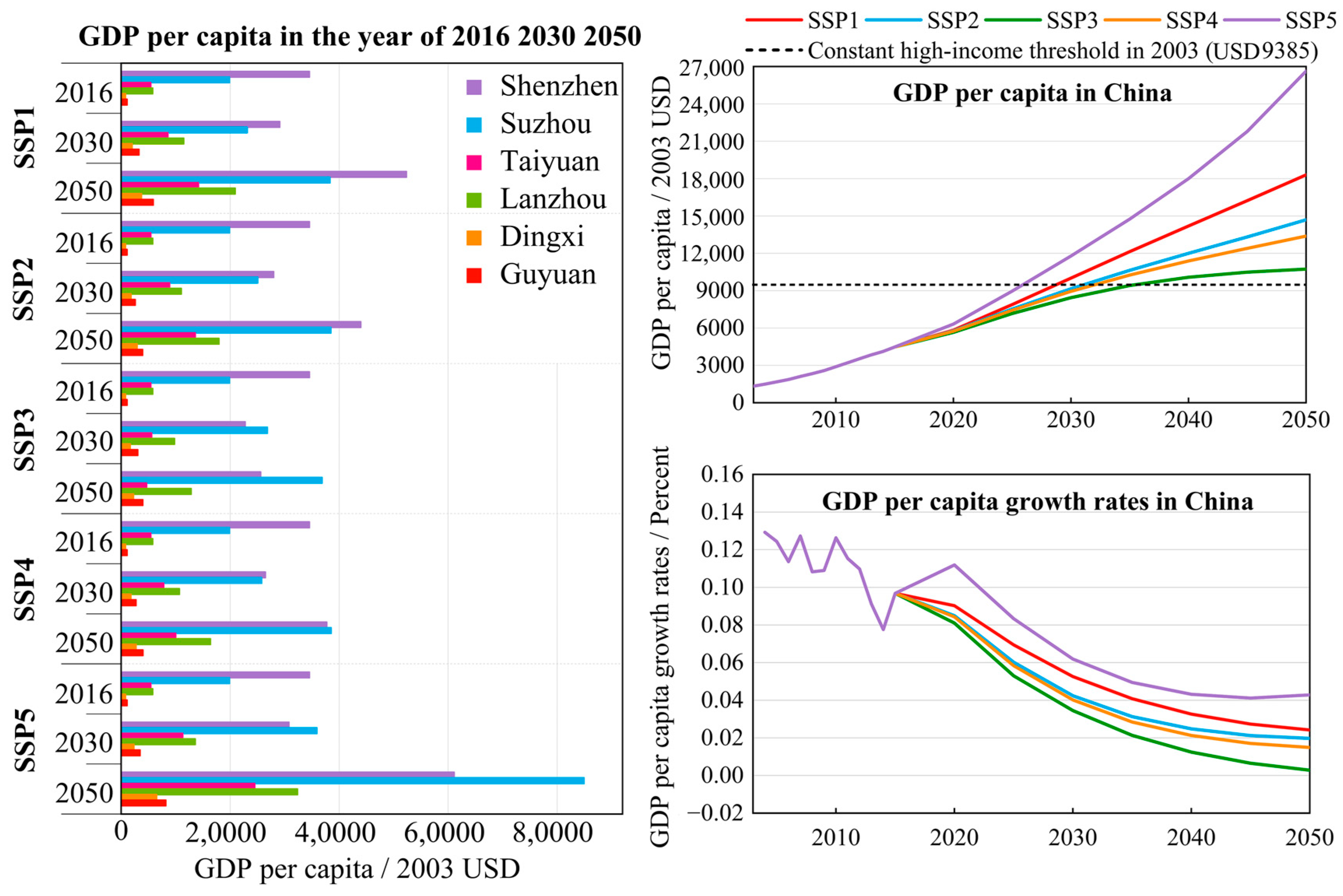
Applying the World Bank’s criteria for per capita income in 2016, based on the regional GDP and population at the end of that year, 342 prefecture-level cities are divided into high-, upper-middle-, lower-middle- and low-income regions. Shenzhen and Suzhou were selected as representative high-income areas, Taiyuan and Lanzhou as representative middle-income areas, Dingxi and Guyuan as representative low-income areas (Table 4), and four cities of Anhui Province were selected as additional representatives. The statistical data after conversion are compared with the projection results of the economic model in the same period (Figure 1), and the fitting effect is good.
Table 4.
Basic statistics for representative prefecture-level cities in 2016.
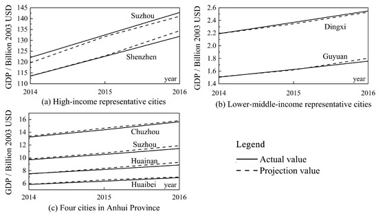
Figure 1.
Comparison of economic projection errors between the representative cities and four cities in Anhui Province.
3.2. Population Projection for Prefecture-Level Cities in China
In the SSPs, the absolute value of China’s total population shows a trend of first increasing and then decreasing, with the turning point in approximately 2035. In 2010, the population of China was approximately 1.333 billion. In the SSP2 scenario, the population increases to 1.458 billion by 2030, reaches a peak of 1.460 billion five years later, and then gradually decreases to 1.380 billion by 2050. The projected data are close to those of the Population Division of the United Nations Department of Economic and Social Affairs, which projects that the population of China will rise to 1.441 billion in 2030 and fall to 1.365 billion in 2050.
By 2050, the overall development of the population in China’s regions in the SSPs has the following three characteristics. (1) Generally, the population is still delineated by the Hu Huanyong line, showing a pattern of a greater population in the east than in the west. (2) With the North China Plain and Sichuan Basin as population concentration centers, the population gradually decreases from the inside to the outside. (3) Large developed cities, such as Shanghai and Guangzhou, still maintain a large population.
As shown in Figure 2, in 2050, the areas with a population of 10 million in the five SSPs have both massive and scattered distributions. The massive distributions are mainly centered on the North China Plain, including Hebei (Baoding, Shijiazhuang, Handan), Henan (Nanyang, Zhoukou, Zhengzhou), Beijing, and Tianjin; centered on the Sichuan Basin, including Chengdu and Chongqing; and Suzhou and Shanghai in the middle and lower reaches of the Yangtze River Plain. The scattered areas are Harbin, Wuhan, Guangzhou, Shenzhen, and other places in the northeast. Among the municipalities directly under the central government, Chongqing and Shanghai maintain a total population of more than 20 million under each path, Beijing has a total population of approximately 18–19 million, and Tianjin has the smallest population, with no more than 12 million. In the five pathways, the areas with a population below 300 thousand are mainly distributed in the Qinghai–Tibet region, including the Linzhi and Ali regions in Tibet, Golog Tibetan Autonomous Prefecture in Qinghai, and Jiayuguan in Gansu. The populations of Haibei Tibetan Autonomous Prefecture and Huangnan Tibetan Autonomous Prefecture are below 300 thousand in SSP3 and SSP4 and just over 300 thousand in SSP1 and SSP5.
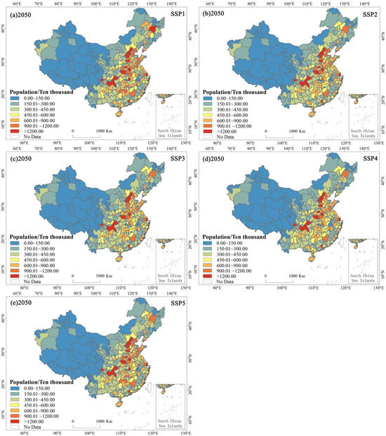
Figure 2.
Population distribution of prefecture-level cities in the SSPs in 2050.
The population growth rates of Zhangjiakou in SSP2 and Chengde, Qinhuangdao, Tangshan, and Zhangjiakou in SSP3 and SSP4 are less than 20% in 2050, while the population growth rates of Hebei and Henan are more than 20% in all pathways. The population growth rates of Hubei and Hunan in 2050 are positive in all five pathways, but under the same path, the population growth rate of Hunan is higher than that of Hubei. For example, in SSP1, except for Changde, the population of Hunan in 2050 increases by nearly 30% compared with the 2010 population. In some areas, such as Chenzhou and Changsha, the growth rate is more than 30%, while in SSP1, the population growth rate of Hubei is approximately 20% and not more than 30%. Compared with the 2010 population, the population of Haikou and Sanya in 2050 reflects 30% growth. However, the population growth rate in the same path in the county administrative divisions directly under the central government of Hainan is lower than that in Haikou and Sanya. While the population growth rate in SSP1 and SSP5 is more than 30% greater than that in 2010, the growth rate in SSP2 and SSP4 is 20%~25%, and the population growth rate in SSP3 is the lowest at 19%. For all five pathways, in all regions of Qinghai, Guizhou, Shanxi, Jiangxi and Guangxi; most regions of Shandong, Jiangsu, Anhui, Guangdong and Shaanxi; Wuzhong, Guyuan, and Zhongwei in Ningxia; Baiyin, Tianshui, Linxia, and Gannan in Gansu; Ganzi Tibetan Autonomous Prefecture in Sichuan; Aksu, Kizilsu Kirghiz Autonomous Prefecture, Kashi, and Hotan in Xinjiang; and Naqu, Ali, and Lin in Tibet, the population scale of the area in 2010 is basically maintained or the population slightly increases. In general, there are three regions with declining population in China: the Sichuan-Chongqing region, Zhejiang Province, and Liaoning Province. The populations of these three areas in 2050 are less than those in 2010, and the populations are shrinking.
The time point for the population decline in most areas of the country is approximately 2035, but the timing of the population decline is different for different pathways. In SSP1 and SSP5, the population in most regions begins to decline later, followed by a decline in SSP2. In SSP3, the population begins to decline the earliest in China and in the most widely involved regions, while the timing in SSP4 falls between that in SSP2 and SSP3.
The Zhejiang and Sichuan Provinces are the first regions to enter the period of population decline. Quzhou, in Zhejiang Province, is the first to enter the period of population decline in all pathways, starting in approximately 2020; Lishui and Zhoushan enter the period of population decline in 2020 in SSP2, SSP3, and SSP4; and Shaoxing, Huzhou, and Taizhou, in Zhejiang Province, enter the period of population decline in 2025 in all five pathways. For Sichuan, under SSP2, SSP3, and SSP4, Ziyang, Zigong, Deyang, Leshan, Meishan, Luzhou, Mianyang, Suining, Neijiang, and Nanchong begin to experience population decline in approximately 2025; Ziyang, Zigong, Deyang, Leshan, and Meishan also enter a period of population decline in 2025 in SSP1 and SSP5. In addition, in SSP3 and SSP4, Changji, Karamay, Hami, and Tacheng in Xinjiang are the areas with the earliest population decline, which occurs in approximately 2025. By 2050, the areas without population decline are concentrated in Henan, Hebei, and Hainan. In SSP1 and SSP5, the areas without population decline are the Bijie area in Guizhou and most areas in Hunan; under SSP3 and SSP4, population decline occurs in Hunan but later than in most areas in the country, starting in approximately 2050. Another area of concern is Qinghai, which enters a period of negative population growth after 2045 in all pathways.
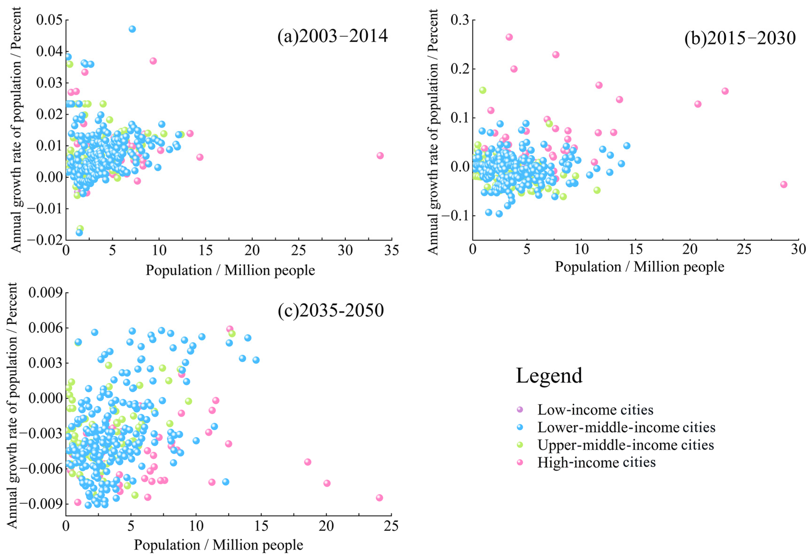
In SSP2, the average annual growth rate of the population in areas with different income levels is also clearly different in different time periods, as shown in Figure 3. Before 2015, the average annual growth rate of the population in areas with different income levels was concentrated between 0% and 2%, and a few areas showed negative population growth. The distribution of the growth rates in lower-middle-income areas is relatively concentrated, with little difference between areas. Megacities with large populations are high-income areas, with populations of approximately 33 million in 2014 and average annual population growth rates of approximately 0.5%. From 2015 to 2030, the distribution of the average annual growth rate of the population is relatively scattered but mainly falls between −5% and 5%. Most areas have negative population growth, including lower-middle-income areas and upper-middle-income areas, while the average annual growth rate of high-income areas still indicates high positive growth, except for some cities such as Yangzhou and Nantong. The megacities have populations of approximately 29 million in 2030, a decrease of nearly 4 million compared with 2014. The average annual population growth rate in this period is approximately −5%. Additionally, there are two high-income cities (Shanghai and Beijing) with rapid population growth rates of more than 10%, and by 2030, the total population of these two cities will exceed 20 million. From 2035 to 2050, the distribution of the average growth rates of the population is the most scattered. Most areas show negative population growth, and high-income areas have the most typical growth rates. Population growth rates in this period are mainly between −0.9% and −0.3%. In 2050, the total population of megacities decreases to less than 25 million. In the last stage, the total population of the two cities with rapid growth decreases to less than 20 million.
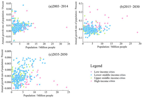
Figure 3.
Population growth rates of prefecture-level cities in China.
3.3. GDP Projection for Prefecture-Level Cities in China
In this paper, the total GDP and growth rates of 342 prefecture-level cities in China in 2030 and 2050 are analyzed for the SSPs. As shown in Figure 4, in the five SSPs, the spatial distribution pattern of GDP shows the characteristics of “high in the east and low in the west, high in the south and low in the north”. In SSP1–SSP5, the total GDP of Shanghai always remains the highest. In SSP1, the total GDP of Shanghai in 2030 will have increased by approximately 1.5 times compared with that in 2016, and by 2050 it will increase by nearly 3.5 times. In 2016, the top 10 cities in terms of GDP were Shanghai, Tianjin, Guangzhou, Beijing, Suzhou, Chongqing, Shenzhen, Chengdu, Wuxi, and Hangzhou. Changchun, Nanjing, Wuhan, and Qingdao are among the top 10 cities in the different periods and pathways. It is worth mentioning that in the development process, by 2030 and 2050, Chongqing’s GDP ranking improves rapidly. In SSP1, SSP2, and SSP4, Chongqing’s GDP ranking is upgraded from 6th to 3rd; in SSP3, Chongqing’s GDP ranking is upgraded to 2nd; and in SSP5, Chongqing’s GDP ranking improves more slowly, but its economic aggregate ranking is 4th in China. In the whole development process, Xinjiang, Qinghai, and other western provinces consistently remain at a low level of development.
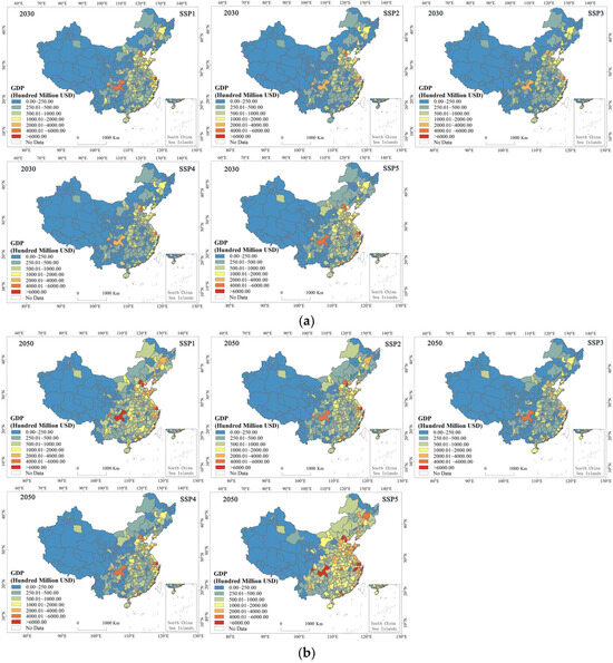
Figure 4.
GDP distributions in 2030 and 2050 in the SSPs. (a) GDP distributions in 2030. (b) GDP distributions in 2050.
The GDP projection results for prefecture-level cities in China are shown in Table 5 and Figure 5 (right). From the perspective of the GDP growth trend, the total GDP of all regions in China maintains a rapid growth rate in the SSP5 path, and the growth rate is always higher than those in the other four pathways. In contrast, SSP3 has the slowest growth rate, and it is always lower than those in the other four pathways; the growth rate in SSP1 is higher than that in SSP2, and the differences become more significant over time. The GDP growth in SSP4 is always between those in SSP2 and SSP3. From the perspective of GDP growth, the average annual growth rate of China’s GDP from 2003 to 2010 was 13%, and it has slowed since 2011. In the five SSPs, the growth rate can be maintained above 6% before 2020, and the slowdown after 2020 varies for each path. From 2041 to 2050, the annual growth rate of GDP in SSP1 is approximately 2%, which in SSP2 decreases to approximately 1.4%. The difference between SSP4 and SSP2 is small, approximately 1.0%. In SSP5, the growth rate is significantly higher than that in the other four pathways, maintaining a value of approximately 3.4% per year. In SSP3, a negative growth rate appears for the first time in 2044 and that in 2041–2050 is approximately −0.2%. On the whole, the changes in the medium- and long-term growth trends of China’s economy for the five pathways are similar to the results of Jiang et al. [20] and Leimbach et al. [4].
Table 5.
Average annual growth rate of GDP at different stages under the five SSPs.
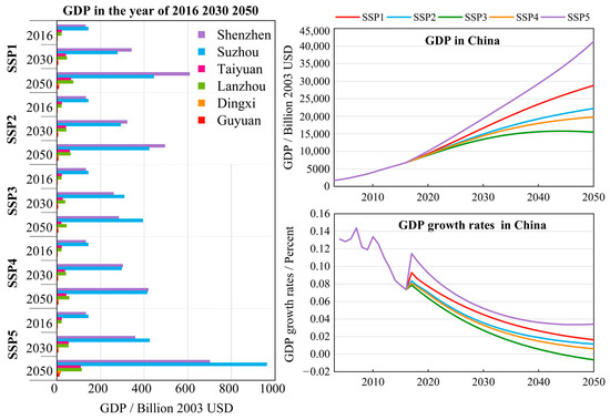
Figure 5.
Changes in total GDP of cities with different income levels, total GDP, and growth in China under SSPs.
Figure 5 (left) shows the total change in GDP in representative cities with different per capita income levels under the SSPs. Shenzhen and Suzhou, which represent high GDP per capita income cities, maintain their total GDP in the top 10 in China under the five SSPs. In 2016, the total GDP change in Suzhou was approximately USD 142.8 billion, slightly higher than that in Shenzhen, which was approximately USD 131.8 billion. Under SSP3 and SSP5, the total GDP of Suzhou is always ahead of that of Shenzhen, while under SSP1, SSP2, and SSP4, GDP in Shenzhen surpasses that of Suzhou. Under the SSPs, the total GDP of Taiyuan and Lanzhou, the representative upper-middle-income cities, fluctuates in the range of 90–130, while the total GDP change in these cities in 2016 was approximately USD 20 billion. By 2050, under SSP1, the total GDP change in Taiyuan will increase to USD 63.5 billion, while that in Lanzhou will be USD 73.6 billion, nearly 2 times and 2.7 times higher than that in 2016, respectively. Under the rapid development of SSP5, the total GDP change in Taiyuan and Lanzhou increases to USD 107.8 billion and USD 112.5 billion, approximately 4 and 4.5 times higher than that in 2016, respectively. In the lower-middle-income representatives Dingxi and Guyuan, total GDP is maintained at 300–320 under the SSPs. In 2016, the total GDP change in Dingxi city was USD 2.5 billion and that in Guyuan city was USD 1.8 billion. Under the current SSP2 development path, the cities of Dingxi and Guyuan achieve a USD 7.5 billion and USD 5.2 billion GDP change, respectively, in 2050, a nearly two-fold increase.
3.4. Per Capita Income Projection for Prefecture-Level Cities in China
The projection of per capita GDP levels of prefecture-level cities in China is determined by the projection results for population and GDP. The projection results for the per capita GDP of prefecture-level cities in China in 2030 and 2050 are selected for analysis. The distributions of the per capita GDP levels under the SSPs are shown in Figure 6. The areas with high per capita income are mainly distributed in those eastern areas with high economic development levels and northwestern areas with medium economic levels but relatively small populations. In 2015, the top 10 cities in terms of GDP per capita were Ordos, Karamay, Dongying, Shenzhen, Guangzhou, Suzhou, Baotou, Wuxi, Zhuhai, and Nanjing. According to the long-term per capita income levels projected by the SSPs, Karamay, Dongying, Shenzhen, and Baotou will remain at the forefront of China in this ranking.
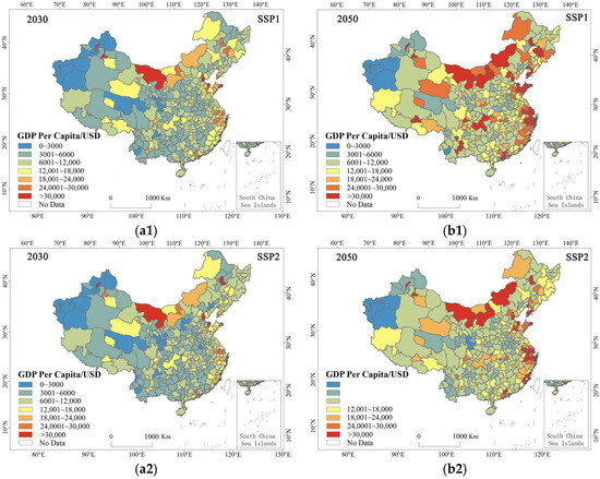
Figure 6.
Total distributions of per capita GDP in 2030 and 2050 under the SSPs. (a1) Total distributions of per capita GDP in 2030 under the SSP1. (b1) Total distributions of per capita GDP in 2050 under the SSP1. (a2) Total distributions of per capita GDP in 2030 under the SSP2. (b2) Total distributions of per capita GDP in 2050 under the SSP2. (a3) Total distributions of per capita GDP in 2030 under the SSP3. (b3) Total distributions of per capita GDP in 2050 under the SSP3. (a4) Total distributions of per capita GDP in 2030 under the SSP4. (b4) Total distributions of per capita GDP in 2050 under the SSP4. (a5) Total distributions of per capita GDP in 2030 under the SSP5. (b5) Total distributions of per capita GDP in 2050 under the SSP5.
The total GDP per capita and growth in the SSPs are shown in Figure 7 (right) and Table 6. The dotted line in Figure 7 represents the high-income threshold in 2003 (because the World Bank updates the income threshold only considering annual inflation, the threshold is set as a constant in this paper for comparison with the GDP projection in constant 2003 US dollars) [43,44]. From the perspective of the changes in the absolute values of per capita GDP, the change characteristics of per capita GDP under different SSPs are consistent with the changes in total GDP. SSP5 will first exceed the high-income threshold in approximately 2025 and SSP1 will exceed it later, in approximately 2028. Although the time point for crossing the threshold is slightly later, SSP2 and SSP4 will also significantly surpass the high-income threshold in approximately 2031 and 2032, respectively. However, SSP3 struggles, with growth stagnating in approximately 2040, making it difficult to truly eliminate the middle-income trap, although SSP3 exceeds the threshold in approximately 2037. Although the per capita GDP growth rate of all pathways generally showed a slowing trend, the degree of decline was different. The growth rates of SSP1, SSP2 and SSP4 dropped from 12% in 2005 to 3.3%, 2.5%, and 2.1% in 2040, respectively, and then slowed further in the following decade to 2.4%, 2%, and 1.5% in 2050. The growth rate of SSP3 shows a more obvious decline in the later period, with the growth rate dropping to only 0.3% in 2050. Under SSP5, the growth rate is always higher than that in the other four pathways, and it increases from 9.7% in 2015 to 11.2% in 2020, then begins to decline, ultimately being maintained at 4.3% in 2050.
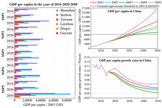
Figure 7.
Changes in total GDP per capita of cities at different income levels (left), total GDP per capita, and growth rates (right) in China under the SSPs.
Table 6.
Average annual growth rate of GDP per capita at different stages under the five SSPs.
The levels of GDP per capita for different income levels under different pathways are also compared, as shown in Figure 7 (left). Shenzhen and Suzhou, as representatives of the high-income cities, have a total population of more than 11 million people in the five pathways, but due to their high level of economic development, their per capita GDP also maintains a high advantage in the five SSPs. Under the SSPs in 2020, the growth rate of GDP per capita in these two cities decreases, first significantly and then slowly, mainly because the population growth rates of the two cities reach their peaks in 2020, affecting the per capita GDP levels. Shenzhen’s GDP per capita under SSP1 and SSP2 is higher than that of Suzhou, while Suzhou’s GDP under the other three pathways is higher than that of Shenzhen. Under SSP1, the per capita GDP of Shenzhen will reach USD 52,300 in 2050 and that of Suzhou will reach USD 38,300 in the same period. Under SSP2, which maintains the current development situation, in 2015, Suzhou’s per capita GDP was USD 19,900, and it is projected to increase to USD 38,500 by 2050, but there is still a gap between it and Shenzhen’s USD 44,000 in that same year. Under the rapid development of SSP5, Suzhou’s per capita GDP will increase almost threefold to USD 84,900 by 2050, which is nearly 0.3 times higher than Shenzhen’s in the same period. Due to the small differences in population and economic development between Taiyuan and Lanzhou, the representative upper-middle-income cities, the differences in per capita GDP levels between the two cities are small for the different pathways. As a whole, due to the relatively small population advantage, the per capita GDP of Lanzhou is larger than that of Taiyuan in the five pathways. Under SSP1, Lanzhou grows from USD 5800 in 2015 to USD 20,900 in 2050, which is higher than the growth to USD 14,100 in Taiyuan in the same period. Under the rapid development of SSP5, the per capita GDP of Lanzhou will increase to USD 32,300 by 2050, an increase of approximately 3.5 times compared with that in 2015. It is projected that the per capita GDP of Taiyuan will increase to USD 24,500 in the same period, an increase of nearly 2.5 times that in 2015. Dingxi and Guyuan represent lower-middle-income cities, and their per capita GDP increases to different degrees in the five SSPs. The situation of per capita GDP in Guyuan is similar to that in Dingxi. Under the current development of SSP2, Dingxi’s per capita GDP increases from USD 800 in 2015 to USD 2900 in 2050, an increase of nearly 1.7 times, nearly doubling the per capita GDP growth rate (2.7 times) under SSP1 in the same period and much lower than the per capita GDP level of USD 6500 under SSP5.
3.5. Spatial Distribution of Land Use and Efficiency
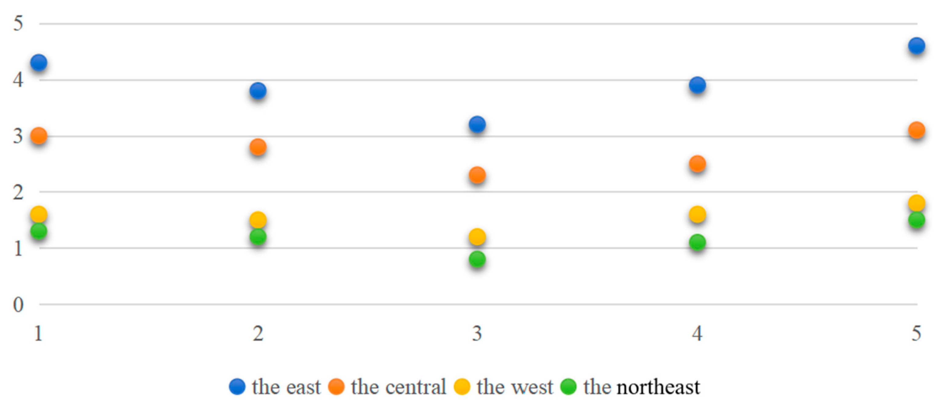
Research shows that in 2050 (Figure 8), the expansion rate of land use in the eastern region under the SSP5 pathway reaches an average annual rate of 4.6%, significantly higher than the 3.2% in SSP3, while the land use expansion in Northeast China has always maintained a low level of no more than 1.5%. Generally speaking, expansion rate of land use under the SSPs in China presents a gradient decreasing pattern in the order of east, middle, west, and northeast.
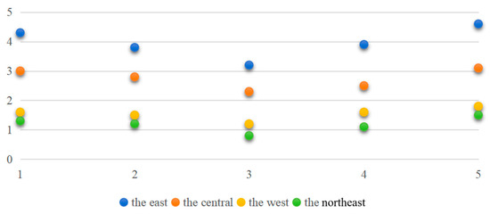
Figure 8.
The expansion rate of land use in four regions of China in 2050 under the SSPs.
Research reveals a significant increase in land productivity through the SSP1 pathway; the GDP per unit of construction land will reach 123,000 yuan/hectare by 2050, which is 38% higher than SSP5. However, SSP3 exhibits a “double low” characteristic—a 12% decrease in land development intensity and only a 0.3% increase in utilization efficiency.
4. Discussion
Based on the SSP scenarios, this paper simulated the changes in population and GDP of Chinese prefecture-level cities by 2050 and then projected the trend in income level change, which provides an intuitive and reliable basis for determining the timing and identifying the development pattern with which China is able to cross the middle-income trap. The results showed that SSP5, SSP1, SSP2, and SSP4 will cross the high-income threshold in approximately 2025, 2028, 2031, and 2032, respectively; although SSP3 exceeds the threshold in approximately 2037, growth then begins to stagnate, and it is likely that SSP3 will not ultimately escape the middle-income trap. In 2050, the growth rate of per capita GDP is projected to remain in a range between 0.3% (SSP3) and 4.3% (SSP5). By 2050, China’s population is expected to first increase and then decrease under the five pathways (peak in 2035), and China’s GDP growth rates generally show a trend of slowing down.
Thanks to China’s absolute size and its unusual openness for a continental economy, it seems unlikely that it will fall into the middle-income trap (except under SSP3). SSP1 and SSP5 are probably the more sensible and efficient development pathways, but SSP2 and SSP4 also seem to be acceptable. However, China should be alert to the growing domestic friction caused by regional income disparities, urban congestion, environmental strain, and corruption in the process of sustained economic growth; trouble at home, rather than abroad, could bring down the awakened giant. In particular, SSP2, with its continuing societal stratification, limited social cohesion, and slow improvement in income inequality, and SSP4, with its high inequality, feel uncertain and unreliable in a changing and uncertain future. In fact, disturbing signs have been found in the spatial projections of prefecture-level cities in this paper. Under the five paths, it is still difficult to break across the Hu Huanyong line in terms of the total population distribution in various regions in 2050. There is no discernible shift in population from large developed cities to small ones. Although the range of high-income areas is expanding, the level of per capita income in different regions still varies significantly. If managed badly, spatial and social problems may lead to the waste of the economic benefits of scale economies through congestion, pollution, social discord, and corruption, sharply reducing the resources available for investment and growth. If they are well managed, these social and spatial trends may, in turn, feed back into improved scale economies through the agglomeration of production and incentives for more rapid skill formation [45].
SSP5 crosses the high-income threshold earlier than SSP1. An important reason for this is setting a high investment level for SSP5 in the parameter setting. However, the historical development experience of developed countries such as the United States, Japan, and South Korea tells us that such high-intensity investment is difficult to maintain for a long period of time [46]. Moreover, in the SSP storylines, SSP1 has a somewhat less rapid economic growth than SSP5 but is compensated by other factors, such as better environmental quality and a higher level of equity [47]. These characteristics are not reflected in the results of this paper because the basic neoclassical economic model cannot take the environment, governance capacity, and other factors into account. Indeed, the neoclassical models, in their simplest form, are still the prevalent tools for exploring historic and future economic growth paths [4]. However, neoclassical growth theories are being challenged by endogenous growth theories, which are stimulating a new generation of research into economic growth [31,48]. Building an endogenous model of sustained economic growth considering energy depletion, pollution control, and knowledge accumulation and developing a more scientific and convincing extended GDP scenario may be a direction for future research.
The study also found significant path dependence in the response of land systems. Firstly, the rapid urbanization of SSP5 has led to an average annual expansion of 3.2% in land use but is accompanied by an 18% reduction in arable land and fragmentation of ecological spaces. Secondly, SSP1 achieves intensive land use through technological innovation, reducing land consumption per unit of GDP by 42%. Finally, the phenomenon of “inefficient expansion” has emerged in western cities under SSP4, with a land development elasticity coefficient of 1.5, exacerbating the contradiction between people and land. These findings confirm Leimbach et al.’s argument that uneven regional development exacerbates land pressure, and provide empirical support for Dong et al.’s multi-scenario land use model [9]. It is suggested that differentiated land management policies should be established; the eastern part should focus on stock optimization, and the western part should explore the “ecological-economic” collaborative model. Follow-up research can integrate the evaluation model of ecosystem services and deepen the analysis of land versatility.
The findings of this study on land system dynamics under different SSP scenarios align with and complement international research on urbanization, land use efficiency, and regional disparities. With regard to urbanization and land expansion under SSP5, this study highlights that SSP5 (fossil-fueled development) leads to a 3.2% annual expansion in land use, accompanied by an 18% reduction in arable land and ecological fragmentation. This mirrors global trends. In Uruguay, soybean cultivation increased by 1000%, causing grassland degradation and soil erosion, similar to the ecological costs of SSP5’s rapid urbanization. Yantai City faced similar issues of inefficient land use during urbanization, necessitating stricter farmland protection policies. SSP4 (unequal pathway) results in inefficient expansion in western cities, with a land development elasticity coefficient of 1.5, reflecting global regional disparities. Low- and middle-income countries exhibit lower PBUA (per capita built-up area) than high-income countries, with Africa and Asia facing policy coordination challenges [49].
5. Conclusions
This study evaluates the spatial–temporal evolution of land use intensity and regional development under five shared socioeconomic pathways (SSPs) through prefecture-level projections in China (2020–2050). This study uses a variety of methods to predict the population, GDP, and land use in China in turn. The theoretical and practical significance of this study is as follows:
- (1)
- SSP5 (conventional development) and SSP1 (sustainability) achieve high-income thresholds by 2025/2028 with intensive land development, while SSP3 (fragmentation) risks stagnation post-2037 accompanied by inefficient land use.
- (2)
- Spatial analysis identifies persistent dualism across the Hu Huanyong Line—83.6% of urban land expansion concentrates in eastern regions, whereas western areas exhibit 56% lower land productivity.
- (3)
- By 2050, regional land use efficiency differentials (0.3–4.3% Gross Domestic Product/capita growth) highlight challenges in balancing urban agglomeration and ecological conservation.
These findings provide empirical evidence for optimizing land allocation policies during China’s economic transition.
Author Contributions
Conceptualization, X.Z. and F.Z.; methodology, M.Y.; formal analysis, Y.L.; resources, R.G.; data curation, Y.L.; writing—original draft preparation, X.Z.; writing—review and editing, F.Z.; supervision, F.Z. All authors have read and agreed to the published version of the manuscript.
Funding
This work was supported by the Science and Technology Project of Information and Communication Company of Gansu Power Company, State Grid of China (Project No. 52272323000C).
Data Availability Statement
The original contributions presented in this study are included in the article. Further inquiries can be directed to the corresponding author.
Conflicts of Interest
Authors X.Z., M.Y. and R.G. were employed by the Information and Communication Company of Gansu Power Company. The remaining authors declare that the research was conducted in the absence of any commercial or financial relationships that could be construed as potential conflicts of interest.
References
- O’Neill, B.; Kriegler, E.; Riahi, K.; Ebi, K.; Hallegatte, S.; Carter, T.; Mathur, R.; van Vuuren, D. A new scenario framework for climate change research: The concept of shared socioeconomic pathways. Clim. Change 2014, 122, 387–400. [Google Scholar] [CrossRef]
- Van Vuuren, D.; Kriegler, E.; O’Neill, B.; Ebi, K.; Riahi, K.; Carter, T.; Edmonds, J.; Hallegatte, S.; Kram, T.; Mathur, R.; et al. A new scenario framework for Climate Change Research: Scenario matrix architecture. Clim. Change 2014, 122, 373–386. [Google Scholar] [CrossRef]
- Dellink, R.; Chateau, J.; Lanzi, E.; Magné, B. Long-term economic growth projections in the Shared Socioeconomic Pathways. Glob. Environ. Change Hum. Policy Dimens. 2017, 42, 200–214. [Google Scholar] [CrossRef]
- Leimbach, M.; Kriegler, E.; Roming, N.; Schwanitz, J. Future growth patterns of world regions—A GDP scenario approach. Glob. Environ. Change Hum. Policy Dimens. 2017, 42, 215–225. [Google Scholar] [CrossRef]
- Jiang, T.; Zhao, J.; Cao, L.; Wang, Y.; Su, B.; Jing, C.; Wang, R.; Gao, C. Projection of national and provincial economy under the shared socioeconomic pathways in China. Clim. Change Res. 2018, 14, 50–58. [Google Scholar] [CrossRef]
- Guo, A.; Ding, X.; Zhong, F.; Cheng, Q.; Huang, C. Predicting the Future Chinese Population using Shared Socioeconomic Pathways, the Sixth National Population Census, and a PDE Model. Sustainability 2019, 11, 3686. [Google Scholar] [CrossRef]
- Wang, D.; Luo, H.; Grunder, O.; Lin, Y.; Guo, H. Multi-step ahead electricity price forecasting using a hybrid model based on two-layer decomposition technique and BP neural network optimized by firefly algorithm. Appl. Energy 2017, 190, 390–407. [Google Scholar] [CrossRef]
- Ding, X.; Zhong, F.; Mao, J.; Song, X.; Huang, C. Provincial urbanization projected to 2050 under the shared socioeconomic pathways in China. Adv. Clim. Change Res. 2018, 14, 392. [Google Scholar] [CrossRef]
- Dong, N.; You, L.; Cai, W.; Li, G.; Lin, H. Land use projections in China under global socioeconomic and emission scenarios: Utilizing a scenario-based land-use change assessment framework. Glob. Environ. Change-Hum. Policy Dimens. 2018, 50, 164–177. [Google Scholar] [CrossRef]
- Glawe, L.; Wagner, H. China in the middle-income trap? China Econ. Rev. 2020, 60, S1043951X19300033. [Google Scholar] [CrossRef]
- Yao, Y. Chapter 7—The Chinese Growth Miracle. In Handbook of Economic Growth; Aghion, P., Durlauf, S.N., Eds.; Elsevier: Amsterdam, The Netherlands, 2014; Volume 2, pp. 943–1031. [Google Scholar]
- Woo, W. China Meets the Middle-Income Trap: The Large Potholes in the Road to Catching-Up. J. Chin. Econ. Bus. Stud. 2012, 10, 313–336. [Google Scholar] [CrossRef]
- Cai, F. Is There a ’Middle-Income Trap’? Theories, Experiences and Relevance to China. China World Econ. 2012, 20, 49–61. [Google Scholar] [CrossRef]
- Felipe, J.; Abdon, A.; Kumar, U. Tracking the Middle-Income Trap: What is it, Who is in it, and Why? In ERN: Consumption; Saving (Consumption) (Topic); Levy Economics Institute: Annandale-on-Hudson, NY, USA, 2012. [Google Scholar]
- Barro, R.; Sala-i-Martin, X. Economic Growth, 2nd ed.; MIT Press: Cambridge, MA, USA, 2003. [Google Scholar]
- Li, Z.; Zhou, C.; Yang, X.; Chen, X.; Meng, F.; Lu, C.; Pan, T.; Qi, W. Urban landscape extraction and analysis in the mega-city of China’s coastal regions using high-resolution satellite imagery: A case of Shanghai, China. Int. J. Appl. Earth Obs. Geoinf. 2018, 72, 140–150. [Google Scholar] [CrossRef]
- Jiang, T.; Wang, Y.; Yuan, J.; Chen, Y.; Gao, X.; Jing, C.; Wang, G.; Wu, X.; Zhao, C. Projection of population and economy in the Belt and Road countries (2020–2060). Clim. Change Res. 2018, 14, 155–164. [Google Scholar] [CrossRef]
- Zhou, J.; Jiang, T.; Wang, Y.; Su, B.; Tao, H.; Qin, J.; Zhai, J. Spatiotemporal variations of aridity index over the Belt and Road region under the 1.5 °C and 2.0 °C warming scenarios. J. Geogr. Sci. 2020, 30, 37–52. [Google Scholar] [CrossRef]
- Huang, J.; Qin, D.; Jiang, T.; Wang, Y.; Feng, Z.; Zhai, J.; Cao, L.; Chao, Q.; Xu, X.; Wang, G.; et al. Effect of Fertility Policy Changes on the Population Structure and Economy of China: From the Perspective of the Shared Socioeconomic Pathways. Earths Future 2019, 7, 250–265. [Google Scholar] [CrossRef]
- Jiang, T.; Zhao, J.; Jing, C.; Cao, L.; Wang, Y.; Sun, H.; Wang, A.; Huang, J.; Su, B.; Wang, R. National and Provincial Population Projected to 2100 Under the Shared Socioeconomic Pathways in China. Clim. Change Res. 2017, 13, 128. [Google Scholar] [CrossRef]
- Yao, S.; Li, Y.; Jiang, H.; Wang, X.; Ran, Q.; Ding, X.; Wang, H.; Ding, A. Predicting Land Use Changes under Shared Socioeconomic Pathway–Representative Concentration Pathway Scenarios to Support Sustainable Planning in High-Density Urban Areas: A Case Study of Hangzhou, Southeastern China. Buildings 2024, 14, 2165. [Google Scholar] [CrossRef]
- Wang, Z.; Li, X.; Mao, Y.; Li, L.; Wang, X.; Lin, Q. Dynamic simulation of land use change and assessment of carbon storage based on climate change scenarios at the city level: A case study of Bortala, China. Ecol. Indic. 2022, 134, 108499. [Google Scholar] [CrossRef]
- Lutz, W. Population, Development, Environment: Understanding Their Interactions in Mauritius; Springer: Berlin/Heidelberg, Germany, 1994. [Google Scholar]
- Meng, L.G.; Li, C.L.; Hu, G. Predictions of China’s population structure based on the PDF model. Zhongguo Renkou Ziyuan Yu Huan Jing/China Popul. Resour. Environ. 2014, 24, 132–141. [Google Scholar] [CrossRef]
- Gallopin, G.; Raskin, P. Global Sustainability: Bending the Curve; Routledge: England, UK, 2002. [Google Scholar]
- Kemp-Benedict, E.; Heaps, C.; Raskin, P. Global Scenario Group Futures; Technical Notes; Stockholm Environmeny Institute: Stockholm, Sweden, 2002. [Google Scholar]
- Nakicenovic, N.; Alcamo, J.; Davis, G.; Vries, B.d.; Fenhann, J.V.; Gaffin, S.R.; Gregory, K.; Grubler, A.; Jung, T.Y.; Kram, T.; et al. Special Report on Emissions Scenarios: A Special Report of Working Group III of the Intergovernmental Panel on Climate Change; Cambridge University Press: Cambridge, MA, USA, 2000. [Google Scholar]
- Huang, Y.; Ruoen, R.; Liu, X. Capital stock estimates in Chinese manufacturing by perpetual inventory approach. China Econ. Q. 2002, 1, 377–396. [Google Scholar]
- Lejour, A.; Veenendaal, P.; Verweij, G.; van Leeuwen, N. Worldscan; a Model for International Economic Policy Analysis; CPB Netherlands Bureau for Economic Policy Analysis: Den Haag, The Netherlands, 2006. [Google Scholar]
- Rumelhart, D.; McClelland, J.; Group, P.R. Parallel Distributed Processing, Volume 1: Explorations in the Microstructure of Cognition: Foundations; MIT Press: Cambridge, MA, USA, 1986. [Google Scholar]
- Kemp-Benedict, E. Downscaling global income scenarios assuming institutional convergence or divergence. Glob. Environ. Change 2012, 22, 877–883. [Google Scholar] [CrossRef]
- McKibbin, W.; Pearce, D.; Stegman, A. Climate change scenarios and long term projections. Clim. Change 2009, 97, 23–47. [Google Scholar] [CrossRef]
- Mccombie, J.; Thirlwall, A. Economic Growth and the Balance-of-Payments Constraint; Macmillan London Ltd.: London, UK; Basingstoke, UK, 1993. [Google Scholar]
- Solow, R. A Contribution to the Theory of Economic Growth. Q. J. Econ. 1956, 70, 65–94. [Google Scholar] [CrossRef]
- Goldsmith, R. A Perpetual Inventory of National Wealth. In Studies in Income and Wealth; National Bureau of Economic Research, Inc.: Cambridge, MA, USA, 1951; Volume 14, pp. 5–73. [Google Scholar]
- Ke, S.; Xiang, J. Estimation of the Fixed Capital Stocks in Chinese Cities for 1996–2009. Stat. Res. 2012, 7, 19–24. [Google Scholar] [CrossRef]
- Zhang, J. Estimation of China’s provincial capital stock (1952–2004) with applications. J. Chin. Econ. Bus. Stud. 2008, 6, 177–196. [Google Scholar] [CrossRef]
- Kc, S.; Lutz, W. The human core of the shared socioeconomic pathways: Population scenarios by age, sex and level of education for all countries to 2100. Glob. Environ. Change 2017, 42, 181–192. [Google Scholar] [CrossRef]
- Guo, L.; Che, S. The Effect of China’s Labor Participation Rate and Demographic Dividend on Economic Growth. J. Cent. Univ. Financ. Econ. 2011, 9, 47–53. [Google Scholar]
- Rumelhart, D.; Hinton, G.; Williams, R. Learning representations by back-propagating errors. Nature 1986, 323, 533–536. [Google Scholar] [CrossRef]
- Johansson, Å.; Guillemette, Y.; Murtin, F.; Turner, D.; Nicoletti, G.; de la Maisonneuve, C.; Bagnoli, P.; Bousquet, G.; Spinelli, F. Long-Term Growth Scenarios; OECD Publishing: Paris, France, 2013. [Google Scholar]
- Wang, J.; Ge, Y. Population Trends in China under the Universal Two-Child Policy. Popul. Res. 2016, 40, 3–21. [Google Scholar]
- Nielsen, L. Classifications of Countries Based on Their Level of Development: How it is Done and How it Could Be Done. IMF Work. Pap. 2011, 11, 46. [Google Scholar] [CrossRef]
- Bank, T.W. World Bank Country and Lending Groups. Available online: http://data.worldbank.org/about/country-and-lending-groups (accessed on 5 November 2024).
- Gill, I.; Kharas, H. An East Asian Renaissance: Ideas for Economic Growth; The World Bank Group: Washington, DC, USA, 2007. [Google Scholar]
- Attanasio, O.; Picci, L.; Scorcu, A. Saving, investment and growth: A macroeconomic analysis with a panel of countries. Rev. Econ. Stat. 2000, 82, 182–211. [Google Scholar] [CrossRef]
- O’Neill, B.; Kriegler, E.; Ebi, K.; Kemp-Benedict, E.; Riahi, K.; Rothman, D.; van Ruijven, B.; van Vuuren, D.; Birkmann, J.; Kok, K.; et al. The roads ahead: Narratives for shared socioeconomic pathways describing world futures in the 21st century. Glob. Environ. Change 2017, 42, 169–180. [Google Scholar] [CrossRef]
- Aghion, P.; Howitt, P.; Brant-Collett, M.; García-Peñalosa, C. Endogenous Growth Theory; MIT Press: Cambridge, MA, USA, 1998. [Google Scholar]
- Seto, K.C.; Güneralp, B.; Hutyra, L.R. Global Urban Expansion and Its Implications for Land Use. Proc. Natl. Acad. Sci. USA 2012, 109, 16083–16088. [Google Scholar] [CrossRef] [PubMed]


Disclaimer/Publisher’s Note: The statements, opinions and data contained in all publications are solely those of the individual author(s) and contributor(s) and not of MDPI and/or the editor(s). MDPI and/or the editor(s) disclaim responsibility for any injury to people or property resulting from any ideas, methods, instructions or products referred to in the content. |
© 2025 by the authors. Licensee MDPI, Basel, Switzerland. This article is an open access article distributed under the terms and conditions of the Creative Commons Attribution (CC BY) license (https://creativecommons.org/licenses/by/4.0/).