Article

Nonlinear and Spatially Varying Impacts of Natural and Socioeconomic Factors on Multidimensional Human Health: A Geographically Weighted Machine Learning Approach

1
College of Geography and Remote Sensing, Hohai University, Nanjing 211100, China
2
School of Environmental and Geographical Sciences, Shanghai Normal University, Shanghai 200234, China
*
Author to whom correspondence should be addressed.
Land 2025, 14(12), 2324; https://doi.org/10.3390/land14122324
Submission received: 17 September 2025 / Revised: 20 November 2025 / Accepted: 22 November 2025 / Published: 26 November 2025

Abstract

Ensuring healthy lives is both crucial for residents’ quality of life and a core objective of the Sustainable Development Goals. While numerous studies have examined the drivers of human health, few have distinguished between average health and extreme health outcomes. Moreover, the nonlinear effects of various determinants on multidimensional human health remain underexplored. This study aims to investigate the spatially varying contributions of natural and socioeconomic factors to multidimensional human health, focusing particularly on their nonlinear relationships. We first quantified multidimensional human health at the prefectural level of China, including average health (Life Expectancy), extreme health (Longevity Index and Centenarian Index), and subjective health (Self-Rated Health). We then combined the Geographically Weighted Random Forest model with the SHAP interpretations to investigate the impacts of natural and socioeconomic factors. Through the GWRF-SHAP framework, we estimated the nonlinear relationships between the four health indicators and their key influencing factors. We found that: (1) The four health indicators exhibited significant positive correlations, except for the relationship between Centenarian Index and Self-Rated Health. (2) Extreme health outcomes (Longevity and Centenarian Index) were predominantly influenced by natural factors, whereas average and subjective health (Life Expectancy and Self-Rated Health) were more strongly associated with socioeconomic conditions. (3) The dominant determinants of human health varied across regions, but socioeconomic factors generally showed stronger influences in northwestern China. (4) Both socioeconomic and natural factors exhibited nonlinear effects and threshold behaviors on health outcomes. These findings suggest that improving socioeconomic conditions is beneficial for enhancing both average and subjective health, whereas managing the natural environment is crucial for promoting extreme levels of health. Our study advocates a multidimensional, spatially tailored, and threshold-sensitive approach to health management.

1. Introduction

Health underpins human well-being and satisfaction, serving as a foundational goal in societal development initiatives globally. The United Nations Sustainable Development Goal 3 explicitly calls for diverse strategies to ensure healthy lives and promote human welfare [1]. Human health is shaped by the interplay of intrinsic factors, such as genetic predispositions, habits, and lifestyles, as well as extrinsic factors, including natural environment and socioeconomic development [2,3,4,5]. Among these, extrinsic factors like natural and socioeconomic factors not only exert a shaping influence on intrinsic determinants but also exhibit pronounced spatial heterogeneity at the macro level and thus were the key moderating factors [6,7,8,9,10,11,12]. Previous studies have postulated that with increasing urbanization and agricultural intensification, the contribution of natural environments to human well-being tends to decline, while the influence of socioeconomic factors becomes more pronounced [6]. Therefore, a timely assessment of how natural and socioeconomic determinants jointly influence human health is essential for promoting human well-being.
Numerous studies have investigated the determinants of natural and socioeconomic factors on human health. Most of them focused on one dimension of human health [13], including life expectancy [14], longevity index [15], self-rated health level of older adults [16], heat-related mortality [17], and infant mortality [18]. However, human health is a multidimensional concept and can be generally classified into objective (e.g., life expectancy, longevity index) and subjective components (e.g., self-rated health) [19,20,21,22]. Among them, life expectancy represents the “average” health outcomes, while longevity index and premature death reflect “extreme” health outcomes [23]. These health indicators often show distinct spatial patterns [23], implying different social and ecological determinants. For instance, Wei et al. [23] found that factors like terrain were associated with longevity index, whereas life expectancy correlated more closely with air quality. Thus, to better understand the spatiotemporal pattern and determinants of human health, it is imperative to evaluate both average and extreme health outcomes.
Moreover, previous studies often investigated the determinants of human health using methods that either assume global spatial homogeneity or, while accounting for spatial heterogeneity, remain limited to capturing linear relationships. Examples include ordinary least squares regression [24], stepwise regression [25], generalized linear regression [26], hierarchical regression [27], geographically weighted regression [18], and multiscale geographically weighted regression [24]. Yet, the associations between determinants and human health are often neither spatially homogeneous nor purely linear [28]. For example, although human well-being may initially improve as environmental quality declines, further degradation beyond a certain threshold can lead to a decline in well-being [29]. Thus, overlooking spatial heterogeneity and nonlinearity in health-related factors can undermine attribution accuracy and result in biased findings [30].
Recently, the Geographically Weighted Random Forest (GWRF) model, a spatially explicit machine learning method introduced in 2019 [31], has been increasingly employed to capture spatial non-stationarity and to identify localized patterns in a wide range of applications [32]. For instance, Grekousis et al. [28] applied the GWRF approach to explore spatially varying determinants of COVID-19 mortality across the United States, revealing both locally significant predictors and complex nonlinear associations between mortality rates and associated factors. Moreover, SHapley Additive exPlanations (SHAP) has emerged as a powerful tool for improving the interpretability of machine learning models while maintaining high levels of predictive accuracy [30]. Thus, the integration of GWRF and SHAP improves health attribution by addressing nonlinearity, spatial heterogeneity, and enhancing interpretability.
This study aims to investigate the spatially varying and nonlinear impacts of natural and socioeconomic factors on multidimensional human health using the GWRF and SHAP models. Specifically, we addressed three key questions: (1) How is multidimensional human health distributed across China? (2) What are the main drivers of multidimensional human health at the global and local levels? (3) Do natural and socioeconomic factors have nonlinear effects and exhibit threshold behaviors in relation to health outcomes? To answer these questions, we first assessed multidimensional human health (Life Expectancy, Longevity Index, Centenarian Index, and Self-Rated Health) at the prefecture level in China using the latest 2020 population census data. We then used GWRF and SHAP models to reveal the spatially varying and nonlinear impacts of key determinants on multidimensional human health. Finally, we offered policy recommendations to inform health initiatives in China.

2. Materials and Methods

2.1. Data Sources

This study analyzed prefecture-level cities in China, excluding Taiwan, Hong Kong, Macao, and Xinjiang due to data limitations. Population and education data were obtained from the China Population Census Yearbook 2020. Data on income, GDP, hospital beds, medical technical personnel, air quality, and water resources were sourced from the respective provincial and municipal Statistical Yearbooks and Statistical Bulletins on Economic and Social Development. Information on roads, topography, and land use was obtained from the Resource and Environmental Science Data Platform (https://www.resdc.cn/, accessed on 30 August 2024). All other data, including temperature, precipitation, relative humidity, PM2.5, NDVI, NPP and healthcare accessibility, were retrieved from publicly available datasets [33,34,35,36,37,38,39,40,41,42,43,44,45,46]. All datasets used in this study correspond to the year 2020. Detailed information on all data sources is provided in Table A1. Administrative boundaries within China were acquired from the National Platform for Common GeoSpatial Information Services (https://www.tianditu.gov.cn/, accessed on 26 April 2024).

2.2. Quantifying Multidimensional Human Health

To comprehensively evaluate multidimensional human health, we classified health into objective and subjective components. Objective health indicators were further categorized into extreme health and average health. Extreme health was assessed using the Longevity Index and Centenarian Index (centenarians per 100,000 inhabitants) [14], while average health was gauged by Life Expectancy. Life Expectancy was calculated using the Simple Life Expectancy Table [47], and was adjusted based on the provincial life expectancy published officially.
Subjective health was measured by Self-Rated Health (percentage of the self-rated health level of the older adults), which was assessed through a single question during the Seventh Population Census of China: “Overall, how would you rate your health in the past month?” The response options included “healthy”, “basically healthy”, “unhealthy without disability”, and “unhealthy with disability”. We used the proportion of perceived “healthy” elderly to gauge Self-Rated Health. Due to the unavailability of city-level data on centenarians in Guangdong province, the 2020 provincial-level data were down-scaled to the city level based on proportional distributions derived from the 2010 census.

2.3. Selection of Influencing Factors

Based on data availability and previous studies, we built an index system of influencing factors from two key dimensions: natural factors and socioeconomic factors (Table A1). Natural environments exert multifaceted impacts on human health by supplying clean air and water, mitigating urban heat effects through climate regulation, and promoting physical activity and mental well-being through access to green and blue spaces [48,49,50]. In this study, we classified the natural factors into three key components: geographic conditions (TempAnn, HumidAnn, PrecAnn, Slope, DEM), environmental quality (AirQual, PM2.5, NPP, NDVI), and resource availability (FarmlandProp, ForestProp, GrasslandProp, WaterRespc). The geographical setting of a region—defined by its topography and climate—has been shown to exert a long-lasting and consistent influence on population health [16]. For instance, Bayentin et al. [51] identified a nonlinear association between climatic conditions and morbidity in Quebec, Canada. Robine et al. [52] also pointed out that a mild climate was beneficial for increasing life expectancy. In addition, many studies have demonstrated the impact of environmental quality on human health and well-being. For example, Liao et al. [53] found that environmental pollution tended to intensify income-related disparities in health outcomes. Moreover, previous research has demonstrated a positive association between resource availability and residents’ overall well-being [54,55]. Accordingly, the resource availability dimension was also incorporated into our analysis of the determinants of human health and well-being.
Socioeconomic factors, including human capital and built capital, improve residents’ health by providing essential services such as healthcare, technology, and financial support [56]. Numerous studies have shown that socioeconomic factors such as income, education, healthcare, and infrastructure have a positive impact on residents’ health [16,57]. For instance, Yee [56] found that in Puerto Rico, health outcomes—an essential component of human well-being—were closely linked to socioeconomic factors such as income, healthcare, and the availability of communication technologies. Thus, this study investigated potential determinants of health by focusing on five socioeconomic dimensions: education (EduYears, IllitRate), economy (Incomepc, GDPpc), population (PopDens), healthcare (MedTech, HospBeds, HospAccess), and infrastructure (RoadDens, ParkGreen).

2.4. Analyzing Influencing Factors of Human Health

2.4.1. Model Selection

We first standardized the raw data using z-score normalization and tested the collinearity of the variables using the Variance Inflation Factor (VIF) analysis. Only variables with a VIF below 10 were retained [58,59]. We finally excluded 6 variables (GDPpc, HumidAnn, PrecAnn, Slope, NPP, and FarmlandProp) and retained 17 variables for subsequent regression modeling.
To assess the necessity of accounting for spatial heterogeneity and nonlinear effects in examining the determinants of human health, we compared the performance among four models: Ordinary Least Squares (OLS), Geographically Weighted Regression (GWR), Random Forest (RF), and GWRF. Specifically, the OLS model assumes global homogeneity and linear relationships. The RF model, an ensemble learning algorithm, is capable of modeling complex nonlinear relationships without assuming a predefined form of variable interactions and has been extensively utilized in high-dimensional spatial data analysis [60]. However, the training process of RF is based on the entire sample, assuming equal weights for all observations, thereby ignoring the non-stationary characteristics inherent in geographic space [60]. In contrast, GWR introduces a spatial weighting matrix that enables model coefficients to vary with geographic location, and thus can effectively identify spatial heterogeneity [61,62]. Nevertheless, constrained by its inherent linearity assumption, GWR has a limited capacity to capture nonlinear associations and complex interactions among variables [63].
The GWRF model combines the advantages of GWR and RF by incorporating spatial heterogeneity and nonlinear variable effects within a unified modeling framework, thus improving the model’s adaptability to complex spatial processes [28]. Specifically, GWRF constructs a localized Random Forest model at each geographic location to predict the target variable at that location:
y ^ i = f ( u i , v i ) ( x i ) + ε i
where y ^ i is the predicted value at location ( u i , v i ) , x i is the corresponding feature vector, and ε i is the error term. To ensure spatial sensitivity during the model training process, GWRF constructs a spatial weight matrix W i = w i j for each observation. We used an adaptive kernel with a bi-square weighting kernel function to assign spatial weights to the observations [59,64]. The equation of the bi-square weighting kernel function is as follows [64]:
w i j = 1 ( d i j h ) 2 2 , d i j h 0 , d i j > h
where d i j represents the geographic distance between sample i and sample j , and h is the bandwidth parameter that controls the extent of the neighborhood. The optimal hyperparameters for the GWRF model were determined through grid search and ten-fold cross-validation [30,32]. The optimal values of the parameters are shown in Table A2.
To compare the performance of the models (OLS, GWR, RF, and GWRF) and select the suitable model, we introduced three evaluation metrics: the coefficient of determination ( R 2 ), the Root Mean Squared Error (RMSE), and the Mean Absolute Error (MAE). The formulas for these metrics are as follows:
R 2 = 1 i = 1 n ( y i y ^ i ) 2 i = 1 n ( y i y ¯ ) 2
R M S E = 1 n i = 1 n ( y i y ^ i ) 2
M A E = 1 n i = 1 n y i y ^ i
where n represents the total number of samples, y i is the actual observed value for the i t h sample, and y ^ i is the corresponding predicted value.
We also used the out-of-bag (OOB) root mean square error (RMSE) as an additional metric to evaluate the predictive accuracy of the GWRF model [59,64,65]. In the GWRF model, each decision tree is trained on a bootstrap sample containing approximately two-thirds of the total observations, with the remaining one-third forming the OOB set. This approach effectively simulates a cross-validation process and provides an unbiased internal estimate of model performance [32,65].

2.4.2. Model Interpretation with SHAP

Although the GWRF model performs well in prediction, its results are difficult to interpret due to its black-box characteristics. Therefore, we incorporated the SHAP framework to further analyze the GWRF model outputs [66,67]. SHAP is based on the SHapley value principle from cooperative game theory and decomposes model predictions into additive contributions from each feature [68]:
y ^ = φ 0 + m = 1 M φ m z m
where y ^ is the model output, M is the number of input features, φ 0 is the mean prediction for all samples (base value), and φ m represents the marginal contribution of the m t h feature to the prediction, z m 0 ,   1 indicates whether the feature is included in the model. The Shapley value for each feature can be expressed as [68]:
φ m = S N \ { m } S ! ( M S 1 ) ! M ! f ( S { m } ) f ( S )
where m N denotes the feature whose SHAP value φ m is being calculated, S N \ { m } represents a subset of the input feature set excluding feature m , M is the total number of input features, and f ( S ) denotes the model prediction when only the features in subset S are included. The Shapley value φ m quantifies the average marginal contribution of feature m to the prediction, computed over all feature subsets S N \ { m } .
We created swarm plots based on the SHAP results to analyze the influencing factors of multidimensional human health. SHAP values above and below zero indicate positive and negative impacts on human health, respectively [68]. Positive SHAP values indicate that the feature contributes to increasing the prediction relative to the model’s expected value (baseline), while negative values indicate a decreasing contribution. To verify the stability of the rankings, we also plotted variable importance rankings based on the absolute SHAP values with 95% confidence intervals derived from bootstrap sampling. Moreover, we mapped the spatial distribution of the absolute SHAP values for selected key variables to highlight the spatial variability in their impacts on health outcomes. In addition, we employed SHAP-based dependence plots to examine the nonlinear effects of the top four most influential variables identified in each model. These plots visualize the nonlinear effects of individual features on model output by plotting SHAP values against their corresponding feature values [69]. The GWRF model was redeveloped and integrated using Python 3.9 and libraries such as sklearn [70], while the SHAP model was implemented using the shap library in Python 3.9.

3. Results

3.1. Spatial Distribution of Multidimensional Human Health

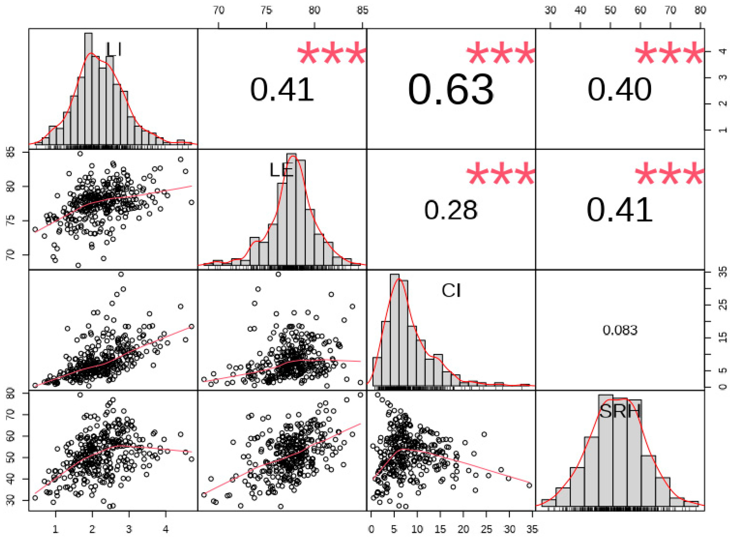
The four human health indicators exhibited significant positive correlations, except for the relationship between Centenarian Index and Self-Rated Health (Figure A1). Life Expectancy was higher in Shanghai, Beijing, and Tianjin, whereas lower in Tibet, Qinghai, and Yunnan (Figure 1a, Table A3). Centenarian Index demonstrated high levels in Heilongjiang, Hainan, and Guangxi, but lower values in Tianjin, Gansu, and Ningxia (Figure 1b, Table A3). Longevity Index exhibited higher values in Hainan, Shanghai, and Guangdong, while lower values were in Gansu, Ningxia, and Shaanxi (Figure 1c, Table A3). Self-Rated Health presented higher values in Guizhou, Zhejiang, and Fujian, whereas lower values in the west of China (Figure 1d, Table A3).

3.2. Model Comparison

We first evaluated the performance of each regression model for the four health indicators (Table 1). The OLS model provided a baseline level of predictive accuracy, whereas the GWR model improved performance by accounting for spatial heterogeneity. The RF model enhanced prediction by capturing nonlinear relationships. Among all models, the GWRF model achieved the highest predictive performance, demonstrating both superior explanatory power and accuracy. Notably, its lower out-of-bag RMSE compared to the RF model underscores the importance of simultaneously considering spatial heterogeneity and nonlinear effects in analyzing human health outcomes.

3.3. The Global and Local Dominant Influencing Factors for Multidimensional Human Health

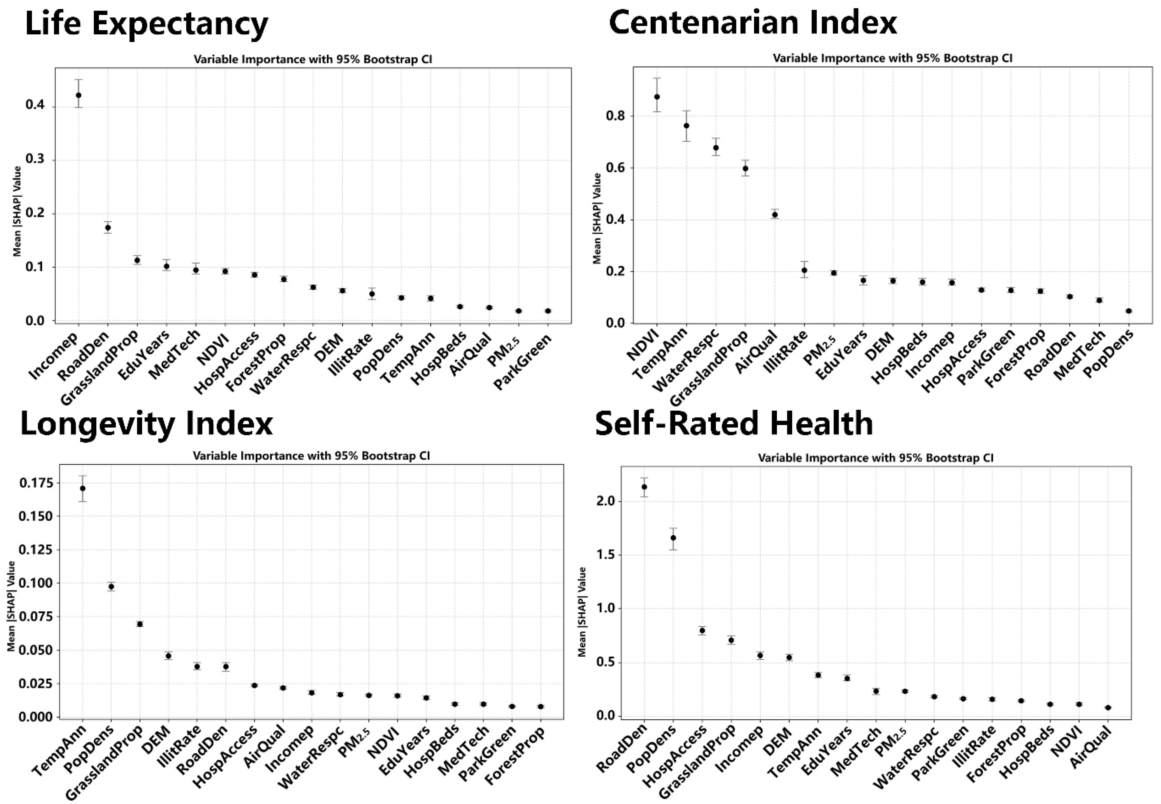
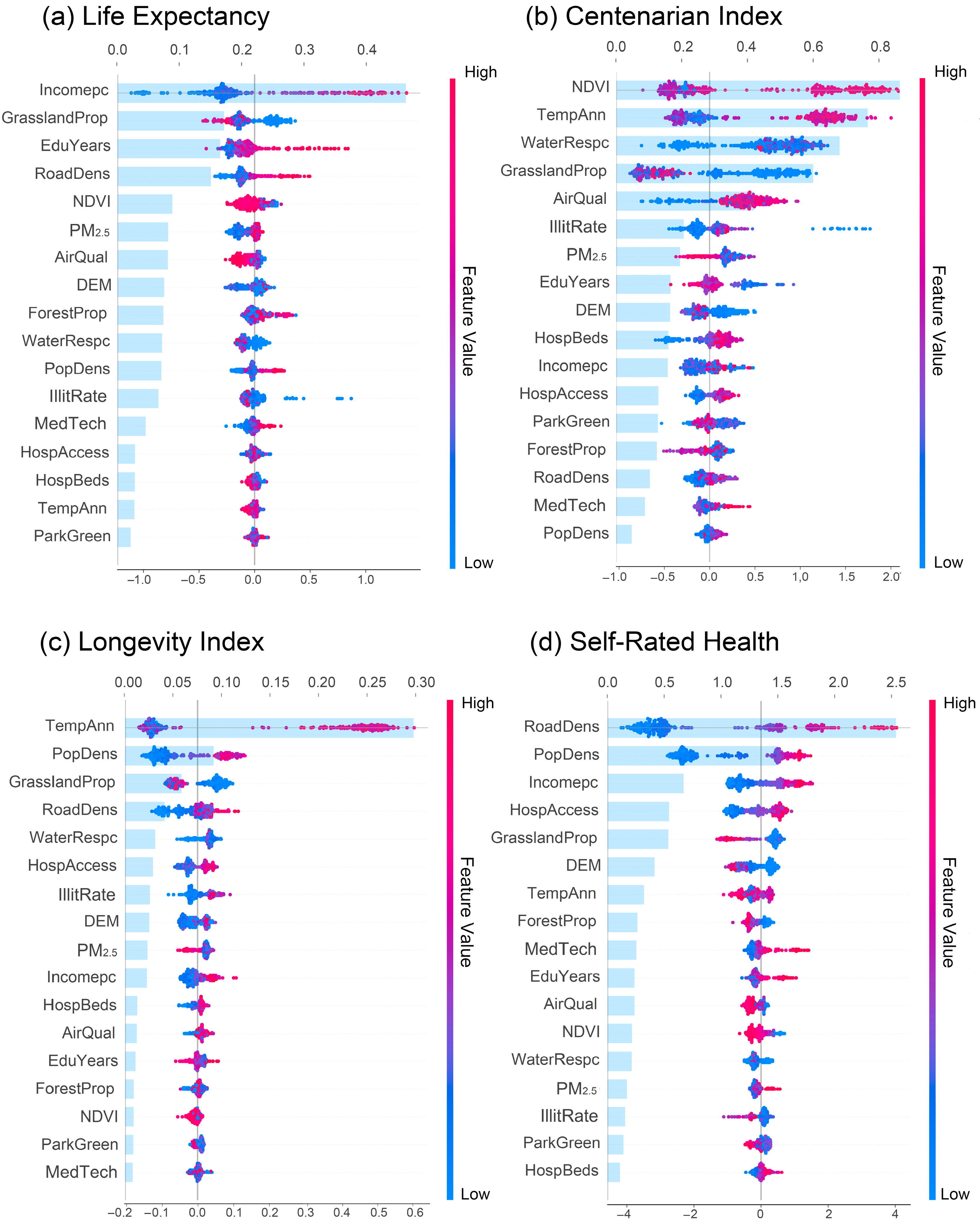
The GWRF model revealed that the dominant influencing factors for the four health indicators differed (Figure 2), and the identified key variables remained consistent in bootstrapped ranking results (Figure A2). We identified the global dominant influencing factors of multidimensional human health by comparing the mean absolute SHAP values derived from the model. Life Expectancy was primarily influenced by Incomepc (|SHAP value| = 0.46), GrasslandProp (|SHAP value| = 0.17), EduYears (|SHAP value| = 0.16), and RoadDens (|SHAP value| = 0.15), with three of the top four factors being socioeconomic factors (Figure 2a). Moreover, most of the socioeconomic factors, such as Incomepc, EduYears, RoadDens, and PopDens, exhibited significant positive impacts on Life Expectancy. Most natural factors, such as GrasslandProp, NDVI, AirQual, and WaterRespc, primarily presented negative impacts.
For extreme health, the Centenarian Index was primarily influenced by NDVI (|SHAP value| = 0.87), TempAnn (|SHAP value| = 0.76), WaterRespc (|SHAP value| = 0.68), GrasslandProp (|SHAP value| = 0.60), and AirQual (|SHAP value| = 0.42), with the top five factors being natural factors (Figure 2b). Improvements in ecological conditions were generally associated with positive impacts. For example, NDVI showed a long red tail on the right, corresponding to higher feature values, and a short cluster of points on the left with lower values. Higher NDVI values corresponding to positive SHAP values indicate that NDVI tends to increase the predicted Centenarian Index relative to the model’s average prediction. Similarly, AirQual also exhibited positive effects. In contrast, PM2.5, as an indicator of environmental pollution, demonstrated a negative impact. TempAnn had the strongest dominant influence on the Longevity Index (|SHAP value| = 0.30), with PopDens (|SHAP value| = 0.09) and GrasslandProp (|SHAP value| = 0.06) also contributing (Figure 2c). Among these, TempAnn and PopDens exhibited significant positive impacts on Longevity Index, while GrasslandProp showed a negative effect.
Self-Rated Health was primarily influenced by RoadDens (|SHAP value| = 2.49), followed by PopDens (|SHAP value| = 1.47), Incomepc (|SHAP value| = 0.66), and HospAccess (|SHAP value| = 0.53) (Figure 2d). The socioeconomic factors demonstrated higher importance and significant positive effects for Self-Rated Health, as reflected by the top four factors. In contrast, natural factors generally showed negative impacts and relatively lower importance, such as GrasslandProp, DEM, and ForestProp.
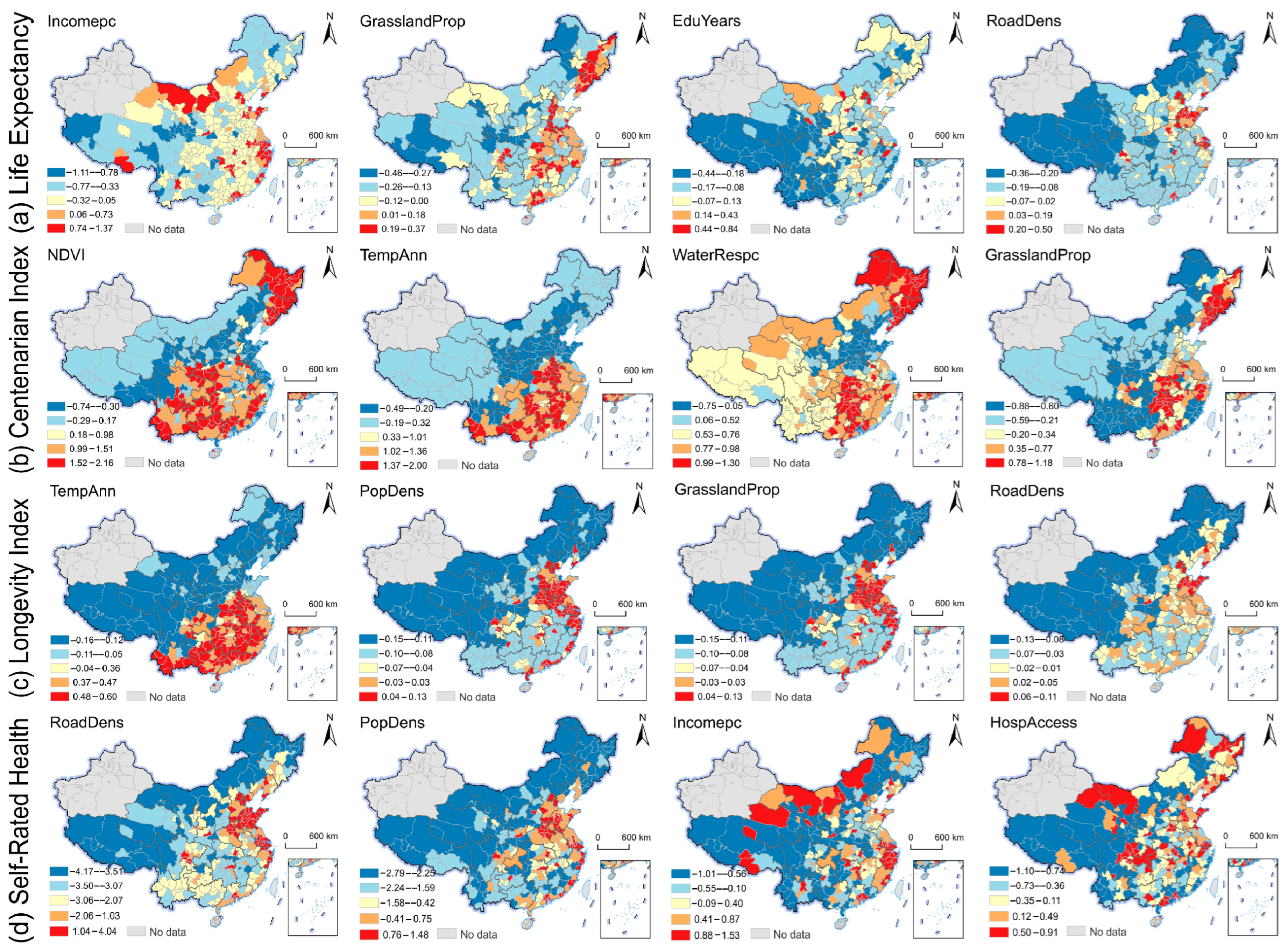
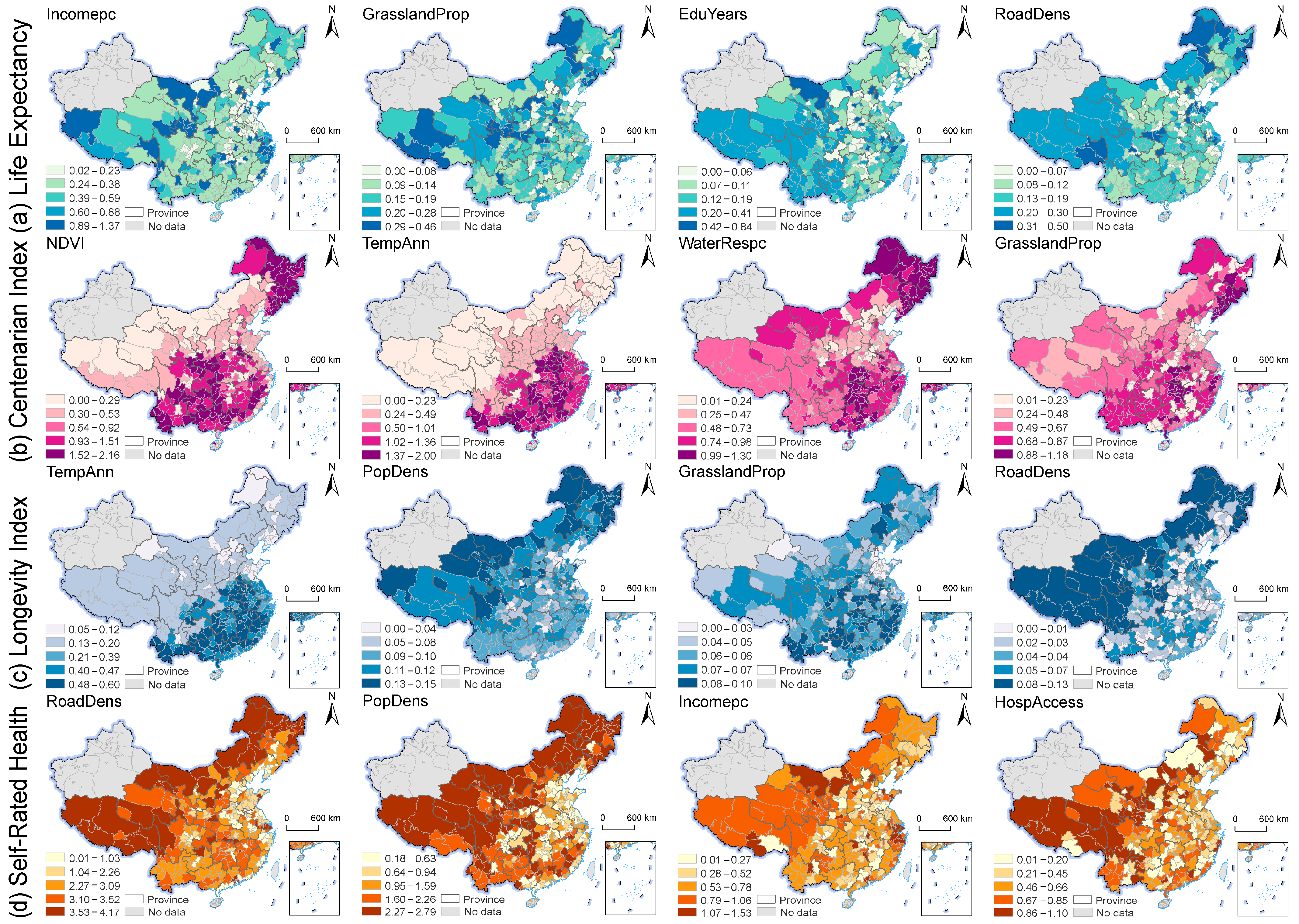
The SHAP values of the identified key variables exhibited varying directions and magnitudes across different regions of China (Figure A3). We mapped the spatial distribution of the absolute SHAP values for selected key variables to identify the local dominant influencing factors (Figure 3). For Life Expectancy (Figure 3a), the impact of Incomepc was spatially dispersed, mainly concentrated in southeastern coastal cities and parts of the northwest. GrasslandProp and RoadDens showed weaker effects in the southeast but stronger impacts in the northwest and northeast. EduYears had a greater influence primarily in the western region. For the Centenarian Index (Figure 3b), NDVI showed stronger effects in southern and northeastern regions. TempAnn exhibited a decreasing influence from the southeast to the northwest. WaterRespc had a greater impact in the northeast and Guangdong, Hubei, and Hunan. The strongest effects of GrasslandProp were concentrated in Jilin, Liaoning, Hubei, and Hunan. For the Longevity Index (Figure 3c), TempAnn and GrasslandProp had greater impacts in the southern region, while PopDens and RoadDens were more important in the north. For Self-Rated Health (Figure 3d), RoadDens and PopDens were also more influential in northern areas, and the spatial pattern of Incomepc was similar to that observed for Life Expectancy. HospAccess showed stronger effects mainly in the western region.

3.4. Nonlinear Effects on Multidimensional Human Health

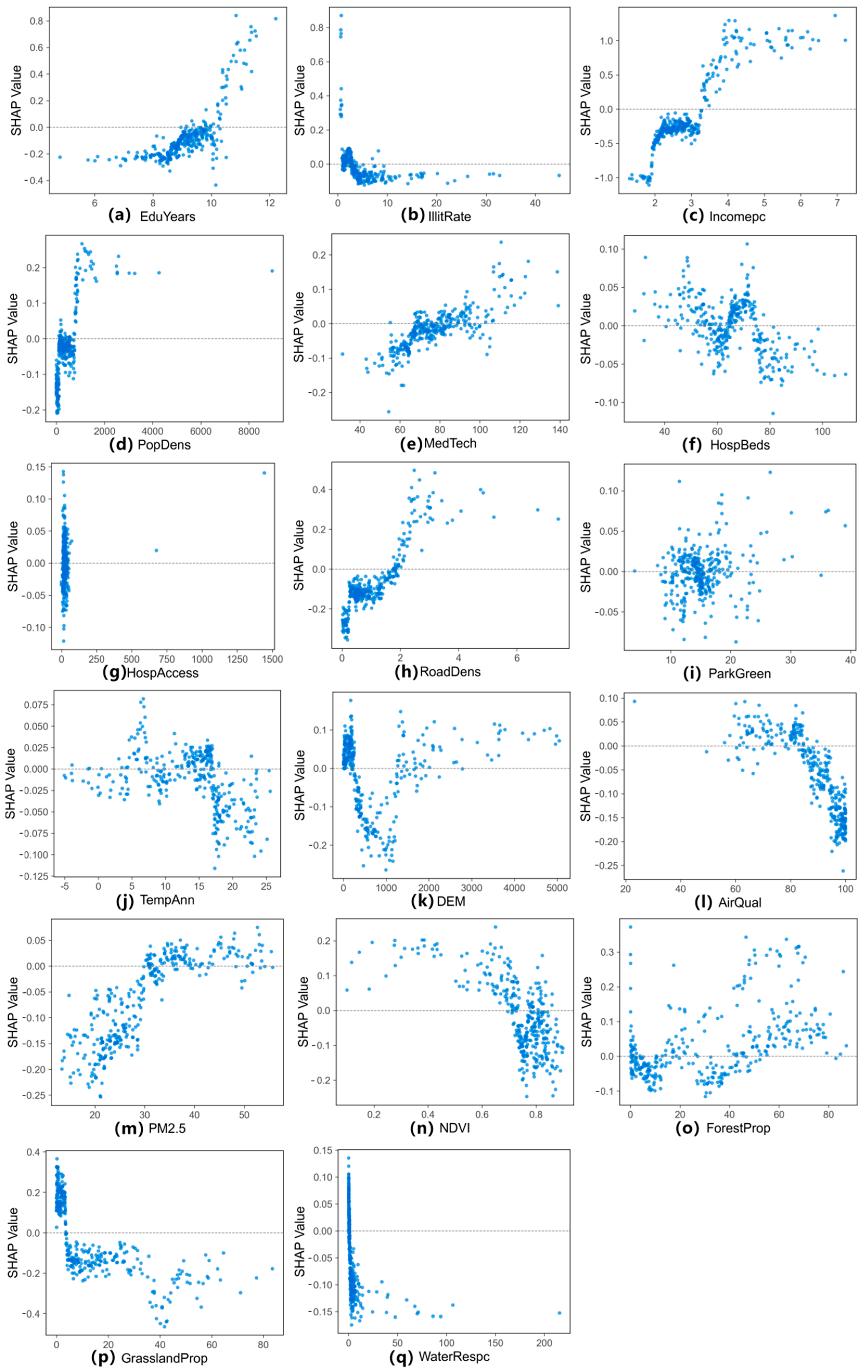
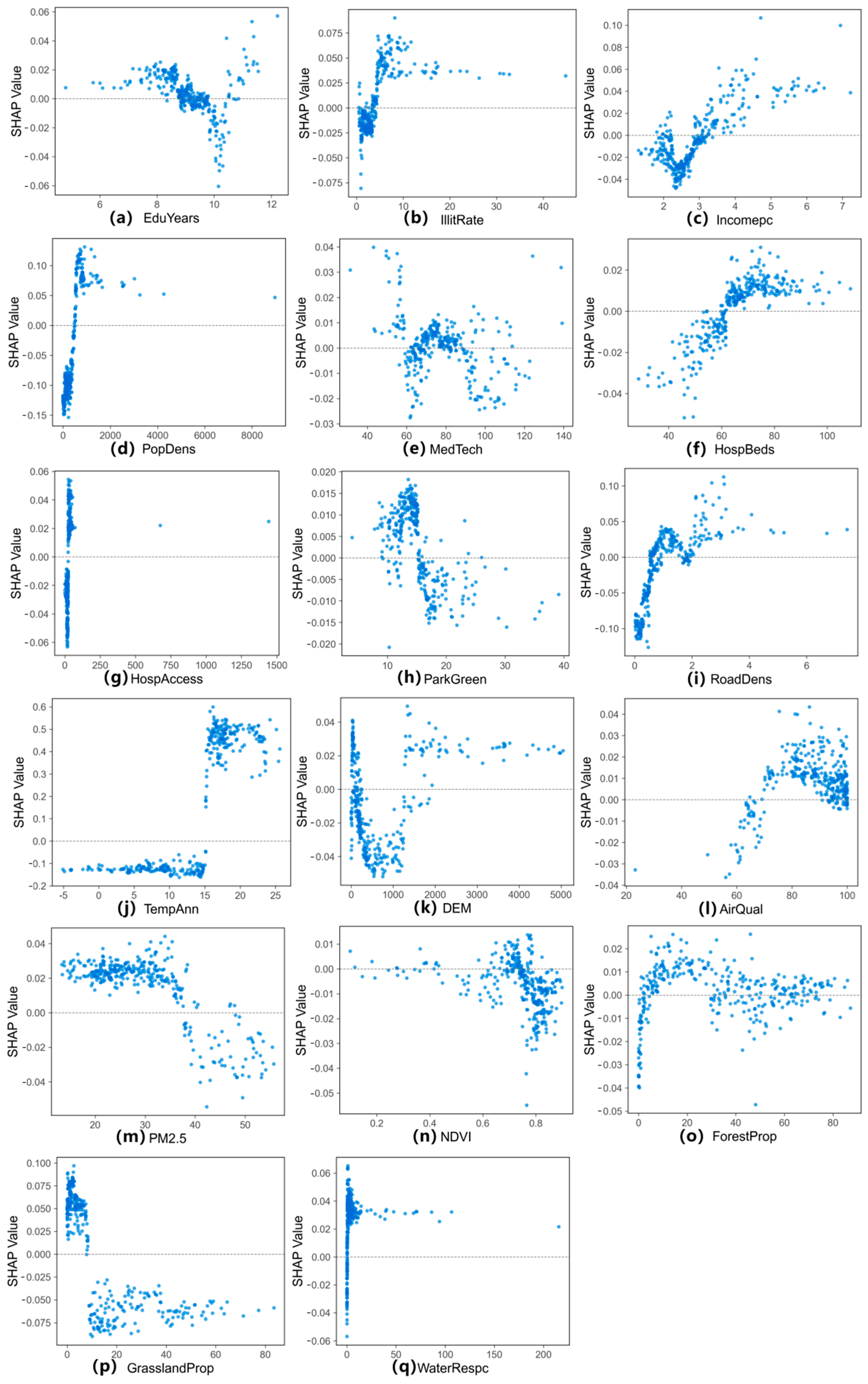
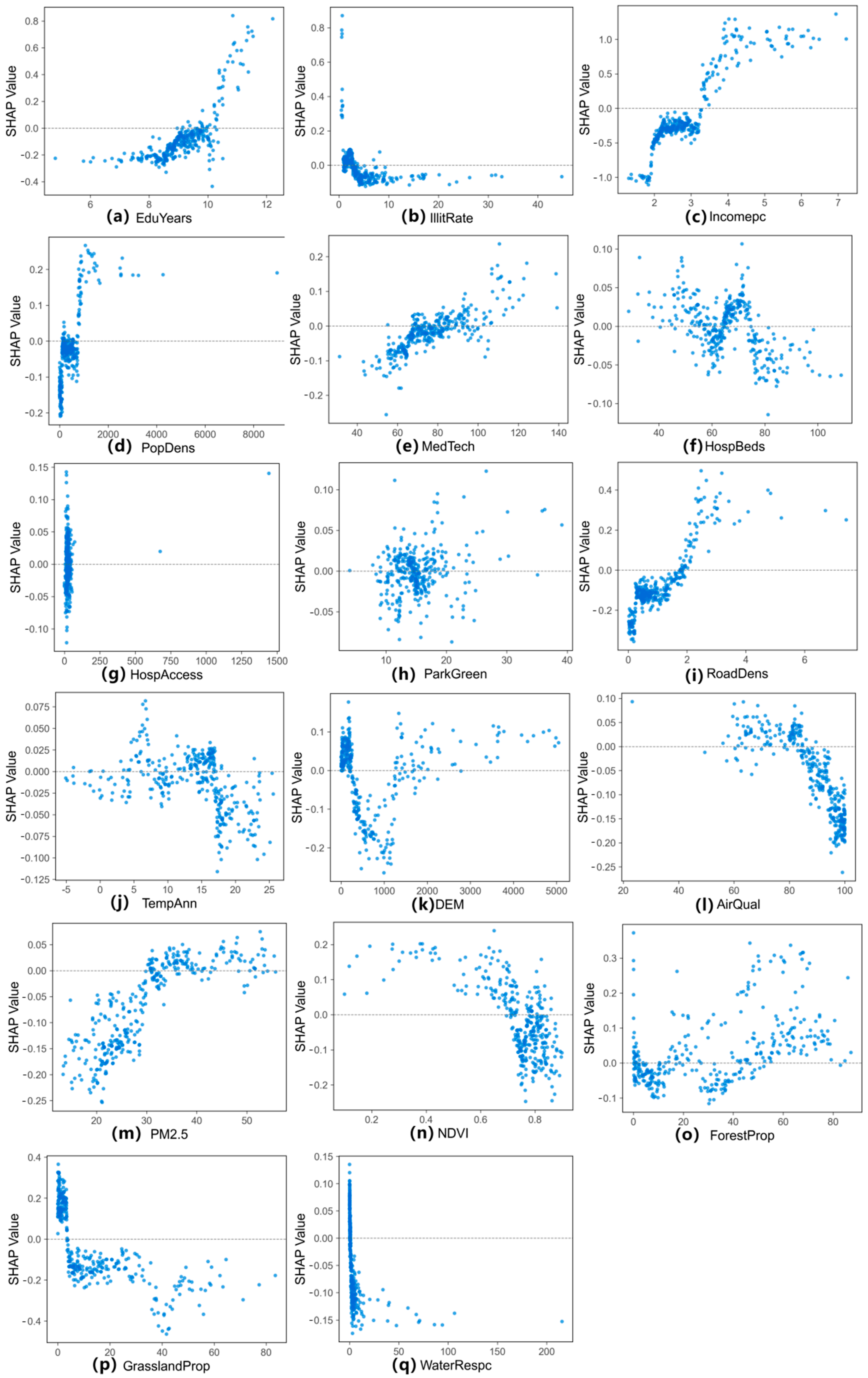
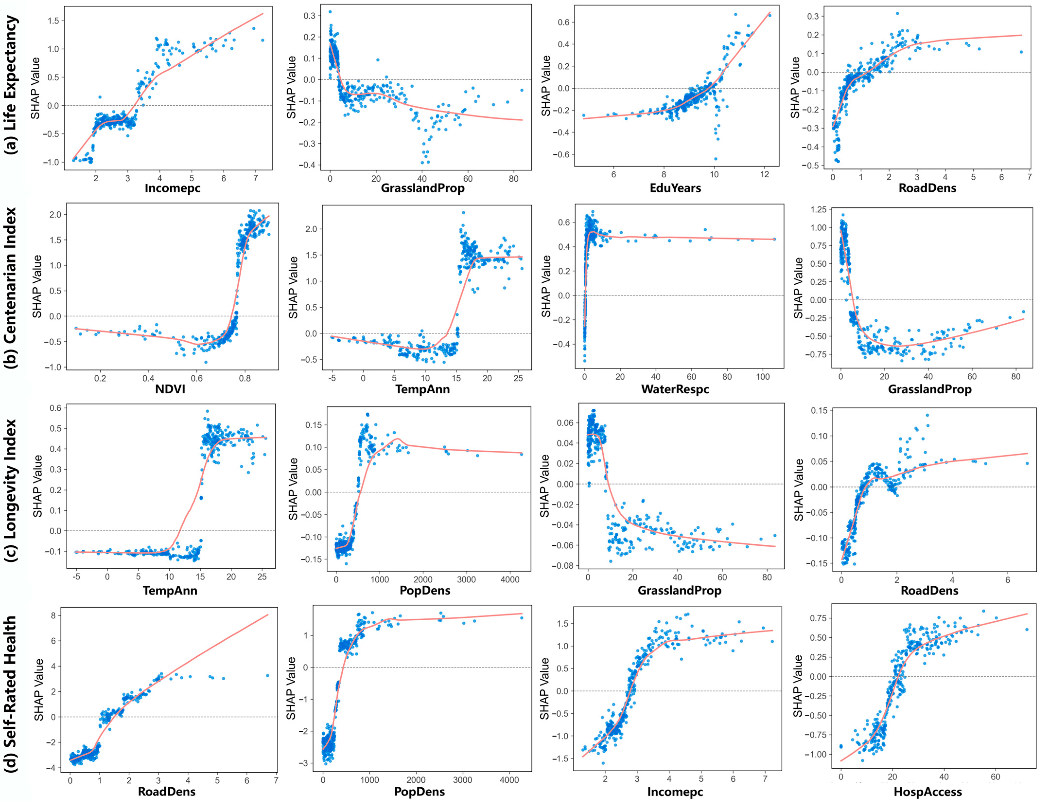
The SHAP-based dependence plots revealed that most variables exhibited nonlinear effects on human health (Figure 4, Figure A4, Figure A5, Figure A6 and Figure A7). For the top four influencing factors, most of them were positively associated with health indicators, except for GrasslandProp (Figure 4).
For Life Expectancy (Figure 4a), the SHAP analysis revealed distinct nonlinear patterns among key predictors. The SHAP value of EduYears increased gradually at first, followed by a sharp rise once EduYears exceeded nearly 9.98 years. Incomepc and RoadDens exhibited similar trajectories: the positive local effects on Life Expectancy tended to plateau when Incomepc reached close to 4.19 × 10⁴ CNY and RoadDens extended to around 3.18 km/km2.
For the Centenarian Index (Figure 4b), the SHAP value of NDVI started from a negative level and increased gradually. A distinct positive effect emerged and rose sharply once NDVI exceeded 0.75. The marginal contribution of WaterRespc to the Centenarian Index followed a “Γ” shape. A rapid increase in SHAP value was observed when WaterRespc was below roughly 2.53 × 10³ m3/person, after which the effect tended to stabilize. For the Longevity Index (Figure 4c), PopDens and RoadDens began to exert positive effects after exceeding thresholds near 473.23 persons/km2 and 0.69 km/km2, respectively. The association of TempAnn with Longevity Index and Centenarian Index followed a similar pattern, with a modest negative effect shifting to a pronounced positive impact at TempAnn approximately 15 °C.
For Self-Rated Health (Figure 4d), the SHAP values of the top four influential variables all exhibited a rapid increase followed by a plateau, indicating a nonlinear but consistently positive relationship. The health benefits associated with increases in RoadDens, PopDens, Incomepc, and HospAccess were most pronounced when these variables were, respectively, below about 3.03 km/km2, 910.47 persons/km2, 3.68 × 10⁴ CNY, and 25.88.

4. Discussion

4.1. What Are the Major Influencing Factors for Multidimensional Human Health?

Human health in China demonstrated great spatial heterogeneity across China (Figure 1). In 2020, Longevity Index and Self-Rated Health were higher in the southeast and lower in the northwest, while the Centenarian Index was elevated in southern and northeastern regions (Figure 1). These patterns remained largely consistent with those observed in 2010 and earlier [15,71], reflecting the persistent nature of spatial health disparities. Socioeconomic inequalities and regional disparities in natural environmental conditions are widely recognized as key drivers of these disparities [4,53,72,73,74]. The structural and long-term features of these inequities, both in the natural environment and in socioeconomic conditions, contribute to the enduring spatial disparities observed in health [27,75,76,77,78]. Correlation analysis further revealed no significant relationship between the Centenarian Index and Self-Rated Health (Figure A1), which may reflect differences in their underlying natural and socioeconomic determinants. Existing studies have shown that the Centenarian Index is only weakly associated with socioeconomic conditions but is more strongly influenced by natural environmental factors [79,80], whereas Self-Rated Health is more closely related to socioeconomic characteristics [81,82,83]. By evaluating multidimensional human health, we found that the spatial distribution of subjective and objective health differed (Figure 1), suggesting different influencing factors for multidimensional human health.
To better capture the nonlinear and spatially heterogeneous nature of health determinants, we combined the GWRF model with the SHAP interpretations. Compared to traditional models (OLS, GWR, RF), GWRF achieved higher R2 values and lower RMSE and MAE values (Table 1), underscoring the necessity of accounting for spatial heterogeneity and nonlinear effects in health-related research. This finding is consistent with previous research [28,32,84]. For example, Grekousis et al. [28] demonstrated that, in the context of COVID-19 mortality across US counties, a Geographically Random Forest model that simultaneously considers spatial heterogeneity and nonlinear relationships outperforms both global models (OLS and RF) and local linear models (GWR). Moreover, the incorporation of SHAP helps overcome the “black-box” limitations commonly associated with machine learning approaches, providing more detailed explanations of the GWRF model [59].
GWRF revealed distinct patterns in the global determinants of multidimensional health (Figure 2). We found that all the top five contributors to the Centenarian Index and two of the top four influencing factors for the Longevity Index fall within the natural domain (Figure 2b,c), suggesting extreme health outcomes were dominated by natural factors, particularly TempAnn. In contrast, three of the top four most important predictors for Life Expectancy and all top four dominant factors for Self-Rated Health fall within the socioeconomic domain (Figure 2a,d), suggesting that average (Life Expectancy) and subjective (Self-Rated Health) health were mainly influenced by socioeconomic changes. This contrast suggests that longevity and exceptional aging are shaped more by long-term environmental exposure, lifestyle, and genetic predispositions than by socioeconomic status [71].

4.2. Do Natural and Socioeconomic Determinants Exert Nonlinear Influences on Multidimensional Human Health?

Prior studies showed that human health was associated with socioeconomic conditions such as quality healthcare availability [85], transportation [3,17], and economic development [14]. By employing the GWRF model, we found that nearly all socioeconomic influencing factors exhibited nonlinear effects (Figure 4). For example, high-income levels (approximately above 3 × 10⁴ CNY) were associated with positive effects across all four health dimensions (Figure A4, Figure A5, Figure A6 and Figure A7), EduYears exhibited a sharply increasing positive effect on Life Expectancy when exceeding approximately 9.98 years (Figure 4a), and HospAccess exhibited a relatively strong positive association with subjective health when surpassing around 25.88 (Figure 4d). These thresholds suggest that targeted interventions in underserved areas may yield significant improvements in human health.
Although natural factors were less influential in explaining life expectancy, they showed greater importance in influencing extreme health outcomes, exhibiting nonlinear relationships (Figure 4b,c). For factors related to climate conditions, prior research found that Chinese “longevity villages” are typically characterized by an annual mean temperature ranging between 8.6 °C and 24.9 °C [86], suggesting that moderate climatic conditions contribute to longevity [52]. Yet, other studies suggest that colder climates might also foster longer life expectancy [87,88]. Our study showed that annual mean temperature (TempAnn) began to exhibit a significant positive effect on extreme health once it exceeded approximately 15 °C (Figure 4b,c), which further supports the hypothesis that warmer climatic conditions may create a more favorable environmental context for healthy aging and longevity. One possible mechanism is that colder temperatures increase the risk of respiratory infections—cold air can irritate the respiratory tract and promote the spread of viruses and bacteria [89]. However, given that many centenarians in this study were born around 1920—a time when heating technologies such as air conditioning were largely unavailable—the protective effect of warmer temperatures may have been more pronounced during their formative years. As living conditions improve, the long-term adverse effects of cold climates may gradually diminish.
In addition, our results showed that lower DEM were generally associated with higher levels of human health, although some high-altitude regions also demonstrated positive effects (Figure A4, Figure A5, Figure A6 and Figure A7). Previous studies have reported mixed findings on the relationship between elevation and human health: some suggest a negative association [23], others highlight potential health benefits or longevity advantages in mountainous areas [86,90], while still others find the effect negligible [71]. These inconsistencies may reflect the complex, nonlinear nature of elevation–health relationships, which vary across regions. Our spatially explicit and nonlinear modeling approach captures these nuanced patterns, thereby reconciling previous contradictory findings and enhancing the robustness and interpretability of our results.
Environmental quality as measured by NDVI demonstrated a weak and negative contribution to the Centenarian Index when below around 0.75, but shifted to a strong positive driver once this threshold is exceeded (Figure 4b). This may be because areas with low greenness often suffer from wind erosion and poor air quality, which negatively impact health. In contrast, highly vegetated environments offer better oxygen levels, stronger air purification capacity, and reduced environmental stress, thereby contributing to increased life spans.
In addition, increases in resource supply do not uniformly enhance health outcomes, for example, a higher proportion of grassland is linked to adverse effects (Figure 4). This counterintuitive result may reflect the dual role of grassland coverage as both a mechanistic and proxy variable. On one hand, grasslands may influence health indirectly by shaping pastoral livelihoods, which are often associated with lower incomes and limited access to healthcare and nutrition. On the other hand, high grassland areas are typically located in China’s northwest, where water scarcity and socioeconomic underdevelopment are prevalent. These co-occurring disadvantages may outweigh any ecological benefits of grassland, resulting in a net negative association with health.

4.3. Implications for Policy Management

Our findings offer several important implications for health-related policy and regional planning. First of all, we found that health management should be tailored to specific health types. While socioeconomic factors (e.g., education and income) are key determinants for average health and subjective health, natural factors play a greater role in extreme health (Figure 2). The varying feature importance can serve as a foundation for determining the priority of intervention measures for different health aspects. Yet, although the effects of socioeconomic factors on longevity are often more observable and well-documented, the influence of natural factors tends to be overlooked. This is partly because tracking longevity requires long-term observation and large, representative samples, which are often lacking. As human health is multidimensional and assessed by over 100 indicators [91], a comprehensive assessment is essential for improving well-being.
Second, effective health policies must be regionally specific. We observed significant spatial heterogeneity in the importance of health determinants. Socioeconomic factors, for example, have a stronger influence in northwestern China (Figure 3), echoing findings from previous studies showing that the health effects of education are particularly pronounced in western regions [14]. This reinforces the value of sustained investment in basic education and regional development policies, such as the Great Western Development Strategy, in improving health and well-being in less-developed areas [92].
Moreover, the identification of nonlinear relationships and threshold effects provides practical guidance for refining policy interventions. For example, the average years of education showed a critical threshold of 9.98 years, beyond which improvements in educational attainment were associated with marked gains in population health (Figure 4a). This highlights the importance of promoting access to higher levels of education as a strategic lever for improving public health. Similarly, the nonlinear effects of HospAccess on subjective health suggest that in regions where HospAccess remains below the threshold of 25.88, efforts should focus on further improving the accessibility and spatial distribution of healthcare resources. While in areas that have already surpassed this threshold, attention should shift toward enhancing the quality, efficiency, and equity of healthcare services to maximize health outcomes. In addition, in economically developed areas, the health benefits of increased RoadDens and PopDens have largely plateaued (Figure 4). These regions may focus more on optimizing the quality and accessibility of existing infrastructure and managing potential negative externalities such as congestion. In contrast, underdeveloped regions may still benefit from improvements in transportation connectivity and population agglomeration to enhance the availability of health services and social resources.

4.4. Limitations and Future Directions

While our study provides a comprehensive and spatially explicit analysis of the determinants of human health—highlighting the relative importance and nonlinear effects of diverse environmental and socioeconomic factors—it is important to acknowledge several limitations. Although high Shapley values indicate that certain features strongly influence the model’s predictions, they do not imply direct causal relationships with the health outcomes [93,94]. These associations may result from unobserved confounders, spatial clustering, or spurious correlations inherent in the data [95]. Therefore, caution is warranted when interpreting SHAP-derived variable importance, especially in complex, observational settings. Furthermore, the underlying mechanisms through which environmental and socioeconomic factors influence health remain insufficiently understood and merit further investigation using causal inference approaches (e.g., structural equation modeling, instrumental variable techniques, or quasi-experimental designs). Future research should also incorporate longitudinal data to better capture temporal dynamics and validate the robustness of these associations over time.

5. Conclusions

This study utilized city-level data from the Seventh National Population Census to provide the most up-to-date assessment of multidimensional human health in China. By integrating GWRF and SHAP models, we uncovered spatial heterogeneity and nonlinear patterns in how socioeconomic and natural factors influence various dimensions of human health. Our results demonstrate substantial differences in determinants of human health: average health (Life Expectancy) and subjective health (Self-Rated Health) were primarily driven by socioeconomic factors, while extreme health indicators (Longevity Index and Centenarian Index) were mainly shaped by natural factors. While the dominant determinants of human health differed across regions, socioeconomic factors tended to play a more significant role in shaping health outcomes in Northwest China. Furthermore, both socioeconomic and natural factors displayed pronounced nonlinear impacts and threshold effects on human health. Our findings advocate for a multidimensional, spatially tailored, and threshold-sensitive approach to health management. Policymakers should prioritize interventions based on the specific health dimension, local context, and critical thresholds of key influencing factors, to more effectively improve population health and reduce regional health disparities.

Author Contributions

Conceptualization, Y.L., L.L. and H.W.; Methodology, Y.L., Z.H. and L.L.; Software, Y.L. and Z.H.; Validation, Z.H.; Formal analysis, Y.L. and Z.H.; Investigation, Y.L. and Z.H.; Data curation, Y.L.; Writing—original draft, Y.L. and Z.H.; Writing—review & editing, Y.L., Z.H., L.L. and H.W.; Supervision, L.L.; Project administration, L.L.; Funding acquisition, L.L. All authors have read and agreed to the published version of the manuscript.

Funding

This research was supported by the National Natural Science Foundation of China (42401370), the Natural Science Foundation of Jiangsu Province (BK20241536), and the MOE (Ministry of Education in China) Liberal arts and Social Sciences Foundation (24YJCZH174).

Data Availability Statement

The original contributions presented in the study are included in the article. Further inquiries can be directed to the corresponding author.

Acknowledgments

We acknowledge the data support from the Land Processes Distributed Active Achieve Center (http://lpdaac.usgs.gov, accessed on 30 August 2024), Resources and Environmental Science Data Platform (http://www.resdc.cn, accessed on 30 August 2024), the National Tibetan Plateau Data Center (http://data.tpdc.ac.cn, accessed on 30 August 2024), National Ecosystem Science Data Center, National Science & Technology Infrastructure of China (http://www.nesdc.org.cn, accessed on 30 August 2024), National Earth System Science Data Center (https://www.geodata.cn, accessed on 30 August 2024).

Conflicts of Interest

The authors declare that they have no known competing financial interests or personal relationships that could have appeared to influence the work reported in this paper.

Appendix A

Table A1. Description of variables.
CategoryCharacteristicsVariablesDefinitionUnitMeanData Source
Human healthObjective healthLife ExpectancyThe average survival time of a specific
population with the same age in the future based on specific mortality level
Year77.53China Population Census Yearbook 2020
Centenarian IndexCentenarians per 100,000 inhabitantsPersons/105 population8.18
Longevity IndexThe ratio between the population above
90 years to those above 65
%2.23
Subjective healthSelf-Rated HealthThe percentage of surveyed elderly individuals who rated their own health status as “healthy”%51.44
Socio-
economic factors
EducationEduYearsAverage years of schoolingYear9.14China Population Census Yearbook 2020
IllitRateIlliteracy rate%4.60
EconomyIncomepcPer capita disposable income of residents 104 CNY2.95Statistical Yearbook and Bulletin
GDPpcPer capita GDP104 CNY6.15
PopulationPopDensPopulation densityPersons/km2451.04China Population Census Yearbook 2020
HealthcareMedTechNumber of medical technical personnel per 10,000 persons/104 population77.19Statistical Yearbook and Bulletin
HospBedsNumber of hospital beds per 10,000 persons/104 population65.68
HospAccessHospital accessibility-29.82[36]
InfrastructureParkGreenPer capita green area of parks m2/person15.28China City Statistical Yearbook
RoadDensDensity of roadskm/km21.10Resource and Environmental Science Data Platform
Natural factorsGeographical conditionTempAnnAnnual average temperature°C14.1[37,38,39,40,41]
HumidAnnAnnual average relative humidity%72.03[42]
PrecAnnAnnual Average Precipitationmm103.16[38,39,43]
SlopeSlope°5.86Resource and Environmental Science Data Platform
DEMDigital Elevation Modelm759.39
Environment qualityAirQualProportion of days with good air quality during a year%87.56Statistical Yearbook and Bulletin
PM2.5Annual PM2.5μg/m330.23[44,45,46]
NPPNet primary productivitygC/m2589.28[47]
NDVIAnnual Maximum NDVI-0.73[48,49]
Resource supplyFarmlandPropFarmland proportion%36.38Resource and Environmental Science Data Platform
ForestPropForest proportion%32.55
GrasslandPropGrassland proportion%13.98
WaterRespcPer capita availability of water resources 103 m3/person5.48China City Statistical Yearbook
Table A2. Optimal parameters of the four GWRF models.
Dependent VariablesBandwidthN_EstimatorsMax_Features
Longevity Index701009
Life Expectancy1201005
Centenarian Index701005
Self-Rated Health801005
Table A3. Provincial average values of health indicators.
ProvinceLife Expectancy (Years)Centenarian Index (Persons/
105 Population)
Longevity Index (%)Self-Rated Health (%)
Beijing82.49 12.76 2.85 62.05
Tianjin81.30 0.39 1.91 55.37
Hebei77.89 5.86 1.86 51.80
Shanxi77.70 4.40 1.84 45.47
Inner Mongolia 77.57 9.07 1.82 44.99
Liaoning78.53 12.78 2.25 52.54
Jilin78.55 10.99 2.14 43.85
Heilongjiang77.43 21.83 2.18 42.72
Shanghai82.55 13.05 3.70 61.80
Jiangsu79.04 9.48 2.68 60.77
Zhejiang 80.06 5.49 2.73 64.16
Anhui77.82 8.05 2.42 50.40
Fujian78.27 7.60 2.84 62.64
Jiangxi77.62 5.33 2.18 60.81
Shandong 79.30 7.93 2.44 58.79
Henan77.70 9.13 2.30 56.11
Hubei77.62 7.30 1.76 48.42
Hunan77.86 5.24 2.24 46.11
Guangdong78.89 8.95 3.20 59.08
Guangxi78.40 14.62 3.17 51.70
Hainan77.91 27.45 4.21 47.34
Chongqing78.56 7.33 2.35 59.76
Sichuan77.46 9.80 2.37 47.16
Guizhou74.99 6.68 1.81 64.45
Yunnan74.42 3.49 2.00 52.63
Tibet71.84 3.92 1.76 34.28
Shaanxi77.04 5.72 1.48 48.45
Gansu75.42 2.62 1.00 40.11
Qinghai73.90 3.54 1.70 36.81
Ningxia76.02 1.97 1.23 41.77
Figure A1. Spearman Correlation coefficients between the four health indicators. LI: longevity index; LE: life expectancy; CI: centenarians per 100,000 inhabitants; SH: percentage of the self-rated health level of the older adults. “***” indicates p < 0.001. The lower triangular panels display pairwise scatterplots, where black circles represent individual observations, and the curves denote fitted nonparametric smoothing lines illustrating the underlying association between each pair of indicators.
Land 14 02324 g0a1
Figure A2. Variable importance from bootstrap analysis.
Land 14 02324 g0a2
Figure A3. Spatial distribution of the SHAP value for the selected key influencing factors.
Land 14 02324 g0a3
Figure A4. SHAP-based dependence plots for Life Expectancy. The collection of points reflects the overall trend of SHAP value variations across the samples.
Land 14 02324 g0a4
Figure A5. SHAP-based dependence plots for Centenarian Index. The collection of points reflects the overall trend of SHAP value variations across the samples.
Land 14 02324 g0a5
Figure A6. SHAP-based dependence plots for Longevity Index. The collection of points reflects the overall trend of SHAP value variations across the samples.
Land 14 02324 g0a6
Figure A7. SHAP-based dependence plots for Self-Rated Health. The collection of points reflects the overall trend of SHAP value variations across the samples.
Land 14 02324 g0a7

References

  1. UN. Transforming Our World: The 2030 Agenda for Sustainable Development. Available online: https://sdgs.un.org/2030agenda (accessed on 30 April 2025).
  2. Modranka, E.; Suchecka, J. The determinants of population health spatial disparities. Comp. Econ. Res. Cent. East. Eur. 2014, 17, 173–185. [Google Scholar] [CrossRef][Green Version]
  3. Khedmati Morasae, E.; Derbyshire, D.W.; Amini, P.; Ebrahimi, T. Social determinants of spatial inequalities in COVID-19 outcomes across England: A multiscale geographically weighted regression analysis. SSM-Popul. Health 2024, 25, 101621. [Google Scholar] [CrossRef] [PubMed]
  4. Tu, Y.; Chen, B.; Liao, C.; Wu, S.; An, J.; Lin, C.; Gong, P.; Chen, B.; Wei, H.; Xu, B. Inequality in infrastructure access and its association with health disparities. Nat. Hum. Behav. 2025, 9, 1669–1682. [Google Scholar] [CrossRef] [PubMed]
  5. Qiu, H.-L.; Chen, H.-Y.; Xie, Y.-T.; Zhou, G.-L.; Yang, K.-Z.; Huang, H.-J.; Jiang, J.-C.; Zhu, X.-Q.; Wang, L.; Yan, K.; et al. Green spaces and preventable disease and economic burdens in China from 2000 to 2020: A health impact assessment study. Landsc. Urban Plan. 2025, 261, 105393. [Google Scholar] [CrossRef]
  6. Cumming, G.S.; Buerkert, A.; Hoffmann, E.M.; Schlecht, E.; von Cramon-Taubadel, S.; Tscharntke, T. Implications of agricultural transitions and urbanization for ecosystem services. Nature 2014, 515, 50–57. [Google Scholar] [CrossRef]
  7. Liu, L.; Fang, X.; Wu, J. How does the local-scale relationship between ecosystem services and human wellbeing vary across broad regions? Sci. Total Environ. 2022, 816, 151493. [Google Scholar] [CrossRef]
  8. Liao, L.; Kong, S.; Du, M. The effect of clean heating policy on individual health: Evidence from China. China Econ. Rev. 2025, 89, 102309. [Google Scholar] [CrossRef]
  9. Xu, L.; Han, H.; Yang, C. Nonlinear relationships and spatial heterogeneity between geographical environment and mental health among middle-aged and older adults in China. Sustain. Cities Soc. 2025, 127, 106459. [Google Scholar] [CrossRef]
  10. Hazucha, M.J.; Lefohn, A.S. Nonlinearity in human health response to ozone: Experimental laboratory considerations. Atmos. Environ. 2007, 41, 4559–4570. [Google Scholar] [CrossRef]
  11. Khojasteh, D.N.; Goudarzi, G.; Taghizadeh-Mehrjardi, R.; Asumadu-Sakyi, A.B.; Fehresti-Sani, M. Long-term effects of outdoor air pollution on mortality and morbidity–prediction using nonlinear autoregressive and artificial neural networks models. Atmos. Pollut. Res. 2021, 12, 46–56. [Google Scholar] [CrossRef]
  12. Martin, M.A.; Green, T.L.; Chapman, A. The Causal Effect of Increasing Area-Level Income on Birth Outcomes and Pregnancy-Related Health: Estimates from the Marcellus Shale Boom Economy. Demography 2024, 61, 2107–2146. [Google Scholar] [CrossRef]
  13. Zhang, L.; Zhou, S.; Kwan, M.-P. A comparative analysis of the impacts of objective versus subjective neighborhood environment on physical, mental, and social health. Health Place 2019, 59, 102170. [Google Scholar] [CrossRef]
  14. Jiang, J.; Luo, L.; Xu, P.; Wang, P. How does social development influence life expectancy? A geographically weighted regression analysis in China. Public Health 2018, 163, 95–104. [Google Scholar] [CrossRef] [PubMed]
  15. Yang, R.F.; Ren, F.; Ma, X.Y.; Zhang, H.W.; Xu, W.X.; Jia, P. Explaining the longevity characteristics in China from a geographical perspective: A multi-scale geographically weighted regression analysis. Geospat. Health 2021, 16, 1024. [Google Scholar] [CrossRef] [PubMed]
  16. Pan, Z.; Wu, L.; Zhuo, C.; Yang, F. Spatial pattern evolution of the health level of China’s older adults and its influencing factors from 2010 to 2020. Acta Geogr. Sin. 2022, 77, 3072–3089. [Google Scholar] [CrossRef]
  17. Song, J.L.; Yu, H.C.; Lu, Y. Spatial-scale dependent risk factors of heat-related mortality: A multiscale geographically weighted regression analysis. Sustain. Cities Soc. 2021, 74, 103159. [Google Scholar] [CrossRef]
  18. Wang, S.B.; Wu, J. Spatial heterogeneity of the associations of economic and health care factors with infant mortality in China using geographically weighted regression and spatial clustering. Soc. Sci. Med. 2020, 263, 113287. [Google Scholar] [CrossRef]
  19. Zhu, H.; Ma, W.; Vatsa, P.; Zheng, H. Clean energy use and subjective and objective health outcomes in rural China. Energy Policy 2023, 183, 113797. [Google Scholar] [CrossRef]
  20. Fall, A.K.D.J.; Migot-Nabias, F.; Zidi, N. Empirical Analysis of Health Assessment Objective and Subjective Methods on the Determinants of Health. Front. Public Health 2022, 10, 796937. [Google Scholar] [CrossRef]
  21. Baji, P.; Bíró, A. Adaptation or recovery after health shocks? Evidence using subjective and objective health measures. Health Econ. 2018, 27, 850–864. [Google Scholar] [CrossRef]
  22. Jung, N.-H.; Lee, C.-Y. Subjective and objective health according to the characteristics of older adults: Using data from a national survey of older Koreans. Medicine 2024, 103, e40633. [Google Scholar] [CrossRef] [PubMed]
  23. Wei, C.; Lei, M.; Wang, S. Spatial heterogeneity of human lifespan in relation to living environment and socio-economic polarization: A case study in the Beijing-Tianjin-Hebei region, China. Environ. Sci. Pollut. Res. 2022, 29, 40567–40584. [Google Scholar] [CrossRef] [PubMed]
  24. Anderson, T.; Herrera, D.; Mireku, F.; Barner, K.; Kokkinakis, A.; Dao, H.; Webber, A.; Merida, A.D.; Gallo, T.; Pierobon, M. Geographical Variation in Social Determinants of Female Breast Cancer Mortality Across US Counties. JAMA 2023, 6, e2333618. [Google Scholar] [CrossRef]
  25. Wang, L.; Wei, B.G.; Li, Y.H.; Li, H.R.; Zhang, F.Y.; Rosenberg, M.; Yang, L.S.; Huang, J.X.; Krafft, T.; Wang, W.Y. A study of air pollutants influencing life expectancy and longevity from spatial perspective in China. Sci. Total Environ. 2014, 487, 57–64. [Google Scholar] [CrossRef] [PubMed]
  26. Liao, L.; Du, M. How digital finance shapes residents’ health: Evidence from China. China Econ. Rev. 2024, 87, 102246. [Google Scholar] [CrossRef]
  27. Yang, T.R.; Liu, W.L. Does air pollution affect public health and health inequality? Empirical evidence from China. J. Clean. Prod. 2018, 203, 43–52. [Google Scholar] [CrossRef]
  28. Grekousis, G.; Feng, Z.; Marakakis, I.; Lu, Y.; Wang, R. Ranking the importance of demographic, socioeconomic, and underlying health factors on US COVID-19 deaths: A geographical random forest approach. Health Place 2022, 74, 102744. [Google Scholar] [CrossRef]
  29. Liu, L.; Wu, J. Space cannot substitute for time in the study of the ecosystem services-human wellbeing relationship. Geogr. Sustain. 2025, 6, 100221. [Google Scholar] [CrossRef]
  30. Gu, T.; Zhao, H.; Yue, L.; Guo, J.; Cui, Q.; Tang, J.; Gong, Z.; Zhao, P. Attribution analysis of urban social resilience differences under rainstorm disaster impact: Insights from interpretable spatial machine learning framework. Sustain. Cities Soc. 2025, 118, 106029. [Google Scholar] [CrossRef]
  31. Georganos, S.; Grippa, T.; Gadiaga, A.N.; Linard, C.; Lennert, M.; Vanhuysse, S.; Mboga, N.; Wolff, E.; Kalogirou, S. Geographical random forests: A spatial extension of the random forest algorithm to address spatial heterogeneity in remote sensing and population modelling. Geocarto Int. 2021, 36, 121–136. [Google Scholar] [CrossRef]
  32. Yi, S.; Li, X.; Wang, R.; Guo, Z.; Dong, X.; Liu, Y.; Xu, Q. Interpretable spatial machine learning insights into urban sanitation challenges: A case study of human feces distribution in San Francisco. Sustain. Cities Soc. 2024, 113, 105695. [Google Scholar] [CrossRef]
  33. Xia, J.; Ye, P. National-scale 1-km maps of hospital travel time and hospital accessibility in China. Sci. Data 2024, 11, 1130. [Google Scholar] [CrossRef] [PubMed]
  34. Peng, S. 1-km Monthly Mean Temperature Dataset for China (1901–2023); National Tibetan Plateau/Third Pole Environment Data Center: Beijing, China, 2019. [Google Scholar] [CrossRef]
  35. Peng, S.; Gang, C.; Cao, Y.; Chen, Y. Assessment of climate change trends over the Loess Plateau in China from 1901 to 2100. Int. J. Climatol. 2018, 38, 2250–2264. [Google Scholar] [CrossRef]
  36. Peng, S.; Ding, Y.; Wen, Z.; Chen, Y.; Cao, Y.; Ren, J. Spatiotemporal change and trend analysis of potential evapotranspiration over the Loess Plateau of China during 2011–2100. Agric. For. Meteorol. 2017, 233, 183–194. [Google Scholar] [CrossRef]
  37. Ding, Y.; Peng, S. Spatiotemporal Trends and Attribution of Drought across China from 1901–2100. Sustainability 2020, 12, 477. [Google Scholar] [CrossRef]
  38. Peng, S.; Ding, Y.; Liu, W.; Li, Z. 1 km monthly temperature and precipitation dataset for China from 1901 to 2017. Earth Syst. Sci. Data 2019, 11, 1931–1946. [Google Scholar] [CrossRef]
  39. Zhang, H.; Luo, M.; Zhan, W.; Zhao, Y. A First 1 km High-Resolution Atmospheric Moisture Index Collection over China; National Tibetan Plateau/Third Pole Environment Data Center: Beijing, China, 2023. [Google Scholar]
  40. Peng, S. 1-km Monthly Precipitation Dataset for China (1901–2024); National Tibetan Plateau/Third Pole Environment Data Center: Beijing, China, 2020. [Google Scholar] [CrossRef]
  41. Wei, J.; Li, Z. ChinaHighPM2.5: High-Resolution and High-Quality Ground-Level PM2.5 Dataset for China (2000–2023); Zenodo: Meyrin, Switzerland, 2023. [Google Scholar] [CrossRef]
  42. Wei, J.; Li, Z.; Lyapustin, A.; Sun, L.; Peng, Y.; Xue, W.; Su, T.; Cribb, M. Reconstructing 1-km-resolution high-quality PM2.5 data records from 2000 to 2018 in China: Spatiotemporal variations and policy implications. Remote Sens. Environ. 2021, 252, 112136. [Google Scholar] [CrossRef]
  43. Wei, J.; Li, Z.; Cribb, M.; Huang, W.; Xue, W.; Sun, L.; Guo, J.; Peng, Y.; Li, J.; Lyapustin, A.; et al. Improved 1 km resolution PM2.5 estimates across China using enhanced space-time extremely randomized trees. Atmos. Chem. Phys. 2020, 20, 3273–3289. [Google Scholar] [CrossRef]
  44. Running, S.; Zhao, M. MOD17A3HGF MODIS/Terra Net Primary Production Gap-Filled Yearly L4 Global 500 m SIN Grid V006. NASA EOSDIS Land Processes DAAC. Available online: https://www.earthdata.nasa.gov/data/catalog/lpcloud-mod17a3hgf-006 (accessed on 30 August 2024).
  45. Dong, J.; Zhou, Y.; You, N. A 30 m Annual Maximum NDVI Dataset in China from 2000 to 2020; National Ecosystem Science Data Center: Beijing, China, 2021. [Google Scholar] [CrossRef]
  46. Yang, J.; Dong, J.; Xiao, X.; Dai, J.; Wu, C.; Xia, J.; Zhao, G.; Zhao, M.; Li, Z.; Zhang, Y. Divergent shifts in peak photosynthesis timing of temperate and alpine grasslands in China. Remote Sens. Environ. 2019, 233, 111395. [Google Scholar] [CrossRef]
  47. Qiu, H.; Li, J.H.; Yu, L.S.; Yu, D.; Hou, Z.L. Analysis of the Life expectancy and the impact of diseases. Popul. J. 2018, 40, 31–39. [Google Scholar] [CrossRef]
  48. MEA. Ecosystems and Human Well-Being: Synthesis; Island Press: Washington, DC, USA, 2005; Volume 5. [Google Scholar]
  49. Chen, X.; de Vries, S.; Assmuth, T.; Dick, J.; Hermans, T.; Hertel, O.; Jensen, A.; Jones, L.; Kabisch, S.; Lanki, T. Research challenges for cultural ecosystem services and public health in (peri-) urban environments. Sci. Total Environ. 2019, 651, 2118–2129. [Google Scholar] [CrossRef]
  50. Liu, L.; Wu, J. Ecosystem services-human wellbeing relationships vary with spatial scales and indicators: The case of China. Resour. Conserv. Recycl. 2021, 172, 105662. [Google Scholar] [CrossRef]
  51. Bayentin, L.; El Adlouni, S.; Ouarda, T.B.; Gosselin, P.; Doyon, B.; Chebana, F. Spatial variability of climate effects on ischemic heart disease hospitalization rates for the period 1989–2006 in Quebec, Canada. Int. J. Health Geogr. 2010, 9, 5. [Google Scholar] [CrossRef] [PubMed]
  52. Robine, J.-M.; Herrmann, F.R.; Arai, Y.; Willcox, D.C.; Gondo, Y.; Hirose, N.; Suzuki, M.; Saito, Y. Exploring the impact of climate on human longevity. Exp. Gerontol. 2012, 47, 660–671. [Google Scholar] [CrossRef] [PubMed]
  53. Liao, L.; Du, M.; Chen, Z. Environmental pollution and socioeconomic health inequality: Evidence from China. Sustain. Cities Soc. 2023, 95, 104579. [Google Scholar] [CrossRef]
  54. Santos-Martin, F.; Martin-Lopez, B.; Garcia-Llorente, M.; Aguado, M.; Benayas, J.; Montes, C. Unraveling the Relationships between Ecosystems and Human Wellbeing in Spain. PLoS ONE 2013, 8, e73249. [Google Scholar] [CrossRef]
  55. Duku, E.; Mattah, P.A.D.; Angnuureng, D.B. Assessment of wetland ecosystem services and human wellbeing nexus in sub-Saharan Africa: Empirical evidence from a socio-ecological landscape of Ghana. Environ. Sustain. Indic. 2022, 15, 100186. [Google Scholar] [CrossRef]
  56. Yee, S.H. Contributions of ecosystem services to human well-being in Puerto Rico. Sustainability 2020, 12, 9625. [Google Scholar] [CrossRef]
  57. Bai, X.M.; Nath, I.; Capon, A.; Hasan, N.; Jaron, D. Health and wellbeing in the changing urban environment: Complex challenges, scientific responses, and the way forward. Curr. Opin. Environ. Sustain. 2012, 4, 465–472. [Google Scholar] [CrossRef]
  58. Wang, W.; Zhang, Y.; Zhao, C.; Liu, X.; Chen, X.; Li, C.; Wang, T.; Wu, J.; Wang, L. Nonlinear Associations of the Built Environment with Cycling Frequency among Older Adults in Zhongshan, China. Int. J. Environ. Res. Public Health 2021, 18, 10723. [Google Scholar] [CrossRef] [PubMed]
  59. Yang, W.; Li, Y.; Liu, Y.; Fan, P.; Yue, W. Environmental factors for outdoor jogging in Beijing: Insights from using explainable spatial machine learning and massive trajectory data. Landsc. Urban Plan. 2024, 243, 104969. [Google Scholar] [CrossRef]
  60. Rodriguez-Galiano, V.; Sanchez-Castillo, M.; Chica-Olmo, M.; Chica-Rivas, M. Machine learning predictive models for mineral prospectivity: An evaluation of neural networks, random forest, regression trees and support vector machines. Ore Geol. Rev. 2015, 71, 804–818. [Google Scholar] [CrossRef]
  61. Liu, K.; Qiao, Y.; Zhou, Q. Analysis of China’s Industrial Green Development Efficiency and Driving Factors: Research Based on MGWR. Int. J. Environ. Res. Public Health 2021, 18, 3960. [Google Scholar] [CrossRef]
  62. Brunsdon, C.; Fotheringham, A.S.; Charlton, M.E. Geographically Weighted Regression: A Method for Exploring Spatial Nonstationarity. Geogr. Anal. 1996, 28, 281–298. [Google Scholar] [CrossRef]
  63. Miao, L.; Liu, C.; Yang, X.; Kwan, M.-P.; Zhang, K. Spatiotemporal heterogeneity analysis of air quality in the Yangtze River Delta, China. Sustain. Cities Soc. 2022, 78, 103603. [Google Scholar] [CrossRef]
  64. Chen, E.; Ye, Z.; Wu, H. Nonlinear effects of built environment on intermodal transit trips considering spatial heterogeneity. Transp. Res. Part D Transp. Environ. 2021, 90, 102677. [Google Scholar] [CrossRef]
  65. Breiman, L. Random Forests. Mach. Learn. 2001, 45, 5–32. [Google Scholar] [CrossRef]
  66. Hamilton, R.I.; Papadopoulos, P.N. Using SHAP Values and Machine Learning to Understand Trends in the Transient Stability Limit. IEEE Trans. Power Syst. 2024, 39, 1384–1397. [Google Scholar] [CrossRef]
  67. Li, Z. Extracting spatial effects from machine learning model using local interpretation method: An example of SHAP and XGBoost. Comput. Environ. Urban Syst. 2022, 96, 101845. [Google Scholar] [CrossRef]
  68. Lundberg, S.M.; Lee, S.-I. A unified approach to interpreting model predictions. Adv. Neural Inf. Process. Syst. 2017, 30, 4765–4774. [Google Scholar] [CrossRef]
  69. Tian, Y.C.; Zhang, Q.; Tao, J.; Zhang, Y.L.; Lin, J.L.; Bai, X.M. Use of interpretable machine learning for understanding ecosystem service trade-offs and their driving mechanisms in karst peak-cluster depression basin, China. Ecol. Indic. 2024, 166, 112474. [Google Scholar] [CrossRef]
  70. Zhang, Y.; Ge, J.; Wang, S.; Dong, C. Optimizing urban green space configurations for enhanced heat island mitigation: A geographically weighted machine learning approach. Sustain. Cities Soc. 2025, 119, 106087. [Google Scholar] [CrossRef]
  71. Wang, S.B.; Luo, K.L.; Liu, Y.L. Spatio-temporal distribution of human lifespan in China. Sci. Rep. 2015, 5, 13844. [Google Scholar] [CrossRef] [PubMed]
  72. Uchiyama, Y.; Kyan, A.; Sato, M.; Ushimaru, A.; Minamoto, T.; Harada, K.; Takakura, M.; Kohsaka, R.; Kiyono, M.; Tsurumi, T.; et al. Association between objective and subjective relatedness to nature and human well-being: Key factors for residents and possible measures for inequality in Japan’s megacities. Landsc. Urban Plan. 2025, 261, 105377. [Google Scholar] [CrossRef]
  73. Marmot, M. Social determinants of health inequalities. Lancet 2005, 365, 1099–1104. [Google Scholar] [CrossRef]
  74. Brulle, R.J.; Pellow, D.N. Environmental Justice: Human Health and Environmental Inequalities. Annu. Rev. Public Health 2006, 27, 103–124. [Google Scholar] [CrossRef]
  75. Flacke, J.; Schüle, S.A.; Köckler, H.; Bolte, G. Mapping Environmental Inequalities Relevant for Health for Informing Urban Planning Interventions—A Case Study in the City of Dortmund, Germany. Int. J. Environ. Res. Public Health 2016, 13, 711. [Google Scholar] [CrossRef]
  76. Dwyer-Lindgren, L.; Kendrick, P.; Kelly, Y.O.; Sylte, D.O.; Schmidt, C.; Blacker, B.F.; Daoud, F.; Abdi, A.A.; Baumann, M.; Mouhanna, F.; et al. Life expectancy by county, race, and ethnicity in the USA, 2000–2019: A systematic analysis of health disparities. Lancet 2022, 400, 25–38. [Google Scholar] [CrossRef]
  77. Sager, L. Global air quality inequality over 2000–2020. J. Environ. Econ. Manag. 2025, 130, 103112. [Google Scholar] [CrossRef]
  78. Eriksson, T.; Pan, J.; Qin, X. The intergenerational inequality of health in China. China Econ. Rev. 2014, 31, 392–409. [Google Scholar] [CrossRef]
  79. Wang, S.; Luo, K.; Liu, Y.; Zhang, S.; Lin, X.; Ni, R.; Tian, X.; Gao, X. Economic level and human longevity: Spatial and temporal variations and correlation analysis of per capita GDP and longevity indicators in China. Arch. Gerontol. Geriatr. 2015, 61, 93–102. [Google Scholar] [CrossRef]
  80. Song, W.; Li, Y.; Hao, Z.; Li, H.; Wang, W. Public health in China: An environmental and socio-economic perspective. Atmos. Environ. 2016, 129, 9–17. [Google Scholar] [CrossRef]
  81. Moon, D.; Pabayo, R.; Hwang, J. An evolution of socioeconomic inequalities in self-rated health in Korea: Evidence from Korea National Health and Nutrition Examination Survey (KNHANES) 1998–2018. SSM-Popul. Health 2024, 26, 101689. [Google Scholar] [CrossRef] [PubMed]
  82. Cullati, S.; Rousseaux, E.; Gabadinho, A.; Courvoisier, D.S.; Burton-Jeangros, C. Factors of change and cumulative factors in self-rated health trajectories: A systematic review. Adv. Life Course Res. 2014, 19, 14–27. [Google Scholar] [CrossRef] [PubMed]
  83. Chen, Y.; Zhang, X.; Grekousis, G.; Huang, Y.; Hua, F.; Pan, Z.; Liu, Y. Examining the importance of built and natural environment factors in predicting self-rated health in older adults: An extreme gradient boosting (XGBoost) approach. J. Clean. Prod. 2023, 413, 137432. [Google Scholar] [CrossRef]
  84. Zhao, H.; Liu, Y.; Yue, L.; Gu, T.; Tang, J.; Wang, Z. Unraveling the factors behind self-reported trapped incidents in the extraordinary urban flood disaster: A case study of Zhengzhou City, China. Cities 2024, 155, 105444. [Google Scholar] [CrossRef]
  85. Qin, J.; Yu, G.; Xia, T.; Li, Y.; Liang, X.; Wei, P.; Long, B.; Lei, M.; Wei, X.; Tang, X.; et al. Spatio-Temporal Variation of Longevity Clusters and the Influence of Social Development Level on Lifespan in a Chinese Longevous Area (1982–2010). Int. J. Environ. Res. Public Health 2017, 14, 812. [Google Scholar] [CrossRef]
  86. Lv, J.; Wang, W.; Li, Y. Effects of environmental factors on the longevous people in China. Arch. Gerontol. Geriatr. 2011, 53, 200–205. [Google Scholar] [CrossRef]
  87. Conti, B. Considerations on temperature, longevity and aging. Cell. Mol. Life Sci. 2008, 65, 1626–1630. [Google Scholar] [CrossRef]
  88. Carrillo, A.E.; Flouris, A.D. Caloric restriction and longevity: Effects of reduced body temperature. Ageing Res. Rev. 2011, 10, 153–162. [Google Scholar] [CrossRef]
  89. Lee, H.J.; Alirzayeva, H.; Koyuncu, S.; Rueber, A.; Noormohammadi, A.; Vilchez, D. Cold temperature extends longevity and prevents disease-related protein aggregation through PA28γ-induced proteasomes. Nat. Aging 2023, 3, 546–566. [Google Scholar] [CrossRef]
  90. Magnolfi, S.U.; Noferi, I.; Petruzzi, E.; Pinzani, P.; Malentacchi, F.; Pazzagli, M.; Antonini, F.M.; Marchionni, N. Centenarians in Tuscany: The role of the environmental factors. Arch. Gerontol. Geriatr. 2009, 48, 263–266. [Google Scholar] [CrossRef]
  91. World Health Organization. WHO Housing and Health Guidelines; World Health Organization: Geneva, Switzerland, 2018. [Google Scholar]
  92. Wu, Y.; Zhang, X. State-led regional development strategy and multidimensional health poverty of the residents: Evidence from the China’s great western development program. Econ. Hum. Biol. 2025, 57, 101494. [Google Scholar] [CrossRef]
  93. Datta, A.; Sen, S.; Zick, Y. Algorithmic Transparency via Quantitative Input Influence: Theory and Experiments with Learning Systems. In Proceedings of the 2016 IEEE Symposium on Security and Privacy (SP), San Jose, CA, USA, 22–26 May 2016; pp. 598–617. [Google Scholar]
  94. Sundararajan, M.; Najmi, A. The many Shapley values for model explanation. In Proceedings of the International Conference on Machine Learning, Virtually, 13–18 July 2020; pp. 9269–9278. [Google Scholar]
  95. Pearl, J. Causality: Models, Reasoning and Inference, 2nd ed.; Cambridge University Press: Cambridge, UK, 2009. [Google Scholar]
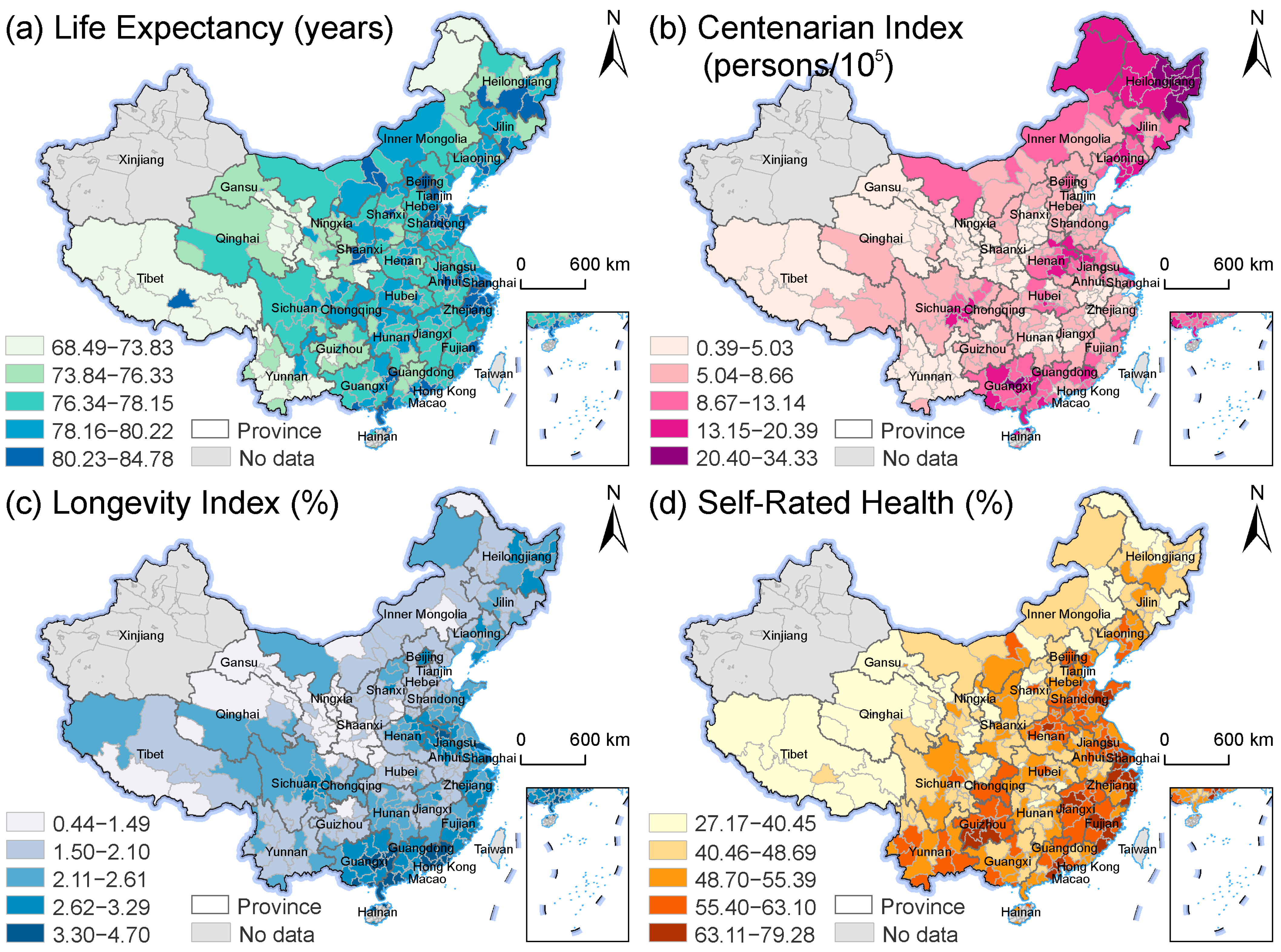
Figure 1. The spatial distribution of Life Expectancy (a), Centenarian Index (b), Longevity Index (c), and Self-Rated Health (d).
Land 14 02324 g001
Figure 2. Beeswarm plots showing the global importance of each determinant on Life Expectancy (a), Centenarian Index (b), Longevity Index (c), and Self-Rated Health (d). The importance of each feature decreases from top to bottom, with each point representing the SHAP value of a sample. The color of the points ranges from blue to red, indicating that the feature values increase from low to high. SHAP values above and below zero indicate positive and negative impacts on human health, respectively.
Land 14 02324 g002
Figure 3. Spatial distribution of the |SHAP value| for selected key influencing factors for Life Expectancy (a), Centenarian Index (b), Longevity Index (c), and Self-Rated Health (d).
Land 14 02324 g003
Figure 4. SHAP-based dependence plots for the selected top four health influencing factors. To better illustrate the main trends in the data, a few outliers were removed from the scatter plots, with the complete version of the plots provided in Figure A4, Figure A5, Figure A6 and Figure A7. The x-axis represents the feature value. Blue dots indicate SHAP values for individual samples, while the curves show the overall dependence trend between feature values and SHAP values.
Land 14 02324 g004
Table 1. The predictive accuracy of the models.
VariablesModelsR2RMSEMAEOOB RMSE
Life ExpectancyOLS0.54 1.68 1.25 /
GWR0.62 1.53 1.16 /
RF0.920.690.511.85
GWRF0.950.570.431.58
Centenarian IndexOLS0.47 3.79 2.94 /
GWR0.76 2.55 1.89 /
RF0.941.230.893.47
GWRF0.970.950.693.04
Longevity IndexOLS0.43 0.52 0.42 /
GWR0.79 0.32 0.25 /
RF0.940.160.130.43
GWRF0.970.120.090.39
Self-Rated HealthOLS0.65 5.55 4.41 /
GWR0.82 4.06 3.25 /
RF0.961.971.545.28
GWRF0.971.581.265.19
Disclaimer/Publisher’s Note: The statements, opinions and data contained in all publications are solely those of the individual author(s) and contributor(s) and not of MDPI and/or the editor(s). MDPI and/or the editor(s) disclaim responsibility for any injury to people or property resulting from any ideas, methods, instructions or products referred to in the content.