Abstract
As a major energy producer and consumer, China has witnessed rapid growth in carbon emissions, which are closely linked to changes in regional climate and the environment. Water, energy, and food (W-E-F) are the three most critical components of human production and daily life, and achieving the coordinated development of these three resources and connecting them with climate change through the carbon emissions generated during their utilization processes has become a key issue for realizing regional ecological sustainable development. This study constructs a dynamic two-stage network slack-based measure-data envelopment analysis (SBM-DEA) model, which integrates the water–energy–food (W-E-F) system with the climate change process to evaluate China’s comprehensive ecological efficiency from 2011 to 2022, and adopts the Dagum Gini coefficient decomposition, kernel density estimation, hierarchical clustering, and geographical detector model to analyze provincial panel data, thereby assessing efficiency patterns, regional differences, and driving mechanisms. The novelty and contributions of this study can be summarized in three aspects. First, it establishes a unified framework that incorporates the W-E-F nexus and climate change into a dynamic network SBM-DEA model, enabling a more systematic assessment of ecological efficiency. Second, it uncovers that interregional overlap effects and policy-driven factors are the dominant sources of spatial and temporal disparities in ecological efficiency. Third, it further quantifies the interactive effects among key driving factors using Geodetector, thus offering practical insights for regional coordination and policy design. The results show that China’s national ecological efficiency is at a medium level. Southern China has consistently maintained a leading position, while provinces in northwest and southwest China have remained relatively backward; the efficiency of the water–energy–food integration stage is relatively high, whereas the efficiency of the climate change stage is medium and exhibits significant temporal fluctuations. Interregional differences are the main source of efficiency gaps; ecological quality, environmental protection efforts, and population size are identified as the primary driving factors, and their interaction effects have intensified spatial heterogeneity. In addition, sub-indicator analysis reveals that the efficiency related to total wastewater, air pollutant emissions, and agricultural pollution shows good synergy, while the efficiency associated with sudden environmental change events is highly volatile and has weak correlations with other undesirable outputs. These findings deepen the understanding of the water–energy–food-climate system and provide policy implications for strengthening ecological governance and regional coordination.
1. Introduction
Since the onset of the Industrial Revolution, the rapid development of the population and economy has led to the consumption of massive amounts of fossil fuels, leading to a sharp surge in global greenhouse gas emissions caused by human activities. The continuous accumulation of these greenhouse gases has created a greenhouse effect, triggering sustained global climate warming. Adverse climate change has heightened risks to human survival and posed potential crises to the socioeconomic development of humanity [1]. People worldwide are confronting the negative impacts of drastic climatic changes, as evidenced by the soaring frequency of extreme weather events—heavy rainfall and floods in Southeast Asia, unprecedented tropical storms in the Gulf region, and unusual snowfall in parts of South Africa and South America—all of which pose significant threats to people’s daily lives and socioeconomic development. How to reduce greenhouse gas emissions and mitigate climate change has become a globally focused topic. In the composition of global carbon emissions, the Asia–Pacific region is currently the dominant area, accounting for over half of the world’s total carbon emissions. Among them, China’s share of carbon emissions is 30.7% of the global total, far exceeding that of other regions [2]. As the world’s largest energy producer and consumer, China’s energy consumption in 2024 reached 5.96 billion tons of standard coal, an increase of 4.3% compared with the previous year. Furthermore, as shown in Figure 1, as one of the world’s major carbon emitters, China’s carbon emissions have exhibited a continuous upward trend [3], and carbon emissions in different provinces are closely associated with their climate and environmental changes.
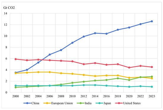
Figure 1.
CO2 total emissions by region, 2000–2023.
Water, energy, and food are fundamental elements in the process of human survival and development. The production and utilization of any one of these three resources closely rely on the supply of the other two, exerting a profound impact on human production, daily life, and the ecological environment. However, ecological pressures brought about by external, uncontrollable factors—such as the steady advancement of urbanization and rapid population growth—constitute key challenges in the development of the contemporary era, and the problems faced by the water–energy–food (W-E-F) system will become increasingly severe. Additionally, the continuous growth of China’s greenhouse gas emissions is closely linked to changes in temperature, precipitation, and the occurrence of sudden environmental events across various provinces in China. Therefore, integrating the W-E-F system with carbon emissions and climate change phenomena to evaluate comprehensive ecological efficiency can effectively reduce environmental pollution and promote the sustainable development of the ecological environment.
Existing studies mainly focus on exploring the interrelationships among the three factors (W-E-F), addressing issues related to the occupation and consumption of water resources in food or energy production processes, and investigating ways to improve resource utilization efficiency. However, they have not yet integrated the W-E-F system with climate change phenomena, leaving room for further expansion in research perspectives. Consequently, this study constructs an evaluation framework for China’s ecological comprehensive efficiency based on the dynamic two-stage network slack-based measure-data envelopment analysis (SBM-DEA) method. This framework separates the W-E-F integration stage from the climate change stage, with carbon dioxide emissions serving as the linking factor between the two. During the research process, methods such as the Dagum Gini coefficient decomposition, kernel density estimation, and Geodetector analysis are comprehensively applied to thoroughly examine the spatiotemporal differentiation characteristics and driving mechanisms of China’s ecological comprehensive efficiency. The three main contributions of this study are as follows: (1) Realizing an integrated analysis of the W-E-F nexus and climate change within a dynamic network SBM-DEA framework; (2) Identifying interregional overlap effects and policy-driven effects as the dominant sources of spatial and temporal disparities; (3) Quantifying the interactive effects among the key driving factors of ecological comprehensive efficiency using Geodetector, thereby providing actionable references for regional coordinated development and policy formulation.
2. Literature Review
2.1. W-E-F System, Carbon Emissions, and Climate Change
The W-E-F system has increasingly been recognized as a critical framework for allocating resources in human economic and social development. Given its interdependent nature, each subsystem within the W-E-F nexus is closely tied to carbon emissions, which in turn are a primary driver of climate change. Therefore, understanding the bidirectional relationship between the W-E-F system and carbon emissions has become a core research focus for promoting global sustainability [4].
First, existing studies reveal that different subsystems of the W-E-F nexus contribute to or mitigate carbon emissions in various ways. Simpson and Jewitt (2019) highlighted that resource allocation and human demand in the water sector directly affect water quality, energy storage, and food security [5]. Mahmood et al. (2022) analyzed land use change in Asia–Pacific countries, arguing that gross domestic product (GDP) growth enhances both energy intensity and economic freedom [6]. From an energy perspective, Mroue et al. (2019) applied an Energy Portfolio Assessment Tool (EPAT) to identify sustainable scenarios that lower carbon emissions within the W-E-F framework [7]. In the agricultural sector, Isaacs et al. (2016) demonstrated that agricultural modernization in Rwanda improved livelihoods but overlooked the multidimensional benefits of diversified planting, calling for more inclusive policies [8]. More integrated approaches, such as those by Yue et al. (2021), employed W-E-F–land–climate optimization models to evaluate the role of food systems in achieving ecological and social co-benefits [9]. Collectively, these findings suggest that the effective utilization of water, energy, and food resources can reduce carbon emissions while improving the resilience and efficiency of the W-E-F system.
Second, carbon emissions also reshape the W-E-F system by driving climate change and altering resource flows. Zhang et al. (2018) argue that shifts in temperature and precipitation influence runoff, crop growth, and energy supply, thereby impacting W-E-F efficiency [10]. Moreover, some scholars have conducted research on a specific climate change event. Kenway et al. (2011) identified urban water as an overlooked factor that significantly affects urban energy use [11]. In addition, Chamas et al. (2021) proposed an extended water–energy–food–carbon (W-E-F-C) optimization model, further integrating carbon footprint management into resource planning [12]. In line with global climate agendas, China has set the dual goals of peaking carbon emissions by 2030 and achieving carbon neutrality by 2060, which require simultaneous transformations in energy use, food production, and water conservation [13].
Third, the climatic impacts of carbon emissions are evident in rising temperatures, altered precipitation patterns, and deteriorating air quality. Horton et al. (2015) and Angélil et al. (2017) emphasized the growing risks of extreme heat waves [14,15], while Chapman et al. (2017) noted intensified warming in urban areas [16]. In terms of precipitation, Sun et al. (2016) and Yu et al. (2018) demonstrated that excessive carbon emissions increase the likelihood of extreme precipitation events [17,18]. The IPCC AR6 assessment suggests that climate change can easily lead to an increase in surface ozone levels in polluted areas. Meanwhile, Fu and Tian (2019) stated that in areas with high anthropogenic emissions, surface ozone concentration increases with temperature [19]. Han et al. (2020) indicated that urbanization coupled with carbon-intensive activities may increase the frequency of pollution episodes [20].
Finally, scholars have also evaluated carbon emission performance and reduction mechanisms to guide governance. Early work by Ramanathan (2002) revealed large cross-country disparities in emission performance [21]. Later, Feng et al. (2015) and Wu et al. (2016) employed DEA-based models to optimize emission reduction allocation, accounting for both collective and individual benefits [22,23]. These methodological innovations provide practical approaches for managing carbon emissions and mitigating climatic impacts.
In summary, the interplay between the W-E-F system and carbon emissions highlights a circular relationship—the W-E-F nexus both influences and is influenced by carbon emissions. Effective governance, therefore, requires integrated approaches that simultaneously optimize resource use, mitigate emissions, and adapt to climate change. However, current research often examines individual subsystems in isolation, overlooking systemic feedback. Future studies should deepen the exploration of integrated W-E-F-C frameworks to enhance resilience and guide sustainable development pathways.
2.2. Influencing Factors on the W-E-F and Climate Change System
The stability and sustainability of the W-E-F system are shaped by a variety of external and internal factors that interact across natural, social, and economic dimensions.
- Natural factors. Climate change [24] and resource endowment [25] significantly affect the spatial and temporal distribution of water, energy, and food resources. Rising CO2 concentrations and precipitation may partly offset the negative effects of temperature increases on crop yields, yet climate variability overall poses substantial challenges to the future stability of the W-E-F nexus [26]. Hydrometeorological gradients, such as elevation and precipitation, also influence system interactions. As these increase, the synergy between water and energy services may weaken, shift into trade-offs, and later strengthen, reflecting the competitive and adaptive dynamics of ecological processes. Photosynthesis, evapotranspiration, and vegetation cover are identified as critical drivers of these interactions [27]. Land-use and land-cover change further exert pressure on the nexus, as shifts in agroforestry, settlements, grasslands, or bare land significantly alter hydrological behavior, energy use patterns, and food production potential [28].
- Socioeconomic factors. Population growth, urbanization, and economic development reshape demand and supply within the W-E-F system. For example, urbanization has been found to negatively correlate with energy consumption in water and food production due to changing resource development decisions [25]. At the same time, GDP is positively associated with water use in both energy and food production, while climate conditions, such as droughts or abundant rainfall, moderate these relationships [29]. Regional economic size [30], population density [31], education level, technology adoption, and effective irrigated area all demonstrate significant spatial heterogeneity in their impacts on W-E-F stress [32]. Furthermore, rapid urban expansion increases the demand for construction land, which intensifies water and energy consumption while reducing arable land, thus threatening food security and ecosystem regulation capacity [33].
- Policy and governance factors. Effective policy frameworks and green development strategies are critical in balancing W-E-F demands. Integrated approaches—such as water–fertilizer irrigation, renewable energy promotion, energy efficiency improvement, crop structure adjustment, and food price stabilization—have been shown to enhance the orderliness and resilience of the W-E-F system [34,35]. In addition, broader economic indicators, including price mechanisms, employment rates, and international trade in resources, also play essential roles in influencing W-E-F security [36]. Renewable energy development (e.g., solar and wind power) can reduce water competition, but large-scale irrigation expansion may exacerbate trade-offs with hydropower demand, underscoring the need for coordinated management strategies [37].
- Systemic interdependencies. Finally, the intrinsic interdependencies among water, energy, and food are defining features of the W-E-F system. Energy production—such as biofuel generation and power plant cooling—requires substantial water resources; water treatment and distribution processes depend on energy inputs; and food production is simultaneously energy-intensive and heavily reliant on irrigation [38]. Understanding these interconnections is vital for developing strategies that mitigate conflicts and promote sustainable, synergistic development.
2.3. Application of the DEA Model and Geodetector in This Field
Recent scholarship has widely employed the DEA framework to examine the W-E-F nexus, especially in China, with notable innovations aligning model designs with policy and governance needs. At the regional scale, DEA has been applied to assess coupling efficiency across provinces from both static and dynamic perspectives [39]. Three-stage DEA frameworks have integrated external drivers such as labor and urbanization, with further extensions embedding ecological sustainability into a “W-E-F-Ecology” nexus [40]. Environmental DEA variants have traced provincial linkages and coupling effects over time [41], highlighting the spatial heterogeneity of subsystem coordination.
Another strand of research links the W-E-F nexus with carbon governance. Here, the zero-sum gains DEA (ZSG-DEA) model plays a central role in emissions-permit allocation, and was originally designed to evaluate efficiency under fixed aggregate outcomes [42]. Methodological refinements have enabled the incorporation of cooperative and competitive interactions between efficient and inefficient units, thereby improving fairness and computational robustness. These advances have informed empirical quota allocations across Chinese provinces [43]. Beyond carbon, DEA has supported broader environmental policy design, such as ZSG-DEA analyses of PM2.5 emissions under capped conditions [44] and comparative efficiency assessments based on production- versus consumption-based accounting of W-E-F resources, providing concrete governance insights [45].
Given escalating climate risks, DEA models that treat CO2 as an undesirable output have become indispensable for evaluating energy and carbon efficiency. Cross-country comparisons in the power sector reveal OECD advantages in carbon performance, though energy efficiency gaps are less significant [46,47]. Plant-level and provincial analyses in China demonstrate dynamic efficiency trajectories, emphasizing the dual goals of carbon mitigation and energy security [48]. Evidence suggests that efficiency gains could reduce provincial energy consumption by approximately 18.4% annually [49]. At the policy scale, DEA results underscore the importance of calibrating carbon metrics to economic development levels to better guide industrial and energy strategies in Asia [50]. Addressing the slack-measurement limitations of traditional DEA, scholars increasingly adopt the slack-based measure (SBM) and its variants, which have revealed that China’s carbon-efficiency improvements lag behind the rationalization of its industrial structure [51].
Complementing DEA, the Geodetector model has gained traction in analyzing spatial heterogeneity and identifying drivers within the W-E-F nexus and related systems. For instance, Tian et al. (2025) constructed a resilience framework for the Yellow River Basin’s W-E-F nexus using grounded theory, the net primary productivity–random forest–particle swarm optimization (NPP-RF-PSO) model, and Geodetector, thereby revealing the processes and mechanisms underlying nexus resilience and spatial differentiation [52]. Similarly, Cao et al. (2025) applied a network SBM model alongside panel quantile regression, the Geodetector, and Mantel tests to evaluate land use efficiency, identifying 11 out of 14 drivers—including carbon neutrality, water consumption, energy use, and food production—as pivotal determinants of efficiency patterns [53].
Beyond the W-E-F nexus, Geodetector has been applied to investigate the heterogeneity of energy transition drivers. Studies integrating Geodetector with geographically weighted regression (GWR) have mapped the spatiotemporal dynamics of China’s energy transition, highlighting regional disparities and the interplay of socioeconomic drivers such as GDP, urbanization, and education level [54]. In urban ecology, Geodetector has been used to evaluate how river proximity and urban morphology shape block-scale thermal environments, with results showing that river distance alone explains 87% of nighttime summer temperature variation, while interactions with urban form increase explanatory power to 96% [55]. Likewise, in remote sensing-based ecological assessments, Geodetector has demonstrated effectiveness in disentangling the explanatory power of land use types and precipitation, while also capturing compounded effects of variable interactions [56].
Overall, DEA and Geodetector complement each other in advancing research on the W-E-F nexus and climate change. DEA provides robust efficiency measurements and policy-oriented insights at multiple scales, while Geodetector offers powerful tools to uncover spatial heterogeneity, interaction effects, and underlying drivers. Together, these methods enrich our understanding of resource-nexus dynamics and inform strategies for sustainable governance and climate adaptation.
3. Data Sources and Research Methods
3.1. Data Source and Indicator System Construction
To provide a clearer overview of the research design, the analytical framework of this study is presented in Figure 2. This framework integrates the efficiency evaluation of both the water–energy–food (W-E-F) integration stage and the climate change stage, as well as the analysis of the driving mechanisms underlying the overall efficiency of these two stages (i.e., ecological comprehensive efficiency).
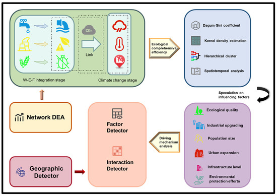
Figure 2.
The research framework of ecological comprehensive efficiency and driving mechanism analysis.
To balance data availability and the research time span, this study uses provincial panel data from China (the study area and its classification are shown in Appendix A) spanning 2011–2022 as the research sample. Figure 3 shows the efficiency research framework and related indicators for the W-E-F integration stage and climate change stage, based on the dynamic two-stage network SBM-DEA model.
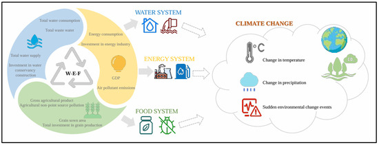
Figure 3.
The research framework of the dynamic two-stage network SBM-DEA model.
The main design idea of the dynamic two-stage network SBM-DEA model proposed in this paper is as follows: The evaluation process of the synergistic effect between the water–energy–food integration system and climate change is divided into two stages, namely, the water–energy–food (W-E-F) integration stage and the climate change stage.
Referring to the approach of Zhang et al. (2024) [57], in the first stage (the water–energy–food integration stage), the inputs include total water supply, water conservancy construction investment, energy consumption, investment in the energy industry, grain-sown area, and total investment in grain production. The outputs are categorized into desirable outputs and undesirable outputs. The undesirable outputs consist of total wastewater, air pollutant emissions, and agricultural non-point source pollution—these are typically associated with negative ecological impacts, as they directly cause the degradation of water, air, and soil (Chen & Liu, 2022 [58]). In contrast, the desirable outputs include gross domestic product (GDP), gross agricultural production, and total water consumption. These reflect positive contributions to ecological efficiency through economic development and improved resource productivity (Sun et al., 2022 [59]; Lee et al., 2024 [60]). Collectively, these indicators fully capture the resource–environment–economy interactions within the water–energy–food system and provide a basis for in-depth research on climate change.
The three basic resource elements—water, energy, and food—affect carbon emissions, which in turn influence climate change. On the one hand, excessive discharge of industrial and chemical wastewater, exploitation and consumption of energy, overuse of pesticides and chemical fertilizers during crop growth, and application of pesticides and chemical fertilizers in grain production all increase carbon emissions. These further trigger the greenhouse effect and pose a threat to regional climate change. On the other hand, the water–energy–food system is of great significance in promoting coordinated development and maximizing resource allocation to mitigate climate change.
Therefore, this paper designates the second stage as the climate change stage. Carbon dioxide emissions generated from the water–energy–food integration system are used as linking indicators, which also serve as input indicators for the climate change stage. Additionally, three climate-related indicators—annual mean temperature change, change in annual precipitation, and sudden environmental change events—are introduced as output indicators for this stage. However, unlike traditional output indicators, annual average temperature change and annual precipitation change function as neutral variables, and their impact on efficiency is non-monotonic—excessive deviations (whether higher or lower) from historical averages may reduce efficiency (Lu et al., 2022 [61]). To capture this characteristic, this study applies the slack-based measure data envelopment analysis (SBM-DEA) model, which is non-radial and non-oriented. The SBM model captures slack variables and penalizes deviations from the ideal state in any direction (Tone, 2001 [62]), thereby enabling both the negative impacts of extreme anomalies in temperature and precipitation and the positive impacts of moderate fluctuations to be reflected in efficiency evaluation. For this reason, following the practice of Lu et al. (2022) [61], this study classifies annual average temperature change and annual precipitation change as desirable outputs. Meanwhile, the inclusion of sudden environmental change events aims to capture negative environmental risks that are often triggered or exacerbated by climate stress. Carbon dioxide emissions from the water, energy, and agricultural sectors, on the other hand, represent the main anthropogenic drivers of climate change. Thus, sudden environmental change events are designated as the only undesirable output in the second stage. The specific descriptions of each indicator are provided in Table 1.

Table 1.
Descriptions of the input and output variables.
3.2. Descriptive Statistics
This study analyzes the trend variations of data for some typical input and output indicators in the first stage (water–energy–food integration stage) and the second stage (climate change stage). For specific details, please refer to Figure 4, Figure 5, Figure 6 and Figure 7.
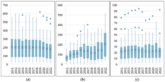
Figure 4.
Statistical analysis of typical variables of the water subsystem of W-E-F integration stage: (a) total water supply, (b) investment in water conservancy construction, and (c) total wastewater.
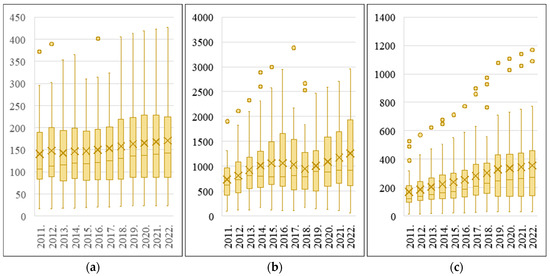
Figure 5.
Statistical analysis of typical variables of the energy subsystem of W-E-F integration stage: (a) energy consumption, (b) investment in the energy industry, (c) GDP.
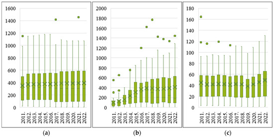
Figure 6.
Statistical analysis of typical variables of the food subsystem of W-E-F integration stage: (a) grain sown area, (b) total investment in grain production, and (c) agricultural non-point source pollution.
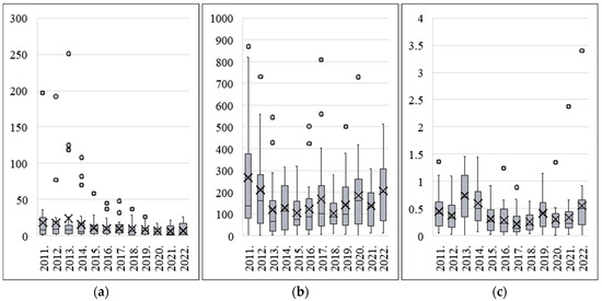
Figure 7.
Statistical analysis of typical variables of climate change stage: (a) sudden environmental change events, (b) change in annual precipitation, and (c) annual mean temperature change.
As shown in Figure 4, in the water subsystem during the W-E-F integration stage, the average total water supply of 30 provinces in China remained generally stable at around 20 billion cubic meters from 2011 to 2017, but showed a gradual decline after 2018, dropping to less than 18 billion cubic meters in 2022. From 2011 to 2015, investment in water conservancy construction increased steadily to about CNY 14 billion, then experienced fluctuations, and finally rose sharply to over CNY 20 billion in 2022, reflecting renewed emphasis on water infrastructure. Wastewater discharge remained around 2.2–2.3 billion tons on average, with peaks in 2015 and 2021, but showed a slight decrease again in 2022.
As shown in Figure 5, in the energy subsystem during the W-E-F integration stage, the average energy consumption of 30 provinces in China remained relatively stable at around 140–150 Mtce from 2011 to 2015, then showed a continuous increase thereafter, reaching over 170 Mtce by 2022. Investment in the energy industry rose steadily before 2015, fluctuated slightly in 2016–2019, and rebounded strongly after 2020, peaking at more than CNY 125 billion in 2022. GDP showed a consistent upward trend throughout the study period, rising from about CNY 17 trillion in 2011 to more than CNY 35 trillion in 2022, with interprovincial gaps gradually widening.
As shown in Figure 6, in the food subsystem during the W-E-F integration stage, the average grain sown area of 30 provinces in China increased steadily from about 3510 thousand hectares in 2011 to over 3930 thousand hectares in 2022, reflecting gradual expansion in agricultural production capacity. Grain production investment rose significantly from around CNY 9.5 billion in 2011 to more than CNY 40 billion in 2022, despite short-term fluctuations between 2018 and 2020. Agricultural non-point source pollution remained relatively stable in the early period, fluctuating around 4.2 billion tons, but increased markedly after 2020, reaching nearly 5 billion tons in 2022, suggesting renewed environmental pressure from intensive farming activities.
As shown in Figure 7, during the climate change stage, the average number of sudden environmental change events across 30 provinces in China decreased significantly, from about 18 cases per year in 2011–2013 to below 7 cases after 2020, reflecting strengthened emergency management and pollution control. Annual precipitation change showed a fluctuating pattern, with relatively high variation in 2011, 2017, and 2020, but smaller deviations in 2015 and 2018; by 2022, the fluctuation level rose again to more than 200 mm. Annual mean temperature change remained relatively moderate overall, with small increases in most years, but recorded a marked rise in 2013 (0.74 °C) and again in 2022 (0.55 °C), suggesting increasing climate volatility in the later period.
3.3. Measure the Level of Ecological Comprehensive Efficiency (Dynamic Two-Stage Network SBM-DEA Model)
This study aims to address the issues arising from static analyses and regional disparities by segmenting the approach into two stages, as follows: the first is the W-E-F integration stage, and the second is the climate change stage. Assuming that there are n DMUs (j = 1, …, n), each with k partitions (k = 1, …, k) and n time periods (T = 1, …, T), each DMU has an input and an output in time period T and a carry-over (link) in the next time period T + 1 to the next time period (j = 1, …, n). The inputs and outputs of each partition K by K (K, h)i denote the divisions from k to h, and n and denote the set of divisions from k and h. We show the inputs and outputs, links, and carry-over definitions as follows:
Inputs and outputs:
: refers to input at time period for division .
: refers to output in time period for division .
Links:
: refers to the period link variable from (b), the process of time during which the scheme is implemented. The following is the conclusion for the period of the scheme of work . Here, represents the number of links from one division to another, while h links refer to the quantity.
Carry-overs:
: refers to the carry-over from time period (t) to period (t+1). This includes the transition from division to division , where represents the number of carry-over items in division .The number of input links for every division is represented by Link . Similarly, Link signifies the number of output links for every division . Each division has a certain number of favorable carry-overs, represented by . Conversely, the number of unfavorable carry-overs for each division is represented by the number of output links for each division, denoted by n .
What follows is the model that is non-oriented.
- Goal function.
Equation (1) defines the overall efficiency of a DMU. It measures how effectively all inputs are converted into desirable outputs while controlling for undesirable outputs. An efficiency value of 1 represents complete efficiency, whereas values less than 1 indicate inefficiency.
Here, and denote the weights assigned to each time period and subsystem , respectively. The numerator captures inefficiencies on the input side, including redundant inputs, linking inefficiencies between subsystems, and inefficiencies in carry-over inputs across periods. Specifically, represents the -th input of subsystem in period , with denoting its input slack. represents the linking variables flowing from subsystem hhh to subsystem , and measures the slack associated with these linkages. is the carry-over input passed from period to period + 1, while indicates its slack.
The denominator reflects inefficiencies on the output side. It incorporates both shortfalls in desirable outputs and excesses in undesirable outputs. In particular, denotes the r-th desirable output of subsystem in period (e.g., GDP, gross agricultural production), with capturing the corresponding output shortfall. Conversely, denotes the undesirable outputs (e.g., wastewater discharge, pollutant emissions), and represents their excesses. The terms and correspond to the number of desirable and undesirable outputs in subsystem .
In this formulation, the efficiency score integrates adjustments from both the input and output dimensions. A value of = 1 indicates that the DMU lies on the production frontier and is fully efficient across all subsystems and time periods. In contrast, values less than 1 imply the presence of input redundancy, linking inefficiency, output shortfalls, or excess undesirable outputs, thus highlighting specific areas of ecological comprehensive inefficiency.
- 2.
- Period and division efficiencies.
The period and division efficiencies are as follows:
i. Period efficiency:
Equation (2) defines the period efficiency, which evaluates the ecological efficiency of all stages within a single time period. This measure highlights temporal variations in performance, showing how efficiency evolves year by year. The notations are consistent with Equation (1), but the focus here is on the efficiency of a given period t, rather than across the entire study horizon.
ii. Division efficiency:
Equation (3) defines the division efficiency, which isolates the performance of each stage (W-E-F integration stage or climate change stage) by aggregating efficiency across all years. This allows the model to identify structural imbalances among subsystems and to reveal which subsystem contributes most to overall efficiency. All variables are defined in Equation (1).
iii. Division–period efficiency:
Equation (4) defines the division–period efficiency, which combines both temporal and subsystem dimensions. It provides the most detailed efficiency measure, pinpointing when (in which year) and where (in which subsystem) inefficiencies occur. This decomposition enables a more precise diagnosis of performance gaps. The notations follow the same definitions as in Equation (1). Table 2 summarizes the key variables used in Equations (1)–(4).

Table 2.
Key variables used in the equations.
To address any potential biases in traditional efficiency indicators, we use the total-factor efficiency index. This index includes eight crucial efficiency models, as follows: total water supply, investment in water conservancy construction, energy consumption, investment in energy industry, grain sown area, total investment in grain production, total water consumption, total wastewater, GDP, air pollution emissions, gross agricultural product, and agricultural non-point source pollution. built-up area, total energy consumption, industrial land area, residential land area, annual mean temperature change, change in annual precipitation, and sudden environmental change events. Efficiencies are equal to 1 when the planned inputs align with the actual inputs, indicating complete efficiency. However, when the planned inputs are less than the actual inputs, efficiencies fall below 1, denoting overall inefficiency.
When the target desirable outputs match the actual desirable outputs, efficiency equals 1, signifying complete efficiency. Conversely, when the target desirable output exceeds the actual desirable outputs, efficiencies fall below 1, indicating overall inefficiency.
3.4. Dagum Gini Coefficient
As a more adaptive inequality measurement tool, the Dagum Gini coefficient demonstrates significant advantages through its three-layer decomposition framework. It can not only systematically deconstruct the overall regional gap into three dimensions, namely, the intraregional gap (), interregional gap (), and super-variable density (), to accurately identify the core sources of the gap, but also effectively avoid measurement distortion caused by sample overlap by deeply capturing the distribution characteristics of each sub-sample. This study also utilizes this method to analyze the composition of regional differences in China’s ecological comprehensive efficiency, and Formula (5) is as follows:
The intragroup gap reflects the disparity in the internal level among different regions within a group; the intergroup gap reflects the disparity in levels between different groups of regions; and the super-variable density reflects the degree of overlap and intersection across different regions, representing the situation of relative disparity.
The calculation formula for the overall Gini coefficient is given by Formula (6), as follows:
among them, n is the number of DMUs; is the average value of China’s ecological comprehensive efficiency; k is the number of regional divisions; represents the ecological comprehensive efficiency of the i-th DMU in the j-th region; denotes the ecological comprehensive efficiency of the r-th DMU in the h-th region; is the number of DMUs in the j-th region; and is the number of DMUs in the h-th region. The calculation formula for (the contribution of intraregional disparity) is given by Formula (7), as follows:
among them, , , and . is the intraregional Gini coefficient of the j-th region. The calculation formula for is given by Formula (8), as follows:
among them, ; further, the contribution rate of super-variable density can be obtained, as shown in Formula (9):
among them, represents the relative impact between the j-th DMU and the h-th DMU; is the difference in the ecological comprehensive efficiency of DMU regions, which can be understood as the mathematical expectation of the total of all sample values, where between the j-th region and the h-th region; is the first-order moment of super-variation, representing the mathematical expectation of the total of all sample values, where between the j-th region and the h-th region; and is the cumulative density distribution function of the h-th (j-th) region. The corresponding calculation formulas for , , and are given by Formula (10), as follows:
among them, , .
3.5. Kernel Density Estimation
In this paper, the Gaussian kernel density function is used to analyze the dynamic distribution and evolution trend of ecological comprehensive efficiency, and the expression of the function is as follows:
where denotes the kernel density estimator, denotes the kernel function, is the sample observation, represents the mean of observations, refers to the sample size, and is the optimal bandwidth.
3.6. Hierarchical Clustering Analysis Based on Euclidean Distance Using the Complete Linkage Algorithm
In this paper, the Euclidean distance metric is first adopted to measure the similarity between samples. The formula is expressed as follows:
among them, n represents the dimension, and , denote the coordinates of the two points in the i-th dimension.
On this basis, the complete linkage algorithm is introduced as the clustering criterion in hierarchical clustering analysis. The distance between two clusters A and B is defined as the maximum distance between all pairwise points belonging to the two clusters, which can be expressed as follows:
where and are two clusters, and represents the Euclidean distance between sample in cluster and sample in cluster .
In the hierarchical clustering procedure, each sample is initially regarded as an independent cluster. Then, according to the complete linkage criterion, the two clusters with the smallest intercluster distance are successively merged until all samples are aggregated into one cluster, thereby forming a hierarchical clustering tree (dendrogram). The complete linkage method tends to maximize inter-cluster heterogeneity while ensuring higher homogeneity within clusters. It must be noted that experimental data usually need to be standardized before clustering. However, all types of efficiency values studied in this paper are inherently in the range of 0 to 1, so no additional standardization is required.
3.7. Geographical Detector Model
To analyze the driving factors of China’s ecological comprehensive efficiency, the Geodetector model is employed for the analysis, and the formula is as follows:
where represents the proportion of variance explained by the factor, represents the types of factors, and , respectively, denote the total sample size and the sample size of stratum , refers to the class interval of the dependent variable or influencing factors , and , respectively, refer to the variance of in the entire study area and within stratum .
In line with the model’s requirements, this study discretizes six driving factors—ecological quality, industrial upgrading, population size, urban expansion, infrastructure level, and environmental protection efforts—using the K-means clustering method. This ensures that intraclass variance is minimized and interclass variance maximized, thereby achieving effective stratification. The clustering results clearly demonstrate spatial heterogeneity; for example, ecological quality is consistently higher in southern provinces but weaker in northern and northwestern regions; industrial upgrading shows coastal provinces in higher strata and inland provinces in lower ones; population size separates highly populated provinces such as Henan, Shandong, and Guangdong into distinct classes, while western provinces remain sparsely populated; urban expansion is concentrated in megacities and coastal areas, with inland regions showing slower growth; infrastructure level is markedly higher in the east and central provinces than in the west; and environmental protection efforts are uneven, with higher categories appearing in provinces along major river basins while others remain at lower levels.
Table 3 confirms the existence of spatial heterogeneity in the research objects of this study and the feasibility of discretization. This is consistent with the methodological assumptions of the geographical detector and provides a solid foundation for subsequent factor detection.

Table 3.
Field difference analysis of the clustering results of six driving factors.
4. Empirical Analyses
4.1. Assessment of Ecological Comprehensive Efficiency Results in China
As shown in Figure 8a, from 2011 to 2022, the total efficiency values of 30 provinces in China exhibited the characteristic of significant regional differentiation. The national average total efficiency value was approximately 0.8179, indicating an overall good performance. Among these provinces, 18 had a total efficiency value exceeding 0.8, accounting for 60% of the total, while one province (Shanghai) achieved a state of full efficiency with a total efficiency value of 1. From the perspective of China’s seven major geographical divisions, there were notable differences in efficiency across regions. South China performed the best, with an average total efficiency value as high as 0.85; in contrast, Southwest China ranked the lowest in the country in terms of total efficiency value, with an average total efficiency value of only 0.68.
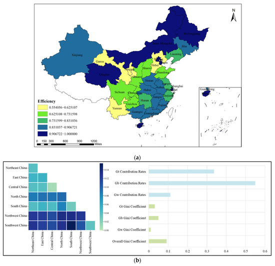
Figure 8.
Spatial distribution and differences of China’s ecological comprehensive efficiency: (a) spatial distribution; (b) decomposition of the Dagum Gini coefficient.
To further explore the regional difference pattern of China’s ecological comprehensive efficiency, this study introduces the Dagum Gini coefficient for analysis. As shown in Figure 8b, the decomposition results of the Dagum Gini coefficient for ecological comprehensive efficiency present the characteristic relationship “contribution rate of hyper-variable density > contribution rate between groups > contribution rate within groups”. This indicates that the dominant source of the overall difference in ecological comprehensive efficiency is the overlapping factors between regions; the impact of the development gap between regions takes second place, and the internal difference within regions has the weakest explanatory power for the overall difference. From the difference decomposition of the Gini coefficient, in terms of the intragroup difference dimension, the intragroup Gini coefficient of the Northwest region has continuously remained at the highest level, which may be due to the existence of negative factors such as ecological fragility in some provinces of the Northwest region. The North China and East China regions follow closely; the intragroup Gini coefficient of the Central China region is the smallest, which may be because the industrial upgrading in the Central China region has strong synergy, and the gap between urban and rural infrastructure is small. In the intergroup difference dimension, the Gini coefficient between the Southwest and South China regions is significantly higher than that of other intergroup combinations, corresponding to the largest gap in ecological comprehensive efficiency, which may be affected by factors such as their ecological conditions and industrial structures. The Gini coefficient between the Central China and Northeast China regions is the smallest, indicating that the difference in their ecological comprehensive efficiency is relatively small.
4.2. Stage Efficiency Analysis
4.2.1. Efficiency Analysis of Water–Energy–Food Integration Stage (S1)
In the W-E-F integration stage, as shown in Figure 9a, China performed well in terms of efficiency values from 2011 to 2022, with an average total efficiency value of approximately 0.8712. The average overall efficiency value of all provinces exceeded 0.5, and more than half of the provinces had an efficiency value of 0.8 or above, while 50% of the provinces achieved an average efficiency value of 1. The average efficiency value in the South China region was 1, showing the best performance, whereas the average efficiency values in the northwest and southwest regions were 0.7589 and 0.6562, respectively, indicating relatively poor performance.
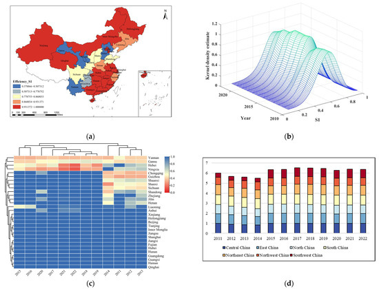
Figure 9.
Spatiotemporal differentiation characteristics and clustering of efficiency in the water–energy–food integration stage: (a) spatial distribution of provincial efficiency; (b) kernel density estimation of efficiency evolution; (c) hierarchical clustering heatmap of provincial efficiencies; (d) regional efficiency comparison over time.
Figure 9b illustrates the kernel density estimation of provincial efficiency during the W-E-F integration stage from 2011 to 2022. In the early years (2011–2015), the distribution was concentrated in the 0.3–0.5 range, reflecting the prevalence of medium-to-low efficiency across provinces. Between 2016 and 2020, the peak gradually shifted toward higher efficiency values (0.5–0.7), and a clear “double-peak” structure emerged, suggesting that while some provinces achieved efficiency breakthroughs, others lagged due to ecological constraints and industrial path dependence. After 2020, the distribution trend became more dispersed, with the higher peak becoming more prominent by 2022, indicating the gradual formation of a stable high-efficiency group alongside a shrinking cluster of low-efficiency provinces.
Figure 9c shows the hierarchical clustering heatmap of provincial efficiencies. High-efficiency provinces in the east remained clustered together, while central and western provinces such as Sichuan, Shaanxi, and Hubei displayed steady improvements but remained independent in the clustering pattern. Southwest provinces, including Yunnan and Guizhou, were far from the high-efficiency group, highlighting persistent regional disparities.
Figure 9d presents a comparison of efficiency performance across China’s seven geographic regions. South China consistently outperformed other regions, while Southwest and Northwest China lagged throughout the study period. These trends also reflect the positive influence of national ecological civilization policies introduced in 2015, which significantly improved integration efficiency at the national level.
4.2.2. Efficiency Analysis of Climate Change Stage (S2)
In the climate change stage, as shown in Figure 10a, China’s average efficiency value from 2011 to 2022 was 0.4360, which was average. The efficiency value in the South China region was the best, with an average efficiency value of 0.8 or above. The efficiency value in the southwest region was the worst, with an average efficiency value of less than 0.35. Moreover, 40% of provinces had an average efficiency value of 0.5 or above; only 4 provinces had a stable average efficiency value of 1, while the efficiency values in most other regions fluctuated greatly.
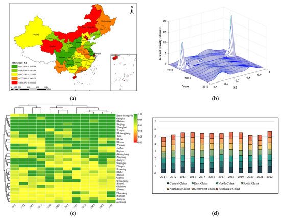
Figure 10.
Spatiotemporal differentiation characteristics and clustering of efficiency in the climate change stage: (a) spatial distribution; (b) kernel density estimation; (c) hierarchical clustering heatmap of provincial efficiencies; and (d) regional efficiency comparison over time.
Figure 10b illustrates the kernel density estimation of provincial efficiency during the climate change stage from 2011 to 2022. In the early period (2011–2013), efficiency values were concentrated at the lower end of the distribution, indicating that most provinces were at a low efficiency level. Between 2014 and 2016, a distinct peak emerged in the medium efficiency range, showing that some provinces improved their performance. After 2017, a second peak appeared in the higher efficiency range (around 0.7–0.9), reflecting the gradual emergence of a high-efficiency cluster, while many other provinces remained at lower efficiency levels. During 2021–2022, the higher peak became more stable and pronounced, suggesting that a group of provinces consolidated their efficiency gains, though the persistence of a low-efficiency cluster indicates continued regional divergence.
Figure 10c shows the hierarchical clustering heatmap of provincial efficiencies. Provinces such as Guangdong, Beijing, and Hainan maintained long-term high efficiency and clustered together, while central and western provinces, such as Sichuan and Shaanxi, displayed moderate improvements. Provinces in the Northwest and Southwest, including Gansu and Yunnan, are located far from the high-efficiency cluster, highlighting persistent spatial disparities in climate change efficiency.
Figure 10d presents a regional comparison of efficiency levels over time. South China consistently maintained the highest efficiency, followed by East and North China, while Southwest and Northwest China remained at the lowest levels throughout the study period. The overall improvement after 2015 reflects the positive influence of ecological civilization policies, which helped accelerate efficiency gains across several regions, despite persistent regional heterogeneity.
4.3. Sub-Variable Efficiency Analysis
Overall, the efficiency performance of the first-stage indicators remained relatively stable, with most provinces achieving high efficiency in multiple years. In contrast, the second-stage indicators displayed larger fluctuations due to the impact of climate variability and policy adjustments. This stage-specific distinction suggests that resource utilization and pollution control in the first stage are more structurally constrained, whereas environmental and climate-related indicators in the second stage are more sensitive to external shocks.
Figure 11 presents a clustered heatmap of sub-indicator efficiencies of undesirable outputs across the two stages in 30 provinces in China from 2011 to 2022. This heatmap was constructed based on the complete linkage algorithm and the Euclidean distance method. Regarding individual indicators, the efficiency of energy consumption in the first stage was generally high, with a majority of provinces reaching an efficiency value of 1 in the mid-to-late study period. Similarly, both total wastewater (TWW) and agricultural non-point source pollution (ANP) maintained relatively high efficiency, though with certain interprovincial differences. Air pollutant emissions (APEs) also showed improving performance over time, and by 2020–2022, more than half of the provinces had achieved efficiency values close to 1. In contrast, temperature change efficiency values fluctuated considerably, with fewer than two-thirds of provinces maintaining efficiency above 0.5. Sudden environmental change events demonstrated greater uncertainty—although some provinces showed low efficiency in the early years, the overall trend improved after 2016, but remained uneven across regions.
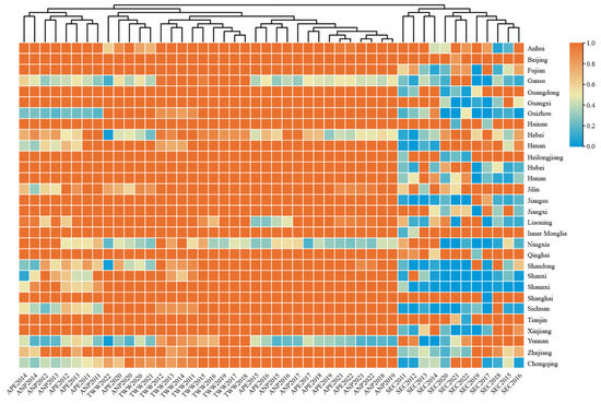
Figure 11.
Subindex efficiency clustering heatmap based on the Euclidean distance method.
The clustering results further reveal important relationships among the indicators. In particular, TWW, ANP, and APE exhibit a high degree of correlation, underscoring their shared linkage through pollution control and environmental management in the first stage. By contrast, these indicators are weakly correlated with sudden environmental change events, indicating that such events are more influenced by stochastic external factors than by structural pollution constraints. These findings highlight that while pollution-related undesirable outputs tend to evolve in a coordinated manner, climate and disaster-related indicators are driven by distinct mechanisms, reinforcing the need for differentiated governance strategies.
4.4. Robustness Check
This study employed the bootstrap DEA method to conduct a robustness check, with a resampling size of 720 and a 95% confidence interval. The comparison between the results of the bootstrap DEA method and those of the original network DEA model is presented in Figure 12 below. The comparative analysis indicates that although the efficiency values calculated using the bootstrap DEA method are generally lower than those obtained from the network DEA model, the overall variation trend remains consistent.
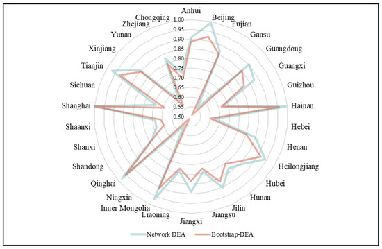
Figure 12.
Comparison of provincial ecological comprehensive efficiency between network DEA and bootstrap DEA.
According to Xue et al. (2021) [63], the bootstrap DEA method can address bias issues in small-sample settings, which explains why its estimated efficiency values are slightly lower than those of other DEA approaches. In summary, these results confirm the robustness of the methodological framework adopted in this study.
4.5. Driving Mechanism Analysis
Hierarchical heterogeneity reflects the intrinsic nature of geographical elements. Exploring its spatiotemporal attributes can reveal the evolutionary process of comprehensive ecological efficiency and its underlying formation mechanisms. This study has previously elaborated on the spatial heterogeneity of China’s comprehensive ecological efficiency and the potential influencing factors. Now, it further applies the geographical detector to verify and analyze the driving factors of the spatial differentiation of China’s comprehensive ecological efficiency, and further explores the interaction effects among different driving factors.
4.5.1. Risk Detector
The risk detector revealed differences between the gradations within each driving factor. We select six driving factors, namely ecological quality (EQ), industrial upgrading (IU), population size (PS), urban expansion (UE), infrastructure level (IL), and environmental protection (EP) efforts, whose spatial distributions are shown in Figure 13. The measurement methods for each factor are as follows: ecological quality is measured by the regional forest coverage rate; industrial upgrading is measured by the ratio of the added value of regional secondary and tertiary industries to GDP; population size is measured by the number of regional permanent residents; urban expansion is measured by the ratio of the regional urban area to the total land area. It should be noted that the “urban area” here is not equal to the “built-up area”, as urban areas generally include undeveloped areas. Infrastructure level is measured by the regional road network density, and environmental protection efforts are measured by the regional local government’s fiscal expenditure on environmental protection.
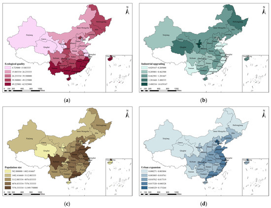
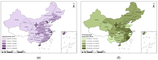
Figure 13.
The detection results for each driving factor: (a) ecological quality; (b) industrial upgrading; (c) population size; (d) urban expansion; (e) infrastructure level; and (f) environmental protection efforts.
In the analysis using Geodetector, the above six sets of data were sampled as independent variables, namely X1 (ecological quality), X2 (industrial upgrading), X3 (population size), X4 (urban expansion), X5 (infrastructure level), and X6 (environmental protection efforts), while the ecological comprehensive efficiency was treated as the dependent variable Y. The data were input into Geodetector in the form of (Y, X) to obtain the detection results of each driving factor. The results show that there are differences within each driving factor, and their explanatory power for the spatially stratified heterogeneity of China’s ecological comprehensive efficiency varies.
4.5.2. Factor Detector
Table 4 presents the explanatory power of each driving factor for China’s ecological comprehensive efficiency. The ranking of factors explaining the spatial differentiation of ecological comprehensive efficiency is as follows: X1 (ecological quality: 0.0204) > X6 (environmental protection efforts: 0.0197) > X3 (population size: 0.0180) > X5 (infrastructure level: 0.0166) > X4 (urban expansion: 0.0146) > X6 (industrial upgrading: 0.0046). The results indicate that ecological quality exerts the greatest influence on the spatial differentiation of ecological comprehensive efficiency, while environmental protection efforts and population sizes also show strong explanatory power. In contrast, urban expansion and industrial upgrading demonstrate relatively weaker effects.

Table 4.
The driving factor interprets the force probe results.
4.5.3. Interaction Detector
As indicated in Figure 14, the interaction between two driving factors exerts a more significant impact on China’s ecological comprehensive efficiency than a single driving factor acting independently, and this interaction manifests as a two-factor enhancement effect. It is evident from Figure 14 that, at the national scale, the dominant interactive driving factor combinations are population size ∩ environmental protection efforts, ecological quality ∩ environmental protection efforts, and urban expansion ∩ environmental protection efforts. When examined by region, we have the following:
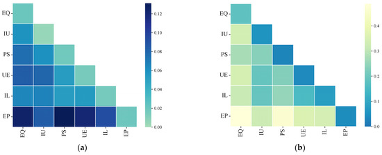
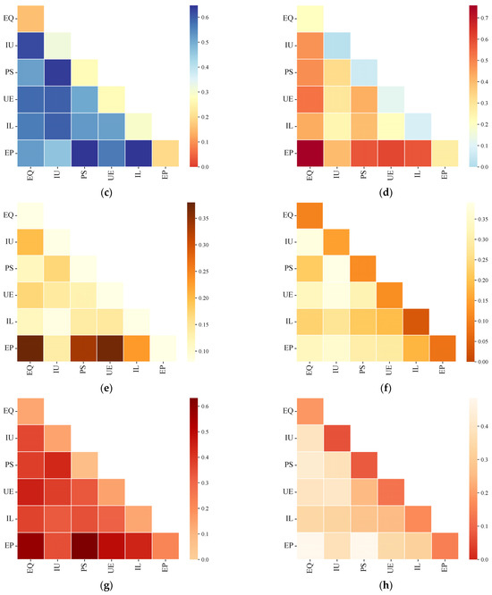
Figure 14.
Driver interaction probe results: (a) Whole China; (b) Northeast China; (c) Central China; (d) Northeast China; (e) East China; (f) South China; (g) North China; and (h) Southwest China.
1. The dominant interactive driving factor combinations in Central China are, in sequence, population size ∩ environmental protection efforts, infrastructure level ∩ environmental protection efforts, and ecological quality ∩ industrial upgrading.
2. In East China, the dominant interactive driving factor combinations are, in sequence, ecological quality ∩ environmental protection efforts, population size ∩ environmental protection efforts, and urban expansion ∩ environmental protection efforts.
3. The dominant interactive driving factor combinations in North China include, in sequence, population size ∩ environmental protection efforts, ecological quality ∩ environmental protection efforts, and urban expansion ∩ environmental protection efforts.
4. In Northeast China, the dominant interactive driving factor combinations are, in sequence, ecological quality ∩ environmental protection efforts, urban expansion ∩ environmental protection efforts, and population size ∩ environmental protection efforts.
5. The dominant interactive driving factor combinations in Northwest China are, in sequence, ecological quality ∩ environmental protection efforts, population size ∩ environmental protection efforts, and urban expansion ∩ environmental protection efforts.
6. In South China, the dominant interactive driving factor combinations are, in sequence, industrial upgrading ∩ population size, industrial upgrading ∩ urban expansion, and industrial upgrading ∩ ecological quality.
7. The dominant interactive driving factor combinations in Southwest China are, in sequence, ecological quality ∩ environmental protection efforts, population size ∩ environmental protection efforts, and ecological quality ∩ population size.
In general, while variations exist in the interactive driving factors influencing ecological comprehensive efficiency across China and its respective regions, these factors primarily revolve around four core dimensions, as follows: environmental protection efforts, population size, ecological quality, and urban expansion.
5. Discussion
This study provides a comprehensive assessment of China’s ecological comprehensive efficiency from 2011 to 2022 by integrating the water–energy–food system with climate change processes using a dynamic two-stage network SBM-DEA model. The findings reveal that national ecological efficiency remained moderate, with South China consistently leading and Northwest and Southwest provinces lagging. The W-E-F integration stage exhibited relatively high efficiency, whereas the climate change stage showed moderate efficiency with greater temporal fluctuations. These results align with prior studies by Simpson and Jewitt (2019) [5] and Mahmood et al. (2022) [6], highlighting the critical role of integrated resource management in improving system resilience, yet extend the literature by quantitatively linking efficiency dynamics to climate-induced variability, a connection often overlooked in previous research.
Hierarchical cluster analysis of the sub-indicators for undesirable outputs further reveals that there is a certain degree of synergy in the efficiency related to total wastewater, air pollutant emissions, and agricultural pollution, while the efficiency associated with sudden environmental change events shows a trend of high volatility and weak correlation with other traditional pollutants. This observation is consistent with the studies by Zhang et al. (2018) [10] and Kenway et al. (2011) [11], who pointed out that human activities and climate change simultaneously impact the ecological environment; however, the results of our study provide additional empirical evidence, demonstrating how these negative ecological factors interact with the water–energy–food (W-E-F) system and, together with climate change phenomena through the carbon linkage, exert a combined impact on the overall regional ecological efficiency. Furthermore, the finding that there is a strong correlation between the undesirable outputs of the three subsystems (water, energy, and food) in the W-E-F system echoes the call by Isaacs et al. (2016) [8] and Yue et al. (2021) [9]—that more comprehensive, system-wide approaches are needed to mitigate the damage caused by human activities to the ecological environment, rather than relying solely on intervention measures targeting specific sectors.
Geographical detector analysis shows that environmental protection efforts and ecological quality are the dominant driving factors, and their interaction has significantly intensified the spatial heterogeneity of ecological comprehensive efficiency across different regions. This supplements previous nationwide studies in China by Tian et al. (2025) [52] and Cao et al. (2025) [53], who adopted data envelopment analysis (DEA) and the geographical detector model in the water–energy–food (W-E-F) assessment. Moreover, our study further clarifies the spatial differences among various driving factors by demonstrating that these interactions exhibit spatial variations across China’s seven geographical regions, implying that targeted policy interventions may be more effective at improving efficiency.
Beyond the national context, it is also useful to compare China’s ecological efficiency patterns with those observed in other developing countries. For instance, cross-country DEA studies reveal that many South Asian economies face persistent inefficiency in the water–energy subsystem due to limited infrastructure and reliance on fossil fuels, while several Latin American countries exhibit relatively higher food system efficiency but weaker coordination across energy and water sectors (Franz et al., 2018 [25]; Ramanathan, 2002 [21]). Compared with these cases, China demonstrates stronger overall resource integration but suffers from pronounced regional disparities, especially between South and Northwest provinces. This indicates that although economic development and policy interventions have enabled China’s comprehensive ecological efficiency to perform exceptionally well among developing countries, the challenge of reducing interregional heterogeneity remains more severe. Therefore, while pursuing region-specific ecological improvement solutions, other developing countries should also ensure the coordinated development of various regions within their borders.
Furthermore, the proposed dynamic two-stage DEA–Geodetector framework is not limited to the Chinese context but can be adapted to other developing and developed regions. The general structure, which separates the W-E-F integration stage from the climate change stage, with CO2 emissions as the linking indicator, provides a flexible analytical pathway for assessing ecological efficiency under different environmental and institutional settings. In practice, adaptation requires two main types of adjustments. First, the indicator system should be tailored to local resource endowments and data availability. For example, in water-scarce regions of Sub-Saharan Africa [64], irrigation efficiency and groundwater use may serve as core inputs, while in Latin America, agricultural land expansion and biodiversity loss might be more relevant outputs [65]. Second, the policy and governance dimension must reflect regional realities [66]. While China emphasizes ecological civilization policies [67], other countries may frame interventions through climate adaptation strategies, sustainable agriculture programs, or renewable energy promotion [68]. These adjustments allow the framework to capture heterogeneous drivers while maintaining comparability across regions, thereby enhancing its value as a tool for international ecological governance research.
Overall, this study contributes to the literature in three main ways, as follows: first, by integrating the W-E-F nexus with climate change to assess ecological efficiency dynamically; second, by quantifying the interdependence of sub-indicators and identifying systemic feedback; and third, by demonstrating the amplified effects of interactive socioeconomic and infrastructure factors. In addition, by placing China’s experience in comparative perspective with other developing countries and clarifying the adaptability of the proposed framework, this study highlights both China’s relative advantages in resource integration and its persistent regional disparities. These findings provide actionable insights for policymakers to implement cross-regional coordination, phase-specific interventions, and synergistic management of both high- and low-performing indicators, ultimately promoting sustainable ecological governance in China and offering methodological references for other regions worldwide.
6. Conclusions and Suggestions
6.1. Conclusions
Based on provincial panel data from 2011 to 2022, the following conclusions are drawn:
1. Overall performance: From 2011 to 2022, China’s ecological comprehensive efficiency showed significant regional disparities, with an overall good performance (average value of 0.8179), with South China leading and Southwest lagging, and interregional differences identified as the dominant source of efficiency gaps.
2. Stage differences: During the water–energy–food integration stage (S1), China’s stage efficiency was generally high (average of 0.8712), with South China leading, and Northwest and Southwest lagging. During the climate change stage (S2), stage efficiency was moderate (average of 0.4360), with South China remaining the most efficient, and the Southwest performing the worst.
3. Sub-variable efficiency: From 2011 to 2022, TWW, ANP, and APE exhibited a high degree of correlation, underscoring their shared linkage through pollution control and environmental management. By contrast, these indicators were weakly correlated with sudden environmental change events, indicating that such events are more influenced by stochastic external factors than by structural pollution constraints.
4. Driving mechanisms: From 2011 to 2022, ecological quality exerted the greatest influence on the spatial differentiation of ecological comprehensive efficiency. In contrast, urban expansion and industrial upgrading demonstrated relatively weaker effects. Variations exist in the interactive driving factors influencing ecological comprehensive efficiency across China and its respective regions, highlighting four core dimensions, as follows: environmental protection efforts, population size, ecological quality, and urban expansion, as central to regional efficiency patterns.
Finally, the methodological integration of the dynamic two-stage DEA and Geodetector developed in this study also provides valuable guidance for international climate governance. By offering a transparent efficiency metric and identifying heterogeneous drivers, this framework enables cross-country comparisons, supports the equitable allocation of emission reduction responsibilities under the principle of common but differentiated responsibilities (CBDRs) [69], and informs the design of region-specific yet coordinated policies. In this sense, the framework contributes not only to advancing academic research but also to providing practical tools for global climate governance, carbon trading mechanisms, and progress monitoring toward the Sustainable Development Goals.
In practical terms, the findings of this study also demonstrate clear application potential. For instance, addressing the persistent efficiency gap between South and Northwest China provides a scientific basis for targeted regional coordination projects such as water diversion and ecological compensation. The importance of energy-related efficiency suggests that expanding renewable energy deployment and piloting green electricity trading can effectively enhance ecological outcomes. Similarly, the role of agricultural non-point source pollution points to the value of precision agriculture and fertilizer reduction programs as concrete measures to reduce emissions while sustaining food security. These examples illustrate how the empirical results can be translated into actionable policies, thereby enhancing the practical significance of this research.
6.2. Limitations
This study uses provincial panel data from China covering 2011 to 2022 to analyze the ecological comprehensive efficiency and its driving factors. Due to the time lag in the acquisition of statistical data, data for the latest year is currently unavailable. In addition, the analysis is limited to the national macro level; future research should focus on the micro-city level, explore the characteristics of different urban attributes, and incorporate comparative analyses with the environmental effects of other developing countries to reveal a more comprehensive heterogeneity of results. Moreover, subsequent studies may attempt to construct an ecological comprehensive efficiency indicator system with three separate subsystems (water, energy, and food) based on the parallel DEA method, to further explore how different subsystems affect ecological efficiency and their heterogeneous influencing factors.
Methodologically, the dynamic two-stage DEA model assumes a stable production frontier, which may not fully capture abrupt policy shifts or nonlinear impacts of extreme climate events. Similarly, while the Geodetector is effective at detecting spatial heterogeneity and interaction effects, it cannot establish causal mechanisms. The selection of climate indicators, though balanced between natural variability and anthropogenic drivers, remains limited—annual averages of temperature and precipitation may obscure local extremes, and the focus on CO2 excludes other important greenhouse gases such as methane and nitrous oxide. In addition, the study adopts the emission factor method to calculate CO2 emissions related to water conservancy and agriculture. Although the emission factor method is widely applied for rapid carbon accounting at the macro level due to its simplicity and low data requirements, it has inherent limitations, such as low accounting accuracy caused by spatiotemporal heterogeneity and the inability to effectively distinguish between direct and indirect emissions.
From a data perspective, reliance on provincial-level panel data may mask intra-provincial differences at the city or watershed scale, and the use of statistical yearbook data introduces potential reporting inconsistencies across provinces and years. Finally, the study period (2011–2022) does not reflect the most recent policy dynamics under China’s “dual carbon” strategy. These limitations should be addressed in future research by incorporating finer-scale, multi-source datasets, more comprehensive climate and socioeconomic indicators, and advanced methodological frameworks.
6.3. Suggestions
To enhance ecological comprehensive efficiency and promote sustainable regional development, the following policy implications are proposed:
1. Focus on regional disparities and establish cross-regional coordination mechanisms to narrow efficiency gaps. In response to the regional differentiation of “South China leading, Northwest lagging” and the finding that interregional overlap is the main source of efficiency gaps, a twofold approach is recommended. First, a “South China–Northwest/Southwest” pairing assistance mechanism should be established to enable high-efficiency provinces to transfer ecological governance experience, technologies, and funding to lagging regions, with priority on enhancing the foundational capacities of ecologically vulnerable areas in the Northwest and low-efficiency regions in the Southwest. Second, for provinces with relatively low national total efficiency, differentiated improvement plans should be formulated based on their resource endowments to reduce efficiency losses caused by overlapping regional development.
2. Implement phase-specific policies and strengthen policy continuity. Considering that efficiency remained relatively high during S1 but lagged in the Southwest and Northwest, and remained moderate during S2, with clear effects of the 2015 ecological civilization policies, phase-specific strategies are required. During S1, South China’s advantages should be consolidated while providing the Southwest and Northwest regions with water–energy–food integration support (e.g., water-saving irrigation, coordinated clean energy supply) to resolve inefficiencies in resource allocation. During S2, ecological civilization policies initiated in 2015 should be continued and upgraded by expanding the influence of “stable high-efficiency clusters” through the promotion of climate adaptation technologies (e.g., carbon reduction, extreme weather response) to surrounding provinces, and by establishing a dynamic monitoring system for S2 efficiency to manage industrial pollution impacts and reduce the number of low-efficiency provinces.
3. Address indicator shortcomings, strengthen synergy of advantageous indicators, and resolve bottlenecks of low-efficiency indicators. First, the synergistic management of high-performing indicators should be reinforced by promoting integrated governance of “agricultural pollution–air pollution” (e.g., controlling fertilizer and pesticide volatilization, enhancing straw resource utilization) to prevent mutual exacerbation. Second, for the low efficiency of temperature change, targeted mitigation should focus on industrially polluted provinces through industrial structure optimization (reducing the share of high-energy-consuming and high-emission industries) and enhancing carbon sink capacity (increasing forest coverage) to buffer temperature fluctuations. Third, the post-2015 improvements in sudden environmental change efficiency should be consolidated by establishing a nationwide early warning platform for environmental emergencies to improve response speed.
4. Anchor core drivers, strengthen key factors, and activate interaction effects. Priority should be given to addressing infrastructure deficiencies in lagging regions by increasing road network density and upgrading environmental facilities (e.g., wastewater treatment plants, waste-to-energy plants) to directly enhance efficiency. Urban expansion should be regulated to avoid uncontrolled sprawl encroaching on ecological spaces; in rapidly urbanizing areas, a coordinated “ecological redline–urban planning” mechanism should be implemented to balance urbanization and ecological protection. Interaction effects among driving factors should be leveraged. Based on the dominant interaction combinations in the seven geographical regions, Central China should enhance coordinated investment in environmental protection expenditure and infrastructure construction, while South China should strengthen the synergy between ecological quality protection and industrial upgrading policies, thereby amplifying the driving effect through “1 + 1 > 2” interactions.
Author Contributions
Conceptualization, F.-R.R.; methodology, F.-R.R. and F.-Y.S.; validation, F.-R.R. and H.-L.L.; formal analysis, F.-Y.S., X.-Y.L. and H.-L.L.; investigation, F.-Y.S.; resources, F.-Y.S. and H.-L.L.; data curation, F.-Y.S.; writing—original draft preparation, F.-R.R.; writing—review and editing, F.-Y.S., X.-Y.L. and H.-L.L.; visualization, X.-Y.L. and H.-L.L.; supervision, X.-Y.L.; project administration, F.-R.R. and X.-Y.L.; funding acquisition, F.-R.R. All authors have read and agreed to the published version of the manuscript.
Funding
This research was funded by the National Social Science Foundation Project (grant number 24BJY142), the China Postdoctoral Science Foundation Project (grant number 2023M741632), and the Major Project of Philosophy and Social Science Research in Universities of Jiangsu Province (grant number 2022SJZD053).
Data Availability Statement
The original contributions presented in this study are included in the article. Further inquiries can be directed to the corresponding author.
Acknowledgments
We gratefully acknowledge the editor and reviewers for their insightful comments on earlier drafts of this paper. This research was funded by the National Social Science Foundation Project (grant number 24BJY142), the China Postdoctoral Science Foundation Project (grant number 2023M741632), and the Major Project of Philosophy and Social Science Research in Universities of Jiangsu Province (grant number 2022SJZD053).
Conflicts of Interest
The authors declare no conflicts of interest.
Appendix A
The figure below shows the study area of this research and its division into seven major regions based on economic and geographical characteristics.
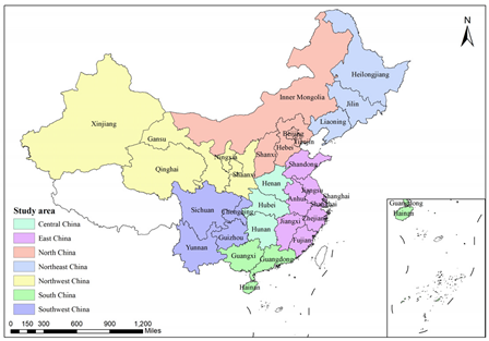
Appendix B
The agricultural non-point source pollution load in this study is defined as follows:
Among them, represents the agricultural non-point source pollution load; denotes the statistical data of pollution unit ; stands for the generation coefficient of pollution unit ; is the loss coefficient of pollution unit , which is determined by the pollution unit itself and the natural conditions of the region where the pollution unit is located.
This study selects the two most significant types of agricultural non-point source pollution in agricultural production and operation activities—chemical fertilizer application and livestock breeding—as the research objects of agricultural non-point source pollution. The original data of these two parts are all derived from the China Rural Statistical Yearbook, while the relevant coefficients were obtained from the Handbook of Chemical Fertilizer Loss Coefficients in China and the Table of Livestock Pollutant Generation Coefficients, published by the State Environmental Protection Administration of China.
Appendix C
The calculation formula for CO2 emissions from the water conservancy sector is as follows:
Among them, represents CO2 emissions from water conservancy, denotes the conversion coefficient of carbon emissions from standard coal, and stands for water conservancy-related energy consumption. Here, refers to regions, while represents processes such as water lifting, water treatment, and water supply. is the water resource volume of process , denotes the energy consumption coefficient of process , and stands for the conversion coefficient for converting electricity into standard coal. The relevant original data and conversion coefficients are derived from the China Water Conservancy Statistical Yearbook and the China Energy Statistical Yearbook.
Appendix D
Based on the classification in National Economic Industry Classification (GB/T 4754-2017) [70], the energy enterprises accounted for in this study belong to the following industries: mining support activities, coal mining and washing industry, oil and gas extraction industry, electric power and heat production and supply industry, gas production and supply industry, petroleum processing, coking and nuclear fuel processing industry.
Appendix E
The calculation formula for CO2 emissions from the agriculture sector is as follows:
Among them, represents agricultural carbon emissions, denotes the chemical fertilizer application amount, stands for the plastic film usage amount, is the agricultural diesel usage amount, represents the pesticide usage amount, is the crop sowing area, and denotes the irrigation area. The aforementioned original data are all derived from the China Rural Statistical Yearbook.
Meanwhile, , , , , , and μ, respectively, refer to the carbon emission coefficients of the six types of agricultural activities, which are obtained from the Chinese Life Cycle Database and the IPCC Fourth Assessment Report.
References
- Ahmed, H.; Rahul, T. Climate Changes through Data Science: Understanding and Mitigating Environmental Crisis. Mesopotamian J. Big Data 2023, 20, 125–137. [Google Scholar] [CrossRef]
- Che, S.; Wang, J.; Chen, H. Can China’s decentralized energy governance reduce carbon emissions? Evidence from new energy demonstration cities. Energy 2023, 284, 128665. [Google Scholar] [CrossRef]
- The Changing Landscape of Global Emissions—CO2 Emissions in 2023—Analysis. Available online: https://www.iea.org/reports/co2-emissions-in-2023/the-changing-landscape-of-global-emissions (accessed on 28 August 2025).
- Yoon, P.; Lee, S.; Choi, J.; Yoo, S.; Hur, S. Analysis of Climate Change Impact on Resource Intensity and Carbon Emissions in Protected Farming Systems Using Water-Energy-Food-Carbon Nexus. Resour. Conserv. Recycl. 2022, 184, 106394. [Google Scholar] [CrossRef]
- Simpson, G.; Jewitt, G. The Development of the Water-Energy-Food Nexus as a Framework for Achieving Resource Security: A Review. Front. Environ. Sci. 2019, 7, 8. [Google Scholar] [CrossRef]
- Mahmood, M.; Shahab, S.; Shahbaz, M. The Relevance of Economic Freedom for Energy, Environment, and Economic Growth in Asia-Pacific Region. Environ. Sci. Pollut. Res. 2022, 29, 5396–5405. [Google Scholar] [CrossRef]
- Mroue, A.; Mohtar, R.; Pistikopoulos, E.; Holtzapple, M. Energy Portfolio Assessment Tool (EPAT): Sustainable Energy Planning Using the WEF Nexus Approach—Texas Case. Sci. Total Environ. 2019, 648, 1649–1664. [Google Scholar] [CrossRef]
- Isaacs, K.; Snapp, S.; Chung, K.; Waldman, K. Assessing the Value of Diverse Cropping Systems under a New Agricultural Policy Environment in Rwanda. Food Sec. 2016, 8, 491–506. [Google Scholar] [CrossRef]
- Yue, Q.; Zhang, F.; Wang, Y.; Zhang, X.; Guo, P. Fuzzy Multi-Objective Modelling for Managing Water-Food-Energy-Climate Change-Land Nexus towards Sustainability. J. Hydrol. 2021, 596, 125704. [Google Scholar] [CrossRef]
- Zhang, C.; Chen, X.; Li, Y.; Ding, W.; Fu, G. Water-Energy-Food Nexus: Concepts, Questions and Methodologies. J. Clean. Prod. 2018, 195, 625–639. [Google Scholar] [CrossRef]
- Kenway, S.; Lant, P.; Priestley, T. Quantifying Water–Energy Links and Related Carbon Emissions in Cities. J. Water Clim. Change 2011, 2, 247–259. [Google Scholar] [CrossRef]
- Chamas, Z.; Abou Najm, M.; Al-Hindi, M.; Yassine, A.; Khattar, R. Sustainable Resource Optimization under Water-Energy-Food-Carbon Nexus. J. Clean. Prod. 2021, 278, 123894. [Google Scholar] [CrossRef]
- Li, M.; Cao, X.; Liu, D.; Fu, Q.; Li, T.; Shang, R. Sustainable Management of Agricultural Water and Land Resources under Changing Climate and Socio-Economic Conditions: A Multi-Dimensional Optimization Approach. Agric. Water Manag. 2022, 259, 107235. [Google Scholar] [CrossRef]
- Horton, D.; Johnson, N.; Singh, D.; Swain, D.; Rajaratnam, B.; Diffenbaugh, N. Contribution of Changes in Atmospheric Circulation Patterns to Extreme Temperature Trends. Nature 2015, 522, 465–469. [Google Scholar] [CrossRef]
- Angélil, O.; Stone, D.; Wehner, M.; Paciorek, C.; Krishnan, H.; Collins, W. An Independent Assessment of Anthropogenic Attribution Statements for Recent Extreme Temperature and Rainfall Events. J. Clim. 2017, 30, 5–16. [Google Scholar] [CrossRef]
- Chapman, S.; Watson, J.; Salazar, A.; Thatcher, M.; McAlpine, C. The Impact of Urbanization and Climate Change on Urban Temperatures: A Systematic Review. Landsc. Ecol. 2017, 32, 1921–1935. [Google Scholar] [CrossRef]
- Sun, Y.; Zhang, X.; Ren, G.; Zwiers, F.; Hu, T. Contribution of Urbanization to Warming in China. Nat. Clim. Change 2016, 6, 706–709. [Google Scholar] [CrossRef]
- Yu, R.; Zhai, P.; Lu, Y. Implications of Differential Effects between 1.5 and 2 °C Global Warming on Temperature and Precipitation Extremes in China’s Urban Agglomerations. Int. J. Climatol. 2018, 38, 2374–2385. [Google Scholar] [CrossRef]
- Fu, T.; Tian, H. Climate Change Penalty to Ozone Air Quality: Review of Current Understandings and Knowledge Gaps. Curr. Pollut. Rep. 2019, 5, 159–171. [Google Scholar] [CrossRef]
- Han, W.; Li, Z.; Wu, F.; Zhang, Y.; Guo, J.; Su, T.; Cribb, M.; Fan, J.; Chen, T.; Wei, J.; et al. The Mechanisms and Seasonal Differences of the Impact of Aerosols on Daytime Surface Urban Heat Island Effect. Atmos. Chem. Phys. 2020, 20, 6479–6493. [Google Scholar] [CrossRef]
- Ramanathan, R. Combining Indicators of Energy Consumption and CO2 Emissions: A Cross-Country Comparison. Int. J. Glob. Energy Issues 2002, 17, 214–227. [Google Scholar] [CrossRef]
- Feng, C.; Chu, F.; Ding, J.; Bi, G.; Liang, L. Carbon Emissions Abatement (CEA) Allocation and Compensation Schemes Based on DEA. Omega 2015, 53, 78–89. [Google Scholar] [CrossRef]
- Wu, J.; Chu, J.; Liang, L. Target Setting and Allocation of Carbon Emissions Abatement Based on DEA and Closest Target: An Application to 20 APEC Economies. Nat. Hazards 2016, 84, 279–296. [Google Scholar] [CrossRef]
- Yan, X.; Fang, L.; Mu, L. How Does the Water-Energy-Food Nexus Work in Developing Countries? An Empirical Study of China. Sci. Total Environ. 2020, 716, 134791. [Google Scholar] [CrossRef] [PubMed]
- Franz, M.; Schlitz, N.; Schumacher, K. Globalization and the Water-Energy-Food Nexus—Using the Global Production Networks Approach to Analyze Society-Environment Relations. Environ. Sci. Policy 2018, 90, 201–212. [Google Scholar] [CrossRef]
- Han, X.; Hua, E.; Engel, B.; Guan, J.; Yin, J.; Wu, N.; Sun, S.; Wang, Y. Understanding Implications of Climate Change and Socio-Economic Development for the Water-Energy-Food Nexus: A Meta-Regression Analysis. Agric. Water Manag. 2022, 269, 107693. [Google Scholar] [CrossRef]
- Deng, G.; Jiang, H.; Ma, S.; Wen, Y.; He, C.; Sheng, L.; Gu, D. How Water–Energy–Food Services and Their Interactions Change along Multiple Environmental Gradients. Agric. Water Manag. 2025, 309, 109339. [Google Scholar] [CrossRef]
- Wolde, Z.; Wei, W.; Likessa, D.; Omari, R.; Ketema, H. Understanding the Impact of Land Use and Land Cover Change on Water–Energy–Food Nexus in the Gidabo Watershed, East African Rift Valley. Nat. Resour. Res. 2021, 30, 2687–2702. [Google Scholar] [CrossRef]
- Taniguchi, M.; Masuhara, N.; Teramoto, S. Tradeoffs in the Water-Energy-Food Nexus in the Urbanizing Asia-Pacific Region. Water Int. 2018, 43, 892–903. [Google Scholar] [CrossRef]
- Yu, Y.; Zhang, C.; Zhu, W.; Park, S.; Shi, Q. Identifying the Driving Factors of Water Consumption from Water-Energy-Food Nexus in the Yangtze River Delta Region, China. Environ. Sci. Pollut. Res. 2021, 28, 48638–48655. [Google Scholar] [CrossRef]
- Li, G.; Huang, D.; Sun, C.; Li, Y. Developing Interpretive Structural Modeling Based on Factor Analysis for the Water-Energy-Food Nexus Conundrum. Sci. Total Environ. 2019, 651, 309–322. [Google Scholar] [CrossRef]
- Jin, B.; Shi, R.; Chen, S.; He, Y.; Zhao, M. Analysis of the Factors Influencing the Water-Energy-Food System Stress in China. Environ. Sci. Pollut. Res. 2023, 31, 46686–46702. [Google Scholar] [CrossRef]
- Qin, Q.; He, W.; Yuan, L.; Degefu, D.; Ramsey, T. Coupled and Coordinated Development of Water-Energy-Food-Ecology-Land System in the Yangtze River Delta, China. npj Clean Water 2025, 8, 38. [Google Scholar] [CrossRef]
- Ling, M.; Qi, T.; Li, W.; Yu, L.; Xia, Q. Simulating and Predicting the Development Trends of the Water–Energy–Food–Ecology System in Henan Province, China. Ecol. Indic. 2024, 158, 111513. [Google Scholar] [CrossRef]
- Zhang, T.; Tan, Q.; Yu, X.; Zhang, S. Synergy Assessment and Optimization for Water-Energy-Food Nexus: Modeling and Application. Renew. Sustain. Energy Rev. 2020, 134, 110059. [Google Scholar] [CrossRef]
- David, L.; Adepoju, O.; Nwulu, N.; Aigbavboa, C. Determining the Impact of Economic Indicators on Water, Energy and Food Nexus for Sustainable Resource Security. Clean Techn. Environ. Policy 2024, 26, 803–820. [Google Scholar] [CrossRef]
- Wu, L.; Elshorbagy, A.; Alam, M. Dynamics of Water-Energy-Food Nexus Interactions with Climate Change and Policy Options. Environ. Res. Commun. 2022, 4, 015009. [Google Scholar] [CrossRef]
- Mooren, C.; Munaretto, S.; La Jeunesse, I.; Sievers, E.; Hegger, D.; Driessen, P.; Hüesker, F.; Cirelli, C.; Canovas, I.; Mounir, K.; et al. Water–Energy–Food–Ecosystem Nexus: How to Frame and How to Govern. Sustain. Sci. 2025. [Google Scholar] [CrossRef]
- Zhang, T.; Xu, Y. Evaluation on the Efficiency of Water-Energy-Food Nexus Based on Data Envelopment Analysis (DEA) and Malmquist in Different Regions of China. Int. J. Comput. Intell. Syst. 2019, 12, 1649. [Google Scholar] [CrossRef]
- Li, J.; Liu, S.; Zhao, Y.; Gong, Z.; Wei, G.; Wang, L. Water-Energy-Food Nexus and Eco-Sustainability: A Three-Stage Dual-Boundary Network DEA Model for Evaluating Jiangsu Province in China. Int. J. Comput. Intell. Syst. 2021, 14, 1501. [Google Scholar] [CrossRef]
- Han, D.; Yu, D.; Cao, Q. Assessment on the Features of Coupling Interaction of the Food-Energy-Water Nexus in China. J. Clean. Prod. 2020, 249, 119379. [Google Scholar] [CrossRef]
- Lins, M.; Gomes, E.; Soares de Mello, J.; Soares de Mello, A. Olympic Ranking Based on a Zero Sum Gains DEA Model. Eur. J. Oper. Res. 2003, 148, 312–322. [Google Scholar] [CrossRef]
- Yang, M.; Hou, Y.; Ji, Q.; Zhang, D. Assessment and Optimization of Provincial CO2 Emission Reduction Scheme in China: An Improved ZSG-DEA Approach. Energy Econ. 2020, 91, 104931. [Google Scholar] [CrossRef]
- Chu, J.; Wu, J.; Song, M. An SBM-DEA Model with Parallel Computing Design for Environmental Efficiency Evaluation in the Big Data Context: A Transportation System Application. Ann. Oper. Res. 2018, 270, 105–124. [Google Scholar] [CrossRef]
- Huang, D.; Shen, Z.; Sun, C.; Li, G. Shifting from Production-Based to Consumption-Based Nexus Governance: Evidence from an Input–Output Analysis of the Local Water-Energy-Food Nexus. Water Resour. Manag. 2021, 35, 1673–1688. [Google Scholar] [CrossRef]
- Yeh, T.; Chen, T.; Lai, P. A Comparative Study of Energy Utilization Efficiency between Taiwan and China. Energy Policy 2010, 38, 2386–2394. [Google Scholar] [CrossRef]
- Zhou, P.; Ang, B.; Wang, H. Energy and CO2 Emission Performance in Electricity Generation: A Non-Radial Directional Distance Function Approach. Eur. J. Oper. Res. 2012, 221, 625–635. [Google Scholar] [CrossRef]
- Zhang, N.; Choi, Y. Total-Factor Carbon Emission Performance of Fossil Fuel Power Plants in China: A Metafrontier Non-Radial Malmquist Index Analysis. Energy Econ. 2013, 40, 549–559. [Google Scholar] [CrossRef]
- Wu, F.; Fan, L.W.; Zhou, P.; Zhou, D. Industrial Energy Efficiency with CO2 Emissions in China: A Nonparametric Analysis. Energy Policy 2012, 49, 164–172. [Google Scholar] [CrossRef]
- Sueyoshi, T.; Yuan, Y. Measuring Energy Usage and Sustainability Development in Asian Nations by DEA Intermediate Approach. Econ. Struct. 2018, 7, 6. [Google Scholar] [CrossRef]
- Zhang, Y.; Yu, Z.; Zhang, J. Analysis of Carbon Emission Performance and Regional Differences in China’s Eight Economic Regions: Based on the Super-Efficiency SBM Model and the Theil Index. PLoS ONE 2021, 16, e0250994. [Google Scholar] [CrossRef]
- Tian, G.; Li, J.; Wu, Z.; Zhao, Q.; Xia, Q.; Zhang, J.; Niu, X. Unveiling the Resilience of the Water-Energy-Food Nexus: A Context-Specific Framework and Evolutionary Insights for the Yellow River Basin. Agric. Water Manag. 2025, 315, 109514. [Google Scholar] [CrossRef]
- Cao, X.; Li, X.; Zhou, Y. Unveiling the Driving Mechanisms of the Network Land Use Efficiency: A Multi-Model Research. Stoch Environ Res. Risk Assess 2025, 39, 3853–3873. [Google Scholar] [CrossRef]
- Zhang, S.; Yang, D.; Meng, H.; Wan, M.; Ji, Y.; Zhang, J.; Yang, H. Spatiotemporal Pattern Evolution and Driving Factors of China’s Energy Transition from a Heterogeneity Perspective. J. Clean. Prod. 2025, 487, 144624. [Google Scholar] [CrossRef]
- Jiang, L.; Liu, S.; Liu, L.; Liu, C. Revealing the Spatiotemporal Characteristics and Drivers of the Block-Scale Thermal Environment near a Large River: Evidences from Shanghai, China. Build. Environ. 2022, 226, 109728. [Google Scholar] [CrossRef]
- Li, Y.; Xie, W.; Zhang, J.; Zhang, D. Spatiotemporal Changes and Driving Factors of Ecological Environmental Quality in the Yongding-Luan River Basin Based on RSEI. Front. Environ. Sci. 2024, 12, 1494098. [Google Scholar] [CrossRef]
- Zhang, T.; Tan, Q.; Cai, Y. General Equilibrium Analysis of Carbon Tax Policy on Water-Energy-Food Nexus Efficiency. Energy 2024, 304, 132079. [Google Scholar] [CrossRef]
- Chen, Y.; Liu, L. Improving Eco-Efficiency in Coal Mining Area for Sustainability Development: An Emergy and Super-Efficiency SBM-DEA with Undesirable Output. J. Clean. Prod. 2022, 339, 130701. [Google Scholar] [CrossRef]
- Sun, Y.; Zhao, T.; Xia, L. Spatial-Temporal Differentiation of Carbon Efficiency and Coupling Coordination Degree of Chinese County Territory and Obstacles Analysis. Sustain. Cities Soc. 2022, 76, 103429. [Google Scholar] [CrossRef]
- Lee, C.C.; He, Z.W.; Luo, H.P. Spatio-Temporal Characteristics of Land Ecological Security and Analysis of Influencing Factors in Cities of Major Grain-Producing Regions of China. Environ. Impact Assess. Rev. 2024, 104, 107344. [Google Scholar] [CrossRef]
- Lu, L.; Chiu, S.; Chiu, Y.; Chang, T. Sustainability Efficiency of Climate Change and Global Disasters Based on Greenhouse Gas Emissions from the Parallel Production Sectors—A Modified Dynamic Parallel Three-Stage Network DEA Model. J. Environ. Manag. 2022, 317, 115401. [Google Scholar] [CrossRef]
- Tone, K. A Slacks-Based Measure of Efficiency in Data Envelopment Analysis. Eur. J. Oper. Res. 2001, 130, 498–509. [Google Scholar] [CrossRef]
- Xue, L.; Zhang, W.; Zheng, Z. Measurement and influential factors of the efficiency of coal resources of China’s provinces: Based on Bootstrap-DEA and Tobit. Energy 2021, 221, 119763. [Google Scholar] [CrossRef]
- Beliyou, H.; Dawit, M.; Jowel, C. Hierarchical Modelling of Small-Scale Irrigation: Constraints and Opportunities for Adoption in Sub-Saharan Africa. Water Econ. Policy 2022, 8, 2250005. [Google Scholar] [CrossRef]
- Que, Y.; Zhang, J.; Qin, R. Analysis on the loss path and cooperative protection of global biodiversity based on input-output model. J. Clean. Prod. 2023, 419, 138232. [Google Scholar] [CrossRef]
- Niu, B.; Ge, D.; Sun, J. Multi-scales urban-rural integrated development and land-use transition: The story of China. Habitat Int. 2023, 132, 102744. [Google Scholar] [CrossRef]
- Weins, N.; Zhu, A.; Qian, J. Ecological Civilization in the making: The ‘construction’ of China’s climate-forestry nexus. Environ. Sociol. 2023, 9, 6–19. [Google Scholar] [CrossRef]
- Ahmad, B.; Dalia, S. Renewable Energy and Sustainable Agriculture: Review of Indicators. Sustainability 2023, 15, 14307. [Google Scholar] [CrossRef]
- Zheng, Z. Re-calculation of responsibility distribution and spatiotemporal patterns of global production carbon emissions from the perspective of global value chain. Sci. Total Environ. 2021, 773, 145065. [Google Scholar] [CrossRef]
- GB/T 4754-2017; Industrial Classification for National Economic Activities. General Administration of Quality Supervision, Inspection and Quarantine of the People’s Republic of China: Beijing, China; Standardization Administration of China: Beijing, China, 2017. Available online: https://openstd.samr.gov.cn/bzgk/gb/newGbInfo?hcno=A703F0E23DD165A5A1318679F312D158 (accessed on 9 October 2025).
Disclaimer/Publisher’s Note: The statements, opinions and data contained in all publications are solely those of the individual author(s) and contributor(s) and not of MDPI and/or the editor(s). MDPI and/or the editor(s) disclaim responsibility for any injury to people or property resulting from any ideas, methods, instructions or products referred to in the content. |
© 2025 by the authors. Licensee MDPI, Basel, Switzerland. This article is an open access article distributed under the terms and conditions of the Creative Commons Attribution (CC BY) license (https://creativecommons.org/licenses/by/4.0/).