Article

Comparative Analysis of Deep Learning and Traditional Methods for High-Resolution Cropland Extraction with Different Training Data Characteristics

1
National Supercomputing Center in Zhengzhou, Zhengzhou University, Zhengzhou 450001, China
2
Institute of Remote Sensing Science and Engineering, Faculty of Geographical Sciences, Beijing Normal University, Beijing 100875, China
3
School of Water Conservancy and Transportation, Zhengzhou University, Zhengzhou 450001, China
4
State Key Laboratory of Remote Sensing Science, Beijing Normal University, Beijing 100875, China
5
The 27th Research Institute of China Electronics Technology Group Corporation, Zhengzhou 450047, China
6
Henan Key Laboratory of Remote Sensing of Ecological Environment, Zhengzhou 450047, China
7
School of Geoscience and Technology, Zhengzhou University, Zhengzhou 450001, China
*
Authors to whom correspondence should be addressed.
Land 2025, 14(10), 2038; https://doi.org/10.3390/land14102038
Submission received: 29 August 2025 / Revised: 8 October 2025 / Accepted: 9 October 2025 / Published: 13 October 2025

Abstract

High-resolution remote sensing (HRRS) imagery enables the extraction of cropland information with high levels of detail, especially when combined with the impressive performance of deep convolutional neural networks (DCNNs) in understanding these images. Comprehending the factors influencing DCNNs’ performance in HRRS cropland extraction is of considerable importance for practical agricultural monitoring applications. This study investigates the impact of classifier selection and different training data characteristics on the HRRS cropland classification outcomes. Specifically, Gaofen-1 composite images with 2 m spatial resolution are employed for HRRS cropland extraction, and two county-wide regions with distinct agricultural landscapes in Shandong Province, China, are selected as the study areas. The performance of two deep learning (DL) algorithms (UNet and DeepLabv3+) and a traditional classification algorithm, Object-Based Image Analysis with Random Forest (OBIA-RF), is compared. Additionally, the effects of different band combinations, crop growth stages, and class mislabeling on the classification accuracy are evaluated. The results demonstrated that the UNet and DeepLabv3+ models outperformed OBIA-RF in both simple and complex agricultural landscapes, and were insensitive to the changes in band combinations, indicating their ability to learn abstract features and contextual semantic information for HRRS cropland extraction. Moreover, compared with the DL models, OBIA-RF was more sensitive to changes in the temporal characteristics. The performance of all three models was unaffected when the mislabeling error ratio remained below 5%. Beyond this threshold, the performance of all models decreased, with UNet and DeepLabv3+ showing similar performance decline trends and OBIA-RF suffering a more drastic reduction. Furthermore, the DL models exhibited relatively low sensitivity to the patch size of sample blocks and data augmentation. These findings can facilitate the design of operational implementations for practical applications.

1. Introduction

Mapping cropland in a timely and dependable manner is crucial for a multitude of agricultural applications, including periodic crop condition monitoring, agricultural resource assessment and sustainable agricultural practices [1,2,3]. The rapid development of remote sensing (RS) technologies has facilitated the acquisition of large amounts of high spatial-resolution imagery, offering detailed information about the land surface and enabling the development of techniques specifically for the precise extraction of cropland areas. Although this abundance of data offers unprecedented opportunities for precise cropland extraction, it also poses considerable challenges. The rich information of high-resolution imagery hinders the traditional classification methods from effectively extracting robust cropland features and achieving satisfactory classification accuracy. This gap between data availability and processing capability highlights the urgent need for advanced approaches to fully exploit the potential of high-resolution RS data in cropland extraction.
Deep learning (DL) algorithms, and, in particular, deep convolutional neural networks (DCNNs) [4], can automatically learn abstract features with strong generalization and transferability. They have been increasingly drawing attention in the RS big data analysis [5,6,7] and have been widely applied to challenging issues associated with the interpretation of high-resolution remote sensing (HRRS) imagery, such as object detection [8,9], land cover/use classification [10,11], and cropland mapping [12,13,14]. DCNNs’ effectiveness has made them an attractive and robust alternative for HRRS cropland mapping.
DL algorithms have substantially enhanced classification performance, and extensive studies have established the superiority of DCNNs over traditional classifiers [12,15]. However, selecting a suitable network architecture is paramount when applying DL algorithms to high-resolution cropland mapping. The UNet [16] and Deeplabv3+ [17] architectures, with their robust generalization capabilities, are frequently employed in RS classifications [18,19,20,21]. For example, Zhang et al. [22] introduced a knowledge-driven cross-scale sample transfer approach and employed DeepLabv3+ for high-resolution cropland extraction. Jia et al. [23] utilized a multilevel feature fusion UNet model to achieve super-resolution cropland mapping. Hence, evaluating the effectiveness of these DL algorithms in high-resolution cropland mapping and comparing their performance with conventional methods is a crucial research area, enabling researchers to better tailor classifier algorithms to meet the specific needs of agricultural monitoring.
HRRS images, such as those obtained from SPOT, Gaofen-1 and Gaofen-2, include not only the optical (Red–Green–Blue—RGB) bands but also the Near-Infrared (NIR) band [12,24]. Hence, exploring the contribution of each spectral band to effectively utilizing spectral information is crucial for applying DL algorithms to HRRS cropland classification. Investigating various spectral band combinations to determine the most effective ones for identifying cropland enhances the use of HRRS data. Such investigations deepen the theoretical knowledge of cropland spectral signatures and significantly advance the practical applications of remote sensing in agriculture by facilitating more accurate cropland mapping and monitoring. In addition, imagery from practical operational applications captures different crop growth stages, making it necessary to explore the impact of temporal variations on HRRS cropland extraction. This exploration facilitates the field by offering insights into the appropriate timing for data collection.
Class label noise, which refers to mislabeled samples or samples whose labels are different from the ground truth labels [25], can significantly affect the accuracy of RS classifiers. The presence of class label noise has many potential consequences on supervised learning techniques [26,27,28]. Most studies on class label noise focus on its impact on classification performance, consistently finding that training data class mislabeling negatively influences the traditional machine learning approaches [25,29,30,31]. Generally, the training data for RS classification is obtained through manual visual interpretation or from the existing products [32,33,34]. On the one hand, class label noise may occur during manual labeling due to subjective human judgment or mistakes. On the other hand, training data derived from existing maps is prone to various labeling errors and bias from different sources, including classification errors, changes that have occurred since the production date, spatial resolution differences between the datasets, and geolocation errors.
Some traditional classifiers, such as support vector machine (SVM) and random forest (RF), exhibit a degree of resilience to class mislabeling [25,35]. For example, Rodriguez-Galiano et al. indicated that RF is relatively insensitive to sample labeling errors below 20% for land cover classification, but its accuracy decreases exponentially with over 20% mislabeled training data [36]. In a study involving time-series RS classification, Pelletier et al. observed that the performance of RF and SVM classifiers remained stable with sample labeling errors up to 25–30% [25]. However, beyond this threshold, there was a significant decline in the accuracy. In addition, some studies have found that DL algorithms can tolerate a small amount of labeling errors in training samples [37,38]. However, to the best of our knowledge, there has been minimal research on the influence of class mislabeling on the DCNNs’ performance from quantitative perspectives for HRRS cropland mapping. Quantitative assessment of the impact of class mislabeling is crucial for advancing the application of DCNNs in agricultural monitoring.
This study aims to investigate how different classifiers and training data characteristics affect the performance of HRRS cropland extraction to enhance the understanding in the field of practical agricultural monitoring and remote sensing applications. Two typical DCNN architectures, UNet and DeepLabv3+, and a traditional machine learning algorithm, the Object-Based Image Analysis with Random Forest (OBIA-RF), were employed to perform high-resolution cropland extraction across different agricultural landscapes, and the performance of these algorithms was compared. In addition, HRRS cropland extraction was performed under three different band combination modes (Near-Infrared–Red–Green–Blue, Near-Infrared–Red–Green, and Red–Green–Blue), at different crop growth stages, and with different class mislabeling levels, to comprehensively explore the effects of these factors on high-resolution cropland mapping. This study mainly aims to address the following questions:
(RQ1) How do the performances of two common DCNN architectures, UNet and DeepLabv3+, compare with each other and with the conventional OBIA-RF method in HRRS cropland mapping?
(RQ2) How do different band combinations impact the accuracy of cropland extraction?
(RQ3) How do HRRS images from various crop growth stages affect the performance of cropland mapping?
(RQ4) What are the implications of class mislabeling on the accuracy of cropland classification?

2. Study Area and Data

2.1. Study Areas

Two sites, Juye County (115°46′13″ E–116°16′59″ E, 35°6′13″ N–35°29′38″ N) and Qixia County (120°32′45″ E–121°16′8″ E, 37°5′5″ N–37°32′57″ N), located in Shandong Province, China, were selected as the study areas (Figure 1). Both study areas have distinctive seasons, full sunshine, abundant rainfall and fertile soil, all of which make them suitable for the growth of crops. According to data from the National Bureau of Statistics (NBS), the total grain output in 2016 was 614,700 tons for Juye and 93,000 tons for Qixia. The study areas differ in agricultural landscape characteristics, making them suitable for exploring the effects of classifier selection, band combination, temporal characteristics and class mislabeling on cropland extraction with HRRS imagery.
The first study area (Juye) lies on the southwestern plain of Shandong Province covering 1302 km2 (Figure 1), and is characterized by high agricultural productivity [39]. It has a temperate continental monsoon climate with an average annual temperature of approximately 13.8 °C and precipitation of about 658 mm, concentrated from late June to September. Most of the land is dedicated to agriculture, with smaller areas occupied by residential areas, grassland, forest and water [39]. The parcels in the region are relatively large and compact, making them suitable for intensive agricultural production. The crop calendar starts from early October to early or middle June of the following year for winter wheat, and from April to October for spring and summer crops, including maize, rice, soybean, millet and cotton [40].
The second study area (Qixia) is situated in northeastern Shandong Province and covers 1793 km2 (Figure 1) [41]. This area shares the same climatic zone as Juye, with approximately 693 mm of annual precipitation and a mean annual temperature of 11.7 °C. The major land-use/land cover types are forest, agriculture, water and residential areas. Hilly and mountainous terrain, with irregularly distributed and fragmented agricultural fields, almost dominates the landscape. The typical crop rotation is winter wheat followed by spring and summer crops, which include maize, soybean and peanut. Winter wheat is sown in early October and harvested in early or mid-June of the following year, whereas spring and summer crops are sown in late April and harvested from mid-September to early October [42].

2.2. Remote Sensing Data and Pre-Processing

In this study, the data sources were from two panchromatic and multispectral (PMS) cameras of the Gaofen-1 (GF-1) satellite, provided by the Land Satellite Remote Sensing Application Center (LASAC), Ministry of Natural Resources of the People’s Republic of China. The spatial resolution of PMS is 2 m panchromatic (PAN)//8 m multispectral (MS). Table 1 shows detailed specifications for the GF1 PMS data. The RS images were processed as composites of 2 m resolution through the fusion of the MS and corresponding PAN images using the Gram Schmidt transformation [43], followed by applying the Albers Conical Equal Area projection.
For Juye, the GF-1 satellite images were captured on 20 October 2015 (hereafter referred to as the JY-T1 image set) and 1 April 2016 (JY-T2 image set). JY-T1 corresponds to the seedling stage of winter wheat, marked by a non-vigorous growth period with notably low vegetation coverage in the cropland areas (Figure 1(a1)). JY-T2 is aligned with the jointing stage of winter wheat, a period characterized by vigorous growth and significantly high vegetation coverage in the cropland areas (Figure 1(a2)). For Qixia, the GF-1 images were acquired on 25 June 2016 (QX-T1 image set) and 22 August 2016 (QX-T2 image set). QX-T1 corresponds to the seedling stage of summer maize, a period of non-vigorous crop growth. This stage is marked by higher vegetation coverage in forest areas but lower coverage in cropland areas (Figure 1(b1)). QX-T2 coincides with the silking stage of summer maize, which is a vigorous growth period where both forest and cropland areas demonstrate high vegetation coverage (Figure 1(b2)). Detailed information regarding the usage of the GF-1 images in both study areas is listed in Table 2.

2.3. Cropland Sample Dataset

The reference cropland sample datasets were annotated through visual interpretation of the GF-1 composite data by professionals with RS experience. In ambiguous areas, interpreters consulted supplementary information from Google Maps to assist their judgment. To ensure the accuracy and reliability of the dataset, cross-validation among multiple interpreters was conducted to detect and correct potential redundancies or omissions. Following expert annotation and cross-validation, the high-quality cropland sample dataset was established, serving as the foundation for investigating the effects of varying training sample characteristics and classifier selection on the high-resolution cropland extraction performance.
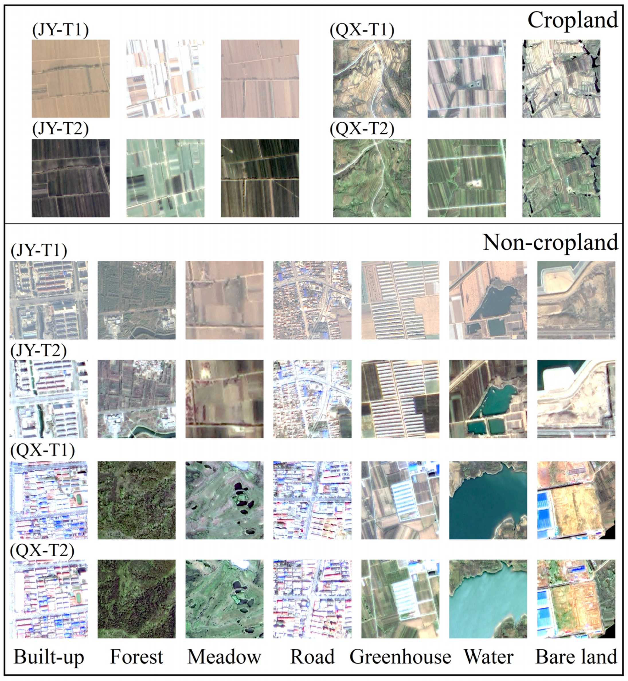
The cropland in the Juye region during the vigorous crop growth period has a spectral signature similar to forest and grassland, but its spatial contextual characteristics distinguish it from others. The cropland in Qixia during the non-vigorous crop growth period exhibits discernible spectral differences from forests with dense vegetation cover. The number of cropland parcels used as the ground truth in Juye and Qixia was 19,147 and 19,549, respectively. Figure 2 depicts the typical examples of cropland and non-cropland. In Juye, non-cropland areas include built-up, forest, water, road, meadow, greenhouse, and bare land, with built-up areas constituting the predominant non-cropland cover. The JY-T1 image set displays cropland at the initial sowing stage of winter wheat, characterized by bare soil. The JY-T2 image set depicts cropland during the robust growth phase of winter wheat. Similarly, in Qixia, non-cropland includes the same categories, with forests being the primary type of cover. The QX-T1 image set illustrates cropland at the beginning of summer maize sowing, appearing as bare soil. The cropland is shown in the vigorous growth stage of summer maize by the QX-T2 image set.
The cropland parcel data was converted into raster format, setting “cropland” pixels to 1, “non-cropland” pixels to 2, and pixels without remote sensing imagery coverage to 0. The GF-1 composite images and labeled results constituted the definitive cropland sample dataset. In addition, a grid-based method segmented each study area into sixteen sub-regions, which were randomly assigned to training, validation, and test sets (Figure 1). The training set was utilized to train the model, the validation set to optimize model parameters, and the test set to evaluate the model performance.

3. Methodology

3.1. Classifier Algorithms

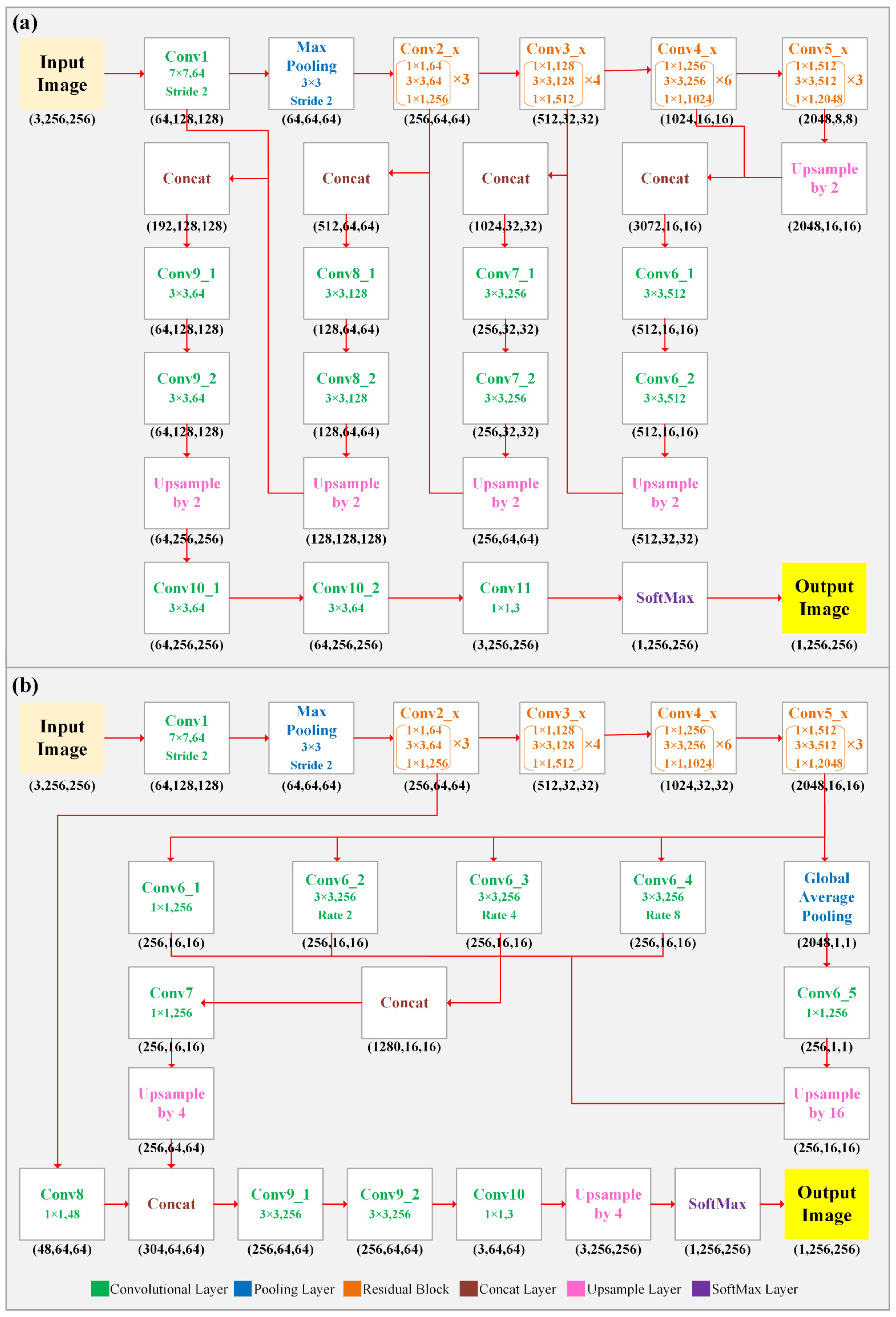
This study employed two DL classification algorithms and a traditional classification method to extract cropland areas from high-resolution satellite images. Specifically, two typical encoder–decoder semantic segmentation networks based on deep CNN architectures, namely UNet and DeepLabv3+, were selected due to their wide adoption for various applications involving RS classification [44,45,46]. The encoder components of UNet and DeepLabv3+ are excellent at extracting high-level features from input images. Meanwhile, the decoders are crucial in achieving fine-grained classification through the precise delineation of boundaries. ResNet-50 [47] was selected as the backbone architecture of the encoder for UNet and DeepLabv3+. Figure 3 shows the structures of the two DL models.
The UNet architecture utilizes ResNet-50 within its encoder for feature extraction, effectively capturing both deep and shallow feature maps of cropland. During the decoding stage, it progressively reconstructs the original dimensions of the input image through upsampling and convolution layers, simultaneously reducing the feature channels and enhancing detailed information for precise pixel-level predictions. Skip connections facilitate the integration of feature maps from the encoder with those of corresponding decoder layers, enabling efficient channel concatenation. This approach combines the edge information from shallow features with high-level spatial semantic information from deep features, ensuring to preserve more detail in the final segmentation output. Specifically, the high-resolution shallow features provide detailed edge information essential for accurately determining cropland boundaries, while the low-resolution deep features encompass long-range spatial dependencies that assist in recognizing croplands.
The encoding phase of DeepLabV3+ incorporates the ResNet-50 network for feature extraction and the Atrous Spatial Pyramid Pooling (ASPP) module. The ResNet-50 backbone facilitates feature learning and generates coarse feature maps, while the ASPP module produces high-level abstract feature maps through multi-scale convolutions. The ASPP module comprises a 1 × 1 convolution, three 3 × 3 convolutions at different dilation rates (2, 4, and 8), and a global average pooling layer. Atrous convolutions with varying dilation rates effectively capture contextual feature information from images, improving object recognition across different scales. In the decoding phase, the decoder meticulously reconstructs spatial details through two stages of 4× upsampling, sharpening object boundaries. The combination of shallow and deeply upsampled features enables accurate pixel-level prediction.
Additionally, the conventional OBIA-RF method was employed as a machine learning-based classifier for comparison with the DL algorithms. The object-based classification methods more effectively categorize objects based on multiple pixels with similar features, using the abundant feature information in high-resolution imagery. This approach proves more effective for extracting cropland from high-resolution images than traditional pixel-based classification techniques [48]. The RF employs an ensemble learning strategy that integrates multiple decision tree classifiers through bagging, significantly reducing the model’s prediction variance. It constructs each tree by selecting random samples and specific features, effectively minimizing the risk of overfitting [49]. In the OBIA-RF approach, the multi-resolution segmentation method is first applied to high-resolution images to isolate homogeneous objects. Subsequently, a diverse set of features is extracted from these segmented objects, including spectral features (mean and standard deviation), texture features (gray-level co-occurrence matrix), and geometric features (shape index, border index, and compactness). Finally, these features are fed into a parameterized RF for object-based classification.

3.2. Experiment Design

This study evaluates the performance of various classifiers for HHRS cropland extraction using datasets characterized by different band combinations, crop growth stages, and training data qualities. It aims to address the research questions posed at the end of Section 1 and achieve the research objectives. Section 3.1 provided a detailed overview of the three classifier types deployed in this study, which include two DL network architectures and one conventional classifier. In subsequent sections, Section 3.2.1 details the construction of samples with varying band combinations and temporal characteristics, Section 3.2.2 describes the creation of training samples of different qualities through sample quality control, and Section 3.2.3 outlines the model parameter settings and implementations for the three classifiers.

3.2.1. Sample Dataset Creation

To investigate the impact of various band combinations on HRRS cropland extraction, three different band combination sample datasets were created for each period of each study area using the GF-1 satellite images and the corresponding labeled samples. These datasets comprised the four-band combination of Near-Infrared–Red–Green–Blue (hereafter referred to as ALL), the three-band combination of Near-Infrared–Red–Green (referred to as NRG), and the three-band combination of Red–Green–Blue (referred to as RGB).
Additionally, to explore the impact of temporal characteristics on HRRS cropland extraction, two types of sample datasets were created for each study area, tailored to different growth stages of crops. The first type, T1 sample datasets (namely JY-T1 and QX-T1), represented the non-vigorous growth stage, whereas the second type, T2 sample datasets (comprising JY-T2 and QX-T2), depicted the vigorous growth stage. In each study area, models trained with T1 sample datasets were exclusively applied to classify test images from the non-vigorous growth stage for cropland extraction, while models trained with T2 sample datasets were solely utilized for classifying test images from the vigorous growth stage.

3.2.2. Sample Dataset Quality Control

This study created sample datasets with different label noise levels using the RGB band combination from the vigorous crop growth period of Juye and the non-vigorous crop growth period of Qixia. The grid tile was utilized as the basic unit to inject class label noise into the sample datasets within the training and validation areas. Through the statistical analysis of the cropland parcels’ acreages, the sizes of the mislabeled grid tiles in Juye and Qixia were determined as 80 × 80 pixels and 64 × 64 pixels, respectively. Seven noise levels (denoted from I to VII) were used, namely 2%, 5%, 10%, 20%, 30%, 40% and 50%. For each noise level, the number N of the mislabeled grid tiles was defined as follows:
N   =   S r n l s m g
where S represents the acreage of the training or validation areas, rnl denotes the noise level ratio and smg represents the acreage of each mislabeled grid tile. The resulting N tiles were randomly disseminated across the training and validation areas, and mislabeling was applied.
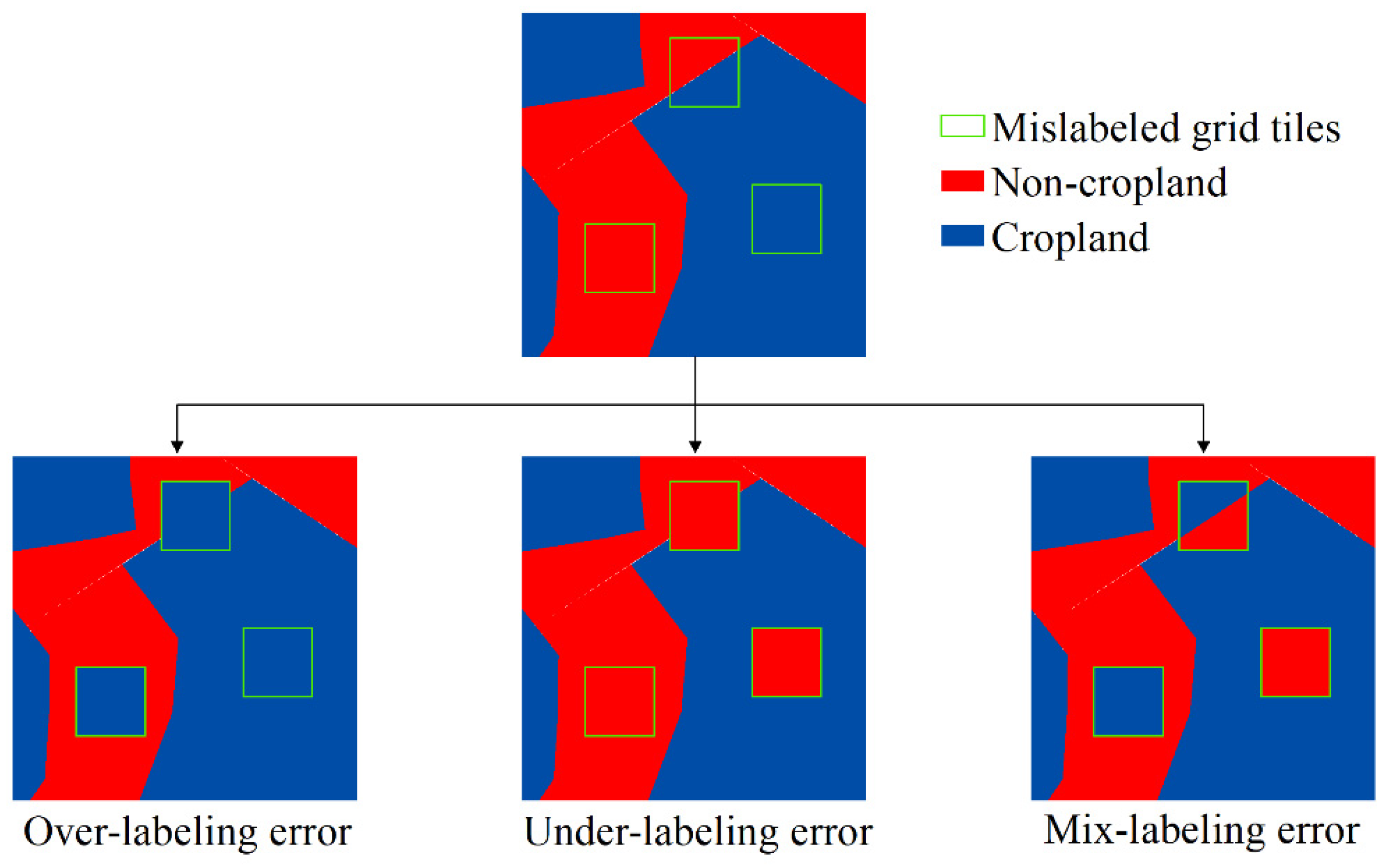
Furthermore, three error types, including over-labeling, under-labeling and mix-labeling errors (Figure 4), were defined. Over-labeling errors involved mislabeling non-cropland instances within the aforementioned mislabeled grid tiles as cropland. Under-labeling errors entailed cropland instances being mislabeled as non-cropland. Mix-labeling errors indicated a reversal of the label for each sample. One noticeable fact was that the degree of mislabeling varied for different error types, even under equal noise levels. To facilitate unbiased comparisons, the error area ratio was defined as follows:
r E A   =   s m s S
where S represents the acreage of the training or validation areas, and sms denotes the acreage of the mislabeled samples. The error area ratio was utilized as a metric to quantify the degree of mislabeling under various noise levels and error types.

3.2.3. Model Parameter Settings and Implementation

For the DL classification algorithms, the sample datasets in the training and validation areas were cropped into 256 × 256 pixel sample blocks with a 50% overlap and were used as inputs to the UNet and DeepLabv3+ models. Hence, 17,364 and 26,704 training sample blocks and 1780 and 2659 validation sample blocks were generated for Juye and Qixia, respectively. During training, the same hyper-parameters were utilized for all models. Specifically, the Adam optimizer [50] was used with an initial learning rate of 0.0001, a momentum of 0.9 and a batch size of 8. Each model was trained for a total of 20 epochs. A ResNet50 model pre-trained based on ImageNet was leveraged for initialization to accelerate the training process.
Regarding the OBIA-RF model’s implementation, the multi-resolution segmentation was parameterized using three key settings: scale, shape, and compactness, with respective values set to 50, 0.1, and 0.5. The RF classifier was configured with 500 trees, and the number of selected prediction variables was determined as the square root of the number of input features. The remaining parameters adhered to the default settings of the RF classifier.
The modeling process was implemented on the Python3.9 platform using the PyTorch1.1 library for UNet and DeepLabv3+, and the Scikit-learn library for RF. The computational work was conducted on the supercomputer at the National Supercomputing Center in Zhengzhou, featuring 3800 nodes. Each node boasts a 32-core X86 processor with a 2.0 GHz base frequency and four DCU accelerators with a GPU-like architecture, each comprising 60 Compute Units. Among these nodes, 2600 have 128 GB of memory, 1200 have 256 GB, and all are equipped with 16 GB of graphics memory. Four DCU accelerators were utilized during the deep learning model’s training phase, while a single DCU accelerator was utilized for prediction.

3.3. Model Evaluation

To evaluate and compare the different models’ performance on HRRS cropland extraction, five common quantitative metrics were employed: overall accuracy (OA), kappa, producer’s accuracy (PA), user’s accuracy (UA), and F1-score. In addition, each model underwent five iterative runs to ensure stable accuracy estimations, from which the average performance metrics were calculated.

4. Results

4.1. Effect of Classifier Selection on High-Resolution Cropland Extraction

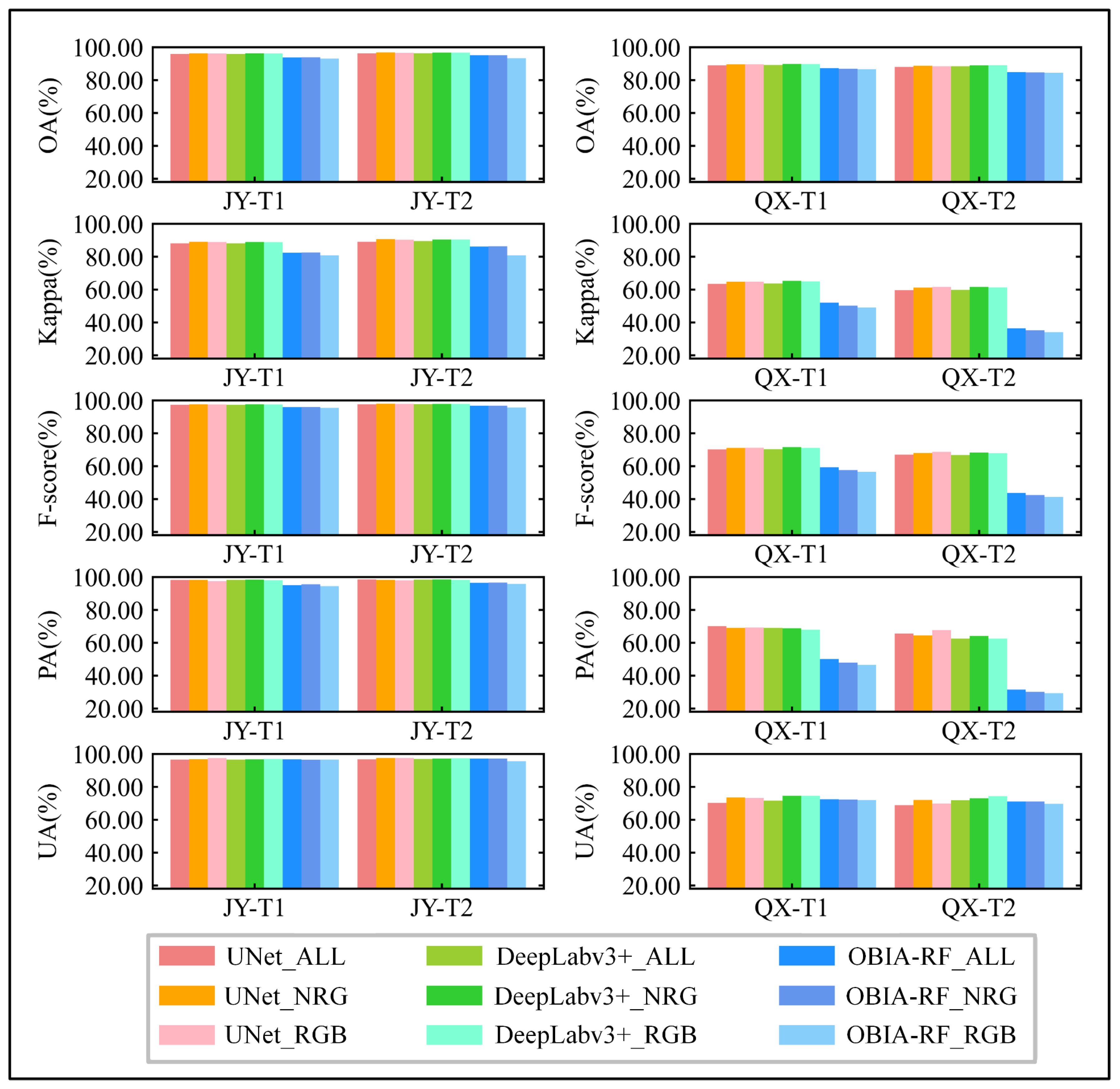
Figure 5 and Table 3 illustrate the quantitative accuracy assessment results for HRRS cropland extraction. For the test set of each study area, a total of 18 cropland extraction outcomes were obtained based on various classifier algorithms, band combinations, and crop growth stages. Specifically, three classifier algorithms were compared: two DL models, UNet and DeepLabv3+, alongside a conventional classification algorithm, OBIA-RF. The band combinations included three types: ALL (Near-Infrared–Red–Green–Blue), NRG (Near-Infrared–Red–Green), and RGB (Red–Green–Blue). The crop growth stages were divided into two phases: the non-vigorous crop growth period (T1) and the vigorous crop growth period (T2). Overall, across both simple agricultural landscapes with flat terrain and complex mountainous regions, and regardless of crop growth stages, the cropland extraction results from the UNet and DeepLabv3+ models exhibited minimal differences, outperforming the OBIA-RF model. However, the extent of improvement achieved by the DL models varied across the different study areas and crop growth periods.
In the plain area Juye, characterized by uncomplicated agricultural landscapes, flat topography, and regular cropland parcels, cropland is easily distinguishable from other land cover types. The traditional OBIA-RF classification model achieved excellent classification performance for both non-vigorous (T1) and vigorous (T2) crop growth periods. The UNet and DeepLabv3+ methods exhibited slight improvements over the OBIA-RF algorithm. Specifically, the OBIA-RF model achieved an overall accuracy of over 93.00%, a Kappa coefficient above 0.80, and an F1-score exceeding 95.00%, indicating high classification accuracy. In contrast, the UNet and DeepLabv3+ models achieved an overall accuracy of over 95.00%, a Kappa coefficient above 0.88, and an F1-score surpassing 97.00%, indicating a slight performance boost over the OBIA-RF algorithm.
In the mountainous area Qixia, with its fragmented terrain and complex agricultural landscapes, the OBIA-RF model’s cropland extraction performance was substantially lower than the two DL models. This indicates that the shallow classifiers based on manually crafted features struggled to effectively recognize cropland in HRRS imagery from such challenging terrains. Notably, both UNet and DeepLabv3+ models significantly outperformed the OBIA-RF model, with negligible differences observed between them. In particular, the two DL models demonstrated substantial improvements over the OBIA-RF algorithm in terms of cropland’s PA. Specifically, in the non-vigorous crop growth periods, the maximum improvements in PA achieved by the UNet and DeepLabv3+ models were 22.71% and 21.46%, respectively. These improvements were even more pronounced in the vigorous crop growth period, reaching 38.31% for the UNet and 33.95% for the DeepLabv3+. Accordingly, DL models more effectively leveraged the rich details in HRRS imagery than the OBIA-RF algorithm, achieving superior accuracy in cropland extraction.

4.2. Effect of Band Combination on High-Resolution Cropland Extraction

In the plain area Juye, the cropland extraction accuracies of the two DL models, UNet and DeepLabv3+, exhibited no significant difference across different band combinations. This indicated that both DL algorithms could extract deep abstract features and contextual semantic information from the HRRS imagery, which were insensitive to different band combinations. The OBIA-RF model showed comparable cropland extraction performance between the ALL and NRG band combinations. However, the accuracies of the RGB band combination were lower than those of the other two band combinations, indicating that the NIR spectral information played a crucial role in high-resolution cropland extraction using the OBIA-RF model in Juye. Specifically, in both the non-vigorous and vigorous crop growth periods, the differences in OA, Kappa coefficient, and F1-score across the three different band combinations were minimal for both UNet and DeepLabv3+ models. For the non-vigorous crop growth period, the maximum differences in OA, Kappa, and F1-score across the three different band combinations were merely 0.29%, 0.88%, and 0.18% for UNet, and 0.28%, 0.82%, and 0.18% for DeepLabv3+, respectively. The maximum differences for the vigorous crop growth period were 0.53%, 1.68%, and 0.32% for UNet, and 0.30%, 0.87%, and 0.19% for DeepLabv3+. For the OBIA-RF model, the highest and lowest classification accuracies were obtained using the NRG and RGB band combinations, respectively. The differences between these two combinations in OA, Kappa, and F1-score were 0.73%, 1.76%, and 0.50% for the non-vigorous crop growth period, and were 1.86%, 5.44%, and 1.19% for the vigorous crop growth period, respectively.
In the mountainous area Qixia, the OBIA-RF model consistently achieved the highest cropland extraction accuracies using the ALL band combination, regardless of whether it was during the non-vigorous or vigorous crop growth periods. The NRG band combination performed merely well, while the RGB band combination yielded the lowest accuracies. This suggested that both NIR and B band spectral information contributed to the improvement of cropland extraction using the OBIA-RF model in Qixia, with the NIR band having a more pronounced impact than the B band. Specifically, in the non-vigorous crop growth period, the maximum differences in OA, Kappa, and F1-score across different band combinations were 0.51%, 2.90%, and 2.76%, respectively. In the vigorous crop growth period, these differences were 0.40%, 2.40%, and 2.38%. For the DL models, the differences in cropland extraction between RGB and NRG band combinations were insignificant, but both showed marginal improvements over the ALL band combination. For both the non-vigorous and vigorous crop growth periods, the maximum differences in OA, Kappa, and F1-score for both UNet and DeepLabv3+ models across different band combinations did not exceed 0.72%, 1.93%, and 1.64%, respectively. Accordingly, both in the plain and mountainous regions, the two DL models employed in this study exhibited less sensitivity to different band combinations than the OBIA-RF model.

4.3. Effect of Temporal Characteristics on High-Resolution Cropland Extraction

The HRRS cropland extraction results varied across different crop growth stages. In the plain area Juye, the cropland extraction accuracies in the vigorous crop growth period were marginally higher than those in the non-vigorous period. However, in the mountainous area Qixia, the accuracies in the non-vigorous crop growth period were significantly superior to those in the vigorous period. In the plain area, cropland in the non-vigorous period was more prone to being omitted than in the vigorous period. In the mountainous region, where cropland and forest dominated the landscape, it was relatively straightforward to distinguish between the two in the non-vigorous crop growth period, as the forest was in a vigorous growth stage at the time. However, during the vigorous crop growth period, both cropland and forest were covered in dense vegetation. Thus, cropland was often misclassified as forest, leading to lower classification accuracy compared to the non-vigorous crop growth period. Notably, the UNet and DeepLabv3+ models demonstrated substantial performance improvements over the OBIA-RF model during the vigorous crop growth period in complex mountainous terrain, highlighting their superior feature learning capabilities in areas with high landscape heterogeneity and low spectral separability.
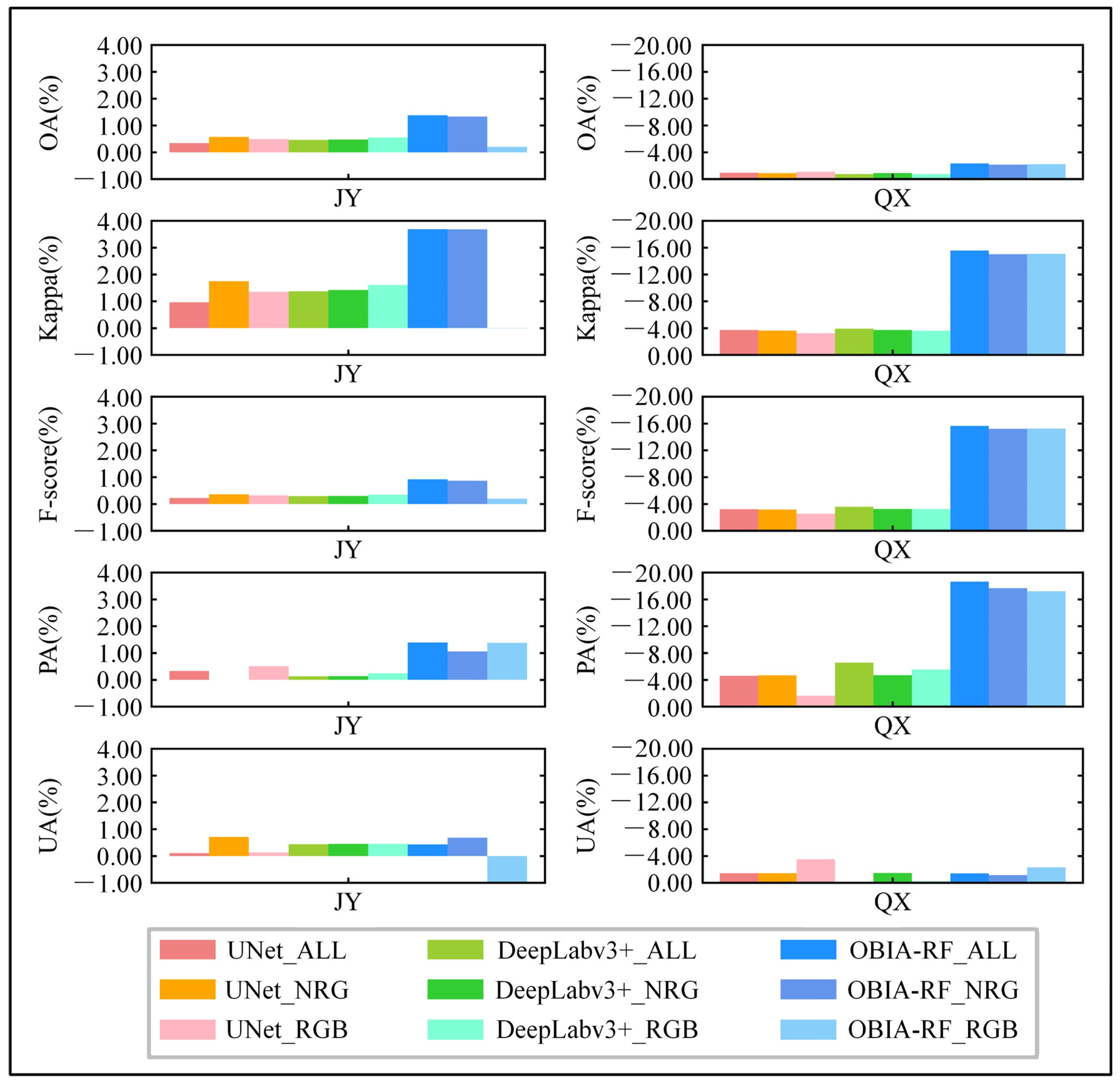
To further analyze the different classifiers’ responses to temporal characteristics, the accuracy differences between the two periods were calculated by subtracting the accuracies during the non-vigorous crop growth period from those during the vigorous crop growth period (Figure 6). The results showed that the accuracy differences between the two periods for OBIA-RF were greater than those for the UNet and DeepLabv3+ models in both study areas. This indicated that the OBIA-RF model was more sensitive to temporal changes than the DL models. This could be attributed to OBIA-RF’s reliance on manually designed input features, such as spectral, texture, and geometric features, for classification, which are highly susceptible to variations across different crop growth stages. In contrast, UNet and DeepLabv3+ automatically learn spatial context and multi-scale features via deep convolutional structures, enabling more stable feature representation and enhanced robustness to temporal variations.
Additionally, the accuracy differences between the two periods in the plain area were smaller than in the mountainous region. In the plain region, for the OBIA-RF model, the maximum increase in OA from the non-vigorous to vigorous periods was only 1.38%, with Kappa increasing by a maximum of 3.69%, and F1-score increasing by a maximum of 0.92%. For the UNet model, these increases were 0.57% in OA, 1.75% in Kappa, and 0.36% in F1-score. For the DeepLabv3+ model, the increases were 0.55% in OA, 1.61% in Kappa, and 0.35% in F1-score. In the mountainous region, the improvement in cropland extraction performance from the vigorous to the non-vigorous period was more pronounced, especially in cropland’s PA. Under the OBIA-RF model, cropland’s PA increased by up to 18.63%, while the maximum increases under the UNet and DeepLabv3+ models were 4.66% and 6.56%, respectively. These findings indicated that, compared to OBIA-RF, deep learning models could leverage spatial contextual information to mitigate the effects of temporal variation, thereby achieving more stable performance.

4.4. Effect of Class Mislabeling on High-Resolution Cropland Extraction

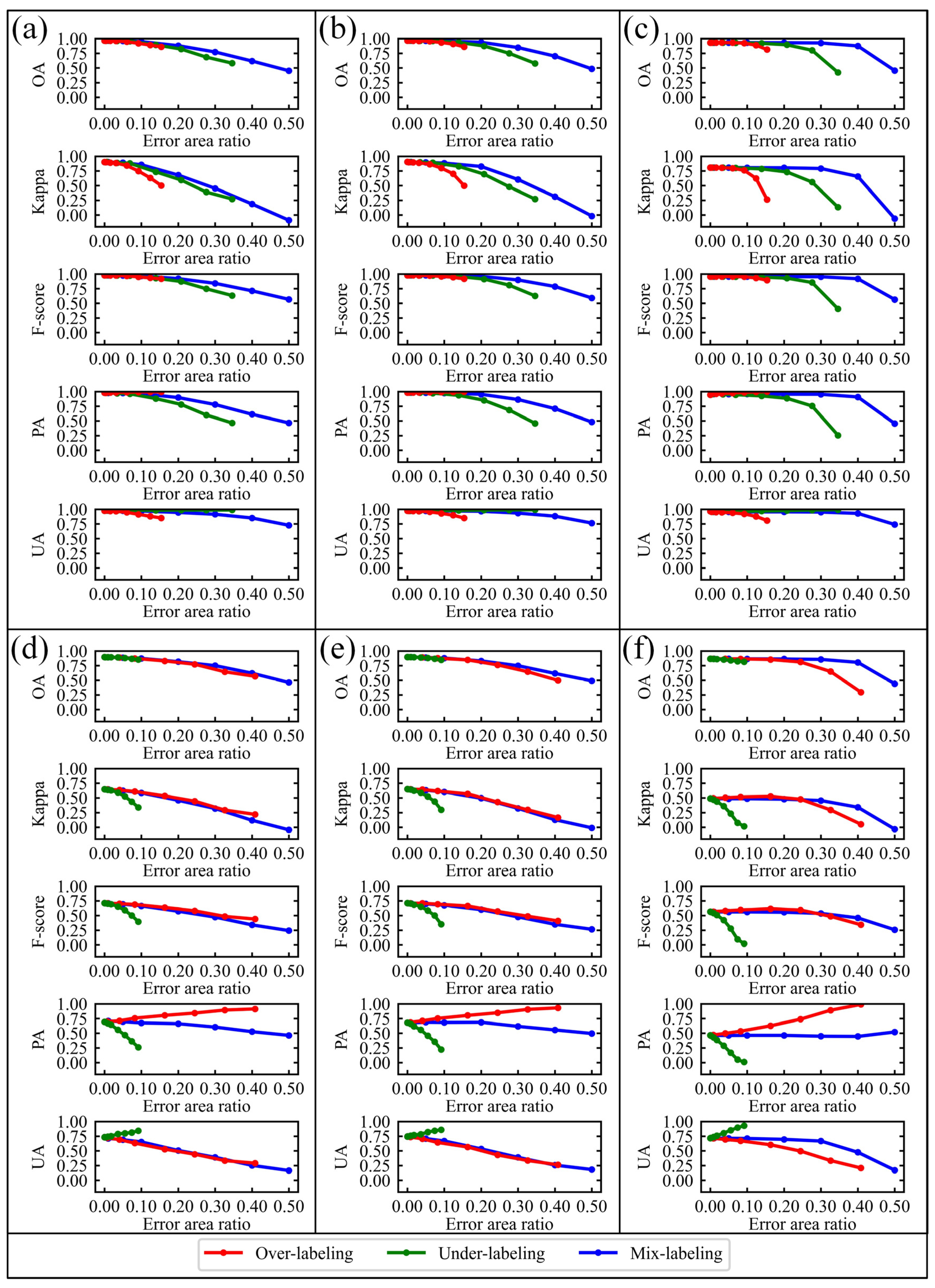
Table 4 illustrates the error area ratios under different noise levels and different error types for the two study areas. Figure 7 provides a quantitative depiction of the impact of mislabeled samples on HRRS cropland extraction. It was evident that as the proportion of mislabeled samples increased, the classification accuracies of the three classifier algorithms (Deeplabv3+, UNet, and OBIA-RF) declined. The trends in accuracy reduction for Deeplabv3+ and UNet were relatively similar, whereas the OBIA-RF model exhibited a markedly distinct trend. At lower error rates, the impact of mislabeled samples on cropland extraction accuracies of the three classifier algorithms was negligible. However, with increasing error rates, the rates of decline for OA, Kappa, and F1-score became increasingly pronounced, with OBIA-RF exhibiting a steeper drop than Deeplabv3+ and UNet. As a traditional machine learning classifier, OBIA-RF is relatively sensitive to sample label noise. This is because OBIA-RF integrates a large number of decision trees, and incorrect labels can mislead these trees, resulting in the model overfitting to noisy samples and ultimately causing a significant decline in overall performance. In contrast, the UNet and Deeplabv3+ models possess stronger feature representation and spatial contextual modeling capabilities, which can alleviate the adverse effects of noisy labels to some extent and exhibit greater robustness.
The effect of class mislabeling on high-resolution cropland extraction varied among the three types of mislabeling errors in each study area. For the plain area Juye, over-labeling errors had the highest impact on OA, Kappa, and F1-score among the three mislabeling types, followed by under-labeling and mix-labeling errors. A short plateau could be observed at low noise levels for each mislabeling type under the three classifier algorithms (less than 2% loss in OA from error-free sample data to 5% mislabeled), indicating that small amounts of class mislabeling had a minor effect on cropland extraction accuracy. Interestingly, the presence of mislabeled instances occasionally led to an increase in accuracy. For instance, under the UNet, Deeplabv3+, and OBIA-RF models, a 15.4% over-labeling error resulted in increases of 1.47%, 1.29%, and 5.47% in cropland’s PA, respectively. However, this led to more substantial decline in cropland’s UA, which decreased by 12.52%, 12.39%, and 15.80%. This could be attributed to the fact that the over-labeled sample dataset would cause slightly fewer omissions of cropland pixels and many more misclassifications of non-cropland pixels compared to the error-free sample dataset. On the contrary, under-labeling caused a minor improvement in cropland’s UA, along with a substantial reduction in cropland’s PA yet. Consequently, both over-labeling and under-labeling had a passive impact on overall classification performance. Moreover, compared to under-labeling, over-labeling reduced the number of minority class (non-cropland) sample pixels and resulted in greater loss in OA, Kappa, and F1-score, indicating that all three classifier algorithms were more tolerant of under-labeling of the majority class (cropland) better than that of the minority class (non-cropland). The mix-labeling error had adverse effects on both cropland’s PA and UA, but to a lesser extent than pure over-labeling or under-labeling. Hence, it had the least overall impact among the three error types.
Similar observations were made in the mountainous area Qixia, where the overall classification accuracy under all error types declined with the increase in the proportion of mislabeled samples. The emergence of flat zones at error area ratios below 5% signified the minor effect of class label noise on overall classification accuracy at low levels. Generally, mix-labeling caused the smallest effect on the overall accuracy among the three error types, followed by over-labeling and under-labeling, further verifying that under-labeling of the minority class (cropland) resulted in greater losses in overall classification accuracy compared to under-labeling of the majority class (non-cropland). From the perspective of cropland’s classification accuracy, over-labeling errors resulted in a more significant decrease in cropland’s UA than the increase in cropland’s PA. Accordingly, the under-labeled sample dataset slightly increased cropland’s UA but contributed to a steeper reduction in cropland’s PA. Additionally, mix-labeling degraded both the cropland’s PA and UA, with the losses in UA being considerably greater than those in PA. For example, under the UNet, Deeplabv3+, and OBIA-RF models, a 40% mix-labeling error resulted in losses of 48.08%, 48.92%, and 24.31% in cropland’s UA and decreases of 16.55%, 12.37%, and 1.97% in PA, respectively. These could be because mix-labeled pixels in the sample dataset comprised a majority of over-labeled pixels (80%) and a minority of under-labeled pixels (20%) (Table 4).
In summary, both OBIA-RF and the two deep learning models exhibited strong robustness under low label noise. However, when exposed to high levels of label noise, OBIA-RF became more susceptible to performance degradation, with its accuracy declining more markedly. This is primarily due to OBIA-RF’s reliance on sample distribution and decision tree output, making it more prone to misclassification when labels are incorrect. In contrast, deep learning models benefit from advanced feature extraction and spatial relationship modeling capabilities, which provide greater tolerance to label noise and result in a relatively slower decline in accuracy. Overall, for cropland extraction from high-resolution remote sensing images, deep learning algorithms demonstrated superior robustness and stability in the presence of noisy labels.

5. Discussion

5.1. Analysis on Patch Size of Sample Blocks for Deep Learning Methods

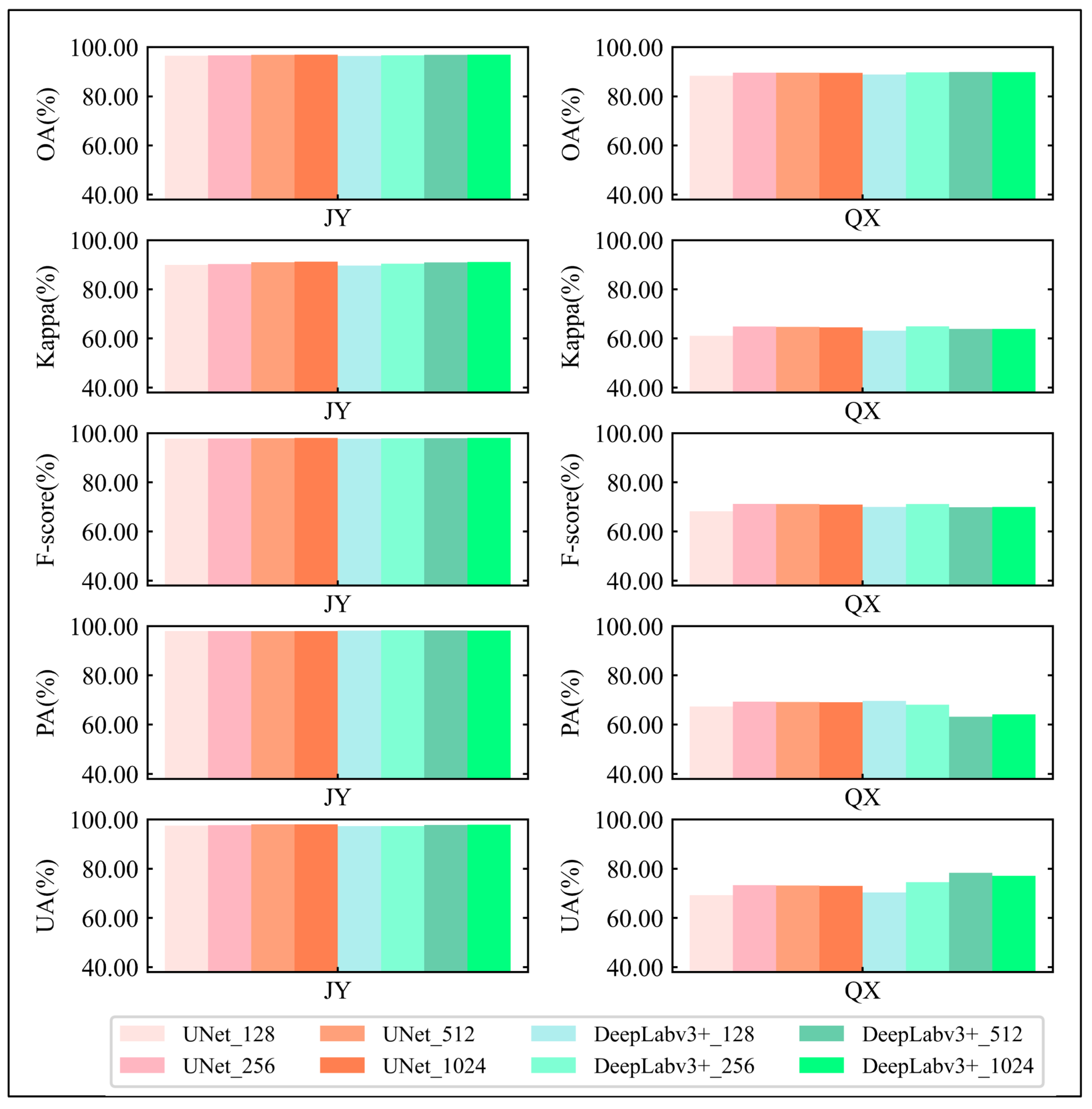
The relationship between the patch size of sample blocks and the performance of the DL methods was assessed. Sample blocks with patch sizes 128 × 128, 256 × 256, 512 × 512, and 1024 × 1024 were created using the RGB sample datasets in the vigorous crop growth period of Juye and the non-vigorous crop growth period of Qixia. Figure 8 illustrates the cropland extraction accuracy results under datasets with sample blocks of different patch sizes. It can be observed that in the plain area Juye, which is characterized by regular cropland parcels, both UNet and DeepLabv3+ achieved high accuracies with no significant difference across the four patch sizes. This indicates that the choice of patch size for the sample block did not affect the performance of DL models in extracting cropland in plain areas with regular cropland patterns and simple agricultural landscapes.
In the mountainous area Qixia, characterized by fragmented cropland distributions and complex agricultural landscapes, the two DL models performed differently. Under the UNet model, the accuracy at the 128 × 128 patch size was lower compared to the other three larger scales. However, there were no significant differences in accuracy among 256 × 256, 512 × 512, and 1024 × 1024 patch sizes. This suggested that a too-small patch size was not conducive to learning cropland features for the UNet model, but once the patch size reached a certain threshold (256 × 256), its variation had minimal impact on cropland extraction performance. For the Deeplabv3+ model, cropland’s PA decreased as the patch size increased, while UA increased, implying that larger patch sizes under the DeepLabv3+ model led to more cropland omissions but fewer cropland misclassifications. However, for different patch sizes, there were slight fluctuations in the values of overall metrics such as OA, kappa, and F1-score.

5.2. Analysis on Data Augmentation for Deep Learning Methods

Data augmentation is a common strategy in DL applications to increase the amount and the diversity of the training data to enhance the classification accuracies [51,52]. This study further investigated the impact of data augmentation on the high-resolution cropland extraction based on the DL methods in different agricultural landscapes. Augmented sample datasets were generated using spatial augmentation techniques such as flipping and rotation based on the RGB band combination in the vigorous crop growth period of Juye and the non-vigorous crop growth period of Qixia, respectively. Table 5 showed that data augmentation slightly improved HRRS cropland extraction accuracies in the plain area Juye for both UNet and DeepLabv3+ models, whereas it marginally reduced accuracies in the mountainous area Qixia. This could be attributed to the fact that spatial augmentation methods like flipping and rotation enriched the training samples in simpler agricultural landscapes, thereby facilitating cropland extraction. However, in the mountainous areas with complex cropland landscapes, these methods increase the complexity of the sample datasets, potentially hindering the DL models’ ability to learn cropland features, leading to reduced cropland extraction accuracy. Therefore, data augmentation strategies are not always effective in enhancing classification accuracy, and should be carefully considered in practical operational applications.

5.3. Analysis of Classifier Robustness

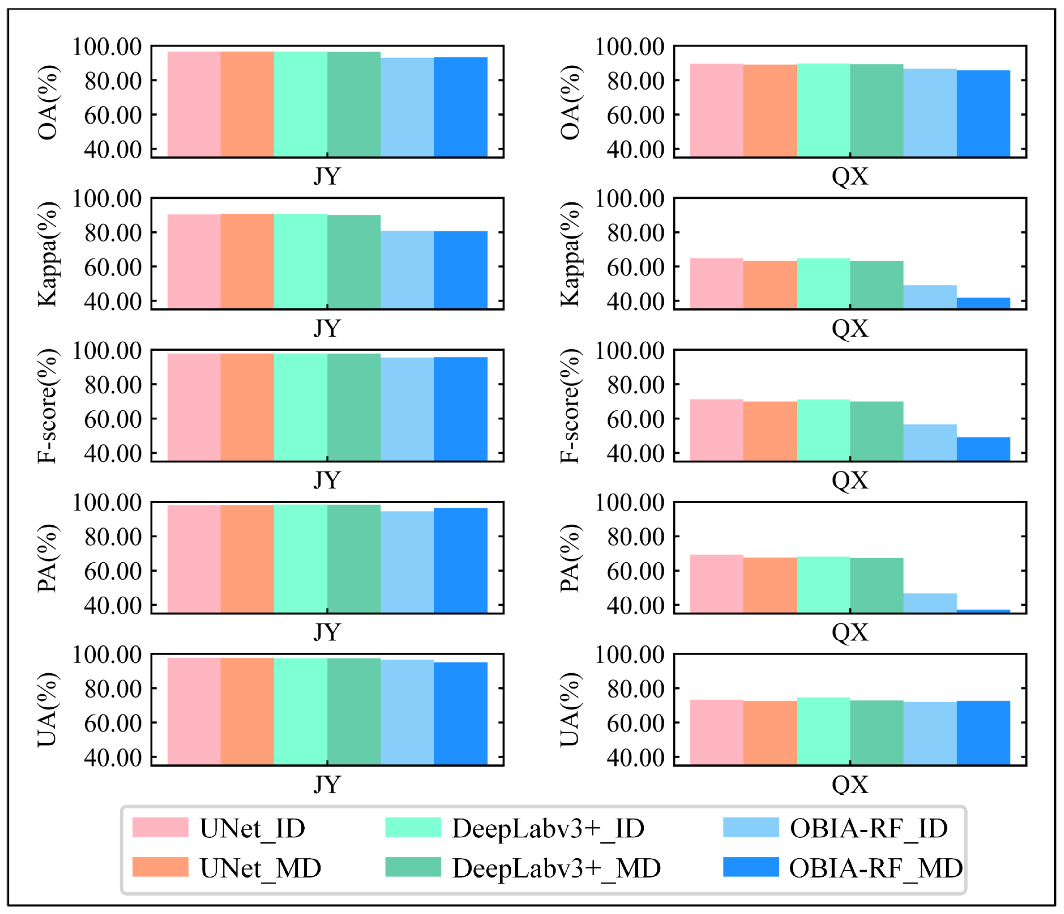
To assess the robustness of the three classifiers—UNet, Deeplabv3+, and OBIA-RF, this study combined the RGB training samples from the plain area Juye and the mountainous area Qixia from the vigorous and non-vigorous crop growth periods to create a mixed sample training dataset based on the mixed agricultural landscapes and crop growth stages. The models trained on the mixed sample training dataset were subsequently evaluated on GF-1 images from Juye’s vigorous and Qixia’s non-vigorous crop growth periods, respectively. The classification performance on the mixed dataset was analyzed for each classifier and compared to the results of the individual training sample dataset from the individual agricultural landscape and crop growth stage (as displayed in Figure 9). For the plain area Juye, the UNet and DeepLabv3+ models produced similar results between the mixed and individual datasets. However, the OBIA-RF model demonstrated higher PA and lower UA on the mixed dataset compared to the individual dataset, while overall metrics like OA, Kappa, and F1-score were comparable on both datasets. In the mountainous region Qixia, the UNet and DeepLabv3+ showed marginally lower cropland extraction accuracies on the mixed dataset than on the individual dataset, while the OBIA-RF model exhibited a notable decrease in accuracy. Overall, compared to the individual dataset, the mixed dataset presented greater challenges in learning complex cropland features in the mountainous area, resulting in a decrease in the HRRS cropland extraction accuracy for all three models. However, UNet and DeepLabv3+ demonstrated better learning of stable cropland features than OBIA-RF, with smaller decreases in accuracy, indicating stronger model robustness.
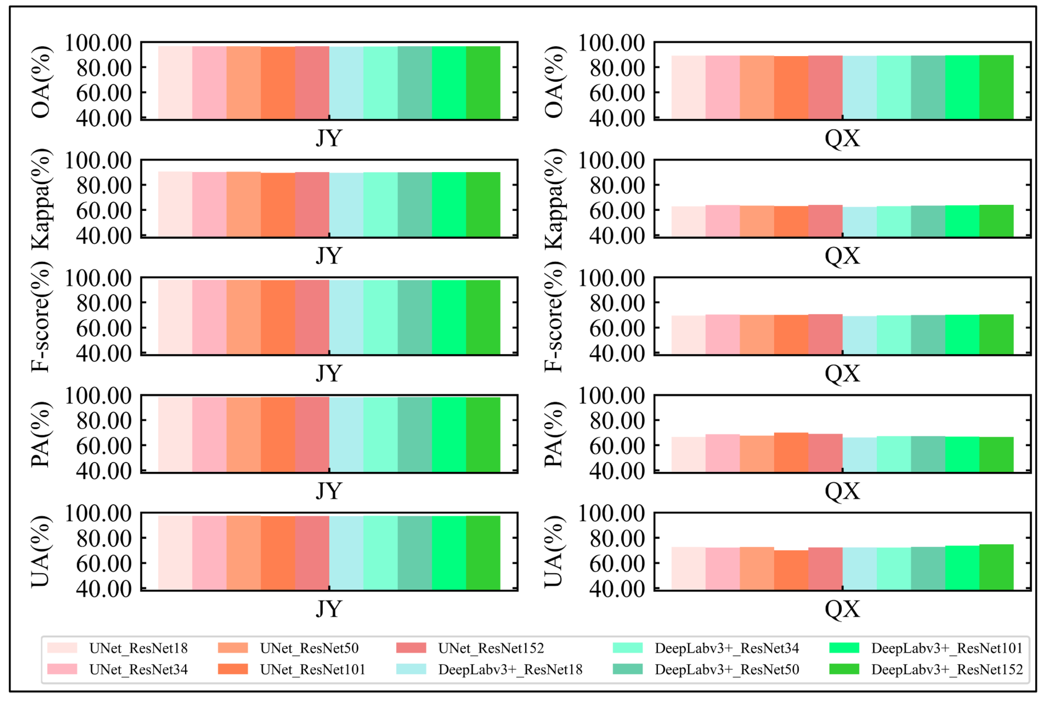
Furthermore, this study evaluated how different depths of the ResNet backbone architecture affected high-resolution cropland extraction results within UNet and DeepLabv3+ models (as displayed in Figure 10). The mixed dataset was used for training, and GF-1 images from Juye’s vigorous crop growth period and Qixia’s non-vigorous crop growth period served as the test dataset. ResNet18, ResNet34, ResNet50, ResNet101, and ResNet152 were utilized as the backbone architectures, respectively. The findings indicated that the depth of the ResNet backbone architecture did not substantially impact cropland extraction accuracy, implying that these two DL models are not sensitive to the ResNet depth variations for the high-resolution cropland extraction.

5.4. Applicability of Different Classifiers

In both the plain area Juye and the mountainous area Qixia, the UNet and DeepLabv3+ DL models outperformed the OBIA-RF algorithm in cropland classification. In Juye, characterized by relatively simple agricultural landscapes and regular cropland parcels, the OBIA-RF algorithm exhibited excellent performance across various time periods, with overall accuracy ranging from 93.08% to 95.14%. The enhancement in overall accuracy of the DL models over the OBIA-RF model was modest, ranging from 1.16% to 3.38%. In Qixia, with its complex agricultural landscapes and fragmented cropland parcels, the OBIA-RF algorithm performed poorly, particularly with a severe underestimation of cropland. Deep learning models can significantly rectify this issue, improving cropland’s PA by 18.95% to 38.31%.
The computational efficiency of the three classifiers was further evaluated and compared based on the RGB sample datasets in the vigorous crop growth period of Juye and the non-vigorous crop growth period of Qixia. Table 6 showed that the training times of UNet and DeepLabv3+ were comparable, with an average time of 4.57 and 4.71 h for Juye and 7.76 and 8.00 h for Qixia. The training time required for the OBIA-RF method was approximately one-tenth of that required for the DL approaches. With regard to the inference time on the test set, the two DL methods did not significantly differ, taking roughly 2 to 3 times longer than the OBIA-RF method.
Considering both classification accuracy and computational efficiency, the traditional OBIA-RF algorithm emerges as an appropriate selection for plain areas with regular cropland patterns, mainly when mapping accuracy demands are not extremely high and there is limited hardware capability for training DL models. In contrast, in croplands characterized by complex agricultural landscapes, the UNet and DeepLabv3+ models are preferable due to their ability to achieve higher classification accuracy.
Further comparison between these two deep learning models revealed that DeepLabv3+ achieved slightly higher accuracies than UNet across most evaluation scenarios. Nevertheless, the differences were negligible, with the overall accuracy difference of no more than 0.50% and the kappa coefficient difference of no more than 0.60%. Due to the incorporation of a more complex ASPP module, DeepLabv3+ possesses a larger number of parameters compared to UNet, resulting in longer training and inference time. From the architectural perspective, both UNet and DeepLabv3+ are encoder–decoder-based semantic segmentation models. UNet employs a symmetric encoder–decoder structure with skip connections to preserve high-resolution spatial details from the early layers and combine them with the deeper, semantically rich features. This design facilitates fine-grained classification, making it particularly suitable for high-resolution cropland extraction. In contrast, DeepLabv3+ enhances cropland feature representation by incorporating the ASPP module within its encoder, which explicitly captures multi-scale contextual information through convolutions with different dilation rates. This enables effective recognition of cropland objects at multiple scales but increases model complexity and computational demand. Despite their architectural differences, both models are capable of learning sufficient spatial and semantic features from the training data for the specific task of cropland extraction from high-resolution imagery. Consequently, their performance in terms of accuracy is nearly identical across diverse agricultural landscapes. The slight accuracy advantage of DeepLabv3+ could be attributed to its explicit multi-scale modeling, whereas the superior computational efficiency of UNet makes it a more practical choice for scenarios requiring faster inference, especially given the negligible difference in accuracy.

5.5. Contributions and Limitations of the Current Study

This study investigated the effects of classifiers and sample data characteristics, including band combinations, temporal characteristics, and class mislabeling, on high-resolution cropland extraction across different agricultural landscapes, such as plain and mountainous regions. The findings offer valuable insights for researchers designing experiments on high-resolution cropland extraction. Additionally, for agricultural practitioners, understanding how various classifiers, band combinations, temporal characteristics, and training sample qualities impact the performance of cropland extraction is crucial for efficiently, timely, and accurately identifying cropland spatial distributions. This enables more informed decision-making and resource management. For policymakers, reliable cropland monitoring data serves as a robust scientific foundation for policy development, assisting the government in developing more effective agricultural policies and response strategies that support food security and sustainable development goals.
However, this study focused on two representative study areas in northern China, known for winter wheat and summer maize cultivation. The applicability of the findings to the southern regions, predominantly rice-growing, and to significantly different agricultural landscapes requires further exploration. Moreover, this study has not evaluated the performance of different algorithms across large-scale land-use areas. Future research should assess these algorithms using a wider range of land-use types and larger spatial extents to more effectively determine the model’s generalizability and practical applicability. Furthermore, the determinants of high-resolution cropland classification are not only limited to external factors such as classifier algorithms, spectral information, temporal characteristics and training data quality, but also include intrinsic characteristics such as crop growing environment, cropland parcel size and surface heterogeneity. Future research should explore how these intrinsic factors affect the performance of DL models in HRRS cropland extraction.

6. Conclusions

This study provided valuable insights into the impact of classifier selection, band combination, temporal characteristics and class mislabeling on HRRS cropland extraction to facilitate the design of practical operational implementations. The main conclusions are as follows:
(1)
The UNet and DeepLabv3+ models demonstrated superior performance to OBIA-RF for HRRS cropland extraction across various crop growth stages in both simple and complex agricultural landscapes, highlighting the advantages of DL algorithms in such applications. Furthermore, the performance evaluation conducted on a mixed sample dataset (containing samples from different agricultural landscapes and crop growth stages) showed that the DL models were more robust than OBIA-RF.
(2)
Different band combinations had negligible effects on the cropland extraction performance of the UNet and DeepLabv3+ models, indicating that these models could effectively learn deep abstract features and contextual semantic information and were insensitive to band combination changes. Conversely, OBIA-RF showed varying levels of accuracy across different band combinations. Specifically, Near-Infrared–Red–Green–Blue and Near-Infrared–Red–Green outperformed Red–Green–Blue, reflecting the significance of the NIR band’s information in cropland extraction when the OBIA-RF model was used.
(3)
From the perspective of temporal characteristics, the cropland mapping results were different when the corresponding RS images were from different crop growth stages, with smaller discrepancies in plain areas compared to mountainous regions between the vigorous and non-vigorous crop growth periods. Moreover, OBIA-RF was more sensitive to the temporal changes than UNet and DeepLabv3+.
(4)
In terms of class mislabeling on the high-resolution cropland extraction, the classification performance of all three models (UNet, DeepLabv3+ and OBIA-RF) remained relatively resilient to training data noise with up to 5% mislabeling. Beyond this threshold, the classification accuracy declined as the error rate increased. While UNet and DeepLabv3+ exhibited similar trends of performance degradation, OBIA-RF experienced a more significant drop in accuracy.
(5)
Data augmentation strategies for HRRS cropland extraction do not significantly improve the classification accuracy of UNet and DeepLabv3+. In complex mountainous areas, these strategies even reduced performance. Thus, it is advised that these strategies can be judiciously applied in practical applications. Furthermore, UNet and DeepLabv3+ had relatively low sensitivity to the patch size of sample blocks and the depth of the ResNet backbone.

Author Contributions

Conceptualization, D.Z., X.Z. and Y.P.; methodology, D.Z., Y.P. and Q.L.; formal analysis, D.Z., X.Z., H.G. and H.W.; investigation, Q.L.; writing—original draft preparation, D.Z.; writing—review and editing, D.Z., X.Z., Y.P., H.G. and H.W.; visualization, D.Z.; supervision, D.Z. and X.Z.; funding acquisition, D.Z. and H.G. All authors have read and agreed to the published version of the manuscript.

Funding

This research was funded by the National Natural Science Foundation of China (No. 42501427), the Key Research and Development Special Projects in Henan Province (No. 241111212300, No. 221111320600), the Key R&D and Promotion Special Projects of Henan Province (No. 242102321024), and the Postgraduate Education Reform and Quality Improvement Project of Henan Province (No. YJS2025GZZ06).

Data Availability Statement

Data will be made available on request.

Conflicts of Interest

The authors declare no conflicts of interest.

References

  1. Patil, P.; Gumma, M.K. A review of the available land cover and cropland maps for South Asia. Agriculture 2018, 8, 111. [Google Scholar] [CrossRef]
  2. Zhao, J.; Chen, P.J.C. High-resolution cropland mapping in China’s Huang-Huai-Hai Plain: The coupling of machine learning methods and prior information. Comput. Electron. Agric. 2024, 224, 109225. [Google Scholar] [CrossRef]
  3. Karthikeyan, L.; Chawla, I.; Mishra, A.K. A review of remote sensing applications in agriculture for food security: Crop growth and yield, irrigation, and crop losses. J. Hydrol. 2020, 586, 124905. [Google Scholar] [CrossRef]
  4. LeCun, Y.; Bengio, Y.; Hinton, G. Deep learning. Nature 2015, 521, 436–444. [Google Scholar] [CrossRef] [PubMed]
  5. Zhang, X.; Zhou, Y.n.; Luo, J. Deep learning for processing and analysis of remote sensing big data: A technical review. Big Earth Data 2022, 6, 527–560. [Google Scholar] [CrossRef]
  6. Hosseiny, B.; Mahdianpari, M.; Hemati, M.; Radman, A.; Mohammadimanesh, F.; Chanussot, J. Beyond supervised learning in remote sensing: A systematic review of deep learning approaches. IEEE J. Sel. Top. Appl. Earth Obs. Remote Sens. 2023, 17, 1035–1052. [Google Scholar] [CrossRef]
  7. Zhang, L.; Zhang, L.; Du, B. Deep learning for remote sensing data: A technical tutorial on the state of the art. IEEE Geosci. Remote Sens. Mag. 2016, 4, 22–40. [Google Scholar] [CrossRef]
  8. Cao, F.; Xing, B.; Luo, J.; Li, D.; Qian, Y.; Zhang, C.; Bai, H.; Zhang, H. An Efficient Object Detection Algorithm Based on Improved YOLOv5 for High-Spatial-Resolution Remote Sensing Images. Remote Sens. 2023, 15, 3755. [Google Scholar] [CrossRef]
  9. Gui, S.; Song, S.; Qin, R.; Tang, Y. Remote sensing object detection in the deep learning era—A review. Remote Sens. 2024, 16, 327. [Google Scholar] [CrossRef]
  10. Tong, X.-Y.; Xia, G.-S.; Lu, Q.; Shen, H.; Li, S.; You, S.; Zhang, L. Land-cover classification with high-resolution remote sensing images using transferable deep models. Remote Sens. Environ. 2020, 237, 111322. [Google Scholar] [CrossRef]
  11. Li, Z.; Zhang, H.; Lu, F.; Xue, R.; Yang, G.; Zhang, L. Breaking the resolution barrier: A low-to-high network for large-scale high-resolution land-cover mapping using low-resolution labels. ISPRS J. Photogramm. Remote Sens. 2022, 192, 244–267. [Google Scholar] [CrossRef]
  12. Zhang, D.; Pan, Y.; Zhang, J.; Hu, T.; Zhao, J.; Li, N.; Chen, Q. A generalized approach based on convolutional neural networks for large area cropland mapping at very high resolution. Remote Sens. Environ. 2020, 247, 111912. [Google Scholar] [CrossRef]
  13. Li, J.; Wei, Y.; Wei, T.; He, W. A Comprehensive Deep-Learning Framework for Fine-Grained Farmland Mapping from High-Resolution Images. IEEE Trans. Geosci. Remote Sens. 2025, 63, 5601215. [Google Scholar] [CrossRef]
  14. Wang, Y.; Yang, M.; Zhang, T.; Hu, S.; Zhuang, Q. DAENet: A Deep Attention-Enhanced Network for Cropland Extraction in Complex Terrain from High-Resolution Satellite Imagery. Agriculture 2025, 15, 1318. [Google Scholar] [CrossRef]
  15. Che, H.; Pan, Y.; Xia, X.; Zhu, X.; Li, L.; Huang, Y.; Zheng, X.; Wang, L.J.G. A new transferable deep learning approach for crop mapping. GIScience Remote Sens. 2024, 61, 2395700. [Google Scholar] [CrossRef]
  16. Ronneberger, O.; Fischer, P.; Brox, T. U-net: Convolutional networks for biomedical image segmentation. In Proceedings of the Medical Image Computing and Computer-Assisted Intervention–MICCAI 2015: 18th International Conference, Munich, Germany, 5–9 October 2015; Proceedings, Part III 18. 2015; pp. 234–241. [Google Scholar]
  17. Chen, L.-C.; Zhu, Y.; Papandreou, G.; Schroff, F.; Adam, H. Encoder-decoder with atrous separable convolution for semantic image segmentation. In Proceedings of the European Conference on Computer Vision (ECCV), Munich, Germany, 8–14 September 2018; pp. 801–818. [Google Scholar]
  18. Peng, L.; Chen, X.; Chen, J.; Zhao, W.; Cao, X. Understanding the Role of Receptive Field of Convolutional Neural Network for Cloud Detection in Landsat 8 OLI Imagery. IEEE Trans. Geosci. Remote Sens. 2022, 60, 5407317. [Google Scholar] [CrossRef]
  19. Zhu, Y.; Pan, Y.; Hu, T.; Zhang, D.; Zhao, C.; Gao, Y. A generalized framework for agricultural field delineation from high-resolution satellite imageries. Int. J. Digit. Earth 2024, 17, 2297947. [Google Scholar] [CrossRef]
  20. Zhang, G.; Roslan, S.N.A.b.; Wang, C.; Quan, L. Research on land cover classification of multi-source remote sensing data based on improved U-net network. Sci. Rep. 2023, 13, 16275. [Google Scholar] [CrossRef] [PubMed]
  21. Xiao, L.; Wang, J.; Yang, K.; Zhou, H.; Meng, Q.; He, Y.; Shen, S. SE-ResUNet Using Feature Combinations: A Deep Learning Framework for Accurate Mountainous Cropland Extraction Using Multi-Source Remote Sensing Data. Land 2025, 14, 937. [Google Scholar] [CrossRef]
  22. Zhang, W.; Guo, S.; Zhang, P.; Xia, Z.; Zhang, X.; Lin, C.; Tang, P.; Fang, H.; Du, P. A novel knowledge-driven automated solution for high-resolution cropland extraction by cross-scale sample transfer. IEEE Trans. Geosci. Remote Sens. 2023, 61, 4406816. [Google Scholar] [CrossRef]
  23. Jia, X.; Hao, Z.; Sun, L.; Yang, Q.; Wang, Z.; Yin, Z.; Shi, L.; Li, X.; Du, Y.; Ling, F. Super-Resolution Cropland Mapping by Spectral and Spatial Training Samples Simulation. IEEE Trans. Geosci. Remote Sens. 2025, 63, 4405515. [Google Scholar] [CrossRef]
  24. Waldner, F.; Canto, G.S.; Defourny, P. Automated annual cropland mapping using knowledge-based temporal features. ISPRS J. Photogramm. Remote Sens. 2015, 110, 1–13. [Google Scholar] [CrossRef]
  25. Pelletier, C.; Valero, S.; Inglada, J.; Champion, N.; Marais Sicre, C.; Dedieu, G. Effect of training class label noise on classification performances for land cover mapping with satellite image time series. Remote Sens. 2017, 9, 173. [Google Scholar] [CrossRef]
  26. Garcia, L.P.; de Carvalho, A.C.; Lorena, A.C. Effect of label noise in the complexity of classification problems. Neurocomputing 2015, 160, 108–119. [Google Scholar] [CrossRef]
  27. Zhu, X.; Wu, X. Class noise vs. attribute noise: A quantitative study. Artif. Intell. Rev. 2004, 22, 177–210. [Google Scholar] [CrossRef]
  28. Frénay, B.; Verleysen, M. Classification in the presence of label noise: A survey. IEEE Trans. Neural Netw. Learn. Syst. 2013, 25, 845–869. [Google Scholar] [CrossRef]
  29. Foody, G.M.; Pal, M.; Rocchini, D.; Garzon-Lopez, C.X.; Bastin, L. The sensitivity of mapping methods to reference data quality: Training supervised image classifications with imperfect reference data. ISPRS Int. J. Geo-Inf. 2016, 5, 199. [Google Scholar] [CrossRef]
  30. Rogan, J.; Franklin, J.; Stow, D.; Miller, J.; Woodcock, C.; Roberts, D. Mapping land-cover modifications over large areas: A comparison of machine learning algorithms. Remote Sens. Environ. 2008, 112, 2272–2283. [Google Scholar] [CrossRef]
  31. Mellor, A.; Boukir, S.; Haywood, A.; Jones, S. Exploring issues of training data imbalance and mislabelling on random forest performance for large area land cover classification using the ensemble margin. ISPRS J. Photogramm. Remote Sens. 2015, 105, 155–168. [Google Scholar] [CrossRef]
  32. Yaramasu, R.; Bandaru, V.; Pnvr, K. Pre-season crop type mapping using deep neural networks. Comput. Electron. Agric. 2020, 176, 105664. [Google Scholar] [CrossRef]
  33. Dong, R.; Fang, W.; Fu, H.; Gan, L.; Wang, J.; Gong, P. High-Resolution Land Cover Mapping Through Learning With Noise Correction. IEEE Trans. Geosci. Remote Sens. 2022, 60, 4402013. [Google Scholar] [CrossRef]
  34. Ning, H.; Li, Z.; Wang, C.; Yang, L. Choosing an appropriate training set size when using existing data to train neural networks for land cover segmentation. Ann. GIS 2020, 26, 329–342. [Google Scholar] [CrossRef]
  35. DeFries, R.; Chan, J.C.-W. Multiple criteria for evaluating machine learning algorithms for land cover classification from satellite data. Remote Sens. Environ. 2000, 74, 503–515. [Google Scholar] [CrossRef]
  36. Rodriguez-Galiano, V.F.; Ghimire, B.; Rogan, J.; Chica-Olmo, M.; Rigol-Sanchez, J.P. An assessment of the effectiveness of a random forest classifier for land-cover classification. ISPRS J. Photogramm. Remote Sens. 2012, 67, 93–104. [Google Scholar] [CrossRef]
  37. Maggiori, E.; Tarabalka, Y.; Charpiat, G.; Alliez, P. Convolutional neural networks for large-scale remote-sensing image classification. IEEE Trans. Geosci. Remote Sens. 2016, 55, 645–657. [Google Scholar] [CrossRef]
  38. Kaiser, P.; Wegner, J.D.; Lucchi, A.; Jaggi, M.; Hofmann, T.; Schindler, K. Learning aerial image segmentation from online maps. IEEE Trans. Geosci. Remote Sens. 2017, 55, 6054–6068. [Google Scholar] [CrossRef]
  39. Census Data of Juye. Available online: http://www.juye.gov.cn/ (accessed on 15 April 2017).
  40. Zhao, J.; Sun, X.; Wang, M.; Li, G.; Hou, X. Crop mapping and quantitative evaluation of cultivated land use intensity in Shandong Province, 2018–2022. Land Degrad. Dev. 2024, 35, 4648–4665. [Google Scholar] [CrossRef]
  41. Census Data of Qixia. Available online: http://www.sdqixia.gov.cn/ (accessed on 15 August 2018).
  42. Xu, Q.; Yang, G.; Long, H.; Wang, C. Crop discrimination in shandong province based on phenology analysis of multi-year time series. Intell. Autom. Soft Comput. 2013, 19, 513–523. [Google Scholar] [CrossRef]
  43. Laben, C.A.; Brower, B.V. Process for Enhancing the Spatial Resolution of Multispectral Imagery Using Pan-Sharpening. U.S. Patent 6,011,875, 1 April 2000. [Google Scholar]
  44. Hashemi-Beni, L.; Gebrehiwot, A. Deep learning for remote sensing image classification for agriculture applications. Int. Arch. Photogramm. Remote Sens. Spat. Inf. Sci. 2020, XLIV-M-2-2020, 51–54. [Google Scholar] [CrossRef]
  45. Wang, X.; Jing, S.; Dai, H.; Shi, A. High-resolution remote sensing images semantic segmentation using improved UNet and SegNet. Comput. Electr. Eng. 2023, 108, 108734. [Google Scholar] [CrossRef]
  46. Xu, C.; Gao, M.; Yan, J.; Jin, Y.; Yang, G.; Wu, W. MP-Net: An efficient and precise multi-layer pyramid crop classification network for remote sensing images. Comput. Electron. Agric. 2023, 212, 108065. [Google Scholar] [CrossRef]
  47. He, K.; Zhang, X.; Ren, S.; Sun, J. Deep residual learning for image recognition. In Proceedings of the IEEE Conference on Computer Vision and Pattern Recognition, Las Vegas, NV, USA, 27–30 June 2016; pp. 770–778. [Google Scholar]
  48. Ma, L.; Li, M.; Ma, X.; Cheng, L.; Du, P.; Liu, Y. A review of supervised object-based land-cover image classification. ISPRS J. Photogramm. Remote Sens. 2017, 130, 277–293. [Google Scholar] [CrossRef]
  49. Pal, M. Random forest classifier for remote sensing classification. Int. J. Remote Sens. 2005, 26, 217–222. [Google Scholar] [CrossRef]
  50. Kingma, D.P.; Ba, J. Adam: A method for stochastic optimization. In Proceedings of the International Conference on Learning Representations, San Diego, CA, USA, 7–9 May 2015. [Google Scholar]
  51. Shorten, C.; Khoshgoftaar, T.M. A survey on image data augmentation for deep learning. J. Big Data 2019, 6, 60. [Google Scholar] [CrossRef]
  52. Yang, L.; Huang, R.; Huang, J.; Lin, T.; Wang, L.; Mijiti, R.; Wei, P.; Tang, C.; Shao, J.; Li, Q.; et al. Semantic segmentation based on temporal features: Learning of temporal–spatial information from time-series SAR images for paddy rice mapping. IEEE Trans. Geosci. Remote Sens. 2021, 60, 4403216. [Google Scholar] [CrossRef]
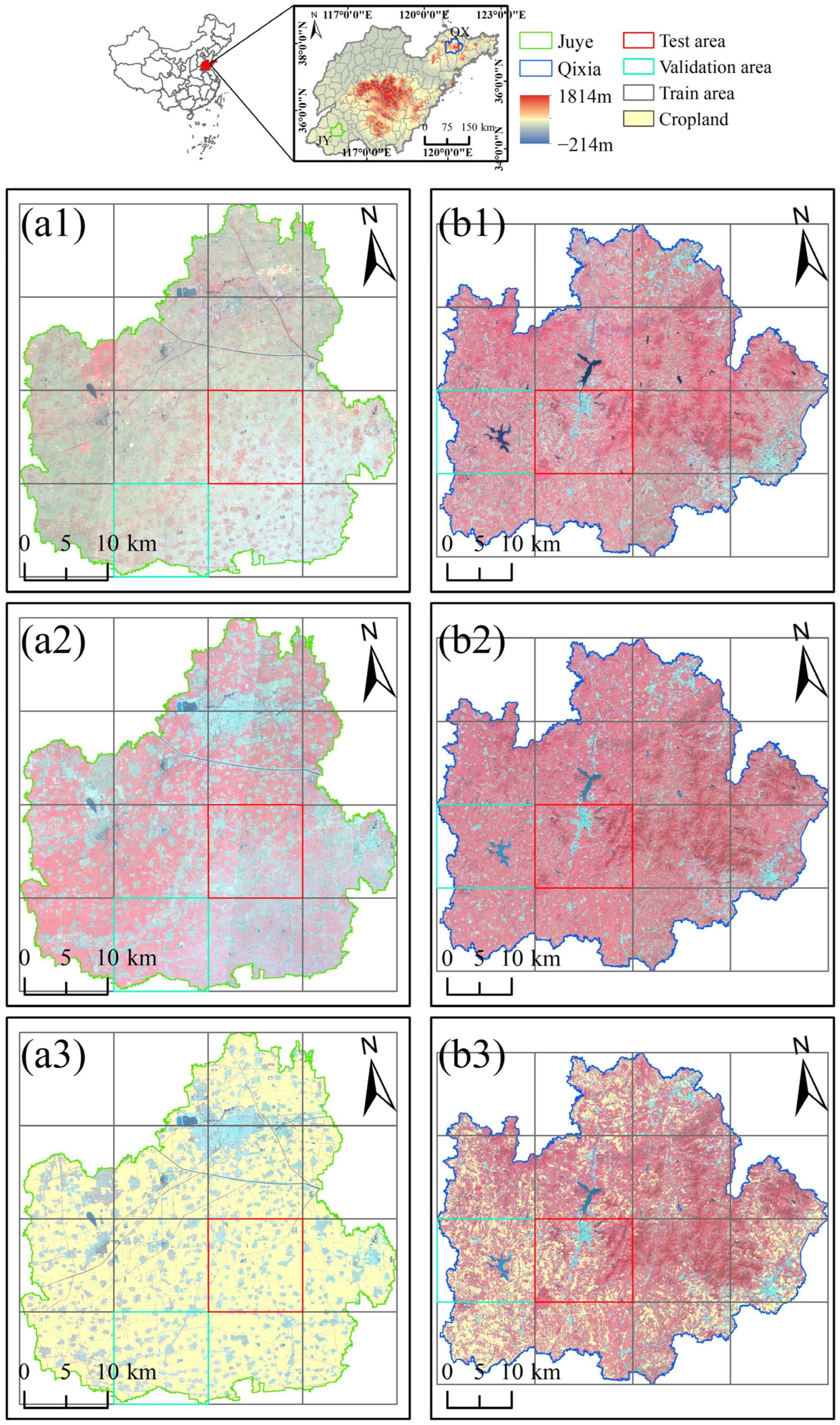
Figure 1. Two study areas: (a) Juye (JY) and (b) Qixia (QX). Each study area is split into training, validation, and test sets. (a1,a2) denote GF-1 images captured at different crop growth stages in Juye. (a1) was acquired during the non-vigorous growth stage of the crops on 20 October 2015, while (a2) was acquired during the vigorous growth stage on 1 April 2016. Similarly, (b1,b2) in Qixia were acquired on 25 June 2016 and 22 August 2016, corresponding to the non-vigorous and vigorous stages of the crops, respectively. (a3,b3) delineate the ground truth results of cropland covering the two study areas.
Land 14 02038 g001
Figure 2. Representative examples of cropland and non-cropland across various crop growth stages in Juye and Qixia.
Land 14 02038 g002
Figure 3. Two DL architectures employed in this study: (a) UNet and (b) DeepLabv3+. The dimensions of the feature maps per layer are in brackets, where the first number indicates the number of feature maps, while the second and third represent spatial dimensions.
Land 14 02038 g003
Figure 4. Three different mislabeling types. Over-labeling error represents instances where non-cropland pixels in the mislabeled grid tiles are mislabeled as cropland. Under-labeling error arises when the cropland pixels are mislabeled as non-cropland. Mix-labeling error occurs when cropland pixels are reassigned as non-cropland and simultaneously non-cropland pixels are mislabeled as cropland.
Land 14 02038 g004
Figure 5. Performance evaluation of UNet, DeepLabv3+, and OBIA-RF models with three band combinations across two different crop growth periods for high-resolution cropland extraction in Juye and Qixia. JY-T1 and JY-T2 refer to the non-vigorous and vigorous crop growth periods in Juye, respectively. Similarly, QX-T1 and QX-T2 refer to the non-vigorous and vigorous crop growth periods in Qixia, respectively. ALL means the Near-Infrared–Red–Green–Blue band combination, NRG means the Near-Infrared–Red–Green band combination, and RGB means the Red–Green–Blue band combination.
Land 14 02038 g005
Figure 6. Performance differences between the vigorous and non-vigorous crop growth periods (vigorous minus non-vigorous) for the three band combinations under three classifiers in Juye (JY) and Qixia (QX). ALL means the Near-Infrared–Red–Green–Blue band combination, NRG means the Near-Infrared–Red–Green band combination, and RGB means the Red–Green–Blue band combination.
Land 14 02038 g006
Figure 7. HRRS cropland extraction accuracies under different class mislabeling types and ratios. (ac) UNet, DeepLabv3+ and OBIA-RF results in Juye, respectively; (df) UNet, DeepLabv3+ and OBIA-RF results in Qixia, respectively. The X-axis presents the error area ratio, which is the ratio of mislabeled to total pixels and corresponds to the results in Table 4.
Land 14 02038 g007
Figure 8. HRRS cropland extraction accuracies under different patch sizes of sample blocks for UNet and DeepLabv3+ in Juye (JY) and Qixia (QX).
Land 14 02038 g008
Figure 9. HRRS cropland extraction accuracies of UNet, DeepLabv3+ and OBIA_RF models using the mixed and individual training sample datasets in Juye (JY) and Qixia (QX). ID means individual training sample datasets, containing only the individual agricultural landscape and crop growth stage. MD means mixed training sample dataset, containing all training data from the plain area Juye and the mountainous area Qixia in the vigorous and non-vigorous crop growth periods.
Land 14 02038 g009
Figure 10. HRRS cropland extraction accuracies of UNet and DeepLabv3+ models under different depths of the ResNet backbone architecture: ResNet18, ResNet34, ResNet50, ResNet101, and ResNet152.
Land 14 02038 g010
Table 1. Specifications for GF1 PMS data.
Launch TimeGlobal Observation
Cycle
Repeat Observation
Cycle
Swath Width (km)Spatial Resolution (m)Wavelength (nm)
26 April 201341 days4 days60PAN: 2
MS: 8
PAN: 450–900
Blue: 450–520
Green: 520–590
Red: 630–690
Infrared: 770–890
Table 2. The GF-1 images used in this study.
Study AreaTerrain CharacteristicCoverage (km2)Satellite SensorAcquisition Date
JuyePlain area1302GF-120 October 2015 (T1)
1 April 2016 (T2)
QixiaMountainous area1793GF-125 June 2016 (T1)
22 August 2016 (T2)
Table 3. HRRS cropland extraction accuracies of UNet, DeepLabv3+, and OBIA-RF models with three band combinations across two different crop growth periods for high-resolution cropland extraction in Juye and Qixia. JY-T1 and JY-T2 refer to the non-vigorous and vigorous crop growth periods in Juye, respectively. Similarly, QX-T1 and QX-T2 refer to the non-vigorous and vigorous crop growth periods in Qixia, respectively. ALL means the Near-Infrared–Red–Green–Blue band combination, NRG means the Near-Infrared–Red–Green band combination, and RGB means the Red–Green–Blue band combi-nation.
UNetDeepLabv3+_OBIA-RF
JY-T1ALLOA95.92%95.93%93.72%
Kappa88.11%88.13%82.45%
F1-score97.38%97.39%95.90%
PA98.21%98.26%95.09%
UA96.57%96.54%96.73%
NRGOA96.21%96.20%93.81%
Kappa88.99%88.95%82.56%
F1-score97.57%97.57%95.98%
PA98.28%98.39%95.52%
UA96.86%96.75%96.45%
RGBOA96.10%96.12%93.08%
Kappa88.89%88.76%80.80%
F1-score97.48%97.50%95.48%
PA97.49%98.10%94.39%
UA97.47%96.92%96.59%
JY-T2ALLOA96.26%96.38%95.10%
Kappa89.07%89.50%86.15%
F1-score97.60%97.68%96.82%
PA98.54%98.39%96.48%
UA96.68%96.98%97.16%
NRGOA96.78%96.68%95.14%
Kappa90.74%90.37%86.24%
F1-score97.93%97.87%96.85%
PA98.28%98.54%96.57%
UA97.57%97.21%97.13%
RGBOA96.60%96.66%93.28%
Kappa90.25%90.37%80.80%
F1-score97.80%97.85%95.66%
PA98.00%98.34%95.77%
UA97.61%97.37%95.55%
QX-T1ALLOA88.90%89.14%87.17%
Kappa63.40%63.68%51.95%
F1-score70.21%70.32%59.27%
PA70.21%69.07%50.12%
UA70.25%71.64%72.50%
NRGOA89.56%89.79%86.85%
Kappa64.76%65.30%50.13%
F1-score71.12%71.51%57.53%
PA69.07%68.77%47.81%
UA73.43%74.49%72.21%
RGBOA89.57%89.71%86.65%
Kappa64.83%64.87%49.05%
F1-score71.20%71.11%56.50%
PA69.25%67.99%46.54%
UA73.29%74.56%71.90%
QX-T2ALLOA87.98%88.41%84.86%
Kappa59.67%59.77%36.38%
F1-score67.00%66.75%43.65%
PA65.60%62.50%31.49%
UA68.81%71.74%71.11%
NRGOA88.70%88.90%84.70%
Kappa61.13%61.58%35.13%
F1-score67.97%68.27%42.33%
PA64.41%64.09%30.14%
UA71.99%73.04%71.06%
RGBOA88.49%88.98%84.45%
Kappa61.60%61.27%33.98%
F1-score68.64%67.86%41.27%
PA67.63%62.46%29.32%
UA69.77%74.34%69.62%
Table 4. Error area ratios under different noise levels and mislabeling types in the two study areas.
Error TypeNoise Level
IIIIIIIVVVIVII
Juye
Over-labeling0.0030.0160.0310.0610.0920.1240.154
Under-labeling0.0070.0340.0690.1390.2080.2760.346
Mix-labeling0.0100.0500.1000.2000.3000.4000.500
Qixia
Over-labeling0.0080.0410.0820.1640.2450.3260.408
Under-labeling0.0020.0090.0180.0360.0550.0740.092
Mix-labeling0.0100.0500.1000.2000.3000.4000.500
Table 5. HRRS cropland extraction accuracies of UNet and DeepLabv3+ models before and after data augmentation. OD denotes the original dataset without data augmentation. AD denotes the augmented dataset.
UNet_ODUNet_ADDeepLabv3+_ODDeepLabv3+_AD
JuyeOA96.60%96.72%96.66%96.85%
Kappa90.25%90.61%90.37%90.96%
F1-score97.80%97.88%97.85%97.97%
PA98.00%98.01%98.34%98.25%
UA97.61%97.75%97.37%97.70%
QixiaOA89.57%89.36%89.71%89.49%
Kappa64.83%64.17%64.87%64.23%
F1-score71.20%70.66%71.11%70.61%
PA69.25%68.83%67.99%67.75%
UA73.29%72.67%74.56%73.74%
Table 6. Comparison of computational times amongst OBIA-RF, UNet and DeepLabv3+.
Study AreaComputation Time (h)
OBIA-RFUNetDeepLabv3+
TrainJuye0.384.574.71
Qixia0.887.768.00
InferenceJuye0.010.030.04
Qixia0.020.040.05
Disclaimer/Publisher’s Note: The statements, opinions and data contained in all publications are solely those of the individual author(s) and contributor(s) and not of MDPI and/or the editor(s). MDPI and/or the editor(s) disclaim responsibility for any injury to people or property resulting from any ideas, methods, instructions or products referred to in the content.