Article

Vegetation Classification and Extraction of Urban Green Spaces Within the Fifth Ring Road of Beijing Based on YOLO v8

1
Institute of Forestry and Pomology, Beijing Academy of Agriculture and Forestry Sciences, Beijing 100093, China
2
Beijing Yanshan Forest Ecosystem Research Station, National Forest and Grassland Administration, Beijing 100093, China
3
College of Forestry, Shenyang Agricultural University, Shenyang 110866, China
4
Remote Sensing Application Center, China Academy of Urban Planning & Design, Beijing 100835, China
5
Institute of Environment and Sustainable Development in Agriculture, Chinese Academy of Agricultural Sciences, Beijing 100093, China
*
Authors to whom correspondence should be addressed.
These authors contributed equally to this work.
Land 2025, 14(10), 2005; https://doi.org/10.3390/land14102005
Submission received: 21 August 2025 / Revised: 28 September 2025 / Accepted: 29 September 2025 / Published: 6 October 2025
(This article belongs to the Special Issue Vegetation Cover Changes Monitoring Using Remote Sensing Data)

Abstract

Real-time, accurate and detailed monitoring of urban green space is of great significance for constructing the urban ecological environment and maximizing ecological benefits. Although high-resolution remote sensing technology provides rich ground object information, it also makes the surface information of urban green spaces more complex. Existing classification methods often struggle to meet the requirements of classification accuracy and the automation demands of high-resolution images. This study utilized GF-7 remote sensing imagery to construct an urban green space classification method for Beijing. The study used the YOLO v8 model as the framework to conduct a fine classification of urban green spaces within the Fifth Ring Road of Beijing, distinguishing between evergreen trees, deciduous trees, shrubs and grasslands. The aims were to address the limitations of insufficient model fit and coarse-grained classifications in existing studies, and to improve vegetation extraction accuracy for green spaces in northern temperate cities (with Beijing as a typical example). The results show that the overall classification accuracy of the trained YOLO v8 model is 89.60%, which is 25.3% and 28.8% higher than that of traditional machine learning methods such as Maximum Likelihood and Support Vector Machine, respectively. The model achieved extraction accuracies of 92.92%, 93.40%, 87.67%, and 93.34% for evergreen trees, deciduous trees, shrubs, and grasslands, respectively. This result confirms that the combination of deep learning and high-resolution remote sensing images can effectively enhance the classification extraction of urban green space vegetation, providing technical support and data guarantees for the refined management of green spaces and “garden cities” in megacities such as Beijing.

1. Introduction

Urban green space vegetation classification and extraction provide not only a basic understanding of green space, but also a critical “data foundation” for achieving urban ecological protection, spatial optimization, and the improvement of people’s livelihoods. It transforms fragmented green space information into systematic knowledge, offering a scientific basis for transforming cities from “extensive development” to “refined governance”. The study defines “green space” as vegetation, primarily that which serves the purposes of urban ecological improvement, environmental protection, recreational areas for residents, and urban beautification, with further boundaries. Specifically, it refers to artificially cultivated or semi-artificial green spaces within Beijing’s Fifth Ring Road, which are predominantly composed of woody plants (trees and shrubs) and herbaceous vegetation. It is classified according to the vegetation life type and morphological characteristics: trees (evergreen trees, deciduous trees) and shrubs, herbs (grassland), which meet the practical needs of “easy identification and easy quantification” in urban green space monitoring. Early remote sensing for urban green space info mainly used visual interpretation: operators identified green space types via image patch features (shape, color, texture) based on experience, with accuracy relying on their target familiarity. For unfamiliar areas, other data were needed. The process was time-consuming, could not process data in batches, and its timeliness/convenience failed to meet requirements [1,2].
Within urban areas, green spaces show significant differences in spectral characteristics compared to other features. Urban green spaces can be distinguished from other features through inter-band computation and fusion methods to extract urban green space data [3]. To reduce the influence of factors such as the surrounding environment of urban green spaces, similar features, and building shadows on extraction results, some scholars, using inter-band operations, optimized band combination strategies and proposed vegetation indices such as the Normalized Difference Vegetation Index (NDVI) for extracting urban green space information [4,5]. However, in complex urban environments, there is a strong interrelationship between urban green spaces and other features, and their spectral characteristics can be easily influenced by other features, making it impossible to finely identify urban green spaces using vegetation indices [6]. Xu used the YOLO v7 network to carry out iterative parameter training on the training set and obtained the optimal parameters to output the information of a single tree type. The peak accuracy rate of single tree species recognition reached 85.42%, but, due to the lack of data enhancement, the classification accuracy rate of the model was limited in the face of a complex forest canopy area [7]. To address the limitations of traditional object detection models in small target detection, Khalili’s research team developed the SOD-YOLOv8 model. While building upon YOLOv8 with an enhanced backbone network architecture, this approach still has limitations. Specifically, in green space vegetation classification, the model focuses solely on improving small target detection accuracy without differentiating between “evergreen and deciduous trees.” Consequently, it fails to provide comprehensive data support for seasonal monitoring and precision management of urban green spaces [8].
With the development of machine learning technology, an increasing number of machine learning algorithms have been applied to urban green space extraction, including Support Vector Machine (SVM), Maximum Likelihood Classification (MLC), and Random Forest (RF) [9]. These methods require the creation of a study area sample dataset for subsequent data analysis. Noi & Kapps compared the performance of different machine learning algorithms in identifying urban green spaces using Sentinel-2 remote sensing imagery. They found that different machine learning algorithms have varying requirements for sample size, but when the sample size reaches a certain proportion of the study area, all algorithms show higher overall classification accuracy [10].
Deep learning constitutes a deep neural network algorithm and is one of the branches of machine learning, evolving from artificial neural networks [11]. Compared with traditional machine learning, deep learning can automatically obtain complex nonlinear relationships between different features such as spectra, textures, and shapes in remote sensing images. Through weight learning across multi-layer networks, deep learning avoids the need for manual feature selection. Its hierarchical network structure can extract green space features nonlinearly at different levels, showing stronger generalization abilities [12]. Compared with other machine learning methods, deep learning has shown greater advantages in classification and recognition tasks, providing a new solution for extracting urban green space information from satellite remote sensing data; it has been increasingly applied to high-resolution data [13,14]. The innovation of this study, “YOLOv8 + data enhancement + four categories of subdivision”, is not only suitable for the vegetation characteristics of northern temperate cities (such as seasonal changes of deciduous trees) but also solves the problem of small target detection leakage.
As one of the classic network architectures of deep learning, Convolutional Neural Networks (CNNs) have become the mainstream algorithm for extracting information from remote sensing data, owing to their efficient feature extraction capabilities [15]. Semantic segmentation models based on CNNs can achieve pixel-level category recognition in images and automatically extract greenfield information against complex backgrounds [16]. Liu first applied the DeepLabv3+ semantic segmentation network to extract urban green spaces from GF-2 satellite images. The results showed that the overall classification accuracy of green spaces in cities such as Guangzhou was 91.02%, outperforming traditional machine learning methods. Meanwhile, the deep learning YOLO v8 model performed better in localizing and extracting small targets, achieving an average recognition accuracy of 95.11% across various object and ground types in the ROSD dataset [17]. As the performance of deep learning models continues to improve, researchers have begun applying them for the extraction of green space information on a large scale and in multiple cities. For example, Shi used deep learning models to analyze, extract and map green space information across 31 major cities in China [18].
Beijing, a megacity, has heterogeneous, fragmented green space vegetation (mixed trees, shrubs, etc.) [19] and blurred green space-artificial feature boundaries due to urbanization. Existing studies have largely lacked specialized extraction for the specific types of green spaces in Beijing, highlighting the urgent need for more adaptable technical tools. YOLO v8’s high precision in small target localization/extraction effectively identifies scattered small vegetation units, fixing traditional semantic segmentation models’ flaw of missing/misclassifying small targets [20,21]. Its end-to-end framework directly outputs vegetation category and bounding box info (no extra post-processing), achieves “classification + location” simultaneously, and fits Beijing’s green space extraction needs of complex types and ambiguous boundaries.
While previous studies have verified the effectiveness of deep learning in green space extraction, two limitations remain for application in Beijing: (1) insufficient model fit; and (2) the existing studies mostly focus on the binary division of “green space/non-green space”. In view of this, this study conducted vegetation classification extraction of urban green spaces within the Fifth Ring Road in Beijing using the YOLO v8 algorithm. The main objectives include: (1) to systematically explore the adaptability and accuracy of YOLO v8 in northern temperate cities, using Beijing as a typical example; and (2) to verify whether high-resolution satellite images and the YOLO v8 model can achieve the fine-scale classification of vegetation in Beijing’s green spaces, such as distinguishing evergreen trees, deciduous trees, shrubs and grasslands and providing a data basis for differentiated management. This study not only responds to the specific green space characteristics and management requirements of Beijing but also represents an important advancement in applying deep learning technologies to urban ecological monitoring, and its results can provide key technical methods and data support for “Beijing Garden City”.

2. Materials and Methods

2.1. Study Area

Beijing is located between 115°25′ and 117°30′ east longitude and 39°28′ and 41°25′ north latitude, covering a total area of approximately 16,410 km2. Since the implementation of the reform and opening up policy in 1978, Beijing has experienced rapid social and economic development, with a rapid expansion of the city and a significant increase in the construction of urban green spaces. The Fifth Ring Road of Beijing is defined as the study area, with a total area of 666.5 km2. The urban green spaces within the Fifth Ring Road primarily consist of small- and medium-sized patches with diverse vegetation types.

2.2. Data Sources and Data Processing

2.2.1. Satellite Images

GF-7 provides high-resolution panchromatic stereoscopic images and 4-band multispectral images, with spatial resolutions of 0.8 m and 3.2 m, respectively, which can effectively cover a width of 20 km. This study used 4 scenes of GF-7 image data acquired between April and October 2024 (http://eds.ceode.ac.cn/nuds/businessdataquery, accessed on 1 April 2024). Each scene includes a multispectral image and two panchromatic images.

2.2.2. Data Processing

Building on high-resolution remote sensing data from the GF-7 satellite, we developed a Beijing urban green space classification framework using the YOLO v8 model. This refined classification system for green spaces within Beijing’s Fifth Ring Road integrates field surveys with manual interpretation, addressing limitations in existing studies such as inadequate model adaptability and coarse classification granularity. The approach significantly enhances vegetation extraction accuracy in northern temperate cities (with Beijing as a representative case). Throughout this study, we utilized the YOLO v8 deep learning model to annotate 1130 sample images and implement data augmentation techniques.
(1) Multispectral image preprocessing
First, orthographic and geometric corrections were applied to the original images, followed by image registration with the Tiandi map. Atmospheric correction was then applied to the registration results in order to obtain the real surface reflectance data. Based on this, multispectral band data and panchromatic band data were fused to generate 4-band GF-7 multispectral image data with a resolution of 0.65 m. Finally, using image stitching and mosaicking techniques, the four generated images were combined into a 0.65 m resolution multispectral image covering the entire study area (Figure 1).
(2) Training and validating images
Extracting urban green space information based on the YOLO v8 deep learning framework requires a high-quality sample dataset for model training. Training samples were created through a combination of field investigation and human interpretation, where the accuracy of sample labels directly affects the classification performance of the model. In this study, the training sample divided urban green spaces into four categories: evergreen trees, deciduous trees, shrubs, and grasslands.
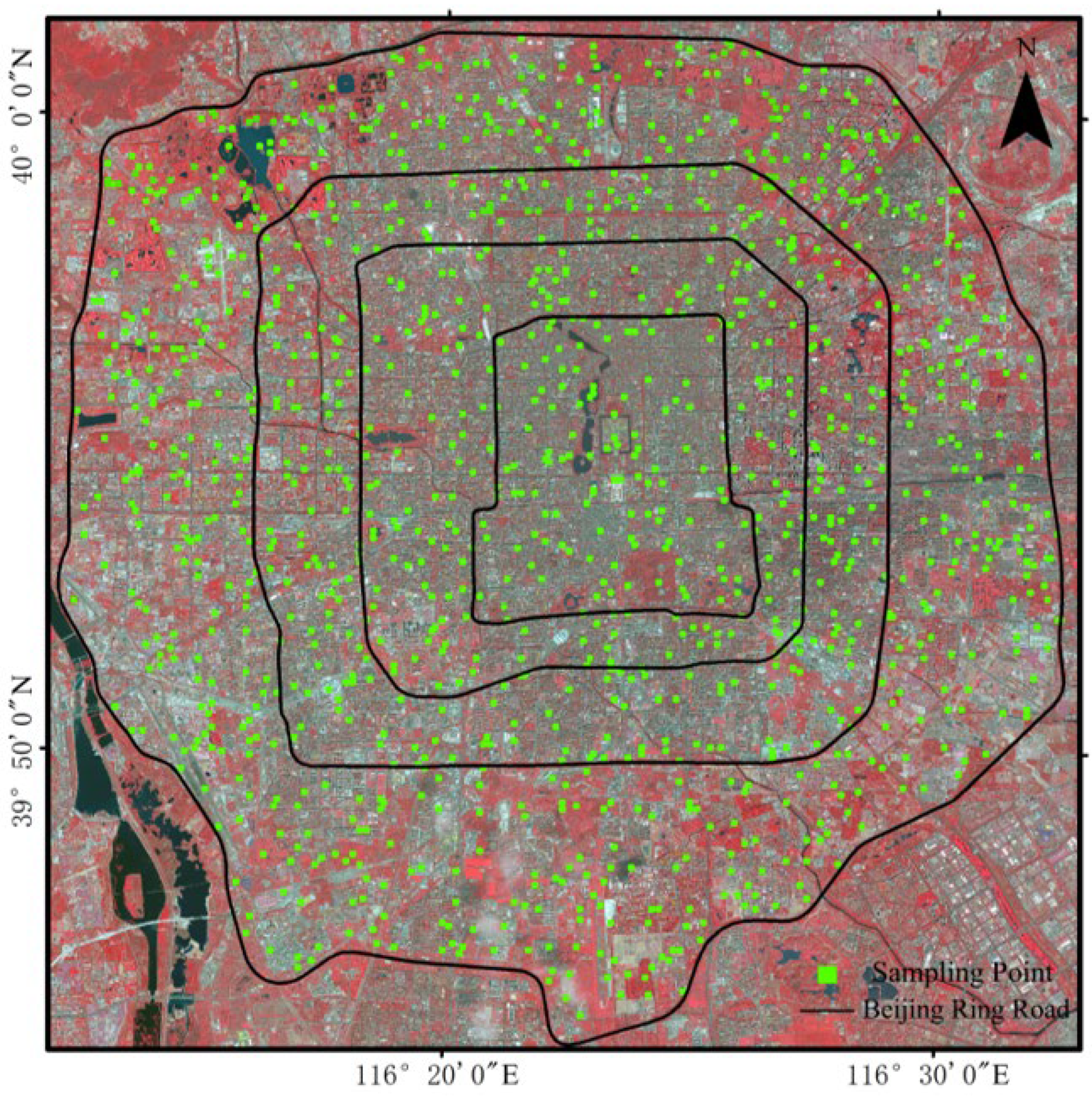
Based on the spectral characteristics of vegetation with significant reflection properties in the near-infrared band, pseudo-color images were generated using band combinations as supplementary data for the sample set construction process. Field survey data were then used to refine the sample labels. Using the feature of generating random points in ArcGIS 10.7, a total of 1130 random points were generated within the Fifth Ring Road of Beijing. Deep learning model YOLO v8 segmented image training samples of basic standard size 512 pixels × 512 pixels. In this study, 1130 sample images were selected according to the proportion of sub-scenarios (19% of evergreen trees, 49% of deciduous trees, 15% of shrubs, and 17% of grasslands) and annotated to ensure that the sample proportion of each sub-scenario matched the area/importance of the sub-scenario in the actual urban area (see Figure 2). The “statistical power analysis” G*Power 4 calculation proves that 1130 samples can meet the statistical test requirements of this study under α = 0.05 and β = 0.2, ensuring the statistical significance of the conclusions.
(3) Data augmentation
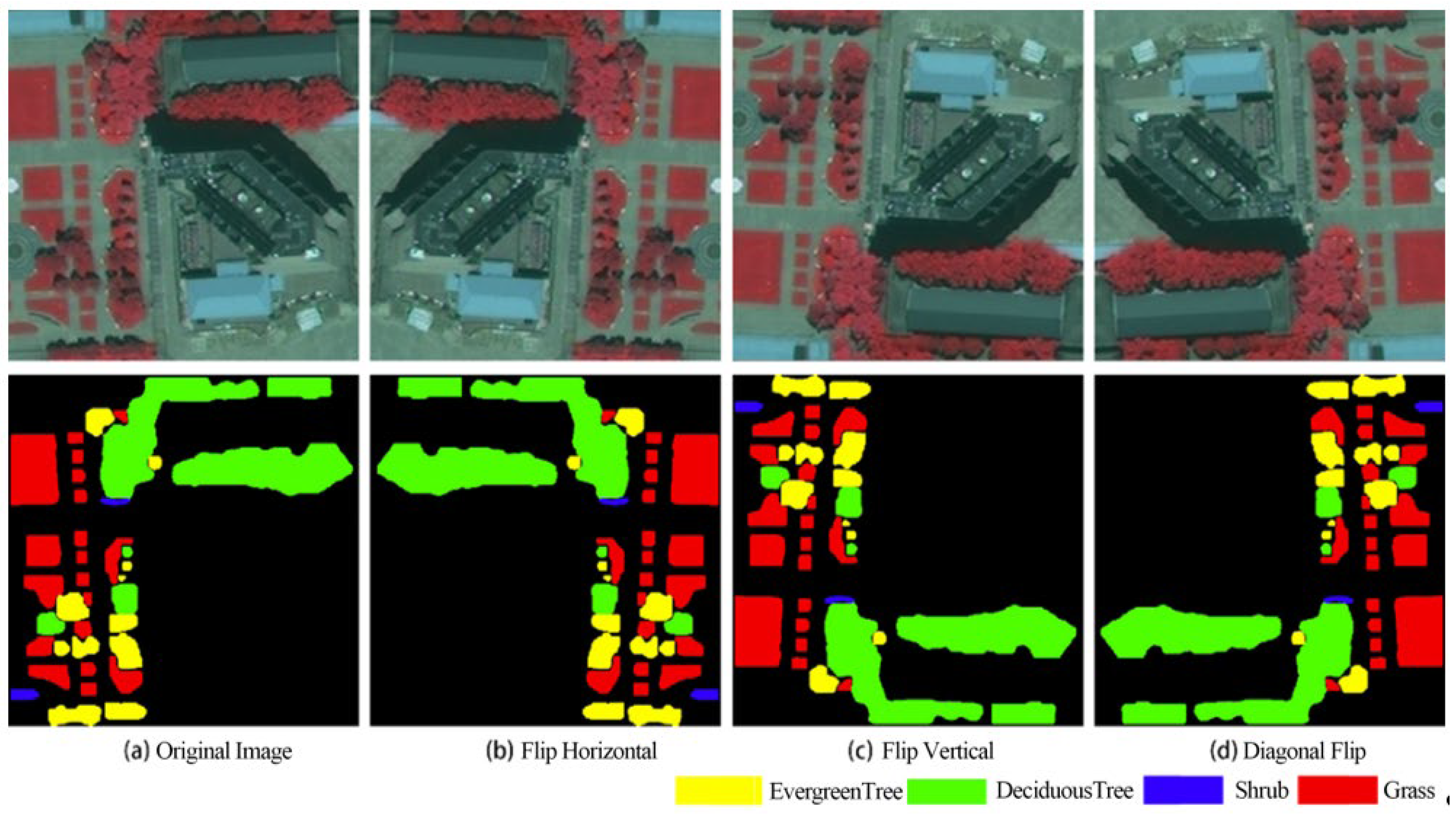
Due to the inherent limitations of visual interpretation methods, labeling large volumes of sample images has remained a challenge. Data augmentation is achieved by rotating the image at a certain angle to simulate different perspectives, translating the image horizontally or vertically to simulate positional changes, and enlarging or reducing the image to simulate distance changes. This method can effectively expand the dataset, enhance model generalization performance, and help prevent overfitting. In this study, all sample images were flipped in different directions for data augmentation. After processing, the sample dataset was expanded to four times its original size. Figure 3 shows a schematic diagram of the sample augmentation process.
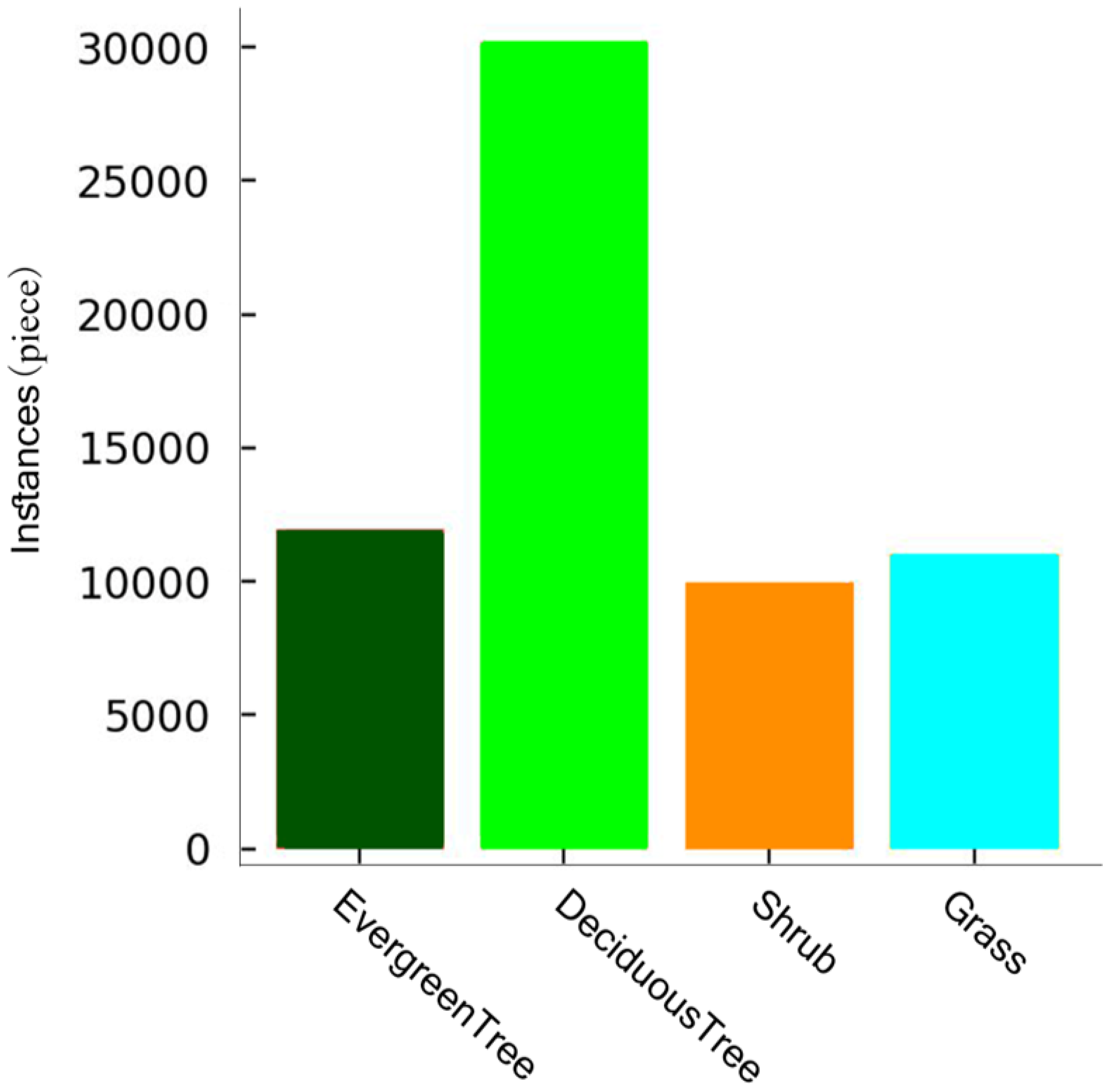
As shown in Figure 4, the sample set after data augmentation consists of 4520 samples, with a total of 79,044 elements (Figure 4). Following the construction of the sample, 80% of the sample set was randomly selected as the training set, while the remaining 20% was used as the validation set.

2.3. Methods

2.3.1. YOLO v8 Deep Learning Model

YOLO v8 is a 2023 object detection model developed by Ultralytics. Unlike prior YOLO versions, it uses an optimized backbone network (extracts high-level image features via convolution) and an improved feature pyramid structure (multi-scale classification). Fusing different-level feature maps allows it to keep high accuracy for both large and small object detection [22,23]. YOLO v8’s instance segmentation adopts a single-stage end-to-end (Backbone–Neck–Head) architecture, centered on “shared features + dynamic masks”. Backbone extracts, Neck fuses multi-scale features, and Head outputs info to generate masks. Trained with multi-task loss, it uses NMS in inference to obtain “box-category-mask” triplets, balancing speed and accuracy.
Unlike traditional object detection models, YOLO v8 uses a regression-based method to directly predict object categories from image pixels, with no extra candidate region generation needed [24]. It turns detection into a regression problem via a single neural network for end-to-end training, which auto-optimizes network parameters, letting the model learn from large datasets and improve detection/classification capabilities [25]. Ahmed used YOLOv8 to classify Karachi Green in Pakistan, with an overall accuracy of 88.2%, but only classified “green/non-green” without subdividing vegetation types [26]. Chen used the YOLOv8 + GF-2image classification of Shanghai green land with an accuracy of 87.5%, but this did not involve deciduous tree recognition, because Shanghai has a subtropical climate (vegetation is evergreen all year round) [27]. Yan used YOLOv8 to classify shrubs in UAV images with a recall rate of 85%, but the coverage range of UAV images is small (less than 1 km2 per image), meaning that it cannot be adapted to the large-scale extraction of Beijing’s Fifth Ring Road (666.5 km2) [28].

2.3.2. Support Vector Machine

SVM’s core premise is to find the optimal classification hyperplane in feature space via structural risk minimization. It maps input features to high-dimensional space with nonlinear functions and then builds a hyperplane maximizing sample intervals for linear separability. It is independent of data distribution assumptions, handles nonlinear problems via kernel functions, with support vectors (samples closest to the hyperplane) determining boundaries; it also boosts nonlinear classification and generalization [29].

2.3.3. Maximum Likelihood Classification

MLC assumes that each data category follows a specific probability distribution. It assigns each sample to the category with the highest probability value by calculating the posterior probability that it belongs to each category. The advantage of this method lies in the well-developed theoretical system. However, its classification performance is highly dependent on data distribution assumptions, making it difficult to handle nonlinear problems. The method also places high demands on the quantity and quality of training samples, is prone to overfitting in the case of small samples, and is sensitive to noise. Additionally, the presence of outliers can interfere with the classification process, thereby reducing the accuracy of the classification results [30].

2.3.4. Evaluation Metrics

To assess the validity of the model, the accuracy of the urban green space classification results was evaluated using a confusion matrix. The confusion matrix compares the classification results with the true values of the samples and calculates several key performance metrics: Overall Classification Accuracy (OA), the Kappa Coefficient, User Accuracy (UA) and Producer Accuracy (PA). These indicators help analyze the classification performance across different categories. At the same time, the F1 score indicator was introduced to evaluate the classification effectiveness of the model. The calculation formulas are shown in Table 1.

3. Results

3.1. Training of Deep Learning Models

Based on the construction of the deep learning model training sample set, the model is trained using the YOLO v8x-seg.pt base model weights. During the training process, YOLO v8 automatically optimizes and dynamically adjusts key network parameters—such as the learning rate—to optimize model performance and improve the segmentation accuracy of fine-scale features. The model was configured with four segmentation categories, the number of training iterations was set to 100, the batch size to 16, an initial learning rate to 4 × 10⁻³, and an early stop wait round to 20. The model was completed in the Python 3.12 framework.
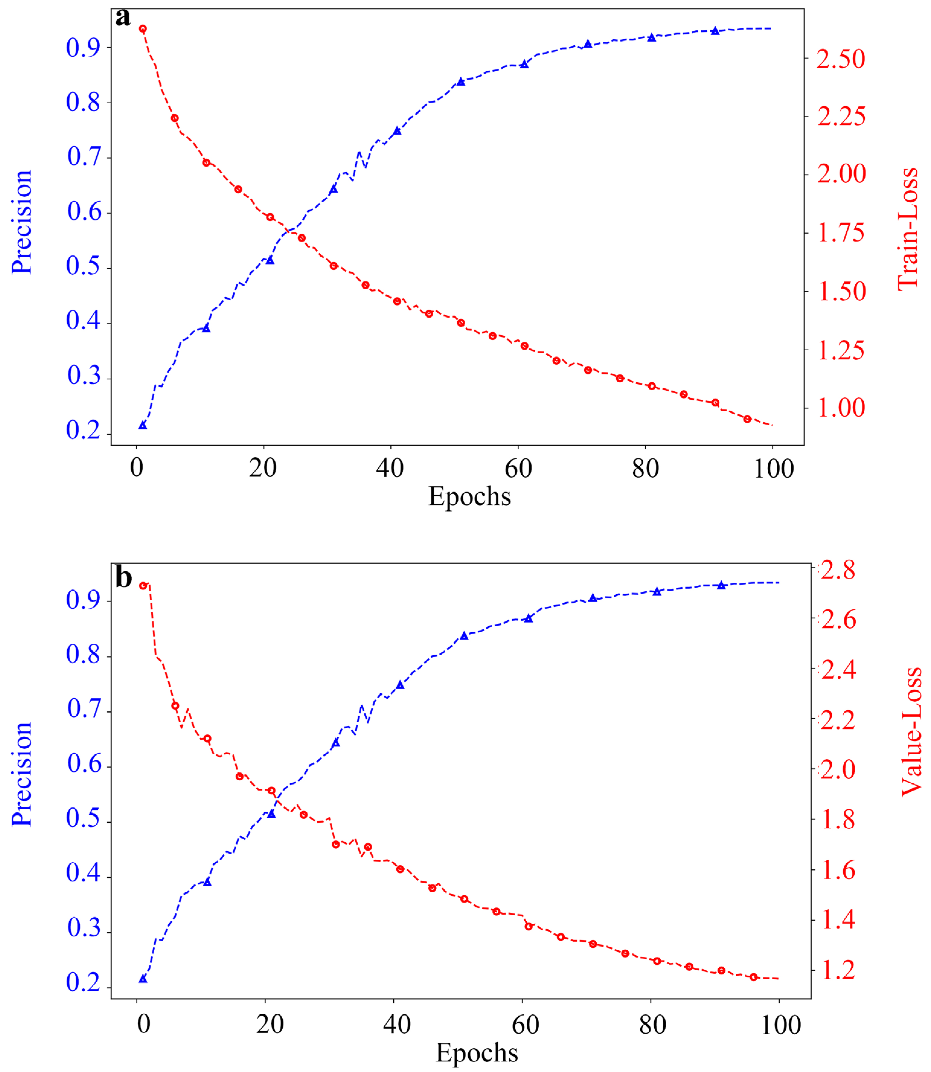
Figure 5 shows the training curves for accuracy and loss of the YOLO v8 deep learning model. The model reached its optimal performance after 100 rounds of training, at which point the training was stopped. Figure 5a shows that the classification accuracy of the model increases rapidly in the first 40 rounds, after which the growth rate gradually stabilizes. Figure 5b shows that the loss value of the training set drops sharply in the first 30 rounds of training, followed by a significant decline that eventually converges to around 0.8. Meanwhile, the loss value of the validation set gradually approaches 1.1. The smoothness of the training curve and the small fluctuation range suggest that the learning rate is appropriately configured. The fast convergence of the loss function confirms the effective learning ability of the network on the training samples. The absence of loss rebound and signs of overfitting indicates that the model achieves the expected training effect.

3.2. Accuracy Evaluation of the Green Space Classification Model Within the Five Rings

3.2.1. Comparison of Model Classification Accuracy

By constructing a confusion matrix, the classification prediction results of the three methods were compared and verified with the true value data. Four metrics—UA, PA, OA, and the Kappa Coefficient—were calculated to measure the accuracy of the extracted classification results.
As shown in Figure 6, the user accuracy of evergreen trees, deciduous trees, shrubs, and grasslands in the extraction results of the YOLO v8 deep learning model reached the highest values, which were 92.92%, 94.65%, 87.67%, and 93.34%, respectively. In the SVM extraction, the user accuracy of shrubs (81.47%) was higher than that of evergreen trees, deciduous trees and grasslands. In the MLC extraction, deciduous tree user accuracy (90.81%) reached the maximum value, while shrub user accuracy (47.95%) was the lowest, with the most severe misclassification.
As shown in Figure 7, the producer accuracy of evergreen trees, deciduous trees, shrubs, and grassland in the extraction results of the YOLO v8 deep learning model reached the highest values—89.92%, 93.40%, 85.60%, and 89.52%, respectively. In the SVM extraction results, the producer accuracy of deciduous trees was the highest at 82.94%, while shrubs had the lowest at 51.87%. In the MLC extraction results, the producer accuracy of evergreen trees reached the maximum at 78.29%, while that of shrubs was the lowest at 64.50%, with the highest missed detection rate.
The results show the study-trained YOLO v8 has excellent classification abilities (Table 2): overall accuracy 89.60%, Kappa 0.798, F1 0.860—all far better than traditional SVM and MLC. It efficiently extracts four green vegetation types with few misclassifications, low errors and high reliability. SVM (accuracy 71.53%) and MLC (69.57%) produce similarly low values (Kappa 0.52–0.55, F1 0.69–0.72, medium level). In summary, YOLO v8 significantly boosts classification consistency and accuracy compared to traditional methods, supporting the subsequent analysis.

3.2.2. Comparison of Model Classification Results

The same sample area was selected and classified using three trained models: the YOLO v8 deep learning model, the SVM model, and the MLC model. We analyzed the classification and extraction of four green vegetation types (evergreen trees, deciduous trees, shrubs, and grasslands) by the three different models. The classification accuracy of different algorithms for green vegetation types is shown in Table 3.
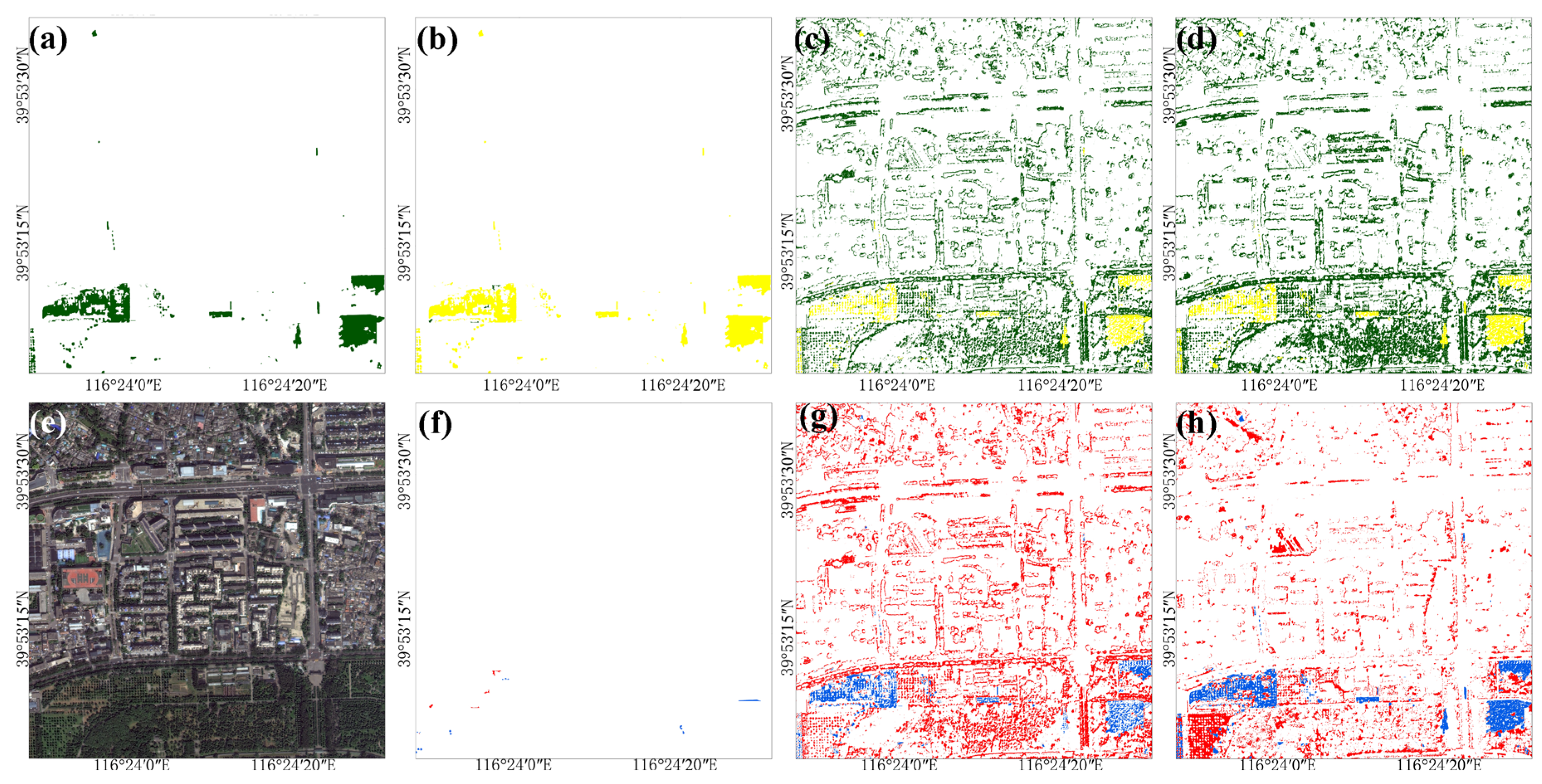
(1) Evergreen trees
Figure 8e is the sample area’s true-color image, and Figure 8a is the evergreen tree label image (green = true values). In Figure 8b–d, yellow denotes correct predictions of YOLO v8, SVM, and MLC sequentially; YOLO v8’s correct extraction rate (92.67%) is far better than those of SVM (46.27%) and MLC (61.14%). In Figure 8f–h, red represents misclassifications: SVM (437.92%) and MLC (262.89%) have severe misclassifications (SVM largest, uniformly distributed), while YOLO v8 (3.66%, concentrated in evergreen areas) is lowest. Blue represents missed extractions: MLC (82.51%) is much higher than SVM (53.83%) and YOLO v8 (4.35%).
In summary, the YOLO v8 model achieved the best recognition results for evergreen trees, with fewer incorrect extractions and omissions. Compared with SVM, MLC had a significantly smaller misclassification area but a larger omission area; though MLC identifies evergreen trees more accurately, it is more likely to miss relevant areas. Thus, the evergreen tree classification performance ranks as: YOLO v8 deep learning model > MLC model > SVM model.
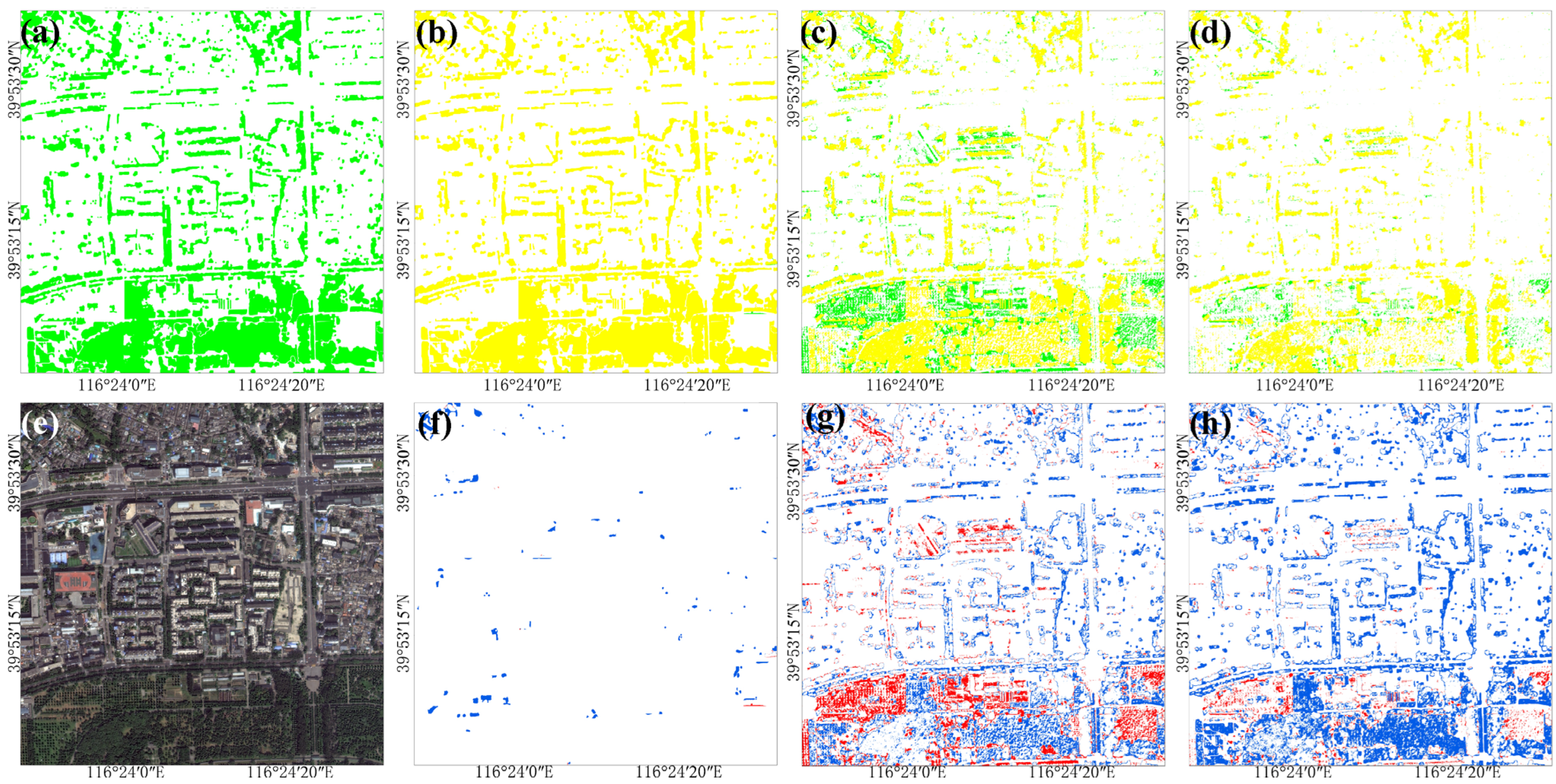
(2) Deciduous trees
Figure 9a is the deciduous tree label image of the sample area (green = true values). In Figure 9b–d, yellow denotes correct classifications of YOLO v8, SVM, MLC sequentially; YOLO v8’s correct extraction rate (95.69%) is far better than that of SVM (63.30%) and MLC (40.73%). In Figure 9f–h, red represents misclassifications: SVM’s misclassification rate (81.70%) is much higher than that of MLC (5.86%) and YOLO v8 (1.05%), with the largest area. Blue represents missed extractions: SVM (36.70%) and MLC (59.27%) have severe misses (MLC largest, concentrated), while YOLO v8 (3.02%) is lowest.
To sum up, the YOLO v8 model had the best recognition performance for deciduous trees, with significantly fewer errors and omissions than the other two models. Although MLC performed worse than SVM in terms of correct classifications and missed detections, it achieved a 75.84% reduction in misclassifications, enabling it to recognize deciduous tree information more accurately. Therefore, the classification performance of the deciduous tree model is as follows: YOLO v8 deep learning model > MLC model > SVM model.
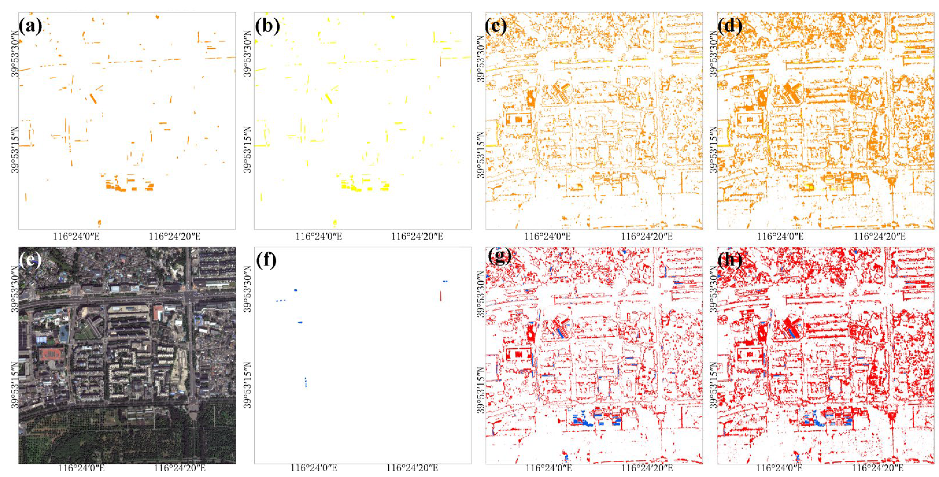
(3) Shrubs
Figure 10a is the sample area’s shrub label image (orange = true values). In Figure 10b–d, yellow denotes correct classifications of YOLO v8, SVM, and MLC sequentially; YOLO v8’s correct extraction rate (89.08%) is far better than those of SVM (25.27%) and MLC (47.88%). In Figure 10f–h, red represents misclassifications: SVM (899.4%) and MLC (1645.39%) have severe misclassifications (MLC largest, often mistaking buildings for shrubs), while YOLO v8 (4.38%) is lowest. Blue represents missed extractions: SVM’s omission rate (74.73%) is much higher than those of MLC (52.12%) and YOLO v8 (7.39%).
To sum up, the YOLO v8 model is the best for shrub identification, with the lowest rates of misclassification and omission. Compared with MLC, SVM has a lower area of correct classification and missed classification than MLC, but the area of misclassification of the SVM model is significantly reduced, and both models have poor recognition performance. The shrub model performs as follows: YOLO v8 deep learning model > SVM model ≈ MLC model.
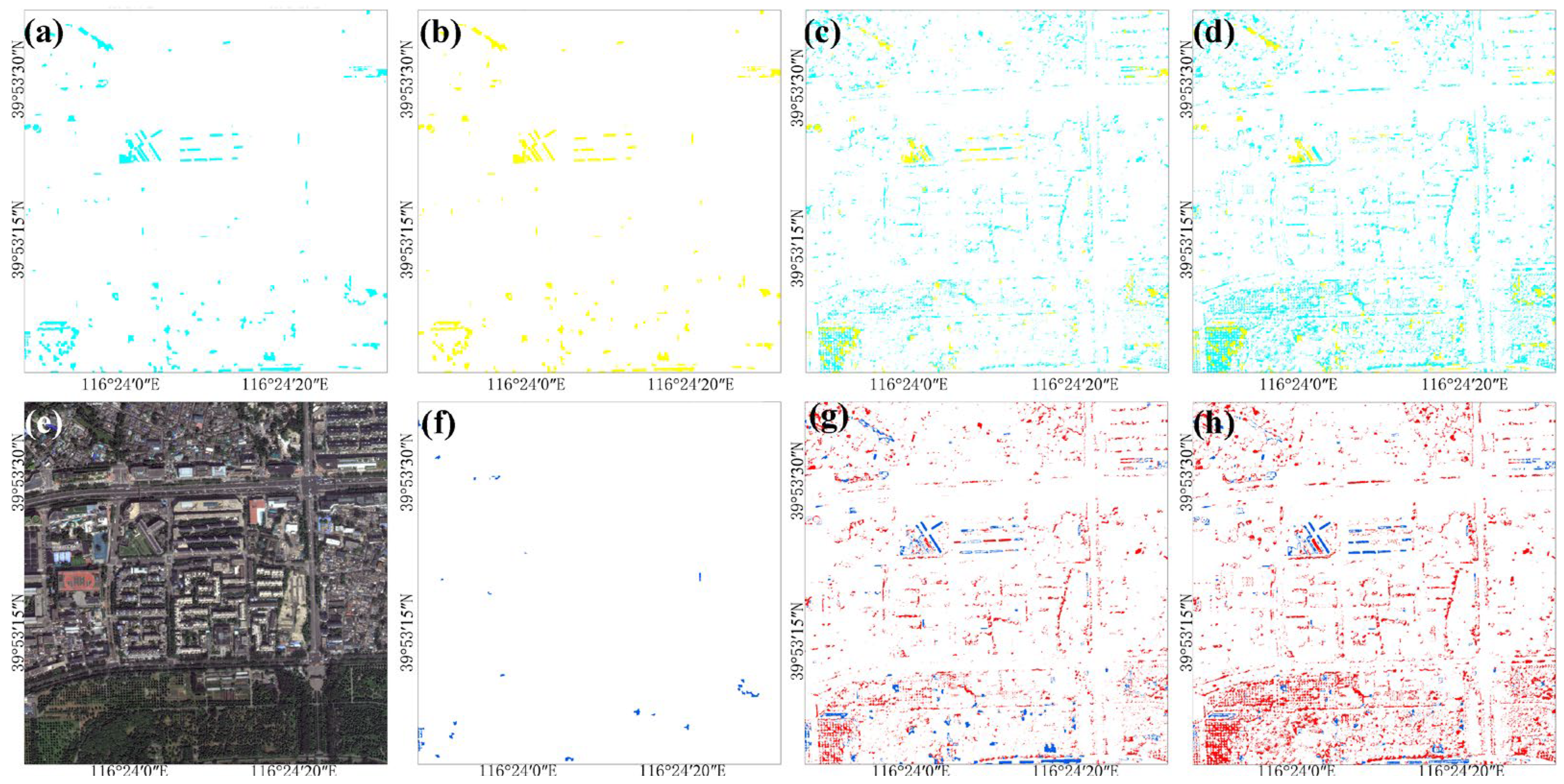
(4) Grassland
Figure 11a is the sample area’s grassland label image (cyan = true values). In Figure 11b–d, yellow denotes correct classifications of YOLO v8, SVM, and MLC sequentially; YOLO v8’s correct rate (89.06%) is far better than those of SVM (46.74%) and MLC (55.82%). In Figure 11f–h, red represents misclassifications: SVM (177.18%) and MLC (308.00%) have severe misclassifications (MLC largest, concentrated in dense vegetation), while YOLO v8 (1.54%) is lowest. Blue represents missed extractions: SVM (53.26%) and MLC (44.18%) have serious misses, with SVM having the largest missed area.
In summary, the YOLO v8 model performed best in grassland recognition, with fewer misclassifications and omissions. Compared with SVM, MLC correctly extracted more grassland areas; SVM had a smaller misclassification area but a larger missed detection area than MLC, making their grassland extraction performance comparable. MLC captures more grassland information but with more errors, while SVM is more accurate but prone to omissions. Thus, grassland classification performance ranks as follows: YOLO v8 deep learning model > SVM model ≈ MLC model.
Based on the sample area tests, the YOLO v8 deep learning model outperformed both SVM and MLC in extracting and classifying various vegetation types. It demonstrated the smallest misclassification and omission areas, along with greater stability. Therefore, the trained YOLO v8 deep learning model was selected to extract urban green space vegetation types across the study area for further analysis.

3.3. Spatial Analysis of Green Space Classification Within the Fifth Ring Road

(1) Spatial distribution of urban green spaces
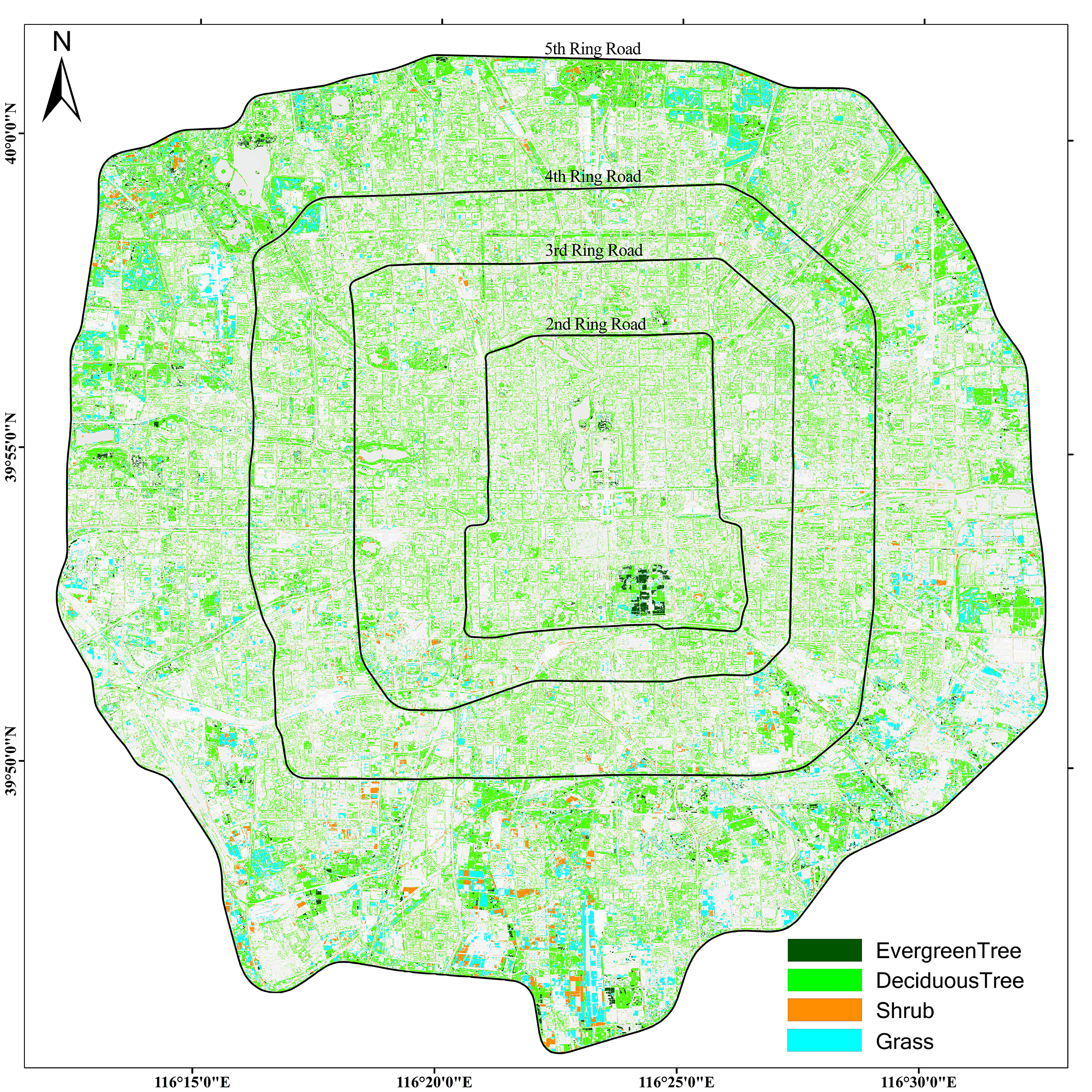
Figure 12 shows the classification extraction results of urban green spaces within the Fifth Ring Road in Beijing. The distribution of deciduous trees is relatively uniform, with larger clusters concentrated between the fourth and fifth rings. Evergreen trees are mainly distributed in parks within the Second Ring Road and within the fourth and fifth rings. Shrubs appear scattered around the second, fourth, and fifth rings, and they follow a lane distribution pattern. Grassy green spaces are mainly distributed in large parks and golf course areas along the fourth and fifth rings.
The information extracted by the ring of urban green spaces is shown in Table 4. The total area covered by evergreen trees in the study area is 6.23 km2. The largest proportion, 4.26 km2 (68.28%), is located between the fourth and fifth rings. The proportion of evergreen tree coverage within the second and third rings was the lowest, only 0.34 km2, accounting for 5.43%. The overall comparison shows that the evergreen tree coverage between the rings is as follows: fourth–fifth rings (4.26 km2) > second ring (0.89 km2) > third–fourth rings (0.74 km2) > second–third rings (0.34 km2).
(2) Evergreen trees
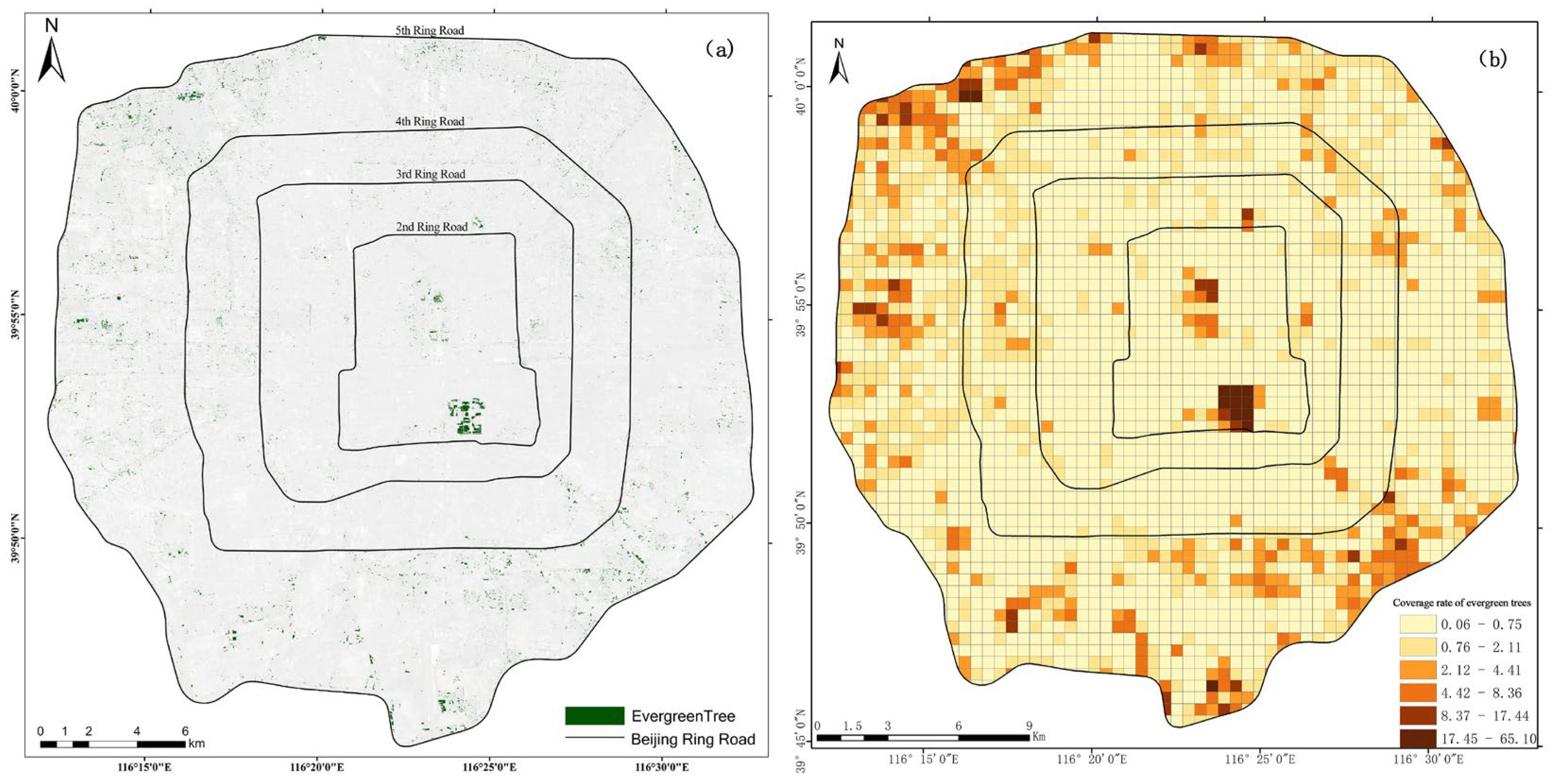
Figure 13a shows the overall distribution of evergreen tree green space vegetation in the study area. The distribution is generally scattered, with only the Second Ring Road’s parks showing a block-like distribution. The analysis shows that 0.25 km2 grids reflect green space vegetation spatial distribution more clearly than 1 km2 ones, so this study uses the former. Figure 13b (0.25 km2 grid) shows high evergreen tree coverage, mostly in the fourth to fifth rings, especially northwest and southeast (green space/park clusters).
Within Beijing’s Fifth Ring Road grids, evergreen tree coverage ranges from 0.06–65.10% (avg 1.15%), with only 25.46% of grids above average (most 0.06–1.15%). Darker colors in the figure mean higher coverage: the second to fourth rings have uniformly low coverage, while rings four to five have block-like high coverage (concentrated in green spaces/parks). In short, evergreens follow a block distribution at the periphery and a point distribution at the center within the Fifth Ring Road.
(3) Deciduous trees
According to Table 3, the total area covered by deciduous trees in the study area is 142.97 km2. Among these, the area within the fourth and fifth rings accounts for the highest proportion, reaching 80.08 km2, accounting for 56.01%. The coverage area of deciduous trees within the Second Ring Road is the lowest, with only 12.42 km2, accounting for 8.69%. The deciduous tree coverage between each ring is as follows: fourth to fifth rings (80.08 km2) > third to fourth rings (30.02 km2) > second to third rings (20.46 km2) > second ring (12.42 km2), showing a gradual increasing trend from the inner ring to the outer ring.
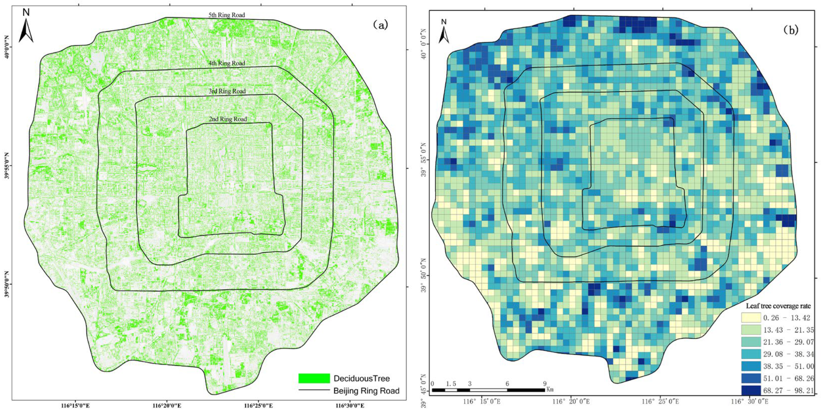
Figure 14a shows that the deciduous trees in the study area are evenly distributed in the inner/outer rings, with block-like clusters prominent in the fourth and fifth rings. Figure 14b (0.25 km2 grids) shows high-coverage grids mostly in the fourth and fifth rings (especially north/south, overlapping parks). Deciduous coverage ranges from 0.26–98.21% (avg 27.41%), with 42.81% of grids above average—nearly half the Fifth Ring Road area has coverage > 27.41%.
High-coverage deciduous tree clusters focus on the northern fourth to fifth rings, with fewer in the south. Though the fourth to fifth rings have the highest overall coverage, their southwest and southeast coverage is lower than the second ring—showing uneven north-high, south-low distribution here. The graph also shows that the second ring has the lowest deciduous coverage, which gradually increases from the second to fifth rings.
(4) Shrubs
According to Table 3, the total area covered by shrubs in the study area is 12.26 km2. The area within the fourth and fifth rings has the highest proportion, reaching 7.96 km2, accounting for 64.93%. The Second Ring Road has the lowest shrub coverage area, only 0.54 km2, accounting for 4.42%. The shrub coverage area between each ring is as follows: fourth to fifth rings (7.96 km2) > third to fourth rings (2.39 km2) > second to third rings (1.37 km2) > second ring (0.54 km2), showing a gradual increasing trend from the inner ring to the outer ring.
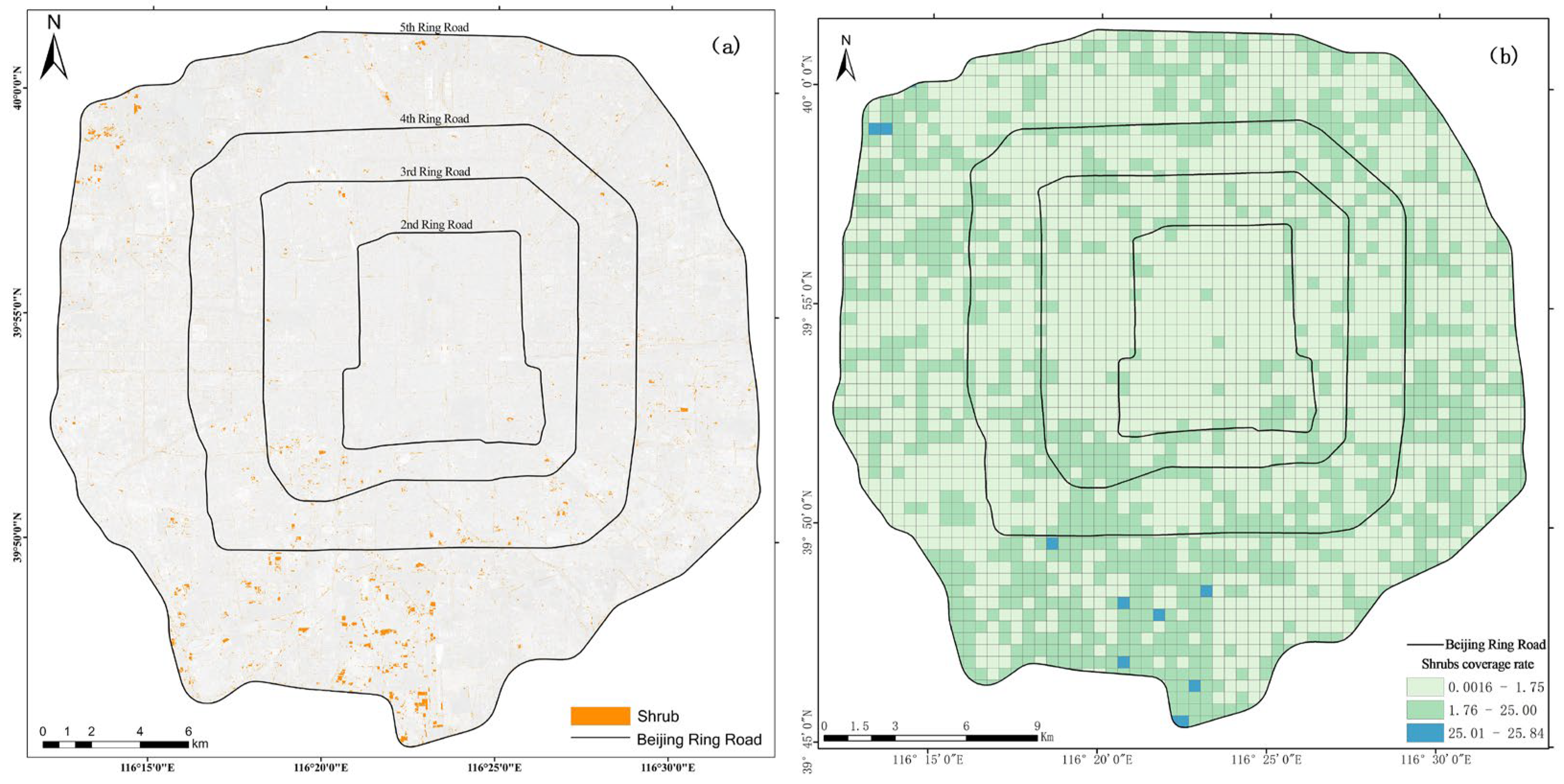
Figure 15a shows sparse shrub coverage in the study area. Figure 15b (0.25 km2 grids) shows high-shrub grids are partly in the fourth to fifth rings (mostly northwest/southeast) and partly align with Beijing’s ring roads (lane-oriented, overlapping ring road structure); they are also mostly axially distributed. Among all grids, shrub coverage ranges from 0.0016–25.84% (avg 2.12%), with 28.73% of grids above average—about a quarter of the area has coverage > 2.12%, with the rest mostly 0.0016–2.12%.
Within the fourth to fifth rings, shrub coverage tends to be clustered in parks. Between the second and fourth rings, the grids with high shrub coverage were mostly point-like and axial, and, in the axial distribution path, the grids with high shrub coverage showed a lower degree of aggregation.
(5) Grasslands
According to Table 3, the grassland coverage area in the study area is 29.88 km2, among which the grassland coverage area between the fourth and fifth rings is the highest, reaching 21.29 km2, accounting for 79.31%. The Second Ring Road has the lowest grassland coverage, only 0.64 km2, which accounted for 2.37%. The grassland coverage between each ring is as follows: fourth to fifth rings (21.29 km2) > third to fourth rings (3.50 km2) > second to third rings (1.45 km2) > second ring (0.64 km2), showing a gradual increasing trend from the inner ring to the outer ring.
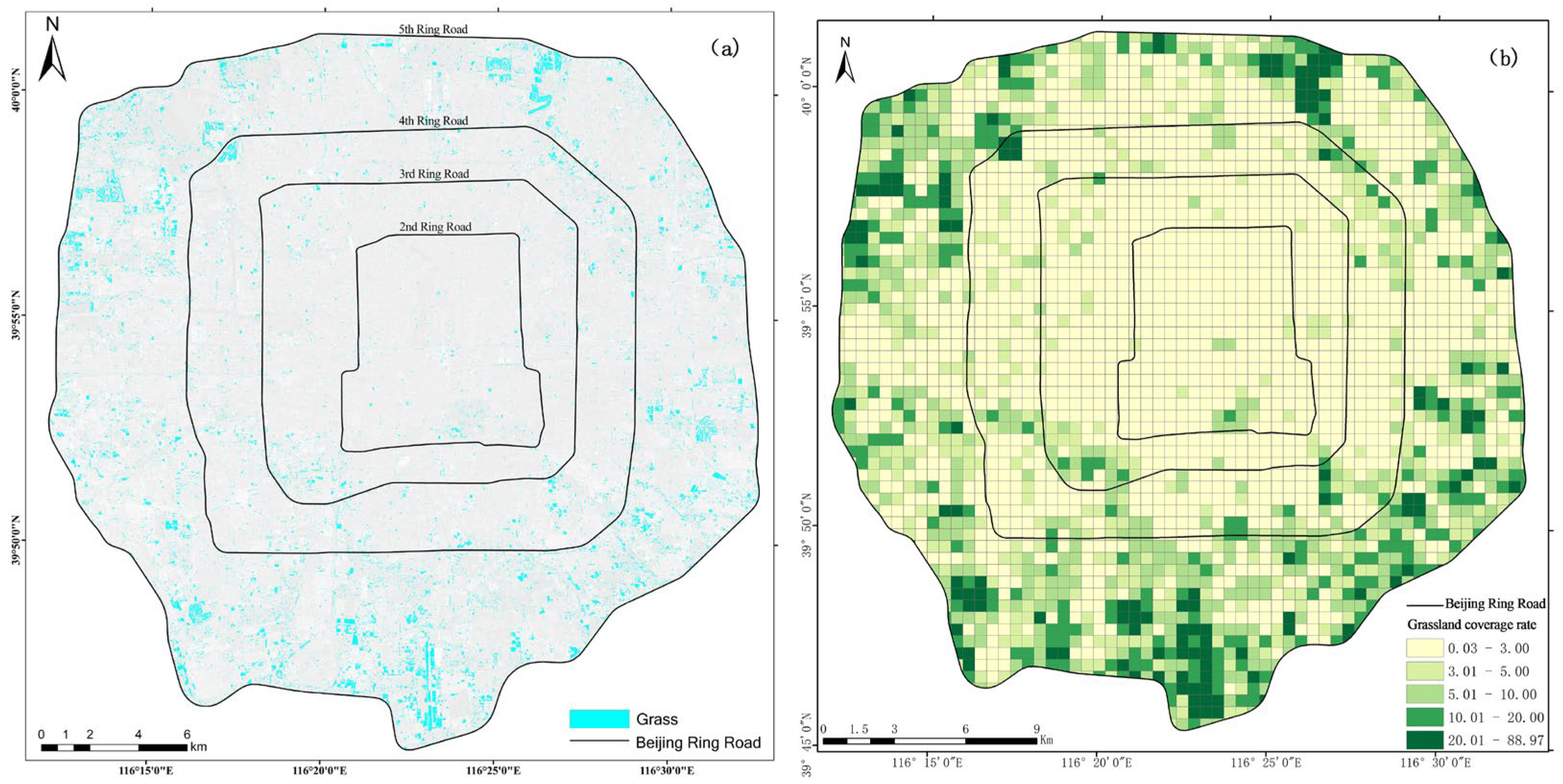
Figure 16a shows notable grassland coverage differences between rings, with most grasslands in distinct patches in the fourth to fifth rings. Figure 16b shows high-coverage grids mainly in the fourth to fifth rings’ northwest, northeast and southern areas; coverage is generally low in the second to fourth rings. Among all grids, grassland coverage ranges from 0.03–89.97% (avg 5.21%), with 28.55% of grids above average—a quarter of the area has coverage > 5.21% (mostly fourth to fifth rings), three-quarters 0.03–5.00% (mostly second–fourth rings). Darker grids mean higher coverage; grasslands in the fourth to fifth rings are mostly concentrated in parks.

4. Discussion

4.1. Precision Analysis of Deep Learning Models

Urban green space systems exhibit discrete spatial distribution and strong heterogeneity. When extracting information using remote sensing technology, they are easily disturbed by surrounding objects, resulting in reduced classification accuracy. This study conducted urban green space information extraction based on the YOLO v8 deep learning model. The results showed that this method has significant advantages in handling such complex scenarios. This finding is consistent with recent studies. For example, in vegetation species classification, deep learning achieved an overall accuracy of 94%, significantly better than SVM’s 91% [31], confirming the effectiveness of deep learning technology for the remote sensing monitoring of urban green spaces [32,33]. In addition, deep learning models have a stronger ability to fuse multi-source information [34] and can adaptively learn the most discriminative feature combinations even in cases of simple data distributions [35].
The purpose of this cross-task comparison is to analyze technical applicability, not model performance. Deep learning models can extract discriminative information beyond the spectrum, such as texture details and canopy structure, allowing them to distinguish evergreen and deciduous tree species and accurately separate shrubs from the background. In contrast, the MLC model, which relies solely on simple probability distribution assumptions, is prone to confusion when there is spectral overlap between different categories—for example, shrubs and grasslands may have similar NDVI values [36]. In this study, a large number of misclassifications of shrubs occurred with the MLC model, with user accuracy of only 47.95%. It can be seen that the spectral features extracted by pre-trained deep networks are more effective for distinguishing urban vegetation types than methods based solely on spectral overlap.
The SVM method can alleviate the problem of linear inseparability to some extent through kernel functions. However, in complex urban scenes with highly variable spectral classes and backgrounds, it tends to perform poorly, because it cannot fully utilize the spatial neighborhood information of pixels [26,37]. In this study, the misclassification rate of SVM was higher than that of MLC in the extraction of evergreen trees. This may be due to the large variety of evergreen tree species and diverse growth conditions in urban environments, which lead to greater spectral heterogeneity, and, consequently, unstable SVM decision boundaries [38,39].

4.2. Factors Affecting the Accuracy of Deep Learning Models

The strong classification performance of the YOLO v8 deep learning model largely depends on high-quality training data and appropriate training strategies. In this study, the data augmentation technique of flipped amplification was employed to effectively enhance the generalization ability and classification performance of the model. Data augmentation has a significant impact on improving the accuracy of deep learning models. Techniques such as random translation, rotation, and geometric transformations can significantly enrich the perspective variability of training samples and enhance the model’s robustness to changes in target morphology and background variations [40,41]. Especially in object detection for small targets, further data expansion through mirror flipping and rotation significantly improved the model’s recognition accuracy for small targets [42,43].
In this study, the training set was expanded four times through data augmentation based on the original annotations. The training curve of the model shows that the loss converges rapidly without overfitting, and the overall accuracy increases by 102.89%. This indicates that data augmentation significantly alleviates the problem of insufficient samples and enhances the generalization ability of the model. For vegetation-specific targets, Nie et al. [44] proposed data augmentation in the color space—such as adjusting the green tones of plants to simulate different seasons or health conditions—which improved the model’s ability to generalize across diverse appearances of green vegetation. The deep learning model improved accuracy by 13.4% compared to the un-data-enhanced DeepLabv3+ model. This indicates that sufficient and target-specific data augmentation has a significant impact on final classification accuracy when training deep learning models. In practical applications, the appropriate augmentation method should be selected according to the target features in order to achieve the optimal model performance.

4.3. Classification Differences Between Deep Learning Models and Traditional Models

The YOLO v8 deep learning model still has the problem of missing some small objects compared to traditional models. In this study, the model missed some shrubs and grasslands, possibly because these objects are small and scattered in remote sensing images and are easily ignored in information extraction. Khalili and Smyth proposed the SOD-YOLO v8 model by introducing a finer feature layer and improving the loss function, which increased the recall rate of YOLO v8 for small targets from 40.1% to 43.9%, significantly surpassing the original model [8]. This suggests that the base model of YOLO v8 may require further enhancements or integration with post-processing techniques when dealing with high-density small vegetation targets such as shrubs or grasslands in order to reduce the missed detection rate. In contrast, traditional pixel-level classification, with its pixel-by-pixel judgment, does not miss regions (each pixel is assigned a category), and, although it can fully label clustered small targets, it is prone to misclassification and has more noise [45,46,47]. In this study, MLC achieved a producer accuracy of 72.92% for grasslands—higher than the 56.38% achieved by SVM—indicating better identification of fragmented grassland areas. However, its user accuracy was only 50.84%, suggesting a high level of misidentification. Therefore, in order to further reduce the missed detection rate of target information, deep learning models can combine pixel detection preprocessing to optimize the effect.
Although deep learning models perform well, they are highly dependent on large-scale labeled datasets [48]. The YOLO v8 model exhibits three typical error categories in practical applications: (1) Inadequate feature learning for small targets, evidenced by significantly lower recall rates for 10 × 10 pixel-sized objects compared to medium and large targets; (2) deep network feature degradation, where the spatial information of small targets diminishes progressively as feature maps advance in depth; and (3) insufficient adaptability to complex scenarios, resulting in performance degradation under shadow occlusion and low-light conditions [46,47]. This study manually labeled nearly 80,000 greenfield instance elements to train the YOLO v8 deep learning model. In contrast, traditional machine learning models such as SVM and MLC can operate simply by selecting a limited number of regions of interest (ROI) pixels from the images, and the entire process is relatively fast. These traditional methods still have practical value when data are extremely limited or there is no sufficient computing power [49]. However, the development of transfer learning techniques is gradually alleviating this limitation. Deep models can be fine-tuned on smaller datasets using pre-trained weights, thereby reducing annotation requirements [50]. For example, Chen et al. [4] pre-trained U-net++ models on open datasets and then fine-tuned them for local urban vegetation classification. Their results showed that transfer learning could improve overall model accuracy by approximately 5%.
With the application of various improvement strategies, many of the limitations of deep learning models are being overcome. Single-stage detectors such as the YOLO series have become the preferred choice for remote sensing image target recognition by eliminating the candidate region generation step [51]. In land cover classification studies, the YOLO series has achieved accuracy levels several percentage points higher than traditional methods [52]. It is evident that deep learning models will play an increasingly important role in urban green space monitoring.

5. Conclusions

In this study, an urban green space classification model was constructed using the YOLO v8 deep learning algorithm, enabling the extraction and classification of green space information within complex urban environments. The results showed that the YOLO v8 deep learning model outperforms traditional methods in classifying all green space vegetation categories. Especially for tree and shrub targets, YOLO v8 significantly reduced misclassification and missed detections. Compared with the results obtained using SVM and MLC, the YOLO v8 model achieved an overall classification accuracy of 89.60% (Kappa = 0.798), which is significantly higher than the values of 71.53% (Kappa = 0.523) of SVM and 69.57% (Kappa = 0.551) of MLE. Among the classification results of the YOLO v8 deep learning model, the user accuracy for evergreen trees, deciduous trees, and grasslands was all above 90%, and that of shrubs was 88.9%. The producer accuracy for each type was above 85%. This indicates that YOLO v8 has good compatibility and high accuracy in northern temperate cities, with Beijing as a typical example.
The coverage of different types of green spaces within Beijing’s Fifth Ring Road increases from the central urban area to the periphery. High-coverage areas are mainly concentrated in parks and green spaces within the Fourth and Fifth Ring Roads, with varying degrees of vegetation clustering. Specifically, evergreen trees are concentrated around the periphery, with low and uniform coverage in the central area; high coverage zones are found in parks in the northwest and southeast of the fourth and fifth rings. Deciduous trees are clustered in blocks around the fourth and fifth rings, particularly in the north. Shrub green spaces are distributed along the main roads and along the axis of the ring roads. There is a certain concentration in the parks around the fourth and fifth rings, though overall coverage is low and scattered. Grassland green spaces are distributed in blocks and are more concentrated in the northwest, northeast and south of the fourth and fifth rings.
In the process of extracting for different green space types, the shading of shrubs and grasslands by evergreen and deciduous trees in the green space categories was not taken into account, resulting in the possible underestimation of shrub and grassland areas. To address occlusion errors, the model incorporates an attention mechanism by integrating a Convolutional Block Attention Module (CBAM) into its backbone network. This enhancement strengthens feature responses in unobstructed regions while suppressing interference from occluded areas. Furthermore, the model employs a Squeeze-and-Excitation (SE) module to enable the adaptive selection of feature channels, allowing it to prioritize features from unobstructed regions or utilize multimodal data (e.g., infrared + visible light) for supplementary recognition. Future studies should consider adding laser height measurement data to eliminate the shading effect of tall trees on low shrubs and grass in order to further improve the classification performance of the model. Vegetation classification technology provides objective quantitative data for policy making by accurately identifying urban vegetation types, distribution, and coverage, addressing issues of “information ambiguity” and “weak targeting”. First, it differentiates green space categories to clarify supply variations between old and new urban areas, supporting decisions such as demolition for greening and pocket park construction. Second, it distinguishes multi-layered vegetation from single-layer lawns, leveraging data showing “20% reduction in residents’ psychological stress in multi-layered vegetation zones” to support policies for “urban forests” and “healing gardens” that enhance public health. Third, it evaluates vegetation area and growth status to accurately estimate regional biomass, providing support for carbon sink policies.

Author Contributions

Conceptualization, B.L. and X.X.; data curation, B.L. and X.X.; writing—original draft preparation, Y.D. and H.W.; writing—review and editing, B.L., X.X., N.Z., S.L. (Shaoning Li) and S.L. (Shaowei Lu); supervision, B.L.; project administration, X.X., X.L., Y.S. and S.L. (Shaoning Li); funding acquisition, B.L., X.X. and S.L. (Shaowei Lu). All authors have read and agreed to the published version of the manuscript.

Funding

This research was funded by the Director’s Foundation of Institute of Forestry and Pomology in Beijing Academy of Agriculture and Forestry Sciences (Grant No. LGSSZJJ202302).

Data Availability Statement

The original contributions presented in the study are included in the article, and further inquiries can be directed to the corresponding author.

Acknowledgments

Thanks to the following units for supporting this research: the Institute of Forestry and Pomology, Beijing of Agriculture and Forestry Sciences; Beijing Yanshan Forest Ecosystem Observation and Research Station; and the Forestry College of Shenyang Agricultural University.

Conflicts of Interest

The authors declare no conflicts of interest.

References

  1. Ahmed, F.; Noor, W.; Nasim, M.A.; Ullah, I.; Basit, A. Vegetation and Non-Vegetation Classification Using Object Detection Techniques and Deep Learning from Low/Mixed Resolution Satellite Images. Pak. J. Emerg. Sci. Technol. 2023, 4, 1–18. [Google Scholar]
  2. Burrewar, S.S.; Haque, M.; Haider, T.U. A Survey on Mapping of Urban Green Spaces within Remote Sensing Data Using Machine Learning & Deep Learning Techniques. In Proceedings of the 15th International Conference on Computer and Automation Engineering, Sydney, NSW, Australia,, 3–5 March 2023; Institute of Electrical and Electronics Engineers: Piscataway, NJ, USA, 2023. [Google Scholar]
  3. Chan, R.H.; Kan, K.K.; Nikolova, M.; Plemmons, R.J. A two-stage method for spectral–spatial classification of hyperspectral images. J. Math. Imaging Vis. 2020, 62, 790–807. [Google Scholar]
  4. Chen, S.; Zhang, M.; Lei, F. Mapping Vegetation Types by Different Fully Convolutional Neural Network Structures with Inadequate Training Labels in Complex Landscape Urban Areas. Forests 2023, 14, 1788. [Google Scholar] [CrossRef]
  5. Chen, Y.; Weng, Q.; Tang, L.; Liu, Q.; Zhang, X.; Bila, M. Automatic mapping of urban green spaces using a geospatial neural network. GIScience Remote Sens. 2021, 58, 624–642. [Google Scholar]
  6. Deng, C.; Wu, C. BCI: A biophysical composition index for remote sensing of urban environments. Remote Sens. Environ. 2012, 127, 247–259. [Google Scholar]
  7. Xu, S.; Wang, R.; Shi, W.; Wang, X. Classification of Tree Species in Transmission Line Corridors Based on YOLO v7. Forests 2024, 15, 61. [Google Scholar] [CrossRef]
  8. Khalili, B.; Smyth, A.W. SOD-YOLOv8—Enhancing YOLOv8 for Small Object Detection in Aerial Imagery and Traffic Scenes. Sensors 2024, 24, 6209. [Google Scholar] [CrossRef]
  9. Foody, G.M. Status of land cover classification accuracy assessment. Remote Sens. Environ. 2002, 80, 185–201. [Google Scholar]
  10. Noi, P.T.; Kappas, M. Comparison of Random Forest, k-Nearest Neighbor, and Support Vector Machine Classifiers for Land Cover Classification Using Sentinel-2 Imagery. Sensors 2018, 18, 18. [Google Scholar]
  11. Franchi, G.; Angulo, J.; Sejdinovic, D. Hyperspectral image classification with support vector machines on kernel distribution embeddings. In Proceedings of the 2016 IEEE International Conference on Image Processing (ICIP), Phoenix, AZ, USA, 25–28 September 2016; pp. 1898–1902. [Google Scholar]
  12. Hao, X.; Liu, L.; Yang, R.; Yin, L.; Zhang, L.; Li, X. A Review of Data Augmentation Methods of Remote Sensing Image Target Recognition. Remote Sens. 2023, 15, 827. [Google Scholar]
  13. Hasan, M.; Ullah, S.; Khan, M.J.; Khurshid, K. Comparative Analysis of SVM, ANN and CNN for Classifying Vegetation Specie using Hyperspectral Thermal Infrared Data. Int. Arch. Photogramm. Remote Sens. Spat. Inf. Sci. 2019, XLII-2/W13, 1861–1868. [Google Scholar] [CrossRef]
  14. Javed, A.; Cheng, Q.; Peng, H.; Altan, O.; Li, Y.; Ara, I.; Huq, E.; Ali, Y.; Saleem, N. Review of Spectral Indices for Urban Remote Sensing. Photogramm. Eng. Remote Sens. 2021, 87, 513–524. [Google Scholar] [CrossRef]
  15. Kadhim, I.; Abed, F.M.; Vilbig, J.M.; Sagan, V.; DeSilvey, C. Combining Remote Sensing Approaches for Detecting Marks of Archaeological and Demolished Constructions in Cahokia’s Grand Plaza, Southwestern Illinois. Remote Sens. 2023, 15, 1057. [Google Scholar] [CrossRef]
  16. Na, L.; Jing, H.; Bin, W.; Feifei, T.; Junyu, Z.; Jiang, G. Intelligent Extraction of Urban Vegetation Information based on Vegetation Spectral Signature and Sep-U Net. J. Geo-Inf. Sci. 2023, 25, 1717–1729. [Google Scholar]
  17. Liu, W.; Yue, A.; Shi, W.; Ji, J.; Deng, R. An Automatic Extraction Architecture of Urban Green Space Based on DeepLabv3plus Semantic Segmentation Model. In Proceedings of the IEEE 4th International Conference on Image, Vision and Computing, Xiamen, China, 5–7 July 2019; Institute of Electrical and Electronics Engineers: Piscataway, NJ, USA, 2019. [Google Scholar]
  18. Liu, Y.; Zhong, Y.; Shi, S.; Zhang, L. Scale-aware deep reinforcement learning for high resolution remote sensing imagery classification. ISPRS J. Photogramm. Remote Sens. 2024, 209, 296–311. [Google Scholar] [CrossRef]
  19. Li, B.; Xu, X.; Wang, H.; Duan, Y.; Lei, H.; Liu, C.; Zhao, N.; Liu, X.; Li, S.; Lu, S. Analysis and Comprehensive Evaluation of Urban Green Space Information Based on Gaofen 7: Considering Beijing’s Fifth ring Area as an Example. Remote Sens. 2024, 16, 3946. [Google Scholar] [CrossRef]
  20. Li, Y.; Li, Q.; Pan, J.; Zhou, Y.; Zhu, H.; Wei, H.; Liu, C. SOD-YOLO: Small-Object-Detection Algorithm Based on Improved YOLO v8 for UAV Images. Remote Sens. 2024, 16, 3057. [Google Scholar] [CrossRef]
  21. Nawaz, S.A.; Li, J.; Bhatti, U.A.; Shoukat, M.U.; Ahmad, R.M. AI-based object detection latest trends in remote sensing, multimedia and agriculture applications. Front. Plant Sci. 2022, 13, 1041514. [Google Scholar] [CrossRef]
  22. Ramos, L.T.; Sappa, A.D. Leveraging U-Net and selective feature extraction for land cover classification using remote sensing imagery. Sci. Rep. 2025, 15, 784. [Google Scholar] [CrossRef]
  23. Rochefort-Beaudoin, T.; Vadean, A.; Achiche, S.; Aage, N. From density to geometry: Instance segmentation for reverse engineering of optimized structures. Eng. Appl. Artif. Intell. 2025, 141, 109732. [Google Scholar] [CrossRef]
  24. Ruiz-Ponce, P.; Ortiz-Perez, D.; Garcia-Rodriguez, J.; Kiefer, B. POSEIDON: A Data Augmentation Tool for Small Object Detection Datasets in Maritime Environments. Sensors 2023, 23, 3691. [Google Scholar] [CrossRef]
  25. Sekertekin, A.; Marangoz, A.M.; Akcin, H. Pixel-based Classification Analysis of Land Use Land Cover Using Sentiel-2 and Landsat-8 Data. Int. Arch. Photogramm. Remote Sens. Spat. Inf. Sci. 2017, XLII, 91–93. [Google Scholar] [CrossRef]
  26. Zhang, M.; Arshad, H.; Abbas, M.; Jehanzeb, H.; Tahir, I.; Hassan, J.; Samad, Z.; Chunara, R. Quantifying Greenspace with Satellite Images in Karachi, Pakistan, Using a New Data Augmentation Paradigm. ACM J. Comput. Sustain. Soc. 2025, 3, 1–23. [Google Scholar] [CrossRef]
  27. Cheng, Y.; Wang, W.; Ren, Z.; Zhao, Y.; Liao, Y.; Ge, Y.; Wang, J.; He, J.; Gu, Y.; Wang, Y.; et al. Multi-scale feature fusion and transformer network for urban green space segmentation from high-resolution remote sensing images. Int. J. Appl. Earth Obs. Geoinf. 2024, 132, 103586. [Google Scholar] [CrossRef]
  28. Xu, W.; Zhang, H.; Zhang, Y.; Liu, K.; Zhang, J.; Zhu, Y.; Dilixiati, B.; Ning, J.; Gao, J. YOLO-DS: A detection model for desert shrub identification and coverage estimation in UAV remote sensing. J. For. Res. 2025, 36, 116. [Google Scholar] [CrossRef]
  29. Shi, D.; Yang, X. Support Vector Machines for Land Cover Mapping from Remote Sensor Imagery. In Monitoring and Modeling of Global Changes: A Geomatics Perspective; Springer: Berlin/Heidelberg, Germany, 2015; pp. 265–279. [Google Scholar]
  30. Shi, Q.; Liu, M.; Marinoni, A.; Liu, X. UGS-1m: Fine-grained urban green space mapping of 31 major cities in China based on the deep learning framework. Earth Syst. Sci. Data 2023, 15, 555–577. [Google Scholar] [CrossRef]
  31. Tran, T.V.; Julian, J.P.; De Beurs, K.M. Land Cover Heterogeneity Effects on Sub-Pixel and Per-Pixel Classifications. ISPRS Int. J. Geo-Inf. 2014, 3, 540–553. [Google Scholar] [CrossRef]
  32. Wang, Y.; Duan, H. Classification of Hyperspectral Images by SVM Using a Composite Kernel by Employing Spectral, Spatial and Hierarchical Structure Information. Remote Sens. 2018, 10, 441. [Google Scholar] [CrossRef]
  33. Wu, T.; Dong, Y. YOLO-SE: Improved YOLO v8 for Remote Sensing Object Detection and Recognition. Appl. Sci. 2023, 13, 12977. [Google Scholar] [CrossRef]
  34. Xu, C.; Gao, L.; Su, H.; Zhang, J.; Wu, J.; Yan, W. Label Smoothing Auxiliary Classifier Generative Adversarial Network with Triplet Loss for SAR Ship Classification. Remote Sens. 2023, 15, 4058. [Google Scholar] [CrossRef]
  35. Yan, Y.; Tan, Z.; Su, N. A Data Augmentation Strategy Based on Simulated Samples for Ship Detection in RGB Remote Sensing Images. ISPRS Int. J. Geo-Inf. 2019, 8, 276. [Google Scholar] [CrossRef]
  36. Yan, Y.; Zhang, Y.; Su, N. A Novel Data Augmentation Method for Detection of Specific Aircraft in Remote Sensing RGB Images. IEEE Access 2019, 7, 56051–56061. [Google Scholar] [CrossRef]
  37. Yao, Z.Y.; Liu, J.J.; Zhao, X.W.; Long, D.F.; Wang, L. Spatial dynamics of above ground carbon stock in urban green space: A case study of Xi’an, China. J. Arid Land 2015, 7, 350–360. [Google Scholar] [CrossRef]
  38. Du, X.; Wang, G.; Lu, C.; Yan, Z.; Zhang, T. Green space extraction from Resource-3 remote sensing images in complex urban environments. J. Remote Sens. 2024, 28, 2954–2969. [Google Scholar]
  39. Hu, X.; Lou, L.; Zhou, X. Design and implementation of Urban Remote Sensing Image Processing System Based on Deep learning. Mod. Comput. 2023, 29, 25–29. [Google Scholar]
  40. Huang, F.; Cao, F.; Wang, Q. Research on Fine Classification of Urban Green Spaces by fusing GF-2 and Open Map Data. Resour. Dev. Mark. 2024, 40, 321–329. [Google Scholar]
  41. Li, G.; Qiao, Y.; Wu, W.; Zheng, Y.; Hong, Y.; Zhou, X. Deep learning and its applications in computer vision. J. Comput. Appl. 2019, 36, 3521–3529+3564. [Google Scholar]
  42. Liu, W.; Yue, A.; Ji, J.; Shi, W.; Deng, R.; Liang, Y.; Xiong, L. GF-2 image urban green space extraction based on DeepLabv3+ Semantic segmentation Model. Remote Sens. Land. Resour. 2020, 32, 120–129. [Google Scholar]
  43. Men, G. Research on the Extraction Method and Spatio-Temporal Variation of Green Space Information from High-Resolution Images of the Pearl River Delta Urban Agglomeration. Master’s Thesis, University of Chinese Academy of Sciences, Beijing, China, 2022. [Google Scholar]
  44. Nie, Z. Research on Changes in Urban Green Spaces in China Based on Multi-source Remote Sensing data. Acta Geod. Sin. 2024, 53, 205. [Google Scholar]
  45. Yan, J.; Tang, S. Research on the application of unmanned Aerial Vehicle remote sensing in Urban landscaping survey. Jiangxi Commun. Sci. Technol. 2024, 1, 37–41. [Google Scholar]
  46. Ziyuan, Z.; Miao, C.; Lian, H. An improved small object and slender target detection model based on YOLOv8. Comput. Appl. 2024, 44, 286–295. [Google Scholar]
  47. Jian, W.; Di, X.; Lihang, F.; Cheng, S. A PCB Small Object Defect Detection Model Based on Improved YOLOv8s. Comput. Eng. Appl. 2025, 61, 288–297. [Google Scholar]
  48. Zhao, Y.; Zhang, N.; Xu, M. Comparison and Analysis of Remote Sensing Image Interpretation Methods for Geographic National Conditions Monitoring. Surv. Mapp. Spat. Geogr. Inf. 2021, 1, 103–105. [Google Scholar]
  49. Yang, Y.; Sun, W.; Su, G. A Novel Support-Vector-Machine-Based Grasshopper Optimization Algorithm for Structural Reliability Analysis. Buildings 2022, 12, 855. [Google Scholar] [CrossRef]
  50. Gong, F.; Zheng, Z.C.; Ng, E. Modeling Elderly Accessibility to Urban Green Space in High Density Cities: A Case Study of Hong Kong. Procedia Environ. Sci. 2016, 36, 90–97. [Google Scholar] [CrossRef]
  51. Habibollah, F.; Taher, P. Analysis of spatial equity and access to urban parks in Ilam, Iran. J. Environ. Manag. 2020, 260, 110–122. [Google Scholar] [CrossRef]
  52. Huang, Y.Y.; Lin, T.; Zhang, G.Q. Spatiotemporal patterns and inequity of urban green space accessibility and its relationship with urban spatial expansion in China during rapid urbanization period. Sci. Total Environ. 2021, 809, 151123. [Google Scholar] [CrossRef] [PubMed]
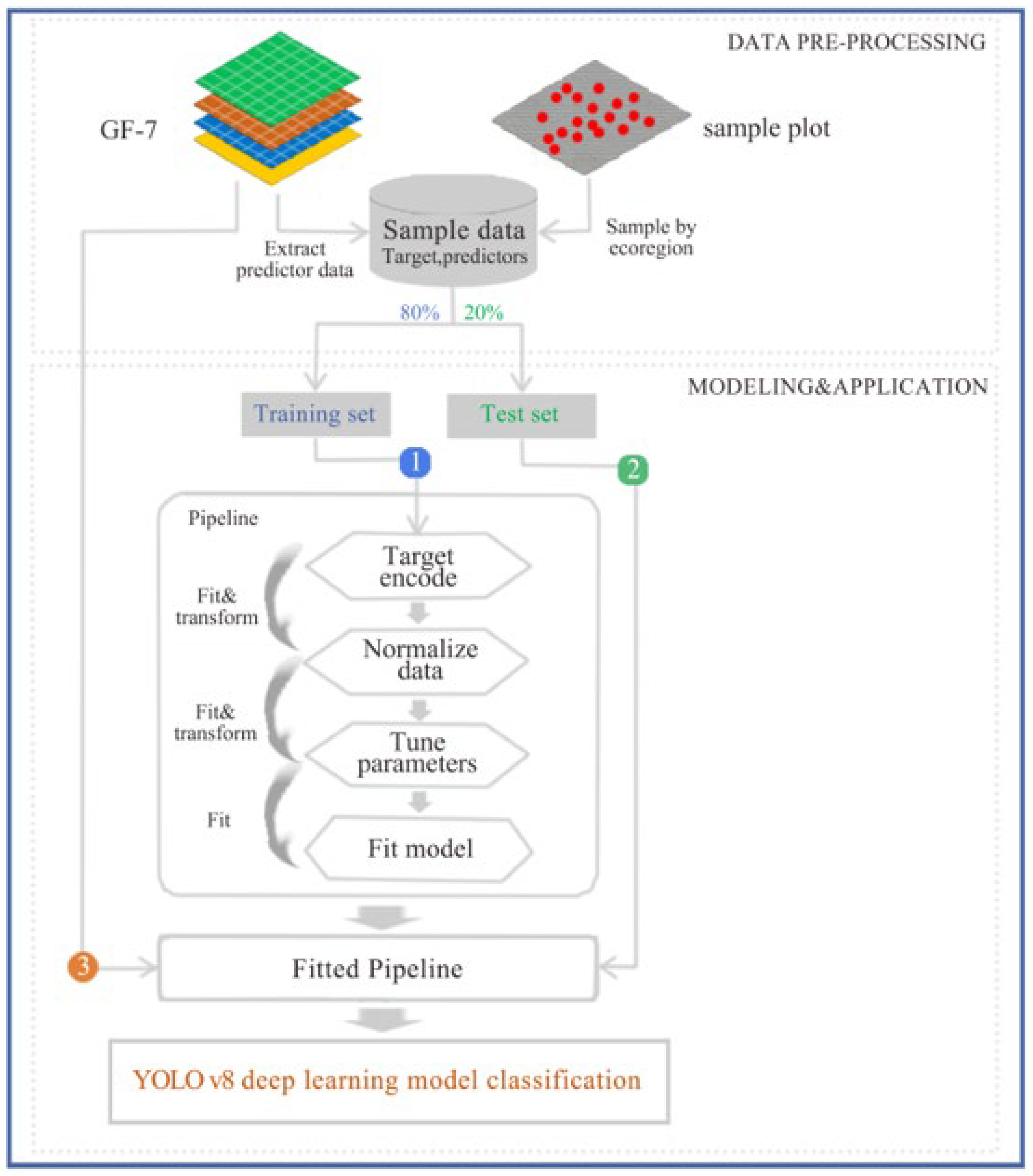
Figure 1. Flowchart of the method.
Land 14 02005 g001
Figure 2. Distribution of sample labels.
Land 14 02005 g002
Figure 3. Sample label data enhancement diagram.
Land 14 02005 g003
Figure 4. Number of vegetation elements in the sample set by type.
Land 14 02005 g004
Figure 5. Training accuracy and loss curve of the YOLO v8 deep learning model. (a) the classification accuracy of the model; (b) the loss value of the training.
Land 14 02005 g005
Figure 6. User accuracy confusion matrix of three algorithms.
Land 14 02005 g006
Figure 7. Three algorithms produce precision confusion matrices.
Land 14 02005 g007
Figure 8. Comparison of evergreen tree classification results of three different algorithms in the sample area. (a) the evergreen tree label image (green = true values); (bd) yellow denotes correct predictions of YOLO v8, SVM, and MLC sequentially; (eh) red represents misclassifications.
Land 14 02005 g008
Figure 9. Comparison of deciduous tree classification performance using three different algorithms in the sample area. (a) the deciduous tree label image (green = true values); (bd) yellow denotes correct predictions of YOLO v8, SVM, and MLC sequentially; (eh) red represents misclassifications.
Land 14 02005 g009
Figure 10. Comparison of shrub classification performance using three different algorithms in the sample area. (a) the sample area’s shrub label image (green = true values); (bd) yellow denotes correct predictions of YOLO v8, SVM, and MLC sequentially; (eh) red represents misclassifications.
Land 14 02005 g010
Figure 11. Comparison of grassland classification performance among three different algorithms in the sample area. (a) the sample area’s grassland label image (green = true values); (bd) yellow denotes correct predictions of YOLO v8, SVM, and MLC sequentially; (eh) red represents misclassifications.
Land 14 02005 g011
Figure 12. Classification results of green spaces in the Fifth Ring Road of Beijing.
Land 14 02005 g012
Figure 13. Distribution map of evergreen trees and their coverage in the Fifth Ring Road of Beijing. (a) the overall distribution of evergreen tree green space vegetation in the study area; (b) high evergreen tree coverage.
Land 14 02005 g013
Figure 14. (a) Distribution map of deciduous trees; and (b) spatial distribution of deciduous tree coverage within the Fifth Ring Road of Beijing.
Land 14 02005 g014
Figure 15. (a) Distribution map of shrubs; and (b) shrub coverage distribution map within the Fifth Ring Road of Beijing.
Land 14 02005 g015
Figure 16. (a) Distribution map of grassland; and (b) grassland coverage distribution within the Fifth Ring Road of Beijing.
Land 14 02005 g016
Table 1. Accuracy evaluation metrics for green space classification models.
Green Space Classification Accuracy Evaluation IndexCalculation Formula
OA O A = n i = 1 C i i n i = 1 n j = 1 C i j
Kappa K = N n i = 1 X i i n i = 1 X i + × X + i N 2 n i = 1 X i + × X + i
UA U A i = C i i n i = 1 C i j
PA P A i = C i i n j = 1 C j i
F1 score F 1 i = 2 C i i n j = 1 C i j + n i = 1 C j i
Note: represents the diagonal elements of the confusion matrix, indicating the number of instances where the true class and predicted class are both i; is the sum of the i-th row in the confusion matrix, representing the total number of predictions for class i; is the sum of the i-th column in the confusion matrix, representing the total number of instances predicted as class i, where is the number of classes; is the sum of instances in the i-th row, and is the sum of instances in the i-th column; is the diagonal element of the matrix; and is the total number of different classes.
Table 2. Comparison of classification accuracy across three methods.
Classification ModelOverall Classification Accuracy (%)Kappa CoefficientF1 Score
YOLO v889.600.7980.860
SVM71.530.5230.715
MLC69.570.5510.696
YOLO v8 (no augmentation)42.190.0920.422
Table 3. Classification accuracy of green vegetation types by different algorithms.
YOLO v8SVMMLC
Evergreen trees92.67%46.27%61.14%
Deciduous trees95.69%63.30%40.73%
Shrubs89.08%25.27%47.88%
Grassland89.06%46.74%55.82%
Table 4. Different types of green space area of research area.
Research AreaEvergreen Trees
(km2)
Deciduous Trees (km2)Shrubs (km2)Grasslands (km2)
Within the
Second Ring Road
0.8912.420.540.64
Within the second–third rings0.3420.461.371.45
Within the third–fourth rings0.7430.022.393.50
Within the fourth–fifth rings4.2680.087.9621.29
Total (within five rings)6.23142.9712.2626.88
Disclaimer/Publisher’s Note: The statements, opinions and data contained in all publications are solely those of the individual author(s) and contributor(s) and not of MDPI and/or the editor(s). MDPI and/or the editor(s) disclaim responsibility for any injury to people or property resulting from any ideas, methods, instructions or products referred to in the content.