Accurate Identification of High-Potential Reserved Cultivated Land Resources: A Convolutional Neural Network-Based Intelligent Selection Framework Verified in Qinghai Province on the Qinghai–Tibet Plateau, China

Abstract

The sustainable use of farmland depends on the precise identification of promising reserved cultivated land resources, particularly in regions with fragmented spatial patterns and complex environmental conditions. Traditional evaluation methods often rely on limited indicators and neglect patch morphology, leading to restricted accuracy and applicability. To address this issue, an innovative intelligent-selection framework is proposed that integrates multi-source data evaluation with patch-morphology verification and employs convolutional neural networks (CNNs), applied in Qinghai Province, China. The framework combines one-dimensional and two-dimensional CNN models, incorporating 11 key indicators—including slope, irrigation conditions, and contiguity—together with patch morphology to predict development priority. Results show that the two models achieve predictive accuracies of 98.48% and 91.95%, respectively, outperforming the traditional Analytic Hierarchy Process (AHP) and effectively filtering out irregular patches unsuitable for cultivation. Further SHAP analysis and ablation experiments reveal the contributions of individual indicators, with slope identified as the dominant factor in prioritization. Overall, the study demonstrates that integrating multi-source data evaluation with patch-morphology verification within a machine-learning framework significantly enhances prioritization accuracy. The proposed framework provides a transferable, evidence-based pathway for the graded utilization of reserved cultivated land resources and the reinforcement of farmland security strategies.

1. Introduction

Arable land resources constitute the foundation of agricultural production and play a pivotal role in ensuring food security [1,2,3]. However, since the early 21st century, accelerated population growth and urbanization have led to a decline in the area of high-quality arable land and an imbalance in its spatial distribution [4,5], thereby threatening arable land security and severely limiting its multiple functions [6,7]. Society has become ever more aware of the importance of arable land protection, and how to achieve both conservation and optimized utilization of limited land resources has emerged as a critical challenge in the fields of land management and spatial planning [8,9].

Reserved cultivated land resources refer to potential farmland that can be converted into arable land under existing natural, economic, and technical conditions through measures such as land consolidation, irrigation improvement, or strategic allocation. In 1998, the central government of China introduced the arable land occupation–compensation balance policy, designating the development of reserved cultivated land resources as a key approach for supplementing arable land [1]. This approach has helped reconcile the tension between the reduction in arable land resources and the expansion of urban construction land, thereby ensuring a balanced regional arable land base [10]. However, with continued exploitation, both the quantity and quality of reserved cultivated land resources have declined, resulting in fragmented distributions and increasingly complex terrain. Consequently, high-precision evaluation methods are required to comprehensively analyze their cultivability. Hierarchical classification and suitability assessment of reserved cultivated land resources can provide a scientific basis for compensation and dynamic management [11]. Rational development and utilization of these resources can alleviate human–land conflicts, safeguard food supply, and, through optimized land-use patterns, offer effective pathways for sustainable agricultural development.

Existing evaluations of reserved cultivated land resources have explored various evaluation units, methods, and indicator systems from different perspectives [12,13,14]. Most studies use current land-use maps or grid cells as evaluation units, constructing indicator systems focused on natural conditions, ecological security, natural suitability, and economic feasibility, and selecting representative factors [15,16,17]. Commonly used methods include the analytic hierarchy process (AHP) [18,19,20,21], the analytic network process (ANP) [22], ordered weighted averaging (OWA) [23], logic scoring of preference [24], and fuzzy modeling [25,26,27]. Integration with 3S technologies (GIS, GPS, RS) has further enhanced the intuitiveness of both evaluation processes and results [10]. Among these, AHP is widely favored for its combination of qualitative and quantitative analysis, clear hierarchy, and ease of use; however, its reliance on expert judgment for weight determination limits objectivity [20]. To mitigate this, researchers have integrated AHP with fuzzy methods [28,29] and gray relational analysis [30] to improve weight allocation.

In recent years, machine-learning methods such as convolutional neural networks (CNN) [31,32,33], support vector machines [34], and random forests [34] have been widely applied in geospatial evaluations due to their ability to model complex nonlinear relationships and reduce subjective human intervention. The typical workflow for machine-learning-based evaluation includes data preparation and partitioning, model selection and construction, model training and optimization, and application of the trained model for evaluation. Although these methods excel at uncovering nonlinear relationships among input variables, their “black-box” nature prevents explicit mapping between input factors and evaluation outcomes [35]. Model accuracy is heavily influenced by the quantity and quality of training samples [36]. Beyond the algorithms themselves, input data characteristics—such as slope, soil physicochemical properties, climate, and accessibility—also significantly impact evaluation outcomes [37]. An increasing number of studies have attempted to incorporate explainable artificial intelligence methods to enhance the transparency and usability of prediction processes [38]. In recent years, SHAP has been widely applied to reveal factor contributions and interpret model performance, thereby alleviating the “black-box” issue [39,40]. Related research has also introduced deep-learning frameworks into soil resource management to optimize sampling strategies and ensure data representativeness [41], as well as demonstrated superior performance in predicting land suitability for staple crops [42]. Meanwhile, the combination of deep learning and UAVs has provided new perspectives for farmland quality assessment [43], and the integration of AI with explainable approaches has shown additional potential in crop yield prediction and agricultural decision-making [44]. Despite the diversity of factor selection and model design in existing reserved cultivated land evaluation, several limitations remain: (1) few studies incorporate geometric features such as patch shape and contiguity; (2) many depend on expert judgment or linear weight functions, introducing potential bias; and (3) traditional models struggle to support nonlinear coupling among multiple factors and cannot directly quantify development potential at fine spatial scales.

With the advancement of machine-learning techniques, new avenues have opened for selecting high-quality reserved cultivated land resources. CNN can automatically extract features from raw evaluation data of reserved cultivated land resources, capture complex nonlinear relationships, and simultaneously incorporate patch morphology; by training on high-quality samples, they learn more precise patterns and rules, thereby enhancing the accuracy of reserved cultivated land resources evaluation. However, applications of machine learning in reserved cultivated land evaluation remain limited, and few studies have addressed the entire Qinghai Province. To fill this gap, the present study integrates geographic information systems (GIS) and statistical datasets, employs machine-learning methods to develop a dual-screening model based on one-dimensional (1D-CNN) and two-dimensional convolutional neural networks (2D-CNN), and embeds patch morphology into the evaluation process. We propose an intelligent-selection framework that fuses multi-source data evaluation with morphological verification and validate its application in Qinghai Province. The primary objectives are: (1) to perform a priority-ranking evaluation of reserved cultivated land resources in Qinghai Province; (2) to verify the accuracy and efficiency of CNN models in reserved cultivated land resources evaluation; and (3) to explore the cross-domain potential of the proposed framework. The intelligent-selection framework presented herein is designed to support the efficient development and precise utilization of regional reserved cultivated land resources, thereby advancing their scientific planning and sustainable management at broader scales.

2. Materials and Methods

2.1. Study Area

Qinghai Province is located in western China, on the northeastern edge of the Tibetan Plateau, with its capital in Xining City (Figure 1). Its geographic coordinates extend from 89°24′3″ E to 103°04′10″ E and from 31°36′2″ N to 39°12′45″ N, spanning approximately 1241 km east–west and 845 km north–south. Covering about one-thirteenth of China’s total land area, Qinghai is the fourth largest province-level region, after Xinjiang Uygur, Xizang, and Inner Mongolia autonomous regions. It borders Gansu Province to the northeast, Sichuan Province to the southeast, Xinjiang Uygur Autonomous Region to the northwest, and Xizang Autonomous Region to the southwest. Qinghai has a highland continental climate characterized by low temperatures, large diurnal temperature variations, scarce but concentrated precipitation, long sunshine duration, and strong solar radiation. Winters are long and severe, while summers are short and cool, with marked regional climatic differences. Reserved cultivated land resources in Qinghai are highly fragmented and limited in overall area, making the province an ideal case study for validating the proposed framework.

2.2. Data Sources

The datasets used in this study include (1) DEM data (90 m resolution, 2025) obtained from the NASA Earthdata portal (https://earthdata.nasa.gov/), accessed on 12 September 2024, which were used to derive elevation and slope. (2) Effective soil-layer thickness (1 km resolution, 2018), soil texture (1 km resolution, 2018), soil pH (1 km resolution, 2018), and soil organic-matter content (1 km resolution, 2018), obtained from survey results published by local government agencies in Qinghai Province. Although the “Third National Land Resource Survey” in China has been largely completed, the soil-specific results have not yet been fully compiled, publicly released, or made available in complete downloadable form. Consequently, this study relies on soil data from 2018, which may introduce uncertainties regarding the spatial resolution and practical representativeness of the evaluation. (3) Irrigation conditions, transportation accessibility, cultivation accessibility, and contiguity, calculated using geospatial analysis of 2023 land-use change data. (4) Air temperature (1 km resolution, 2024) and precipitation (1 km resolution, 2024), obtained from the National Earth System Science Data Center (https://www.geodata.cn/main/), accessed on 12 September 2024. (5) Reserved cultivated land resources inventory, provided by the Land Consolidation and Ecological Restoration Center, Qinghai Province, China.

2.3. Methods

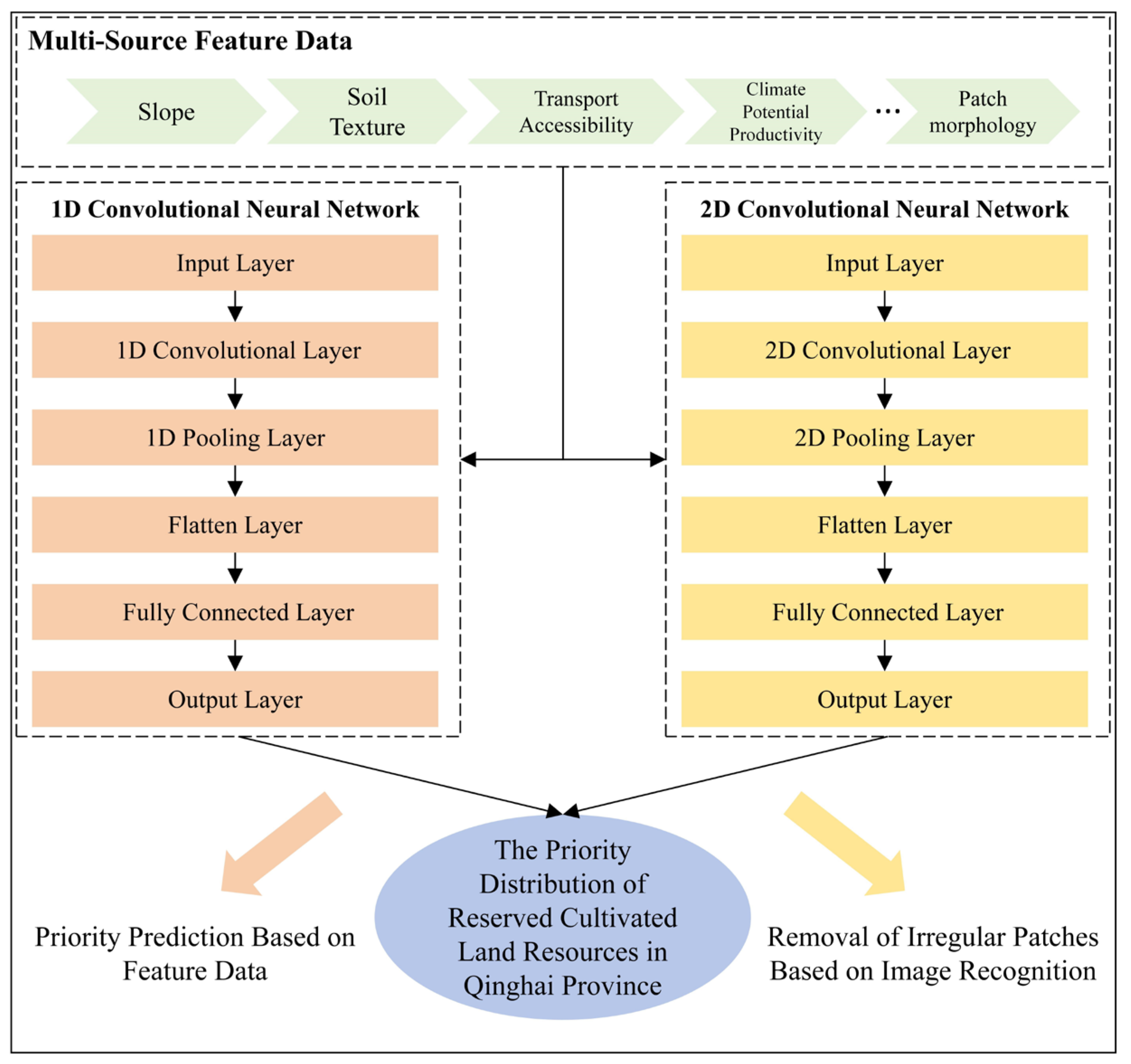
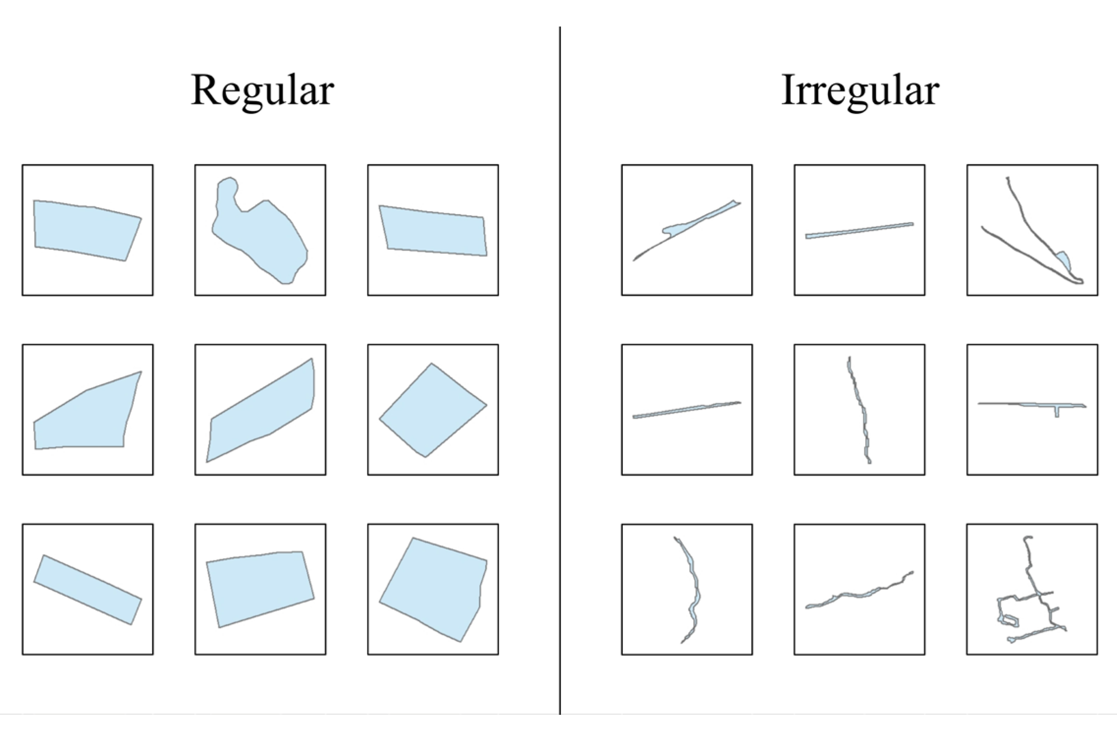
The present study develops a dual-screening framework that integrates multi-source data evaluation with patch-morphology verification (Figure 2). This intelligent-selection framework for reserved cultivated land resources comprises two main components: (1) Multi-source feature data—such as slope, soil texture, transportation accessibility, and climate potential productivity (CPP)—are consolidated and used as inputs. A trained 1D-CNN model then extracts deep feature representations and predicts a priority score for each reserved cultivated land patch, producing a ranked list of development priorities. (2) The vector patches of reserved cultivated land resources are converted into two-dimensional images to capture their spatial morphology. A trained 2D-CNN model analyzes these patch images to detect irregular patches, classifying each as either regular or irregular with respect to agricultural suitability. Finally, the outputs are integrated by removing patches identified as irregular by the 2D-CNN, ensuring that only morphologically suitable patches are retained for priority analysis.

2.3.1. Indicator Construction

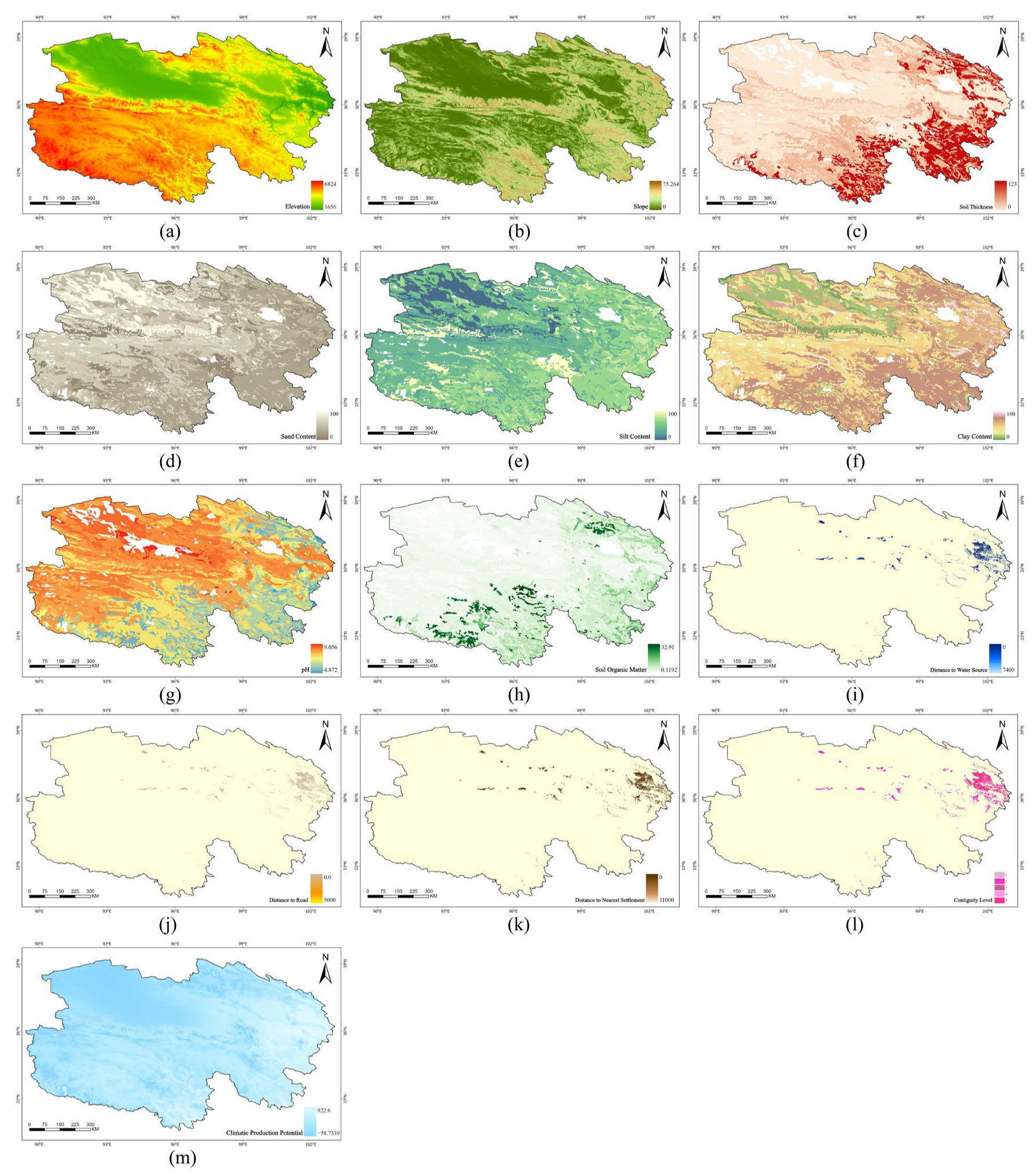
We selected eleven quantitative indicators, categorized into three groups—natural, economic, and climatic—including elevation, slope, effective soil-layer thickness, soil texture, soil pH, soil organic-matter content, irrigation conditions, transportation accessibility, cultivation accessibility, contiguity, and CPP. Using ArcGIS Pro (version 3.0.1, licensed via an institutional License Manager), we produced the spatial distribution maps of these indicators, as shown in Figure 3.

Natural factors comprise seven quantitative indicators: elevation, slope, effective soil-layer thickness, soil texture, soil pH, soil organic-matter content, and irrigation conditions. The classification criteria are primarily based on national technical standards and regulations, including the Technical Regulations for the Investigation and Evaluation of Reserved Cultivated Land Resources and the Technical Standards for Cultivated Land Quality Evaluation. Their definitions, implications, and scoring rules are as follows:

(1)

Elevation: vertical height above sea level. Higher elevations correspond to lower temperatures, larger diurnal ranges, and shorter growing seasons, which hinder crop growth. Scoring rules: <2500 m = 10; 2500–3200 m = 6; 3200–3800 m = 4; ≥3800 m = 2.

(2)

Slope: terrain inclination. Slope is closely related to soil erosion [45], and values above certain thresholds increase the difficulty and risk of mechanized farming. Scoring rules: 0–2° = 10; 2–6° = 8; 6–15° = 6; 15–25° = 4.

(3)

Effective Soil-Layer Thickness: depth available for root growth and water storage. Thicker soil layers favor root development and moisture retention. Scoring rules: ≥50 cm = 10; 30–50 cm = 6; <30 cm = 4.

(4)

Soil Texture: relative proportions of sand, silt, and clay. Loam provides an optimal balance for crop growth. Scoring rules: loam, light loam = 10; sandy loam, heavy loam = 6; sand, clay = 4.

(5)

Soil pH: soil acidity/alkalinity. Neutral to mildly acidic soils promote nutrient availability and microbial activity. Scoring rules: pH 5.5–7.5 = 10; 7.5–8.5 = 6; >8.5 = 4.

(6)

Soil Organic-Matter Content: proportion of decomposed residues and microbial biomass. Higher levels improve fertility, soil structure, aeration, and water retention. Scoring rules: ≥8% = 10; <8% = 6.

(7)

Irrigation Conditions: distance from a field patch to the nearest water source, calculated in ArcGIS. Shorter distances enable more reliable irrigation. As no unified national criterion is available, classification was conducted using the natural breaks method. Scoring rules: <600 m = 10; 600–1200 m = 8; ≥1200 m = 6.

Economic factors include three indicators: transportation accessibility, cultivation accessibility, and contiguity. The first two were classified using the natural breaks method, while contiguity followed the national evaluation standards.

(1)

Transportation Accessibility: distance from a field patch to major transport networks (e.g., township or county roads). Closer proximity and better road conditions reduce transport costs and losses. Distance to the nearest road was calculated in ArcGIS. Scoring rules: <100 m = 10; 100–300 m = 8; 300–500 m = 6; ≥500 m = 4.

(2)

Cultivation Accessibility: distance from a field patch to the nearest settlement, reflecting labor and management convenience. Distance to the nearest settlement was calculated in ArcGIS. Scoring rules: <100 m = 10; 100–700 m = 8; 700–1300 m = 6; ≥1300 m = 4.

(3)

Contiguity: degree of spatial aggregation of adjacent patches. Higher contiguity supports large-scale farming, facilitates unified management and mechanization, and reduces costs. Contiguity was calculated in ArcGIS by aggregating patches, computing their area, and applying corrections. Plains: ≥900 m² = 10; 600–900 m² = 8; 400–600 m² = 6; 150–400 m² = 4; <150 m² = 2. Mountainous/Hilly areas: ≥400 m² = 10; 250–400 m² = 8; 150–250 m² = 6; 80–150 m² = 4; <80 m² = 2.

The CPP was estimated using the Thornthwaite Memorial model, as follows:

$$E_0=300+25t+0.05t^3$$

(1)

$$ET={\displaystyle \frac{1.05p}{\sqrt{1+{\left(\frac{1.05p}{E_0}\right)}^2}}}$$

(2)

$$CPP=30000\left(1-e^{-0.0009695(ET-20)}\right)$$

(3)

t: annual mean temperature (°C); p: annual precipitation (mm); $E_0$: annual potential evapotranspiration (mm); ET: annual actual evapotranspiration (mm); CPP: climate potential productivity (kg hm⁻² a⁻¹).

2.3.2. Sample-Set Preparation

For the 1D-CNN model, five-fold cross-validation was employed to ensure robustness and reduce sampling bias. The dataset of 12,000 samples was randomly partitioned into five equal subsets of 2400 samples each. In each iteration, four subsets (9600 samples) were used for training and one subset (2400 samples) for validation, with every subset serving as the validation set once. This strategy avoided reliance on a single train–validation split and yielded a more stable estimate of model performance. Five folds were selected as a compromise between computational efficiency and reliable estimation, given the relatively large sample size in this study.

For the 2D-CNN model, the dataset was randomly divided into training, validation, and test sets in a 4:1:1 ratio, resulting in 8000, 2000, and 2000 samples, respectively. To augment the training set and enhance the robustness of the irregular-patch removal model, data-augmentation techniques were applied, including random rotations of ±20°, scaling by factors of 0.8–1.2, and horizontal flips.

2.3.3. Data Normalization

Before feeding the input indicators into the neural networks, all continuous variables were normalized to the range [0, 1] using min–max scaling:

$$x_i^{\prime }={\displaystyle \frac{x_i-x_{min}}{x_{max}-x_{min}}}$$

(4)

$x_i$: the original value of the variable for the i-th observation; $x_{min}$: the minimum value of the variable; $x_{max}$: the maximum value of the variable; $x_i^{\prime }$: the normalized value of the variable for the i-th observation.

2.3.4. CNN Construction

The 1D-CNN designed for attribute indicators takes as input an 11-dimensional sequence. It contains two successive convolutional blocks: the first applies a one-dimensional convolution with 32 filters of size 3, followed by a ReLU activation and max-pooling with a stride of 2; the second applies a convolution with 64 filters of size 3, followed by ReLU and max-pooling. The extracted features are passed through two fully connected layers with 64 and 32 units, respectively, each with ReLU activations, and are finally mapped to a two-class softmax output.

The 2D-CNN for patch morphology takes grayscale rasterized images of patches as input. It consists of three convolutional blocks: the first with 32 filters of size 3 × 3, batch normalization, ReLU activation, and 2 × 2 max-pooling; the second with 64 filters of size 3 × 3, batch normalization, ReLU activation, and 2 × 2 max-pooling; and the third with 128 filters of size 3 × 3, followed by batch normalization and ReLU. A global average pooling layer reduces dimensionality before the final softmax classifier with two output units. Both models were trained using cross-entropy loss optimized with Adam. For the 1D-CNN, the initial learning rate was 0.001, the batch size was 32, and the maximum number of epochs was 100. For the 2D-CNN, the initial learning rate was 0.001, the batch size was 16, and the maximum number of epochs was 30. In the 2D-CNN, batch normalization and global average pooling served as regularization, while in the 1D-CNN, max-pooling and shallow network depth helped limit overfitting.

2.3.5. CNN Model Accuracy Validation

In this study, both the 1D-CNN and 2D-CNN models calculated accuracy using the following formula, with the final accuracy of the 1D-CNN model obtained as the average across five-fold cross-validation:

$$\mathit{Accuracy}={\displaystyle \frac{1}{N}}{\sum }_{i=1}^N\delta (\widehat{y_i},y_i)\times 100\%$$

(5)

N: the total number of samples in the validation set; $\widehat{y_i}$: the predicted label for the i-th sample; $y_i$: the true label for the i-th sample; $\delta$: the indicator function, which equals 1 when $\widehat{y_i}$ = $y_i$ and 0 otherwise.

After training the 2D-CNN model, a confusion matrix was used to visualize the distribution of errors between regular and irregular patches:

$$CM=\left. [\begin{array}{cc}TP& FP\\ FN& TN\end{array}\right]$$

(6)

TP (True Positive): number of correctly identified irregular patches. FP (False Positive): number of regular patches misclassified as irregular. FN (False Negative): number of irregular patches misclassified as regular. TN (True Negative): number of correctly identified regular patches.

To further evaluate the classification performance of the 2D-CNN model, particularly for the irregular class, the total classification error was decomposed into quantity error and allocation error based on the confusion matrix. This decomposition provides a more nuanced evaluation of the model’s ability to discriminate irregular patches, distinguishing between overall quantity misestimation and individual sample misclassification. Quantity error measures the systematic overestimation or underestimation of the irregular class and is calculated as the absolute difference between the predicted and actual numbers of positive samples:

$$Quantity Error=|\mathit{FP}-\mathit{FN}|$$

(7)

Allocation error represents the remaining misclassification after accounting for quantity error, reflecting sample-level misallocation between classes:

$$\mathit{Allocation}\mathit{Error}=Total Error-Quantity Error$$

(8)

To comprehensively evaluate the classification performance of the constructed CNN models, this study employed two widely used assessment tools: the Receiver Operating Characteristic (ROC) curve and the Precision–Recall (PR) curve. The corresponding summary metrics—Area Under the ROC Curve (AUC) and Average Precision (AP)—are calculated as follows:

$$AUC={\int }_0^{1}TPR\left({FPR}^{-1}\left(x\right)\right)dx$$

(9)

TPR (True Positive Rate): the proportion of all positive samples that are correctly identified as positive. FPR (False Positive Rate): the proportion of all negative samples that are incorrectly identified as positive.

$$\begin{array}{rr}& \\ & AP={\displaystyle \sum _{n=1}^N}\left(R_n-R_{n-1}\right)\cdot P_n\end{array}$$

(10)

N: the total number of samples; $P_n$: the precision of the n-th sample after sorting all samples in descending order by their predicted scores; $R_n$: the recall of the n-th sample after the same ordering.

2.3.6. CNN Model Outputs

To quantify the development priority of each patch, the model incorporates a Softmax mechanism into the output layer of the 1D-CNN, producing a probability distribution. The network’s final layer is a fully connected layer with two neurons, producing an output vector z = [ $z_0,z_1$ ], where $z_0\mathrm{a}\mathrm{n}\mathrm{d}{z}_1$ are the unnormalized scores (logits) for the “non-priority” and “priority” classes, respectively. After model training, the predict function in the Deep Learning Toolbox was used to perform forward inference on the dataset and obtain the class-probability distributions. The Softmax layer then transforms z into a valid probability distribution:

$$p_i={\displaystyle \frac{exp\left(z_i\right)}{\sum _{j=0}^{1}exp\left(z_j\right)}}, i=0, 1$$

(11)

$p_i$: the probability that a sample belongs to the “priority development” class; $z_i$: the raw activation (logit) produced by the i-th neuron in the network’s output layer; $z_j$: the raw activation (logit) produced by the neuron corresponding to class j in the output layer.

When discriminating irregular patches with the 2D-CNN model, the classify function from the Deep Learning Toolbox was used to perform inference on the dataset. This function takes the preprocessed image datastore and the trained network as inputs, and outputs a predicted class label for each image. As with the 1D-CNN, the final layer is a fully connected layer with two neurons—one for regular patches and one for irregular patches—followed by a Softmax function that converts the unnormalized scores into a probability distribution. Finally, the classification layer selects the class with the highest Softmax probability as the model prediction.

2.3.7. SHAP Analysis

To enhance the interpretability of the 1D-CNN model, this study introduces Shapley additive explanations (SHAP) values to explain the model output. SHAP is a game-theoretic approach based on Shapley values that quantifies the marginal contribution of each input feature to the model prediction, thereby revealing the model’s decision-making mechanism. Its mathematical definition is as follows:

$${\varphi }_i\left(f,x\right)=\sum _{S\subseteq F\backslash \left\{i\right\}}{\displaystyle \frac{\left|S\right|!\left(\left|F\right|-\left|S\right|-1\right)!}{\left|F\right|!}}\left. [f\left(S\cup \left\{i\right\}\right)-f\left(S\right)\right]$$

(12)

${\varphi }_i\left(f,x\right)$: the marginal contribution of feature i to the prediction of model f for input x; F: the set of all input features; S: a subset that does not include feature i; f(S): the model’s output when only the features in subset S are present; $\left|S\right|$: the number of features in subset S; $\left|F\right|$: the total number of features.

2.3.8. Ablation Study

To further verify the contribution of each indicator to model performance, ablation experiments were conducted. In this procedure, each indicator was removed from the input feature set in turn, while the remaining conditions were kept unchanged, and the 1D-CNN model was retrained. Model performance was then evaluated on the same dataset, with accuracy, area under the ROC curve (AUC), and average precision (AP) recorded and compared against the full-feature model. In this way, the effect of excluding a single indicator on prediction performance could be quantitatively assessed, providing supplementary validation of the interpretability results obtained from SHAP analysis.

2.3.9. Baseline Method: AHP

To provide a traditional baseline for comparison with the CNN-based models, this study employed the AHP. AHP decomposes a complex multi-criteria evaluation into a hierarchical structure of goals, criteria, and indicators, and quantifies the relative importance of the indicators through pairwise comparison matrices. The indicator system is consistent with that of the CNN models, as shown in

Table 1. Indicator weights used in the AHP method.

Indicator	Weight
Elevation	0.0577
Slope	0.1346
Soil thickness	0.0962
Soil texture	0.0577
Soil pH	0.0385
Organic matter	0.0577
Irrigation conditions	0.1346
Cultivation accessibility	0.0962
Transport accessibility	0.0769
Contiguity	0.1154
CPP	0.1346

. The weights were determined by combining expert consultation with relevant technical guidelines. Consistency checks confirmed that the constructed judgment matrix satisfied the condition CR < 0.10, indicating reliable weight assignments.

In terms of data input, the AHP method used exactly the same dataset and 11 evaluation indicators as the CNN models. The overall priority score of each reserved cultivated land patch is calculated as follows:

$$S=\sum _{i=1}^n{w}_i\cdot x_i$$

(13)

$w_i$: the indicator weight determined by AHP; $x_i$: the normalized indicator score; n: the total number of indicators.

3. Results

3.1. Priority-Ranking Results for Reserved Cultivated Land Resources in Qinghai Province

The model-generated priority scores were classified into five levels using the natural-breaks method: Level 1 represents the highest priority and greatest suitability for development, whereas Level 5 represents the lowest priority, reflecting high development difficulty or limited potential. By integrating the priority-scoring results with irregular-patch identification, Figure 4 presents three representative patch examples. The first two are morphologically regular patches with favorable natural conditions, assigned to priority Levels 1 and 2, respectively. The third is identified as irregular by the 2D-CNN and therefore classified as Level 5, indicating unsuitability for development.

For regional analysis, Qinghai Province was divided into eastern, central, southern, and western zones according to geography and administrative boundaries. From Figure 5, it can be seen that in the eastern zone, approximately 64% of reserved cultivated land resources are classified as Level 1, followed by 27% in the central zone, while the western and southern zones account for only 7% and 3%, respectively. This distribution indicates that eastern Qinghai has the highest overall quality and development potential. Level 2 resources exhibit a bipolar distribution, with about 45% in the east and nearly 38% in the west, whereas the central zone contains 17% and the southern zone less than 1%. Nearly all medium-priority resources (Levels 2–3) are located in the western zone, with the other zones collectively accounting for less than 7%, demonstrating the concentration of moderate-potential reserves in the west. Low-priority resources (Levels 4–5) are also concentrated in the west—Levels 4 and 5 account for approximately 18.8% and 33.9% of the provincial total, respectively—whereas the eastern and central zones together contribute less than 30%, and the southern zone is negligible.

Overall, Levels 1–5 constitute about 11.8%, 8.3%, 27.1%, 18.8%, and 33.9% of the total reserved cultivated land area, respectively. High-priority resources (Levels 1–2) together account for roughly 20.1%, medium priority (Level 3) forms the largest share at 27.1%, and low-priority resources (Levels 4–5) comprise 52.7%, indicating that more than half of the province’s reserves face relatively high development challenges or limited potential.

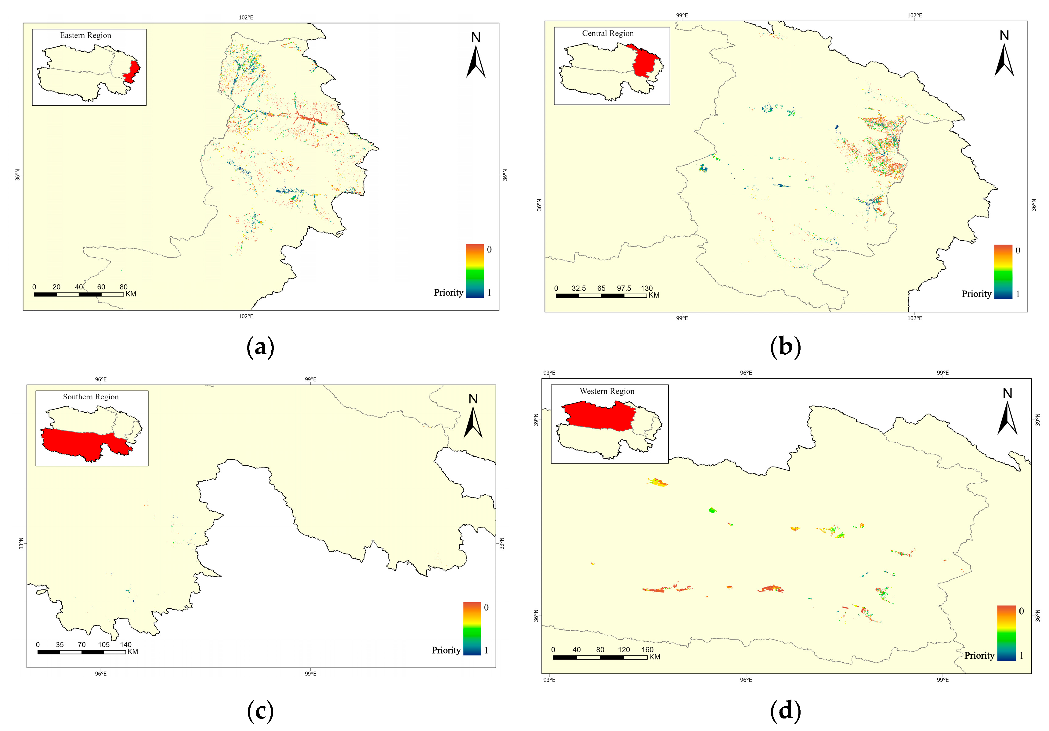
Figure 6 highlights the marked spatial imbalance in the priority distribution of reserved cultivated land resources in Qinghai. The eastern and central zones are dominated by high-priority resources, reflecting their gentle terrain, relatively abundant water resources, and existing agricultural infrastructure. Although the western zone is rich in reserve resources, it is dominated by medium- to low-priority areas. Its location in the hinterland of the Tibetan Plateau, with an arid climate, scarce precipitation, and severe land desertification, results in generally low priority, with only isolated high-priority patches near irrigation districts. The southern zone, constrained by high elevation and a cold climate, has limited resource quantity and development potential.

From the perspective of irregular patch elimination, irregularly shaped patches account for approximately 6.95% of the total provincial area, indicating a substantial proportion of morphological anomalies at this scale. Therefore, incorporating patch morphology into the evaluation of reserved cultivated land resources is essential.

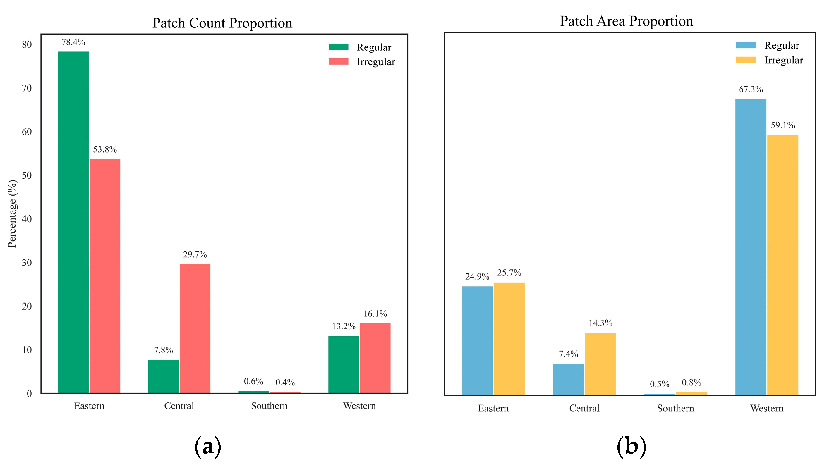
As shown in Figure 7, the eastern region accounts for 53.77% of the eliminated patch count but only 25.73% of the eliminated area, indicating a high patch density and the prevalence of fragmented, irregularly shaped small patches. The central region contributes 29.71% of the eliminated patches and 14.32% of the eliminated area, suggesting that most irregular patches here are small-to-medium in size. In the southern region, the eliminated patch count and area account for only 0.38% and 0.84%, respectively, indicating that although reserved cultivated land resources are scarce, their shapes are generally more regular. In contrast, the western region contributes 16.14% of the eliminated patches but 59.10% of the eliminated area, suggesting that this region contains abundant reserved cultivated land resources. Its complex natural terrain and fragmented development conditions result in the prevalence of large irregularly shaped patches.

3.2. Performance of the CNN Models in the Evaluation

Figure 8a,b presents the training and validation accuracy curves for the 1D-CNN and 2D-CNN models, respectively. For the 1D-CNN model, a five-fold cross-validation strategy was employed, and the curves represent the average training and validation accuracy across folds. The model converged rapidly during training, reaching a validation accuracy of 98.48% after 100 epochs, indicating that the selected features and network architecture effectively captured the intrinsic patterns of patch development priority. The trained model was then used to predict on the test set, assigning each patch a priority probability—higher values denoting greater development potential.

The 2D-CNN model converged on the validation set after approximately 30 epochs, achieving an overall classification accuracy of 91.95%. From the confusion matrix in Figure 9, where TP = 392, FN = 59, FP = 102, and TN = 1447, the irregular class attained a precision of 79.35% and a recall of 86.86%. This indicates that although most irregular patches were successfully identified, some regular patches were misclassified, reflecting a tendency to overestimate the irregular class. Decomposition of the total error of 161 samples reveals a quantity error of 43, corresponding to systematic overprediction of the irregular category, and an allocation error of 118, reflecting misclassification even after correcting for class totals. Although the overall accuracy is largely driven by correct recognition of regular patches, the model demonstrates a strong ability to discriminate irregular patches despite this bias. Importantly, such overprediction is acceptable in the context of reserved cultivated land resource development, where excluding additional potentially anomalous patches is preferable to retaining morphologically irregular ones. In this sense, the conservative tendency of the model ensures that the patches retained are more consistent in shape and structure with cultivated land characteristics.

Figure 10a,b presents the ROC and PR curves of the CNN and AHP methods. The ROC curve of the CNN model almost perfectly hugs the upper-left corner, with an AUC of 0.997. When the FPR is still below 0.05, the TPR has already approached 0.99, reaching 1.0 as the FPR increases to the range of 0.10–0.20. This demonstrates the model’s ability to capture positive samples accurately while maintaining an extremely low false positive rate. The corresponding PR curve further supports this result, with an AP of 0.995. At a recall of approximately 0.2, precision is already close to 0.99; as recall increases to 0.5, precision nearly reaches 1.0 and remains stably high within the range of 0.7–0.9. Even under the extreme case of full recall (1.0), precision remains at a reasonable level, demonstrating that the CNN model possesses robust discriminative capacity across different recall levels.

In contrast, the AHP method performs markedly worse, with an AUC of 0.841 and an AP of 0.865. Its ROC curve deviates substantially from the ideal upper-left corner, indicating larger errors in distinguishing between positive and negative classes. Similarly, its PR curve shows a sharp decline in precision at higher recall levels, suggesting difficulty in simultaneously maintaining high precision and recall. These results indicate that the CNN model has significant advantages in the priority selection of reserved cultivated land resources, as it achieves more accurate and stable identification of priority patches under a complex multidimensional indicator system, whereas the traditional weight-based AHP method is limited in capturing nonlinear patterns and exploiting feature interactions.

Figure 10c shows the ROC curve for the 2D-CNN model, with an AUC of 0.989. The curve climbs steeply, reaching TPR ≈ 0.94 while FPR is still below 0.05, rising to 0.99 at FPR ≈ 0.10, and approaching 1.0 when FPR reaches 0.20—ultimately hugging the upper-left corner. This indicates that the model maintains strong discriminative capacity, maximizing true positives while keeping false positives extremely low. Figure 10d presents the corresponding PR curve, with an AP of 0.908. Precision remains at 1.0 when recall is around 0.2, then falls to about 0.70 at recall = 0.5. It recovers to 0.88 at recall = 0.7 and remains at 0.85 at recall = 0.8. However, once recall exceeds 0.9, precision drops to about 0.75 and declines sharply to around 0.10 at full recall. This pattern suggests that the model sustains a good precision–recall balance across moderate recall levels, but faces a clear trade-off in precision when operating at very high recall.

Figure 11 confirms that the models accurately distinguish regular from irregular reserved cultivated land resource patches, providing a crucial complement to the selection system. The removal of irregular patches yields a more morphologically homogeneous candidate pool, reduces downstream analysis and manual review efforts, and enhances the overall accuracy and efficiency of the high-quality reserved cultivated land selection process.

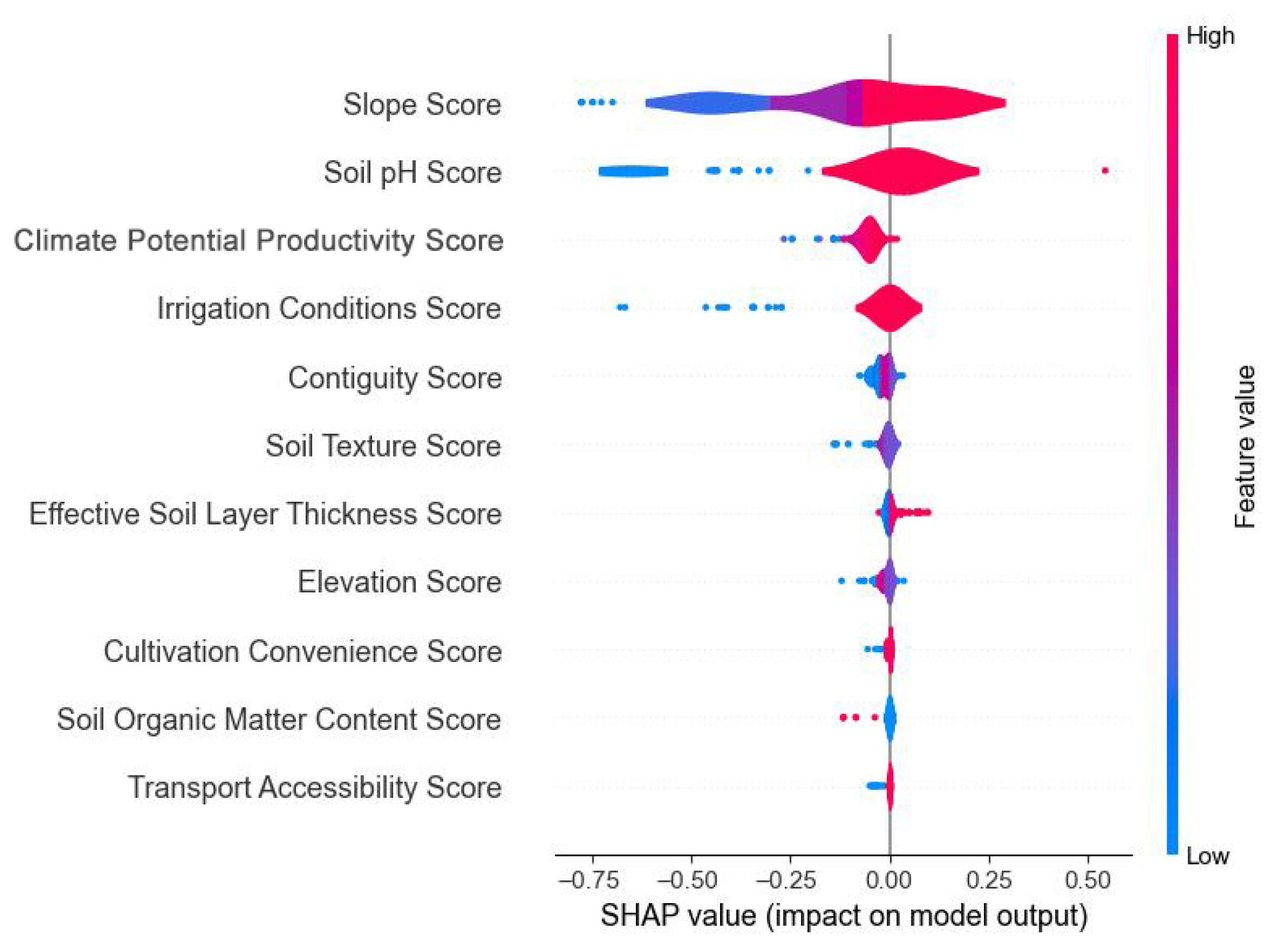
Figure 12 presents the SHAP summary plot in violin format, displaying the kernel-density distributions of the contributions of eleven features to the 1D-CNN model’s “priority probability” output. Slope emerges as the most influential feature: higher slope scores correspond to positive SHAP values, indicating that gentler slopes yield higher development priority. Soil pH ranks second, with higher pH scores clustering on the positive side, indicating that values closer to neutral increase development priority. CPP ranks third—its SHAP distribution is relatively concentrated, but higher CPP scores still tend toward positive contributions. Irrigation-condition scores rank fourth, exhibiting a roughly symmetric distribution with a slight positive bias, meaning that better irrigation access positively influences the model output. Contiguity scores occupy fifth place, with balanced contributions at both ends, suggesting that contiguity must be interpreted in conjunction with other factors. The remaining six features—soil texture, effective soil-layer thickness, elevation, cultivation accessibility, soil organic-matter content, and transportation accessibility—follow in descending order. Their SHAP distributions are narrower, indicating smaller individual contributions, yet they still fine-tune the priority ranking.

More importantly, the final prioritization is not determined by isolated factors but is jointly shaped by the interactions among multiple attributes. For instance, gentle slopes significantly enhance development priority only when accompanied by sufficient soil depth and favorable soil texture, reflecting a topography–soil coupling effect. Soils closer to neutral pH exert stronger positive impacts when organic-matter content is also relatively high, indicating a synergy between soil chemical properties and fertility. Likewise, the advantages of irrigation are further amplified when combined with transportation accessibility or cultivation convenience, highlighting the interaction between water availability and accessibility. Although contiguity shows relatively balanced marginal contributions, it functions as a spatial facilitator in areas where slope and soil conditions are favorable, reinforcing existing advantages. This demonstrates that the prioritization of reserved cultivated land resources arises from the combined effects of multiple factors.

To further validate these findings, ablation experiments were conducted by sequentially removing each indicator, and the results are summarized in

Table 2. Ablation experiment results: effect of removing individual indicators on model performance.

Setting	Mean Accuracy	Mean AUC	Mean AP	∆Accuracy	∆AUC	∆AP
Baseline (all)	0.9996	0.9999	0.9965	–	–	–
Drop Elevation	0.9997	1.0000	0.9979	+0.0001	+0.0000	+0.0014
Drop Slope	0.8668	0.8930	0.8842	−0.1328	−0.1070	−0.1124
Drop Soil pH	0.8641	0.9466	0.9563	−0.1355	−0.0534	−0.0402
Drop Soil thickness	0.9998	1.0000	0.9963	+0.0002	+0.0000	−0.0002
Drop Soil texture	0.9997	0.9998	0.9965	+0.0001	−0.0002	+0.0000
Drop Organic matter	0.9998	0.9998	0.9975	+0.0002	−0.0002	+0.0010
Drop Irrigation conditions	0.9669	0.9758	0.9726	−0.0327	−0.0242	−0.0239
Drop Cultivation accessibility	0.9992	1.0000	0.9982	−0.0004	−0.0000	+0.0017
Drop Transport accessibility	0.9994	1.0000	0.9969	−0.0002	−0.0002	+0.0003
Drop Contiguity	0.9998	1.0000	0.9986	+0.0002	+0.0000	+0.0021
Drop CPP	0.9998	1.0000	0.9972	+0.0002	+0.0000	+0.0007

The change values (ΔAccuracy, ΔAUC, ΔAP) are not applicable to the baseline model and therefore left blank.

. Most indicators exerted negligible influence, with accuracy changes within ±0.0004 when removed. In contrast, slope, soil pH, and irrigation conditions proved decisive for model performance. Excluding slope reduced accuracy by 0.133, accompanied by decreases of 0.107 in the area under the ROC curve and 0.112 in average precision, confirming its role as the most critical predictor. Removing soil pH reduced accuracy by 0.136, while excluding irrigation conditions lowered accuracy by 0.033. These results demonstrate that slope, soil pH, and irrigation conditions are the key indicators for determining the development priority of reserved cultivated land resources.

4. Discussion

4.1. Significance of the Priority Level of Reserved Cultivated Land Resources

The priority level of reserved cultivated land resources refers to the relative importance and order of different resources when they are developed into cultivated land. High-priority patches exhibit greater advantages in agricultural production potential, contiguity, accessibility to infrastructure, and other factors, making them more consistent with the requirements for the optimal spatial allocation of regional cultivated land resources. Classifying reserved cultivated land resources by priority level helps optimize land development and utilization decisions, guide differentiated management, and concentrate development efforts on higher-priority resources.

The evaluation logic adopted in this study is broadly consistent with current research, and the identified high-priority patches demonstrate strong reliability. Li et al. [46] applied a CNN–LSTM model coupled with the PLUS framework to simulate land-use optimization in Jilin Province. Their findings indicated that patches with more favorable soil conditions, accessibility, and contiguity exhibited higher agricultural production potential [46]. This outcome is consistent with our results, which show that high-priority patches are concentrated in areas with advantageous natural and infrastructural attributes. Likewise, Li et al. assessed the consolidation potential of saline–alkali reserved land resources using a two-level geographical unit division, revealing that priority development areas were concentrated in regions characterized by good contiguity and suitable ecological conditions [47]. Moreover, Wang et al., through an AHP-based evaluation in Haishu District of Ningbo City, reported that highly suitable patches generally possessed favorable accessibility, moderate slope, and sound soil fertility [21]. Collectively, these studies corroborate the logic underlying our prioritization: patches with higher scores in dimensions such as soil, slope, and irrigation consistently emerge as more promising for agricultural development.

Beyond these consistencies, this study introduces an additional methodological innovation by incorporating a patch-morphology verification step based on a 2D-CNN. Unlike the above studies, which primarily relied on indicator-based or simulation approaches, our framework explicitly excludes irregular or highly fragmented patches. This ensures that the final selection reflects not only strong agricultural development potential but also conformity with the practical requirements of mechanized cultivation and field layout. Such a dual-screening process enhances the applicability of the results for land-use planning.

4.2. Advantages of the Dual-Screening Model Framework

The dual-screening framework proposed in this study integrates a 1D-CNN and a 2D-CNN, targeting both attribute indicators and spatial morphology to fully exploit complementary features from multi-source heterogeneous data. The 1D-CNN excels at extracting features such as spectral sequences or one-dimensional attributes, while the 2D-CNN is adept at learning spatial textures and structural information from imagery, making the two approaches mutually reinforcing [48]. In this study, the 1D-CNN module takes vector-based attribute indicators of patches as input and, through multiple layers of one-dimensional convolution and pooling operations, efficiently uncovers nonlinear relationships within attribute sequences to accurately predict development priority. The 2D-CNN module converts vector patches into images to extract spatial morphology features—such as boundary regularity and shape integrity—automatically identifying and removing morphologically irregular patches (e.g., fragmented, jagged, or discontinuous edges) that are unsuitable for agricultural use. By reducing manual threshold setting and expert interpretation, this deep-learning pipeline significantly improves analysis efficiency and minimizes subjective bias. Furthermore, the framework’s modular design allows for seamless integration of additional attribute or image channels, making it adaptable to various regional scales and assessment requirements.

Beyond methodological advantages, the proposed framework also has strategic implications for sustainable land management. By enhancing the accuracy of priority selection for reserved cultivated land resources, it provides a reliable technical basis for timely supplementing arable land and stabilizing the farmland red line, thereby strengthening food security strategies under growing urbanization pressure. Meanwhile, the capacity to identify and exclude unsuitable or low-efficiency patches reduces the likelihood of farmland being converted into marginal land with limited productive capacity. This helps mitigate conflicts between agricultural protection and residential land expansion, enabling a more balanced allocation of land resources between food production and housing development. In this way, the framework not only improves evaluation precision but also informs policy decisions that reconcile agricultural security with urban development needs.

4.3. Limitations and Prospects

The proposed dual-screening framework demonstrates superior performance in the priority selection of reserved cultivated land resources, with notable advantages in accuracy, efficiency, and multi-source data fusion. Its accuracy and stability surpass those of traditional methods, providing a more scientific and intelligent approach to priority ranking and morphological filtering. Nonetheless, several areas warrant further refinement: (1) Regional transferability requires validation. Deep-learning models typically demand large, uniformly distributed training samples to avoid overfitting and enhance generalization [49]. Although this study’s models exhibit excellent adaptability to Qinghai’s high-altitude environment, performance may fluctuate in regions with differing terrain and climatic conditions due to variations in training-sample distribution and scale. Research shows that models trained solely on local data often suffer performance degradation when applied to different regions [50]. Future work could therefore include systematic validation across regions with contrasting edaphoclimatic conditions. Pilot studies could be conducted in representative environments such as low-altitude plains, semi-arid plateaus, and humid valleys, where independent datasets on soil quality, climatic factors, and land-use status are available. By comparing the framework’s predicted priority patterns with these independent evaluations, the robustness and generalization of the model could be more reliably assessed. In parallel, to bolster cross-region generalization, future work could explore transfer learning, domain adaptation, or multi-source pre-training strategies, combined with few-shot fine-tuning methods [51]. (2) Dynamic data and temporal changes are not addressed. This study is based on static geographic, topographic, and morphological data, without incorporating temporal dynamics. The suitability of reserved cultivated land exhibits seasonal fluctuations and long-term evolution; integrating dynamic data—such as meteorological factors and irrigation water usage—would enable continuous monitoring and evaluation, thereby supporting rapid decision-making under varying cropping periods, extreme weather events, or policy shifts. (3) The 2D-CNN model shows a tendency toward over-prediction of irregular patches. While this conservative bias ensures that most morphologically anomalous patches are excluded, thereby reducing the risk of retaining unsuitable plots, it also leads to the inadvertent removal of some regular patches. Such overestimation increases allocation error and may reduce the overall availability of candidate land resources. In practical applications, this trade-off is acceptable to a certain degree—since eliminating anomalous patches is preferable to mistakenly including unsuitable ones—but further optimization is needed to balance precision and recall. Future research could consider cost-sensitive learning, sample rebalancing, or threshold adjustment strategies to mitigate systematic over-prediction while maintaining the robustness of anomaly detection.

The multi-source data evaluation and patch-morphology verification framework developed in this study is not only applicable to reserved cultivated land selection but also holds promise in broader environmental and ecological contexts: (1) Wetland conservation and restoration. Wetland ecosystems involve complex hydrological conditions and diverse habitats [52]. Traditional wetland assessments rely heavily on field surveys or single indicators; by integrating multi-source spatiotemporal features such as water depth, vegetation cover, and wetland connectivity, the framework could use 1D-CNN to predict restoration priority and 2D-CNN to exclude anthropogenically disturbed or morphologically anomalous areas, enabling intelligent selection of conservation units. (2) Precision integrated water-fertilizer management. As agriculture moves toward efficiency and sustainability, precision agriculture technologies—driven by accurate monitoring and intelligent decision-making—optimize field water and fertilizer allocation [53]. Incorporating indicators like soil moisture, meteorological data, and vegetation indices, the framework can automate priority assessments for field water-fertilizer scheduling and, by excluding non-crop areas (e.g., roads, canals) via vector-based filtering, provide decision support for smart-agriculture platforms to achieve water and fertilizer savings while enhancing productivity. (3) Urban green space and ecological corridor planning. In urbanization, green-space systems and ecological corridors mitigate heat-island effects, improve air quality, and maintain ecological connectivity [54]. The framework can integrate factors such as population density, heat-island intensity, and pollution indices into a 1D-CNN predictor, then apply a 2D-CNN to remove built-environment patches, thereby accurately identifying candidate green-space zones.

5. Conclusions

The multi-source feature-fusion and machine-learning–driven dual-screening framework developed in this study leverages a 1D-CNN for priority prediction and a 2D-CNN for patch-morphology filtering. After 100 iterations, the 1D-CNN achieved a validation accuracy of 98.48%, demonstrating its ability to capture the combined influence of multiple indicators—such as patch area, slope, contiguity, and irrigation conditions—on development potential. The 2D-CNN, trained for approximately 30 epochs, reached a classification accuracy of 91.95% on the validation set, effectively removing morphologically anomalous patches and significantly enhancing data quality and the reliability of subsequent evaluations. These results indicate that the proposed framework offers substantial technical advantages and application potential for the quantitative evaluation and intelligent selection of reserved cultivated land resources, although the identification of high-potential areas should be further validated through field investigations, particularly analyses of soil physical and chemical properties, before conversion to cultivated land.

Using the complex plateau environment of Qinghai Province as a case study, this research conducted an in-depth analysis of the spatial distribution of reserved cultivated land priorities. The findings reveal that high-priority patches are predominantly clustered in the eastern and central regions, while medium- and low-priority resources are more common in the western region; the southern region exhibits both the smallest quantity and lowest development potential. This spatial pattern closely reflects Qinghai’s terrain, climatic conditions, and water-resource distribution. The case-study validation confirms the framework’s reliability in a typical, ecologically complex area and provides a solid foundation for its transferability to similar regions.

References

1. Wu, Y.; Shan, L.; Guo, Z.; Peng, Y. Cultivated Land Protection Policies in China Facing 2030: Dynamic Balance System versus Basic Farmland Zoning. Habitat Int. 2017, 69, 126–138. [Google Scholar] [CrossRef]
2. Yuan, X.; Shao, Y.; Li, Y.; Liu, Y.; Wang, Y.; Wei, X.; Wang, X.; Zhao, Y. Cultivated Land Quality Improvement to Promote Revitalization of Sandy Rural Areas along the Great Wall in Northern Shaanxi Province, China. J. Rural Stud. 2022, 93, 367–374. [Google Scholar] [CrossRef]
3. Zhou, Y.; Li, X.; Liu, Y. Cultivated Land Protection and Rational Use in China. Land Use Policy 2021, 106, 105454. [Google Scholar] [CrossRef]
4. Zhou, Y.; Chen, T.; Feng, Z.; Wu, K. Identifying the Contradiction between the Cultivated Land Fragmentation and the Construction Land Expansion from the Perspective of Urban-Rural Differences. Ecol. Inform. 2022, 71, 101826. [Google Scholar] [CrossRef]
5. Zhou, Y.; Zhong, Z.; Cheng, G. Cultivated Land Loss and Construction Land Expansion in China: Evidence from National Land Surveys in 1996, 2009 and 2019. Land Use Policy 2023, 125, 106496. [Google Scholar] [CrossRef]
6. Ariken, M.; Zhang, F.; Chan, N.w.; Kung, H.-t. Coupling Coordination Analysis and Spatio-Temporal Heterogeneity between Urbanization and Eco-Environment along the Silk Road Economic Belt in China. Ecol. Indic. 2021, 121, 107014. [Google Scholar] [CrossRef]
7. Chai, C.; Zhang, B.; Li, Y.; Niu, W.; Zheng, W.; Kong, X.; Yu, Q.; Zhao, M.; Xia, X. A New Multi-Dimensional Framework Considering Environmental Impacts to Assess Green Development Level of Cultivated Land during 1990 to 2018 in China. Environ. Impact Assess. Rev. 2023, 98, 106927. [Google Scholar] [CrossRef]
8. Feng, X.; Lin, X.; Li, Y.; Yang, J.; Yu, E.; He, C.; Lei, K.; Gao, W. Impact of Urban Land Development on Carbon Emission Performance Based on a Multidimensional Framework. Environ. Impact Assess. Rev. 2024, 105, 107429. [Google Scholar] [CrossRef]
9. Huang, Z.; Du, X.; Castillo, C.S.Z. How Does Urbanization Affect Farmland Protection? Evidence from China. Resour. Conserv. Recycl. 2019, 145, 139–147. [Google Scholar] [CrossRef]
10. Chen, L.; Song, G.; Meadows, M.E.; Zou, C. Spatio-Temporal Evolution of the Early-Warning Status of Cultivated Land and Its Driving Factors: A Case Study of Heilongjiang Province, China. Land Use Policy 2018, 72, 280–292. [Google Scholar] [CrossRef]
11. Wang, X.; Feng, Q.; Li, B.; Fan, Y.; Fan, H.; Yang, N.; Quan, Y.; Ding, H.; Zhang, Y. Trends and Factors Influencing the Evolution of Spatial Patterns of Cropland toward Large-Scale Agricultural Production in China. Land 2024, 13, 607. [Google Scholar] [CrossRef]
12. AbdelRahman, M.A.E.; Shalaby, A.; Essa, E.F. Quantitative Land Evaluation Based on Fuzzy-Multi-Criteria Spatial Model for Sustainable Land-Use Planning. Model. Earth Syst. Environ. 2018, 4, 1341–1353. [Google Scholar] [CrossRef]
13. Kuang, B.; Han, J.; Lu, X.; Zhang, X.; Fan, X. Quantitative Evaluation of China’s Cultivated Land Protection Policies Based on the PMC-Index Model. Land Use Policy 2020, 99, 105062. [Google Scholar] [CrossRef]
14. Chaudhary, S.; Kumar, A.; Pramanik, M.; Negi, M.S. Land Evaluation and Sustainable Development of Ecotourism in the Garhwal Himalayan Region Using Geospatial Technology and Analytical Hierarchy Process. Environ. Dev. Sustain. 2022, 24, 2225–2266. [Google Scholar] [CrossRef]
15. Douglas, I. Climate Change, Flooding and Food Security in South Asia. Food Secur. 2009, 1, 127–136. [Google Scholar] [CrossRef]
16. Chou, J.; Dong, W.; Wang, S.; Fu, Y. Quantitative Analysis of Agricultural Land Use Change in China. Phys. Chem. Earth 2015, 87–88, 3–9. [Google Scholar] [CrossRef]
17. Wang, J.; Wang, S.; Zhou, C. Quantifying Embodied Cultivated Land-Use Change and Its Socioeconomic Driving Forces in China. Appl. Geogr. 2021, 137, 102601. [Google Scholar] [CrossRef]
18. Akinci, H.; Özalp, A.Y.; Turgut, B. Agricultural Land Use Suitability Analysis Using GIS and AHP Technique. Comput. Electron. Agric. 2013, 97, 71–82. [Google Scholar] [CrossRef]
19. Chivasaa, W.; Mutanga, O.; Biradarc, C. Mapping Land Suitability for Maize (Zea mays L.) Production Using GIS and AHP Technique in Zimbabwe. S. Afr. J. Geomat. 2022, 8, 265–281. [Google Scholar] [CrossRef]
20. Mishra, A.K.; Deep, S.; Choudhary, A. Identification of Suitable Sites for Organic Farming Using AHP & GIS. Egypt. J. Remote Sens. Space Sci. 2015, 18, 181–193. [Google Scholar] [CrossRef]
21. Wang, X.; Chai, L.; Zeng, S.; Su, J.; Ye, B.; Lü, H.; Chen, C.; Gong, J.; Liu, M.; Wang, X.; et al. Evaluating Cultivated Reserved Land Resources in a Highly Urbanized Region of China: A Case Study in Haishu District, Ningbo City. Land 2024, 13, 1444. [Google Scholar] [CrossRef]
22. Zabihi, H.; Ahmad, A.; Vogeler, I.; Said, M.N.; Golmohammadi, M.; Golein, B.; Nilashi, M. Land Suitability Procedure for Sustainable Citrus Planning Using the Application of the Analytical Network Process Approach and GIS. Comput. Electron. Agric. 2015, 117, 114–126. [Google Scholar] [CrossRef]
23. Malczewski, J.; Chapman, T.; Flegel, C.; Walters, D.; Shrubsole, D.; Healy, M.A. GIS Multicriteria Evaluation with Ordered Weighted Averaging (OWA): Case Study of Developing Watershed Management Strategies. Environ. Plan. A 2003, 35, 1769–1784. [Google Scholar] [CrossRef]
24. Montgomery, B.; Dragićević, S.; Dujmović, J.; Schmidt, M. A GIS-Based Logic Scoring of Preference Method for Evaluation of Land Capability and Suitability for Agriculture. Comput. Electron. Agric. 2016, 124, 340–353. [Google Scholar] [CrossRef]
25. Braimoh, A.K.; Vlek, P.L.G.; Stein, A. Land Evaluation for Maize Based on Fuzzy Set and Interpolation. Environ. Manag. 2004, 33, 226–238. [Google Scholar] [CrossRef]
26. Liu, Y.; Jiao, L.; Liu, Y.; He, J. A Self-Adapting Fuzzy Inference System for the Evaluation of Agricultural Land. Environ. Model. Softw. 2013, 40, 226–234. [Google Scholar] [CrossRef]
27. Reshmidevi, T.V.; Eldho, T.I.; Jana, R. A GIS-Integrated Fuzzy Rule-Based Inference System for Land Suitability Evaluation in Agricultural Watersheds. Agric. Syst. 2009, 101, 101–109. [Google Scholar] [CrossRef]
28. Jamil, M.; Sahana, M.; Sajjad, H. Crop Suitability Analysis in the Bijnor District, UP, Using Geospatial Tools and Fuzzy Analytical Hierarchy Process. Agric. Res. 2018, 7, 506–522. [Google Scholar] [CrossRef]
29. Tashayo, B.; Honarbakhsh, A.; Azma, A.; Akbari, M. Combined Fuzzy AHP–GIS for Agricultural Land Suitability Modeling for a Watershed in Southern Iran. Environ. Manag. 2020, 66, 364–376. [Google Scholar] [CrossRef]
30. LI, B.; ZHANG, F.; ZHANG, L.-W.; HUANG, J.-F.; JIN, Z.-F.; GUPTA, D.K. Comprehensive Suitability Evaluation of Tea Crops Using GIS and a Modified Land Ecological Suitability Evaluation Model. Pedosphere 2012, 22, 122–130. [Google Scholar] [CrossRef]
31. Feng, Y.; Li, H.; Tong, X.; Li, P.; Wang, R.; Chen, S.; Xi, M.; Sun, J.; Wang, Y.; He, H.; et al. Optimized Landing Site Selection at the Lunar South Pole: A Convolutional Neural Network Approach. IEEE J. Sel. Top. Appl. Earth Obs. Remote Sens. 2024, 17, 10998–11015. [Google Scholar] [CrossRef]
32. Tanoori, G.; Soltani, A.; Modiri, A. Predicting Urban Land Use and Mitigating Land Surface Temperature: Exploring the Role of Urban Configuration with Convolutional Neural Networks. J. Urban Plan. Dev. 2024, 150, 04024029. [Google Scholar] [CrossRef]
33. Liu, H.; Liu, J.; Yang, W.; Chen, J.; Zhu, M. Analysis and Prediction of Land Use in Beijing-Tianjin-Hebei Region: A Study Based on the Improved Convolutional Neural Network Model. Sustainability 2020, 12, 3002. [Google Scholar] [CrossRef]
34. Taghizadeh-Mehrjardi, R.; Nabiollahi, K.; Rasoli, L.; Kerry, R.; Scholten, T. Land Suitability Assessment and Agricultural Production Sustainability Using Machine Learning Models. Agronomy 2020, 10, 573. [Google Scholar] [CrossRef]
35. Zhu, X.; Xiao, G.; Wang, S. Suitability Evaluation of Potential Arable Land in the Mediterranean Region. J. Environ. Manag. 2022, 313, 115011. [Google Scholar] [CrossRef]
36. Zhu, X.; Li, N.; Pan, Y. Optimization Performance Comparison of Three Different Group Intelligence Algorithms on a SVM for Hyperspectral Imagery Classification. Remote Sens. 2019, 11, 734. [Google Scholar] [CrossRef]
37. Dang, K.B.; Burkhard, B.; Windhorst, W.; Müller, F. Application of a Hybrid Neural-Fuzzy Inference System for Mapping Crop Suitability Areas and Predicting Rice Yields. Environ. Model. Softw. 2019, 114, 166–180. [Google Scholar] [CrossRef]
38. Shastri, S.; Kumar, S.; Mansotra, V.; Salgotra, R. Advancing Crop Recommendation System with Supervised Machine Learning and Explainable Artificial Intelligence. Sci. Rep. 2025, 15, 25498. [Google Scholar] [CrossRef]
39. Zhong, L.; Guo, X.; Ding, M.; Ye, Y.; Jiang, Y.; Zhu, Q.; Li, J. SHAP Values Accurately Explain the Difference in Modeling Accuracy of Convolution Neural Network between Soil Full-Spectrum and Feature-Spectrum. Comput. Electron. Agric. 2024, 217, 108627. [Google Scholar] [CrossRef]
40. Hussein, E.E.; Zerouali, B.; Bailek, N.; Derdour, A.; Ghoneim, S.S.M.; Santos, C.A.G.; Hashim, M.A. Harnessing Explainable AI for Sustainable Agriculture: SHAP-Based Feature Selection in Multi-Model Evaluation of Irrigation Water Quality Indices. Water 2025, 17, 59. [Google Scholar] [CrossRef]
41. Pham, T.H.; Acharya, P.; Bachina, S.; Osterloh, K.; Nguyen, K.D. Deep-Learning Framework for Optimal Selection of Soil Sampling Sites. Comput. Electron. Agric. 2024, 217, 108650. [Google Scholar] [CrossRef]
42. Ganati, B.A.; Sitote, T.M. Predicting Land Suitability for Wheat and Barley Crops Using Machine Learning Techniques. Sci. Rep. 2025, 15, 15879. [Google Scholar] [CrossRef]
43. Reese, M.; Dasgupta, A.; Waske, B. Farmland Quality Assessment Using Deep Learning and UAVs. Remote Sens. Appl. Soc. Environ. 2024, 35, 101235. [Google Scholar] [CrossRef]
44. Mohan, R.N.V.J.; Rayanoothala, P.S.; Sree, R.P. Next-Gen Agriculture: Integrating AI and XAI for Precision Crop Yield Predictions. Front. Plant Sci. 2024, 15, 1451607. [Google Scholar] [CrossRef]
45. Koulouri, M.; Giourga, C. Land Abandonment and Slope Gradient as Key Factors of Soil Erosion in Mediterranean Terraced Lands. Catena 2007, 69, 274–281. [Google Scholar] [CrossRef]
46. Li, S.; Zhang, C.; Chen, C.; Yang, C.; Zhao, L.; Bai, X. Optimization Simulation and Comprehensive Evaluation Coupled with CNN-LSTM and PLUS for Multi-Scenario Land Use in Cultivated Land Reserve Resource Area. Remote Sens. 2025, 17, 1619. [Google Scholar] [CrossRef]
47. Li, S.; Zhang, C.; Luo, C.; Li, S.; Yun, W.; Gao, B. Analysis of Comprehensive Land Consolidation in Cultivated Land Reserve Resource Areas Based on Two-Level Geographical Unit Division. Land 2024, 13, 470. [Google Scholar] [CrossRef]
48. Liu, J.; Wang, T.; Skidmore, A.; Sun, Y.; Jia, P.; Zhang, K. Integrated 1D, 2D, and 3D CNNs Enable Robust and Efficient Land Cover Classification from Hyperspectral Imagery. Remote Sens. 2023, 15, 4797. [Google Scholar] [CrossRef]
49. Chen, H.; He, G.; Peng, X.; Wang, G.; Yin, R. A Multi-Scale Feature Fusion Deep Learning Network for the Extraction of Cropland Based on Landsat Data. Remote Sens. 2024, 16, 4071. [Google Scholar] [CrossRef]
50. António, V.; Kimani, G.; Umohoza, E.; Busogi, M. Cross-Regional Transferability of AI Crop-Type Mapping: Insights and Challenges. In Proceedings of the 2024 International Conference on Information Technology for Social Good, Bremen, Germany, 4–6 September 2024; ACM: New York, NY, USA, 2024; pp. 453–461. [Google Scholar]
51. Karakullukcu, E. Leveraging Convolutional Neural Networks for Image-Based Classification of Feature Matrix Data. Expert Syst. Appl. 2025, 281, 127625. [Google Scholar] [CrossRef]
52. Zhao, Q.; Bai, J.; Huang, L.; Gu, B.; Lu, Q.; Gao, Z. A Review of Methodologies and Success Indicators for Coastal Wetland Restoration. Ecol. Indic. 2016, 60, 442–452. [Google Scholar] [CrossRef]
53. Lin, N.; Wang, X.; Zhang, Y.; Hu, X.; Ruan, J. Fertigation Management for Sustainable Precision Agriculture Based on Internet of Things. J. Clean. Prod. 2020, 277, 124119. [Google Scholar] [CrossRef]
54. Wu, B.; Bao, Y.; Wang, Z.; Chen, X.; Wei, W. Multi-Temporal Evaluation and Optimization of Ecological Network in Multi-Mountainous City. Ecol. Indic. 2023, 146, 109794. [Google Scholar] [CrossRef]
Figure 1. Location of the Study Area.
Land 14 01931 g001
Figure 2. Methodological Framework.
Land 14 01931 g002
Figure 3. Spatial Distribution Maps of Indicator Parameters in the Intelligent Selection Framework for Reserved Cultivated Land Resources in Qinghai Province. (a) Elevation; (b) Slope; (c) Effective soil-layer thickness; (d) Relative proportion of soil sand content; (e) Relative proportion of soil silt content; (f) Relative proportion of soil clay content; (g) Soil pH; (h) Soil organic matter content; (i) Irrigation conditions; (j) Transportation accessibility; (k) Cultivation accessibility; (l) Contiguity; (m) Climatic production potential.
Land 14 01931 g003
Figure 4. Aerial Overview of Example Sample Patches. The blue lines indicate the selected example patches.
Land 14 01931 g004
Figure 5. Heatmap of Priority Level Distribution of Reserved Cultivated Land Resources Across Regions in Qinghai Province.
Land 14 01931 g005
Figure 6. Priority Level Distribution Map of Reserved Cultivated Land Resources Across Regions of Qinghai Province. (a) Distribution of priority levels in the eastern region; (b) Distribution of priority levels in the central region; (c) Distribution of priority levels in the southern region; (d) Distribution of priority levels in the western region.
Land 14 01931 g006
Figure 7. Proportional Comparison of Regular and Irregular Shaped Patches by Region in Qinghai Province. (a) Proportion of patch shapes by number in each region; (b) Proportion of patch shapes by area in each region.
Land 14 01931 g007
Figure 8. Training and Validation Accuracy Curves of the CNN Models. (a) Training and validation accuracy curves of the 1D-CNN model; (b) Training and validation accuracy curves of the 2D-CNN model.
Land 14 01931 g008
Figure 9. Confusion Matrix of the 2D-CNN Model.
Land 14 01931 g009
Figure 10. CNN Model Performance Evaluation: ROC and PR Curves. The dashed line in the ROC curves represents the reference line of a random classifier (no-discrimination line). (a) ROC curve of the 1D-CNN model; (b) PR curve of the 1D-CNN model; (c) ROC curve of the 2D-CNN model; (d) PR curve of the 2D-CNN model.
Land 14 01931 g010aLand 14 01931 g010b
Figure 11. Partial Results of the 2D-CNN Model.
Land 14 01931 g011
Figure 12. SHAP Violin Plot of Feature Importance for the 1D-CNN Model.
Land 14 01931 g012