Article

Evaluating Urban Heat Island Effects in the Southwestern Plateau of China: A Comparative Analysis of Nine Estimation Methods

1
School of Earth Science, Yunnan University, Kunming 650500, China
2
Institute of International Rivers and Eco-Security, Yunnan University, Kunming 650500, China
*
Author to whom correspondence should be addressed.
Land 2025, 14(1), 37; https://doi.org/10.3390/land14010037
Submission received: 2 December 2024 / Revised: 22 December 2024 / Accepted: 25 December 2024 / Published: 28 December 2024

Abstract

:
Surface urban heat island intensity (SUHII) is a critical indicator of the urban heat island (UHI) effect. However, discrepancies in estimation methods may introduce uncertainty in SUHII values. While previous studies have examined the responses of SUHII to different methods at large scales, further analysis is needed for plateau cities in southwestern China, which have complex geographical features. This study investigates the spatiotemporal patterns and influencing factors of SUHII in 200 plateau cities across southwestern China via nine estimation methods that incorporate rural ranges and elevation-based conditions. The results show that: (1) The annual average daytime and nighttime SUHII for these cities were 0.97 ± 0.78 °C (mean ± std) and 0.21 ± 0.87 °C, respectively. For 22% of the cities during the day and 26% at night, the choice of different SUHII estimation methods resulted in the transformation between a surface urban heat island (SUHI) and a surface urban cold island (SUCI) due to the exclusion of rural pixels more than ±50 m from the median urban elevation. Compared with other regions, high-altitude plateau cities exhibited a slightly lower daytime SUHII but a significantly higher nighttime SUHII because of the lower atmospheric pressure in plateau areas, which limits the conduction and retention of heat. Consequently, heat dissipates more quickly at night, increasing SUHII values. (2) The mean ΔSUHIIAD (absolute difference in SUHII values across methods) was 0.51 ± 0.01 °C during the day and 0.44 ± 0.02 °C at night. (3) In high-altitude plateau cities, for all methods, the correlation of the SUHII with influencing factors was stronger, highlighting their sensitivity to both environmental and anthropogenic influences. These results enhance our understanding of plateau UHI dynamics and highlight the importance of considering appropriate rural definitions for cities with varying geographical characteristics.

1. Introduction

Rapid urbanization has led to the urban heat island (UHI) effect, in which urban temperatures exceed surrounding rural area temperatures [1,2,3]. Higher urban temperatures can have negative impacts on the ecological environment and human health [4,5]. Therefore, the monitoring and managing of surface urban heat islands (SUHIs) is critical in urban thermal environment research [6,7,8,9]. Research into the spatiotemporal patterns of SUHIs can enhance our understanding of urban thermal dynamics.
In recent years, numerous studies have been conducted on the spatiotemporal evolution of SUHIs using thermal infrared remote sensing imagery. Studies have demonstrated that SUHIs exhibited significant spatiotemporal heterogeneity across various spatial scales (for example individual cities, regions, and global) and temporal scales (for example daily, yearly, and interannual) driven by the combined effects of the urban structure, background climate, and human activities [8]. This heterogeneity indicates distinct evolutionary characteristics [10,11,12,13,14,15,16,17,18,19]. In these studies, surface urban heat island intensity (SUHII) is one of the most commonly used quantitative indicators; however, its estimation is often influenced by the definitions of urban and rural ranges [20].
Existing studies on SUHII generally used two major methods for delineating urban ranges. The first method involved defining urban areas by applying specific thresholds to built-up intensity or impervious surfaces within the study area [13,21]. However, due to varying subjective criteria, urban ranges derived using this approach often exhibited significant variations. The second method directly defined the urban range using predefined datasets, such as using MODIS land cover products [17], the global human settlement layer (GHSL) [22,23], and the global urban boundary (GUB) product [24,25,26]. Despite the differences in definitions of urban areas, it is evident that impervious surfaces and built-up areas are commonly adopted as extraction criteria [11,13,17,18,27,28]. Similar to the delineation of urban ranges, the definition of rural ranges also generally involved several major methods. The first method was distance-based, where specific-width buffer zones (generally ranging from 1 to 50 km) were established around cities [20,26,29,30]. The second method was area-based, where buffer zones (equal to or multiples of the urban area) surrounding the urban center were designated as rural [12,13,31]. Meanwhile, to minimize the impact of the UHI footprint, a few studies have defined an eighth buffer zone, which was equal to the city area, located outside the urban boundary as the rural range, indicating that the outer rural may provide a relatively better approach [19,21,32]. Additionally, some studies classified all non-urban pixels within administrative boundaries as rural [33]. Given the lack of a consistent standard for defining rural areas [16], the variations in rural delineation generally introduce significant uncertainty into SUHII estimations [19,20,34].
To obtain a stable rural background, existing studies on SUHII generally excluded LST pixels influenced by land cover types and elevation [11,12,13,20,25,26,34]. In terms of land cover types, rural areas included various land covers, including forests, croplands, water bodies, and non-developed lands [8,12,35]. However, low LST pixels, such as those from water bodies, snow, and permanent wetlands, can lead to an underestimation of SUHII [13,16,26]. Considering that these low LST pixels also have an impact on the city, most of the studies excluded them. In terms of elevation, the distribution of LST was generally impacted by the environmental lapse rate (ELR) [36]. To avoid the effects of topographic variations, researchers generally employed LST from urban and rural areas at similar elevation levels [17], excluding rural pixels greater than ±50 m or 100 m from the median city elevation [11,13,16,22]. However, some studies retained elevation variations to include more natural forest pixels, especially in highland areas, to better indicate the rural LST and avoid misestimating the SUHII [19,32].
Although previous studies have explored the uncertainty of SUHIs influenced by differences between urban and rural areas at various spatiotemporal scales [19,20,31,34], including extensive discussions on the intensity and trends of SUHIs from aspects such as different urban product ranges, suburban buffer distances, and differences in suburban land cover, global studies often overlook the unique characteristics of plateau cities in SUHII estimation due to large study areas or a focus on megacities [28]. In particular, the elevation factor in plateau regions can significantly affect the estimation of SUHII. Therefore, investigating how to assess SUHIs in regions containing numerous plateau cities is crucial. The southwestern region is characterized by complex terrains, including basins, hills, and plateaus [37,38,39,40], and the elevation differences between urban and rural areas caused by the topography may lead to highly heterogeneous LST distributions in the region. As a result, the southwest region is an ideal place for conducting plateau SUHI research.
Facing these challenges, the present study investigated the spatiotemporal patterns of SUHIs in southwestern China, employing nine SUHII estimation methods, with an emphasis on elevation and rural ranges. Furthermore, it examined the potential differences in SUHII that may result from these estimation methods. Additionally, a correlation analysis of key influencing factors was conducted to determine the underlying causes of SUHI variations. This research aimed to shed light on the uncertainties associated with SUHIs in plateau areas and inform the development of more effective SUHI mitigation strategies.

2. Materials and Methods
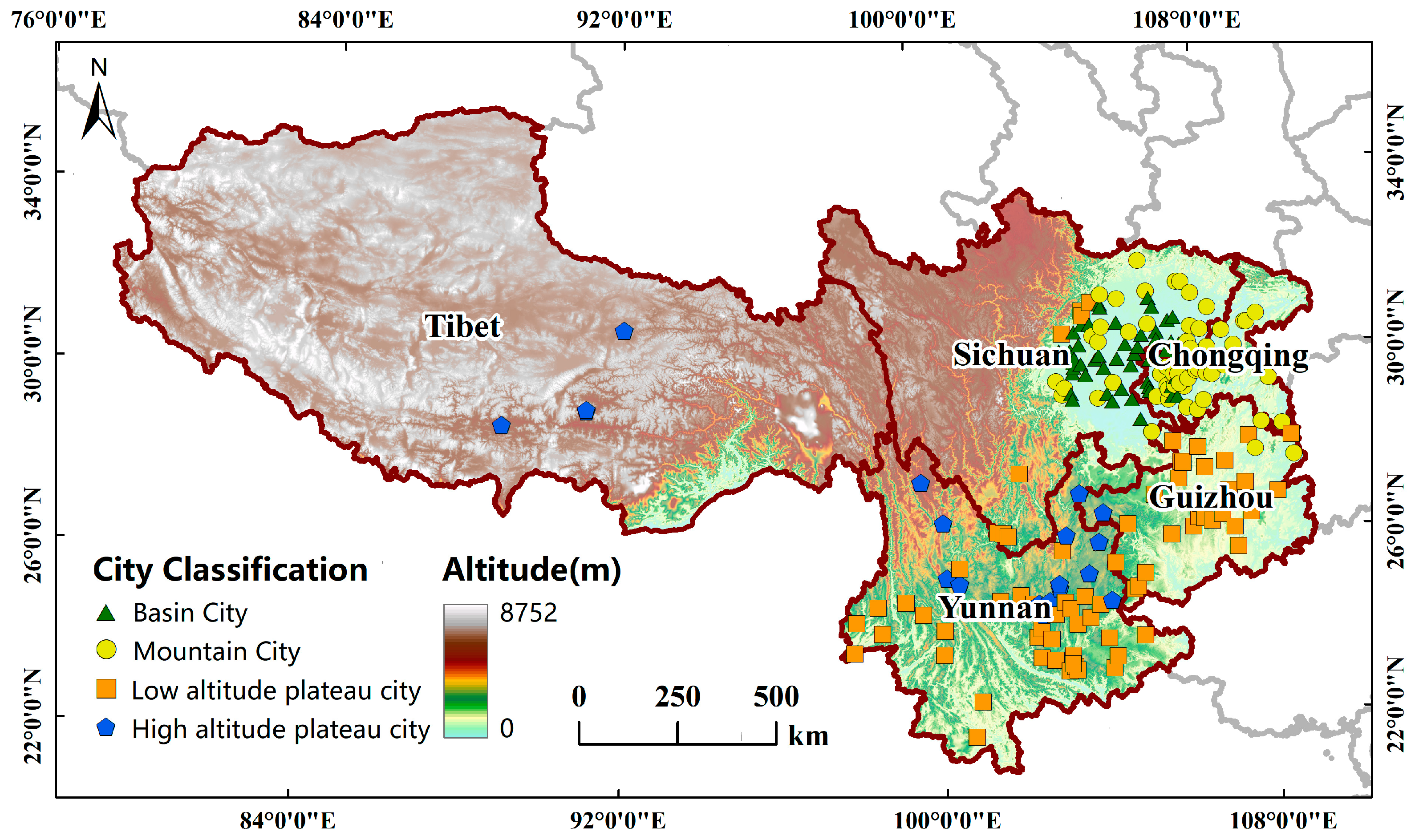
2.1. Study Area

The study area is situated in southwestern China, covering Chongqing Municipality, Sichuan Province, Guizhou Province, Yunnan Province, and the Tibet Autonomous Region. It extends between longitudes 78.25° E and 109.45° E and latitudes 21.14° N and 34.32° N, spanning an area of 2.34 million square kilometers, which accounts for approximately 24.5% of China’s total land area. This region is characterized by a complex topography and distinct climatic characteristics, making it an important area for global climate change research [41,42,43,44]. Particularly, the Sichuan–Chongqing Basin, with an average elevation of about 500 m, experiences a humid subtropical monsoon climate characterized by hot summers and concentrated rainfall. The Yunnan and Guizhou plateaus, with corresponding average elevations of approximately 2000 m and 1000 m, exhibit diverse vertical climate zones. Low-elevation areas are characterized by broadleaf and coniferous forests, while high-elevation areas are characterized by meadows, shrubs, and tundra vegetation. The central Tibet Plateau, with elevations typically exceeding 3500 m, experiences low precipitation and significant diurnal temperature variations. Additionally, it is mostly covered by meadows and shrublands.
Based on the 2018 GUB data, this study chose 200 cities in southwestern China, each with an area greater than 10 km2. To investigate the differences in SUHII across cities at varying elevations, we categorized the selected cities into four types based on elevation (Figure 1): (1) 50 basin cities in eastern Sichuan (a difference in elevation between urban and rural areas of less than 50 m and average elevation of 500 m); (2) 56 hills cities in eastern Sichuan and Chongqing (a difference in elevation greater than 50 m and an average elevation of 500 m); (3) 74 low-elevation plateau cities in the Yunnan–Guizhou Plateau (an average elevation below 2000 m); (4) 20 high-elevation plateau cities in Tibet and the Yunnan Plateau (an average elevation above 2000 m) [45].

2.2. Data

2.2.1. MODIS Data

This study employed MODIS data to determine the LST, vegetation index, surface albedo, and land cover information for 2003–2022 (Table 1). The LST data, which were used to calculate SUHII, were obtained from the Aqua/MODIS daily LST product (MYD11A1) with a spatial resolution of 1 km. This study used only Aqua/MODIS LST data, as the satellite’s overpass times (at 13:30 and 01:30 local time) are relatively close to the daily maximum and minimum air temperatures, which helps to obtain more significant SUHIIs [18]. The retrieval error of the MODIS LST product was typically within ±1.0 °C [46]. To ensure accuracy, pixels with errors exceeding 2 °C were excluded from this study. The vegetation index and albedo, both having significant impacts on SUHII, were derived from the 16-day composite enhanced vegetation index (MYD13A2) and the 16-day composite albedo product (MCD43A3), both with a spatial resolution of 1 km. The land cover product (MCD12Q1), having a spatial resolution of 0.5 km, was used to exclude pixels from water, snow, and permanent wetland, thereby minimizing their impact on SUHII estimation [16]. For calculating annual and seasonal averages, summer was defined as June to August, and winter was defined as December to February of the following year.

2.2.2. Reanalysis Data

This study employed reanalysis data (ERA5_LAND_MONTHLY) from the European Centre for Medium-Range Weather Forecasts (ECMWF) for 2003–2022. With a spatial resolution of 0.1 degree, this dataset included the monthly average temperature and total precipitation, which were used to investigate the impact of climatic factors on SUHII. ERA5 Land by the ECMWF’s ERA5 reanalysis model was used to obtain global long-term terrestrial climate data [47].

2.2.3. Auxiliary Data

Auxiliary data included GUB, digital elevation models (DEMs), and population data. The GUB was derived from the global artificial imperviousness product [27] and used to delineate urban ranges. DEMs (GTOPO30), with a spatial resolution of 30 arc seconds, were used to account for the influence of elevation on SUHII estimation. Population data (GPWv411), also having a spatial resolution of 30 arc seconds, were used to examine the effect of population density on SUHII [48].

2.3. Methods

2.3.1. Calculation of SUHII

SUHII estimation depends on the accurate definition of urban and rural areas. In this study, urban areas were considered as pixels within the urban ranges derived from the GUB data. Rural areas were defined as buffer zones outside the urban areas obtained using three methods. The first method was distance-based, establishing a buffer zone of 1.5–10 km from the urban edge [16,19,49], termed as R1 (Figure 2a). The second method was area-based, defining the rural range as the eighth buffer zone equal to the urban area, termed as R2 (Figure 2b). This approach has been shown to mitigate the impact of the UHI footprint [25,50]. The third method, also area-based, established a buffer zone twice the size of the urban area [20,22,51], termed as R3 (Figure 2c). All urban and rural areas excluded water, snow, and permanent wetland pixels to minimize their influence on SUHII estimation [16].
Given the potential influence of varying elevation on LST distribution, this study introduced three elevation conditions to assess the impact of elevation on SUHII estimation. First, rural pixels with elevation differences greater than ±50 m from the median elevation of urban pixels were excluded [11]. Second, to maintain the integrity of the rural background temperature [32], rural pixels within the top and bottom 10% of elevation extremes were removed. Third, the average elevation within the urban–rural ranges was calculated, and the LST for all urban–rural pixels was adjusted to this average elevation, applying the principle that temperature decreases by 6.5 °C per 1000 m of elevation change [52,53]. These three elevation conditions are referred to as E1, E2, and E3, respectively.
Therefore, for each city, this study employed nine different rural definitions (Table 2) to calculate the SUHII (Equation (1)). After determining the LST at the urban–rural pixel scale, the annual and seasonal average SUHII values for each city, calculated for both day (1:30 p.m.) and night (1:30 a.m.) over the period from 2003 to 2022, were also computed in addition to their regional averages [11,54]. To examine the uncertainties associated with different SUHII estimation methods, all methods were also integrated in pairs to calculate the ΔSUHIIAD (i.e., the absolute difference indicating the absolute discrepancy in the SUHII estimated by different methods). A higher ΔSUHIIAD indicates greater uncertainty in SUHII estimates due to methodological differences.
SUHII = TurbanTrural
where SUHII refers to the surface urban heat island intensity, with Turban and Trural indicating the average surface temperatures of the urban area and rural area.

2.3.2. Correlation Analysis

This study primarily analyzed the correlations of four biophysical factors, namely the vegetation index, albedo, temperature, and precipitation, and two human activity factors, namely the population and urban area, to explore the potential causes of variations in SUHII. Specifically, as the vegetation can reduce the LST via evapotranspiration, the enhanced vegetation index (EVI) was used to represent green space coverage. As urban albedo was generally low, leading to enhanced heat absorption and exacerbating the urban heat island effect, white sky albedo (WSA) was adopted as an indicator of albedo. Climate factors, which are strongly associated with the UHI effect, include temperature and precipitation as the primary climate variables. Moreover, areas with greater human activity generally generate more heat emissions. Therefore, the population and urban area were used as proxies for human activity [12,22,35,55,56]. Based on the SUHII definition (Section 2.3.1), this study computed ΔEVI and ΔWSA for all rural pixels. Since biophysical factors may vary seasonally, the seasonal averages of these factors, as well as their differences between summer and winter, were also computed. Pearson’s correlation coefficients were calculated to examine the relationship between SUHII and these factors.

3. Results

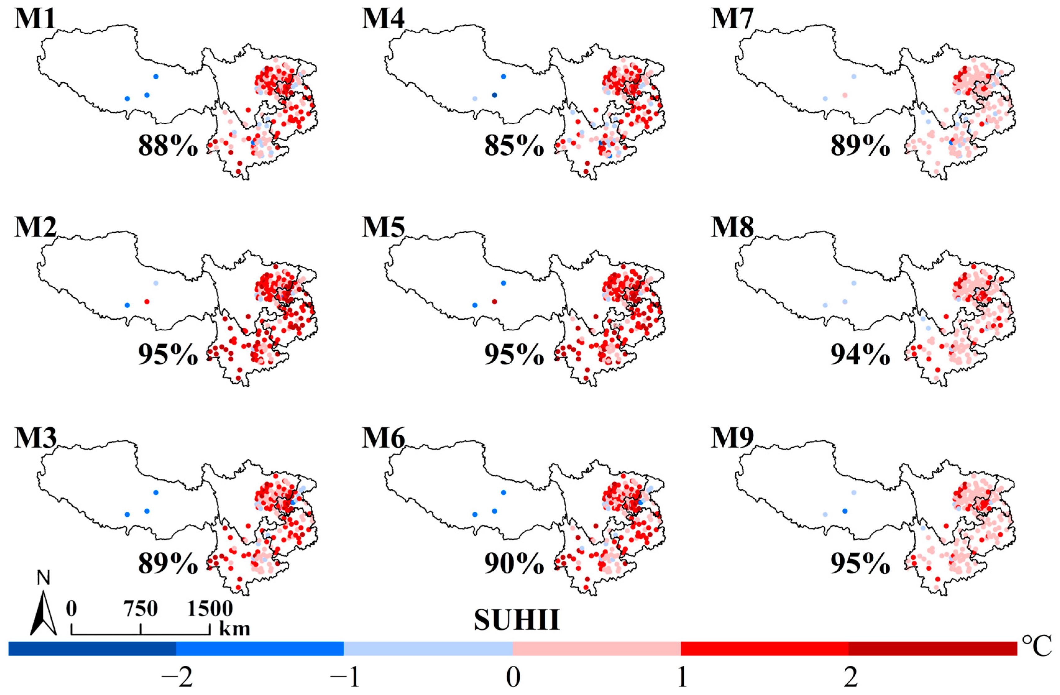
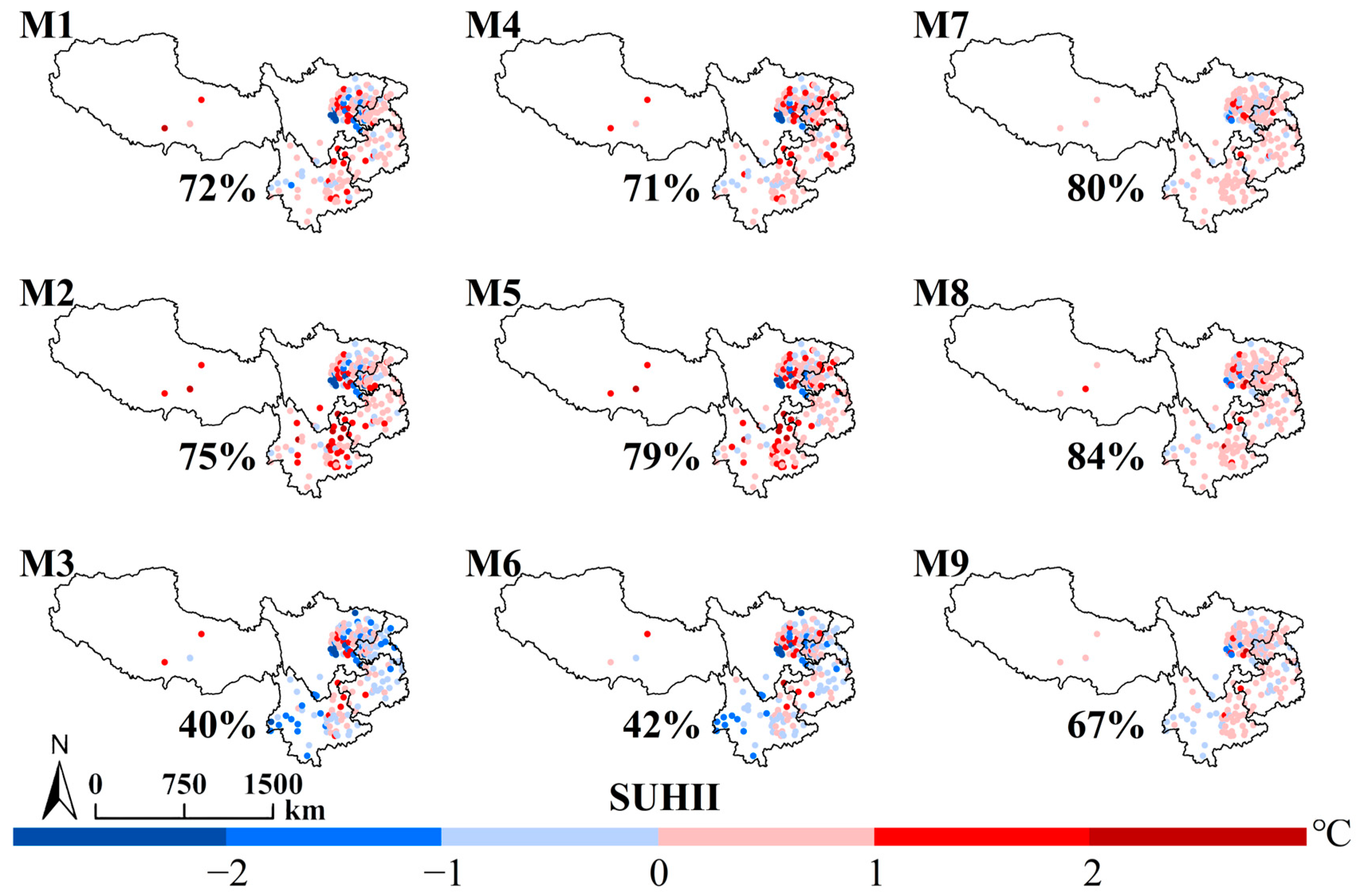
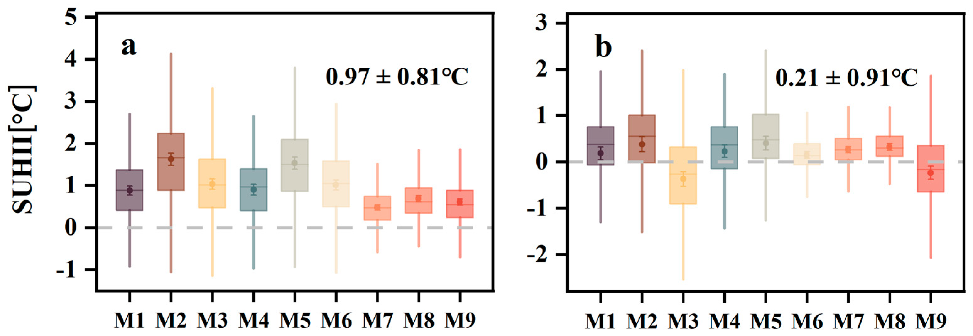
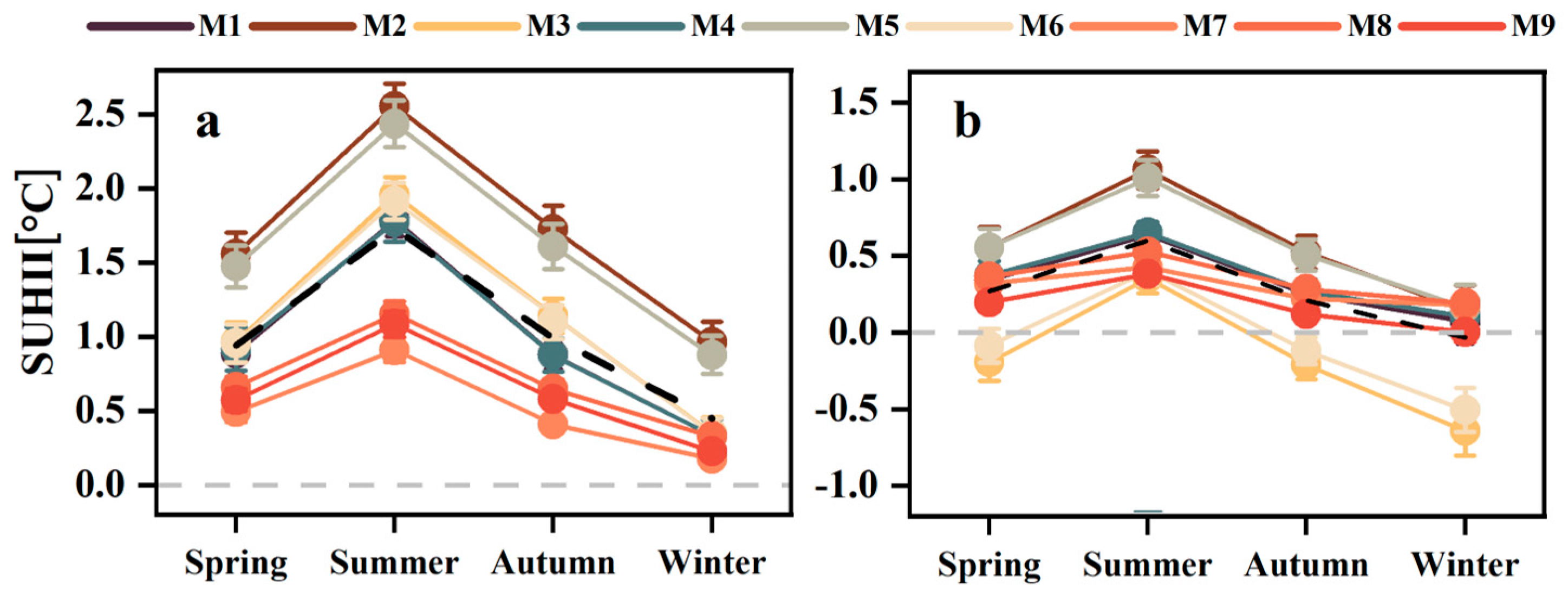
3.1. Spatiotemporal Patterns of SUHII

The results demonstrate that different methods employed for SUHII estimation influenced various characteristics of SUHII, including its thermal properties (the SUHII is considered a heat island when positive and a cool island when negative; a cool island indicates the phenomenon where urban temperatures are lower compared to the surrounding environment) [2] and its magnitude.
In terms of the magnitude of SUHII, the annual average SUHII for the selected cities (based on the mean SUHII across nine estimation methods) was 0.97 ± 0.81 °C (mean ± std) during the day and 0.21 ± 0.91 °C at night. Among the daytime SUHII values, 91% of the cities exhibited an SUHI, while 9% demonstrated an SUCI (Figure 3). At night, except for the SUHII corresponding to E3 (which adjusts the LST based on elevation differences between urban and rural areas), 77% of the cities exhibited an SUHI, and 23% demonstrated an SUCI (Figure 4). Notably, in the nighttime SUHII corresponding to E3, more than half of the cities exhibited an SUCI (Figure 4 and Figure 5). In terms of seasonal variation (Figure 6), the lowest SUHII occurred in winter (0.45 ± 0.75 °C), with spring (0.94 ± 0.92 °C) and autumn (0.99 ± 0.89 °C) being relatively close, and the highest in summer (1.73 ± 1.01 °C). A similar trend was observed at night, with an SUCI in winter (−0.03 ± 0.97 °C), the highest in summer (0.60 ± 1.65 °C), and spring (0.27 ± 0.75 °C) and autumn (0.21 ± 0.61 °C) being similar.
For the SUHII values corresponding to different methods (Figure 5), during the daytime, the maximum value was observed for M4 (1.90 ± 0.91 °C), and the minimum value for M7 (0.48 ± 0.46 °C). It was found that when the rural range was R1 and R2, the SUHII values were similar regardless of the elevation conditions. The highest SUHII values were recorded at E2 (M2: 1.62 ± 1.06 °C, M5: 1.53 ± 1.03 °C), while the lowest were at E1 (M1: 0.88 ± 0.78 °C, M4: 0.90 ± 0.91 °C). For R3, the SUHII values were generally smaller across all elevation conditions (M7: 0.48 ± 0.46 °C, M8: 0.68 ± 0.52 °C, M9: 0.60 ± 0.51 °C), with the minimum at E1 (M7: 0.48 ± 0.46 °C) and the maximum at E2 (M8: 0.68 ± 0.52 °C). Regarding seasonal variations in daytime SUHII (Figure 6), the maximum SUHII in spring was recorded for M2 (1.56 ± 1.03 °C), and the minimum for M7 (0.49 ± 0.50 °C). For the same rural range, the SUHII values were generally larger at E2 (M2: 1.56 ± 1.03 °C, M5: 1.48 ± 1.01 °C, M8: 0.66 ± 0.52 °C) and smaller at E1 (M1: 0.89 ± 0.85 °C, M4: 0.92 ± 1.06 °C, M7: 0.49 ± 0.50 °C), with E3 showing intermediate values (M3: 0.97 ± 0.95 °C, M6: 0.96 ± 0.93 °C, M9: 0.57 ± 0.53 °C). In summer, the maximum SUHII was found for M2 (2.56 ± 1.09 °C), and the minimum for M7 (0.92 ± 0.57 °C). For the same rural range, SUHII values were higher at E2 (M2: 2.56 ± 1.09 °C, M5: 2.44 ± 1.13 °C, M8: 1.15 ± 0.62 °C) and lower at E1 (M1: 1.79 ± 0.80 °C, M4: 1.78 ± 0.96 °C, M7: 0.92 ± 0.57 °C), with E3 values falling in between (M3: 1.96 ± 0.85 °C, M6: 1.91 ± 0.90 °C, M9: 1.09 ± 0.61 °C). In autumn, the maximum SUHII was observed for M2 (1.73 ± 1.15 °C), and the minimum for M7 (0.41 ± 0.35 °C). For the same rural range, SUHII values were higher at E2 (M2: 1.73 ± 1.15 °C, M5: 1.61 ± 1.10 °C, M8: 0.65 ± 0.48 °C) and lower at E1 (M1: 0.88 ± 0.69 °C, M4: 0.88 ± 0.81 °C, M7: 0.41 ± 0.35 °C), with E3 showing intermediate values (M3: 1.14 ± 0.84 °C, M6: 1.10 ± 0.82 °C, M9: 0.58 ± 0.44 °C). In winter, the maximum SUHII was recorded for M2 (0.96 ± 0.99 °C), and the minimum for M7 (0.17 ± 0.33 °C). For the same rural range, SUHII values were larger at E2 (M2: 0.96 ± 0.99 °C, M5: 0.88 ± 0.92 °C, M8: 0.33 ± 0.40 °C) and smaller at E1 (M1: 0.33 ± 0.66 °C, M4: 0.33 ± 0.79 °C, M7: 0.17 ± 0.33 °C), with E3 values being intermediate (M3: 0.35 ± 0.79 °C, M6: 0.34 ± 0.77 °C, M9: 0.23 ± 0.37 °C). From the annual and seasonal daytime SUHI results, it can be concluded that, when the rural range is fixed, the SUHII values are smallest at E1 and largest at E2. For R1 and R2, the SUHII values exhibit better consistency across different elevation conditions.
For the SUHII values corresponding to different methods during the nighttime (Figure 5), the SUHII values were generally smaller than those observed during the daytime. The maximum value was observed for M5 (0.40 ± 1.08 °C), and the minimum for M3 (−0.37 ± 1.12 °C). When the rural range was R2, the impact of elevation conditions on SUHII was relatively small, with the maximum value recorded at E2 (M5: 0.40 ± 1.08 °C) and the minimum at E3 (M6: 0.15 ± 0.49 °C). By contrast, when the rural range was R1, the SUHII values exhibited a larger variation with elevation, with the maximum recorded at E2 (M2: 0.38 ± 1.17 °C) and the minimum at E3 (M3: −0.37 ± 1.12 °C). For R3, the variation in SUHII values with elevation was slightly smaller than for R1, with the maximum value at E2 (M2: 0.32 ± 0.50 °C) and the minimum at E3 (M3: −0.23 ± 1.02 °C). Regarding seasonal variation in nighttime SUHII (Figure 6), in spring, the maximum SUHII was recorded for M2 (0.56 ± 0.95 °C) and the minimum for M3 (−0.19 ± 0.87 °C). For the same rural range, SUHII values were generally higher at E2 (M2: 0.56 ± 0.95 °C, M5: 0.55 ± 0.89 °C, M8: 0.37 ± 0.42 °C), intermediate at E1 (M1: 0.34 ± 0.68 °C, M4: 0.37 ± 0.68 °C, M7: 0.32 ± 0.38 °C), and lowest at E3 (M3: −0.19 ± 0.87 °C, M6: −0.09 ± 0.79 °C, M9: 0.20 ± 0.40 °C). In summer, the maximum SUHII was observed for M2 (1.06 ± 0.87 °C), and the minimum for M3 (0.36 ± 0.69 °C). For the same rural range, SUHII values were higher at E2 (M2: 1.06 ± 0.87 °C, M5: 1.01 ± 0.84 °C, M8: 0.53 ± 0.41 °C), intermediate at E1 (M1: 0.64 ± 0.47 °C, M4: 0.65 ± 0.51 °C, M7: 0.43 ± 0.33 °C), and lowest at E3 (M3: 0.36 ± 0.69 °C, M6: 0.40 ± 0.66 °C, M9: 0.38 ± 0.36 °C). In autumn, the maximum SUHII was recorded for M2 (0.52 ± 0.78 °C), and the minimum for M3 (−0.21 ± 0.68 °C). For the same rural range, SUHII values were larger at E2 (M2: 0.52 ± 0.78 °C, M5: 0.51 ± 0.73 °C, M8: 0.28 ± 0.32 °C), intermediate at E1 (M1: 0.25 ± 0.56 °C, M4: 0.27 ± 0.57 °C, M7: 0.22 ± 0.29 °C), and smallest at E3 (M3: −0.21 ± 0.68 °C, M6: −0.12 ± 0.63 °C, M9: 0.12 ± 0.29 °C). In winter, the maximum SUHII was observed for M8 (0.19 ± 0.45 °C), and the minimum for M3 (−0.64 ± 1.15 °C). For the same rural range, SUHII values were higher at E2 (M2: 0.14 ± 1.20 °C, M5: 0.16 ± 1.09 °C, M8: 0.19 ± 0.45 °C), intermediate at E1 (M1: 0.07 ± 1.05 °C, M4: 0.11 ± 1.01 °C, M7: 0.18 ± 0.45 °C), and lowest at E3 (M3: −0.64 ± 1.15 °C, M6: −0.51 ± 1.03 °C, M9: 0.01 ± 0.46 °C). From the annual and seasonal nighttime SUHI results, it can be concluded that, similar to the daytime results, when the rural range is fixed, the SUHII values are smallest at E3, often exhibiting a cool island effect, and largest at E2. When the rural range is R1 and R2, SUHII values show better consistency across different elevation conditions.
Spatially, the daytime SUHII is higher in the eastern region compared to the southern region (Figure 3). However, at night, the eastern area exhibits a cool island phenomenon alongside strong heat islands (Figure 4). This may be influenced by the UHI of surrounding cities [15]. The annual mean SUHII for each province (mean SUHII values corresponding to the nine estimation methods) shows that during the daytime, Guizhou (1.04 ± 0.69 °C) and Chongqing (1.04 ± 0.89 °C) had the highest values, followed by Sichuan (0.98 ± 0.75 °C) and Yunnan (0.93 ± 1.03 °C), while Tibet exhibited an SUCI (−0.62 ± 1.07 °C). During the nighttime, Tibet (0.93 ± 0.98 °C) had the highest SUHII, followed by Yunnan (0.35 ± 0.72 °C), with Guizhou (0.18 ± 0.63 °C) and Chongqing (0.15 ± 0.67 °C) showing similar values, and Sichuan having the lowest value (−0.04 ± 1.23 °C). In the Tibet Autonomous Region, four cities predominantly exhibited SUCIs at day and SUHIs at night. This phenomenon is illustrated by the distribution of their LST (Figure 7) and may be associated with the cooling effects of vegetation transpiration in arid areas [12].

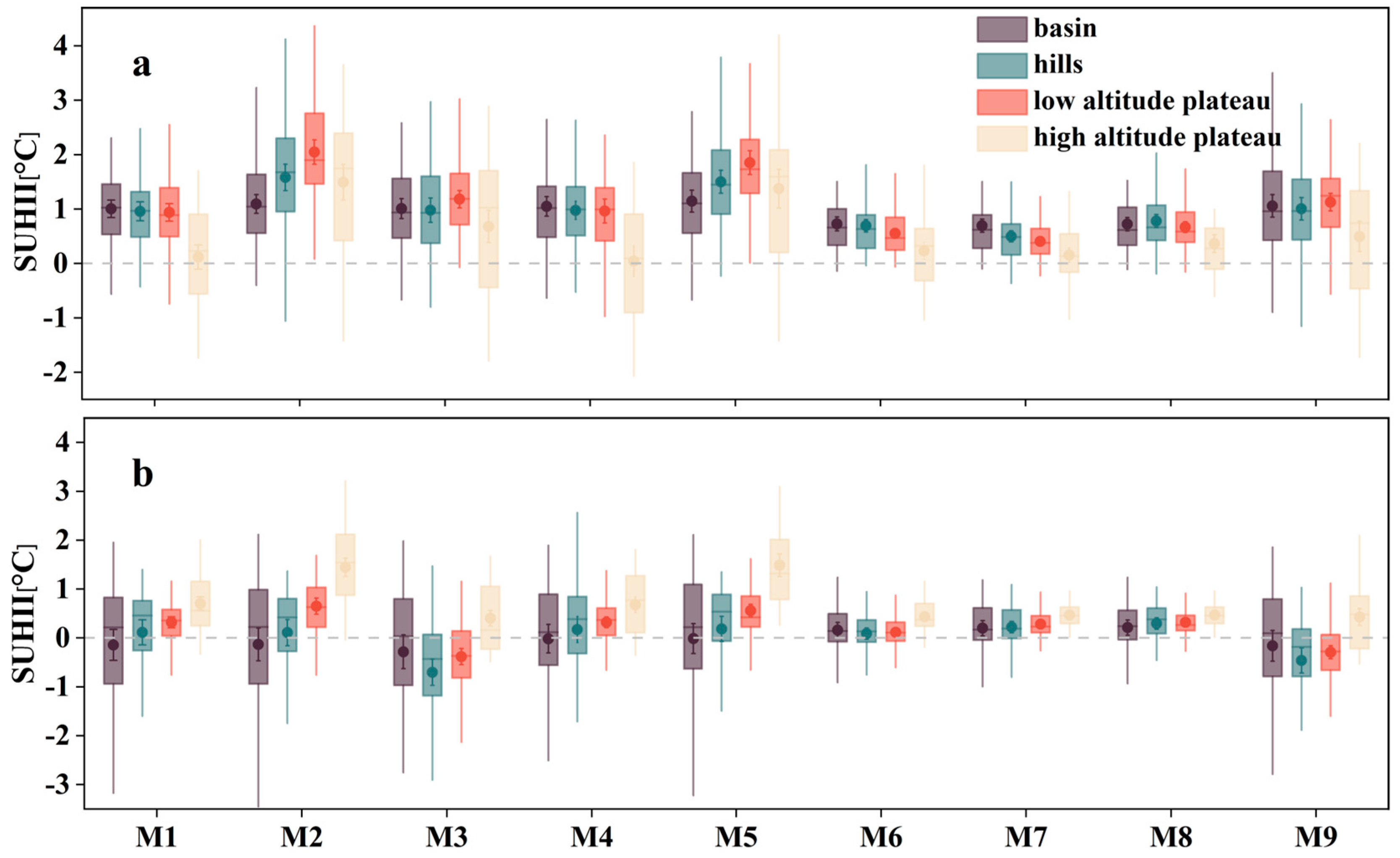
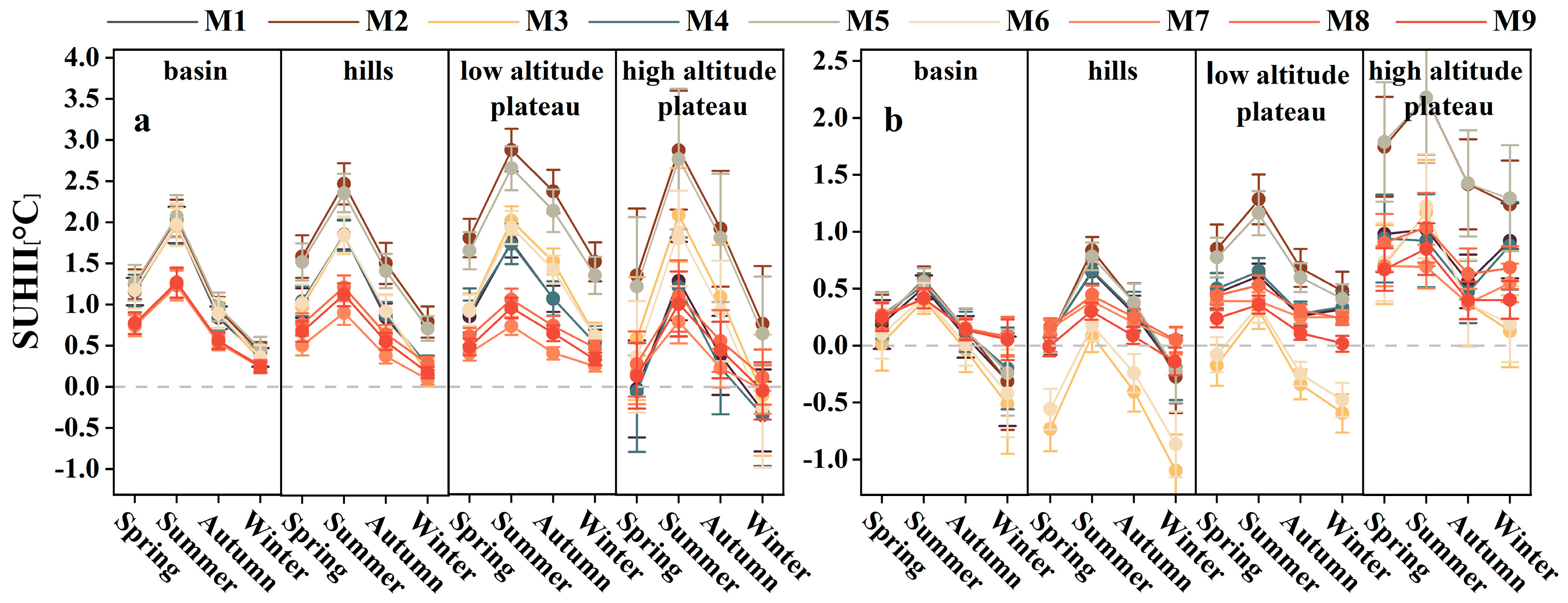
3.2. The SUHII of Four City Types

Significant regional differences in SUHII have been documented in prior research [11,12,17,57]. To examine variations in SUHII between cities, this study categorized selected cities into four elevation-based types: basin cities, hill cities, low-elevation plateau cities, and high-elevation plateau cities (Section 2.1) [45].
The results show that, for the annual average SUHII (Figure 8), during the day (Figure 8a), the SUHII values for basin cities, hill cities, and low-elevation plateau cities are generally similar across most methods, with average SUHII values of 0.95 °C, 0.99 °C, and 1.08 °C, respectively. By contrast, high-elevation plateau cities have an average SUHII of 0.55 °C, which is lower than that of the other cities by an average of 0.46 °C, except for methods M2 and M5. At night (Figure 8b), the average SUHII for basin cities, hill cities, and low-elevation plateau cities are −0.02 °C, 0 °C, and 0.21 °C, respectively. In contrast to the daytime, high-elevation plateau cities have a significantly higher average SUHII of 0.72 °C, which is 0.64 °C higher than that of the other cities. For seasonal averages SUHII (Figure 9), during the day (Figure 9a), cities in all categories show the highest SUHII in summer and the lowest in winter. The summer average SUHII for basin cities, hill cities, low-elevation plateau cities, and high-elevation plateau cities are 1.75 °C, 1.71 °C, 1.75 °C, and 1.67 °C, respectively. In winter, the average SUHII values are 0.34 °C, 0.32 °C, 0.69 °C, and 0.05 °C. High-elevation plateau cities have slightly lower SUHIIs in spring and winter compared to other regions, with values of 0.44 °C and 0.05 °C, respectively. By contrast, the spring SUHIIs for basin cities, hill cities, and low-elevation plateau cities are 1.05 °C, 1.00 °C, and 0.95 °C, respectively, and the winter SUHIIs for these cities are 0.34 °C, 0.32 °C, and 0.69 °C, which are significantly higher than those for high-elevation cities. At night (Figure 9b), the SUHII shows an increasing trend with elevation, most prominently in summer. The summer average SUHIIs for basin cities, hill cities, low-elevation plateau cities, and high-elevation plateau cities are 0.46 °C, 0.48 °C, 0.63 °C, and 1.24 °C, respectively. The summer average SUHII for high-elevation plateau cities is significantly higher than that of cities in other terrain types. Previous research on SUHIs in high-elevation areas has primarily focused on local conditions [58,59], while large-scale studies have emphasized climate zone differences [12,18,19], often overlooking elevation as a factor [13]. The present results suggest distinct diurnal SUHI patterns in high-elevation plateau cities, likely driven by their unique climatic characteristics. During the day, strong solar radiation is tempered by relatively low temperatures due to the thin atmosphere, and the high elevation results in lower atmospheric pressure, which impedes the rapid conduction or retention of heat released from the ground. As a result, heat dissipates quickly at night, leading to a higher SUHII despite the intense daytime solar radiation [60,61]. Additionally, the global SUHII study by Peng [12] found that the nighttime SUHII in Southwest China’s plateau cities exceeds the daytime SUHII, which aligns with our findings.
Finally, for the SUHII values corresponding to the nine methods, during the day, the methods with the highest SUHII values across all seasons were M2 and M5. The methods with the lowest SUHII values in basin cities, hilly cities, and low-elevation plateau cities were consistently M7, while in high-elevation plateau cities, M4 exhibited the lowest SUHII values. At night, due to varying seasonal fluctuations, there was no single method with the highest SUHII in basin and hilly cities. However, in low and high-elevation plateau cities, the highest SUHII values were consistently observed with the M2 and M5 methods. Across all seasons, the method yielding the lowest SUHII was M6.

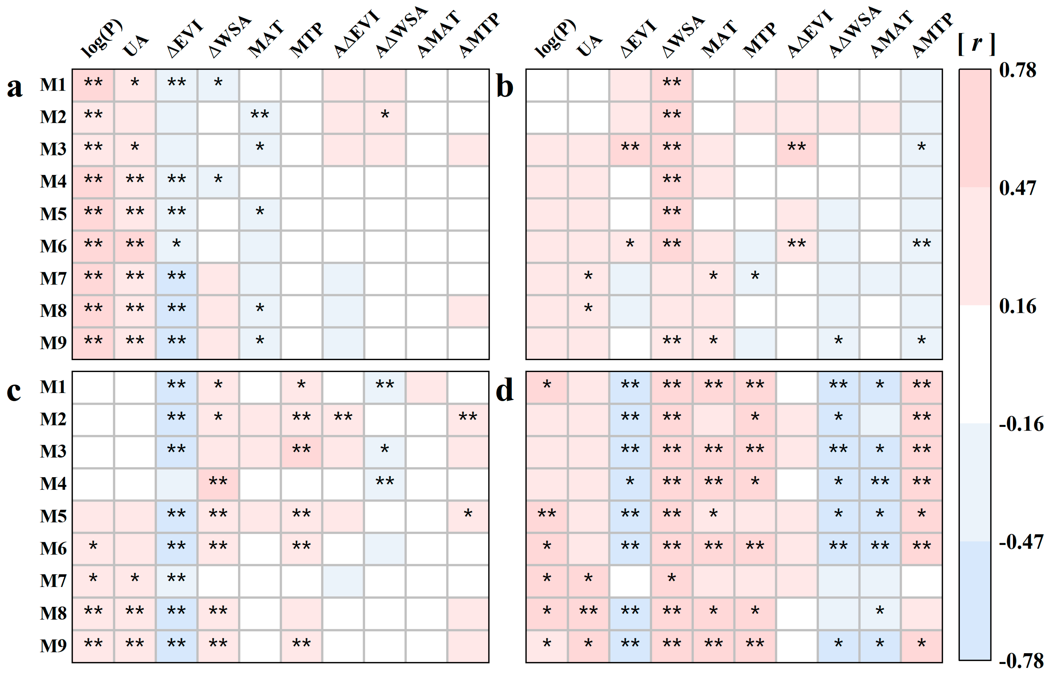
3.3. Dominant Driving Factors

3.3.1. Dominant Driving Factors of All Cities

The study also assessed the relationship between biophysical factors (ΔEVI, ΔWSA, temperature, and precipitation) and human activity factors (population and urban area) with SUHII (Figure 10, where AΔEVI, AΔWSA, AMAT, and AMTP represent the seasonal average differences of these variables between summer and winter). The results reveal variable impacts of these factors on SUHII.
In terms of ΔEVI, the daytime SUHII across all methods generally shows a negative correlation. Among them, the strongest correlations are observed between ΔEVI and SUHII for M7 (r = −0.47, p < 0.01), M8 (r = −0.62, p < 0.01), and M9 (r = −0.56, p < 0.01) when the rural range is R3. The next-strongest correlations are found for M5 (r = −0.44, p < 0.01) under the R2, but with M4 showing the weakest correlation (r = −0.24, p < 0.01), followed by M1 (r = −0.38, p < 0.01) and M2 (r = −0.38, p < 0.01) under the R1. At night, ΔEVI is negatively correlated with SUHII for M7 (r = −0.27, p < 0.01), M8 (r = −0.30, p < 0.01), and M9 (r = −0.18, p < 0.05) when the rural range is R3. For M1 to M6, ΔEVI is positively correlated with SUHII for M3 (r = 0.20, p < 0.01) and M6 (r = 0.18, p < 0.05) under E3. For the remaining methods, no significant correlation is observed. During the day, the higher correlation is attributed to the cooling effect of vegetation transpiration, which reduces urban surface temperatures [24,56]. During the night, the correlation between ΔEVI and SUHII weakens as vegetation transpiration is minimal, which is consistent with previous studies [12,62]. Regarding AΔEVI, both during the day and at night, M8 (r = −0.17, p < 0.05) and M9 (r = −0.15, p < 0.05) show a negative correlation. M2 (r = 0.25, p < 0.01), M3 (r = 0.21, p < 0.01), M5 (r = 0.18, p < 0.01), and M6 (r = 0.14, p < 0.05) exhibit positive correlations during the day, while no significant correlation is found for the other methods.
In terms of ΔWSA, a positive daytime correlation with SUHII was observed for M1 (r = 0.20, p < 0.01), M2 (r = 0.39, p < 0.01), and M3 (r = 0.28, p < 0.01) under R1, and for M7 (r = 0.21, p < 0.01), M8 (r = 0.13), and M9 (r = 0.17, p < 0.05) under R3, with the strongest correlation seen in R1. ΔWSA showed no significant correlation with SUHII for M4, M5, and M6 in R2, likely due to the lower albedo caused by urbanization, which increases solar radiation absorption in urban areas [12,63,64]. Additionally, R2 is farther from urban centers, where ΔWSA typically remains at higher levels [32]. At night, no significant correlation between ΔWSA and SUHII was found for any of the methods. Furthermore, AΔWSA showed an overall negative correlation with daytime SUHII. At night, positive correlations were observed for M1 (r = 0.22, p < 0.01) and M2 (r = 0.21, p < 0.01), while the other methods showed no significant correlation.
In terms of MAT and MTP, both showed positive correlations with SUHII during the day, although the statistical significance of these correlations varied. Regarding MAT, all methods, except for M2 (r = 0.05) and M5 (r = 0.11), demonstrated a strong positive correlation with SUHII. For the MTP, the SUHII calculated using M7 (r = −0.05), M8 (r = 0.12), and M9 (r = 0.12) under R3 did not show significant correlations with the MTP, while the remaining methods exhibited significant positive correlations. This is mainly due to the direct relationship between temperature and SUHII, whereas precipitation increases the soil moisture, which in turn lowers the LST in rural areas [6]. At night, the MAT showed a negative correlation with SUHII across all methods. Specifically, for E2, M2 (r = −0.29, p < 0.01), M5 (r = −0.28, p < 0.01), and M8 (r = −0.15, p < 0.05) exhibited a significant negative correlation with SUHII, while the remaining methods had lower significance. For the MTP, a negative correlation with SUHII was found only for M3 (r = −0.21, p < 0.01), M6 (r = −0.19, p < 0.01), and M9 (r = −0.12) under E3, with the other six methods showing no significant correlation. Seasonal variations in MAT and MTP exhibited notable differences in their relationships with SUHII for the nine methods, both during the day and at night. For example, M1 (r = 0.15, p < 0.05; r = −0.09) showed a positive correlation with AMAT but no correlation with AMTP. The specific nature of these patterns warrants further investigation.
Regarding population and urban area, both factors generally showed positive correlations with SUHII during both day and night. This relationship is likely due to higher levels of human activity and associated heat emissions in areas with greater population density and larger urban areas [13,65]. Notably, during the day, the SUHII for M2 showed no significant correlation with the population and urban area, while all other methods exhibited a significant positive correlation. Among them, M7 (r = 0.50, p < 0.01; r = 0.37, p < 0.01), M8 (r = 0.47, p < 0.01; r = 0.40, p < 0.01), and M9 (r = 0.45, p < 0.01; r = 0.37, p < 0.01) under R3 showed the strongest correlations. Compared to daytime, the correlation between SUHII and population/urban area was generally weaker at night.
In summary, when the rural range is the same, during the day, there is no clear pattern between AMAT and AMTP, while AΔEVI shows a negative correlation in R3, differing from the correlations observed in R1 and R2. Other influencing factors generally follow a consistent correlation trend. At night, AΔWSA, AMAT, and AMTP do not exhibit a clear pattern, while ΔEVI remains negatively correlated in R3, with the other factors showing generally consistent trends in terms of correlation. Overall, M7–M9 exhibit more significant correlations with various factors. When the rural range is the same, during the day, ΔEVI, urban size, population, AMAT, and AMTP show consistent correlation trends, while the other factors do not exhibit clear patterns. At night, MAT, MTP, AMAT, and AMTP follow consistent trends, whereas the remaining factors show no discernible patterns. These findings suggest that the driving mechanisms of SUHIs differ across different rural classifications, with the impact on the daytime SUHII being more significant than that at night.

3.3.2. Dominant Driving Factors of Four City Types

Factors influencing SUHII vary significantly among different city types [12,13]. This study analyzed correlations between SUHIIs in four city types (Section 2.1) and associated biophysical and human activity factors (Section 2.3.2) (Figure 11 and Figure 12). During the daytime, SUHIIs in basin cities exhibited strong correlations with the population, city size, and ΔEVI, with average Pearson coefficients of 0.54, 0.38, and −0.43, respectively. However, other factors displayed either weak or no significant correlations. In hill cities, SUHIIs correlated significantly only with ΔWSA, showing a Pearson coefficient of 0.52, with no notable associations with other variables. Low-elevation plateau cities showed strong correlations with ΔEVI, ΔWSA, and precipitation, yielding Pearson coefficients of −0.57, 0.29, and 0.32, respectively, though correlations with other factors were inconsistent. High-elevation plateau cities demonstrated significant correlations with nearly all factors, including temperature and precipitation, which were weaker or absent in other city types. This heightened sensitivity is likely due to the distinct climatic conditions of high-elevation areas [60]. At night, the correlations between SUHII and influencing factors were generally weaker across all city types [12,13,18]. Compared to the natural underlying surface around the city, SUHIs tends to elevate the urban LST, which can inhibit plant growth and photosynthesis [66], indirectly leading to changes in urban EVI values. As a result, in most cities, ΔEVI shows a negative correlation with the SUHII, while ΔWSA exhibits a positive correlation with the SUHII. Overall, basin cities remained more strongly influenced by the population and city size during the day, while high-elevation plateau cities showed greater sensitivity to both environmental and anthropogenic factors overall, underscoring their unique dynamics in SUHII [61].

4. Discussion

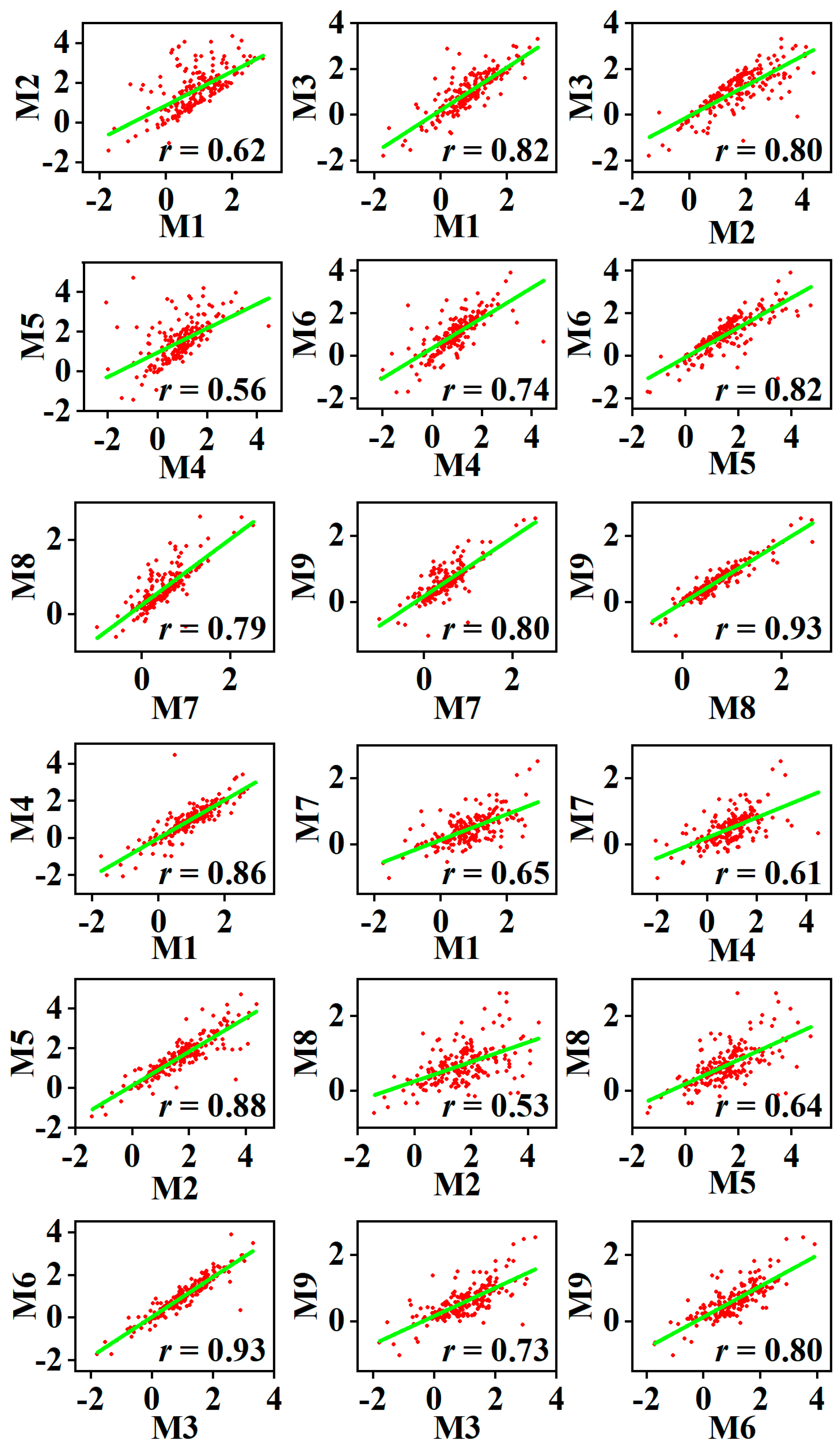
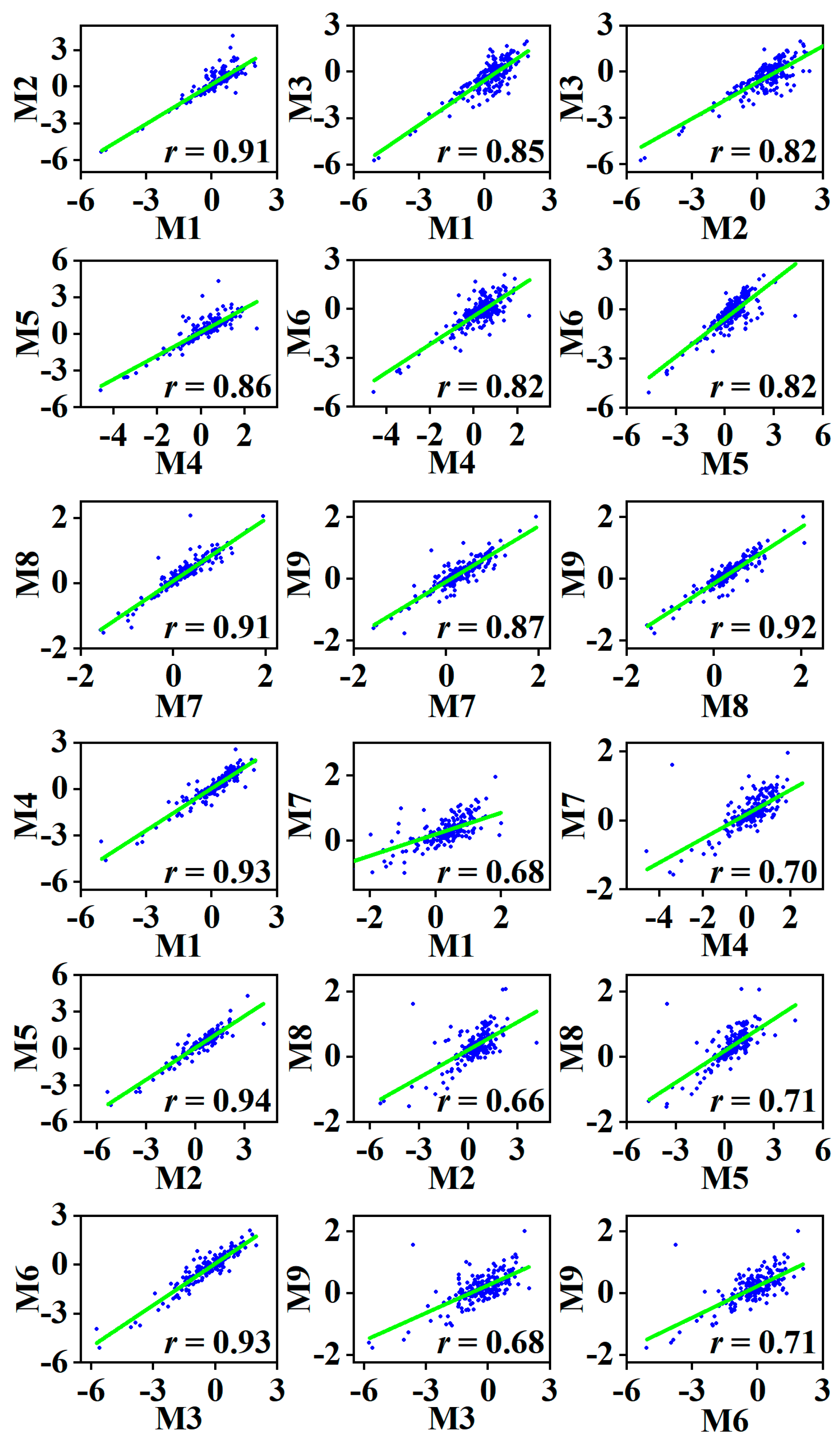
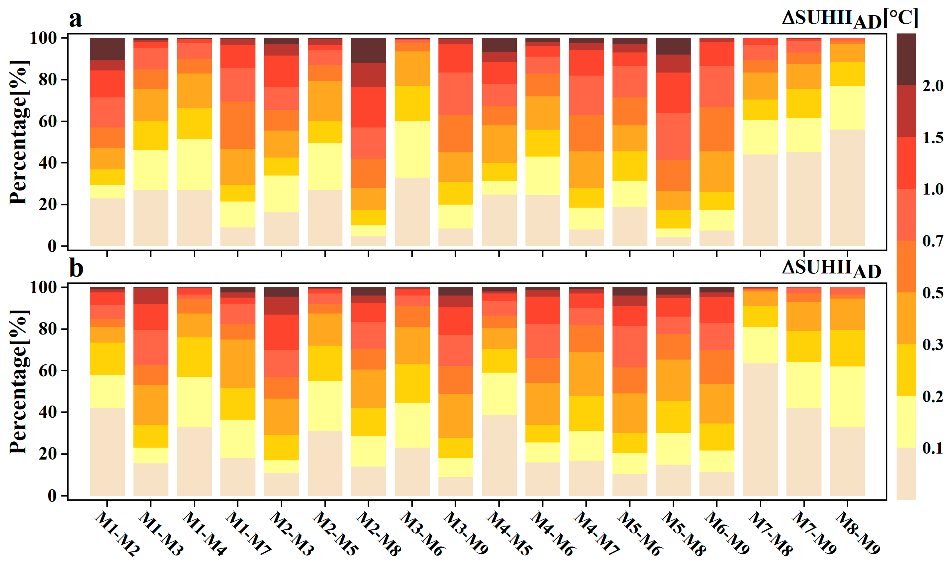
4.1. Consistency Analysis of Different Methods

Correlation analyses of SUHII using nine estimation methods indicated significant positive correlations among the methods, with variations in consistency observed (Figure 13 and Figure 14), and all results are statistically significant at the 0.01 level.
When the elevation condition is E1, the correlation of the SUHII between M1 and M4 during the day and night (r = 0.86 and r = 0.93) is higher than the correlation between M1 and M7 (r = 0.65 and r = 0.68), and between M4 and M7 (r = 0.61 and r = 0.70). The correlations at night are generally higher than those during the day. When the elevation condition is E2, the SUHII correlation between M2 and M5 is the highest during the day and night (r = 0.88 and r = 0.94), followed by M5 and M8 (r = 0.64 and r = 0.71), with the lowest correlation being between M2 and M8 (r = 0.53 and r = 0.66). Again, the correlations at night are slightly higher than those during the day. When the elevation condition is E3, the SUHII correlation between M3 and M6 is the highest during the day and night (r = 0.93 and r = 0.93), followed by M6 and M9 (r = 0.80 and r = 0.71), with the lowest being between M3 and M9 (r = 0.73 and r = 0.68). Overall, when the elevation condition is the same, R3 has a smaller impact on the SUHII calculation than R1 and R2 do.
When the rural range is R1, the minimum SUHII correlation is between M1 and M2 during the day (r = 0.62), and the maximum is between M1 and M3 (r = 0.82). At night, the maximum correlation is between M1 and M2 (r = 0.91), and the minimum is between M2 and M3 (r = 0.82). When the rural range is R2, during the day, the correlation between M4 and M5 is the smallest (r = 0.56), but at night, their correlation is the highest (r = 0.86). During the day, the maximum correlation is between M4 and M6 (r = 0.82), while at night, the correlations between M4 and M6, and M5 and M6, are the smallest (r = 0.82). When the rural range is R3, during the day, the highest correlation is between M8 and M9 (r = 0.93), with M7 and M8 (r = 0.79) and M7 and M9 (r = 0.80) showing similar correlations. At night, the correlations between M7 and M8 (r = 0.91) and M8 and M9 (r = 0.92) are similar, with the smallest correlation being between M7 and M9 (r = 0.87). Overall, when the rural range is the same, the SUHII correlation for elevation conditions E1 and E2 shows a larger difference between day and night.
A further comparison of daytime and nighttime ΔSUHIIAD, representing the absolute difference in SUHII between various estimation methods (where a larger ΔSUHIIAD indicates greater uncertainty arising from estimation methods), highlights notable patterns in southwestern cities.
During the day, the proportion of cities with a ΔSUHIIAD below 0.5 °C ranges from 26% (M5–M8) to 97% (M8–M9) (Figure 15a), with an average ΔSUHIIAD of 0.51 ± 0.01 °C calculated from the absolute differences across all methods (Figure 16a). When the rural range is R3, the ΔSUHIIAD for the M7–M8, M7–M9, and M8–M9 methods is smaller compared to R1 and R2, with the proportion of cities with a ΔSUHIIAD < 0.5 °C being 84%, 88%, and 97%, respectively. When the rural range is R1 and R2, the proportion of cities with a ΔSUHIIAD below 0.5 °C for the M1–M3 (75%) and M4–M6 (72%) methods is smaller than for other elevation conditions. When the elevation computation are the same, the proportion of cities with a ΔSUHIIAD below 0.5 °C for the M1–M4, M2–M5, and M3–M6 methods are smaller compared to other methods, with proportions of 83%, 79%, and 93%, respectively.
During the night, the proportion of cities with a ΔSUHIIAD below 0.5 °C ranges from 46% (M2–M3) to 98% (M7–M8) (Figure 15b), with an average ΔSUHIIAD of 0.44 ± 0.02 °C. The distribution pattern is similar to that of the daytime (Figure 16b). When the rural range is R3, the proportion of cities with a ΔSUHIIAD below 0.5 °C for the M7–M8 (98%), M7–M9 (93%), and M8–M9 (94%) methods is smaller compared to R1 and R2, and smaller than during the day. When the elevation computations are the same, the proportion of cities with a ΔSUHIIAD below 0.5 °C for the M1–M4 (87%), M2–M5 (87%), and M3–M6 (81%) methods is smaller compared to other methods, but the difference is smaller than during the day. Overall, the SUHII values for R1 and R2 show higher consistency, while the SUHII values for E3 exhibit smaller internal differences.

4.2. Verification of the Impact of Additional Conditions on SUHII

Previous studies on SUHIs typically controlled elevation differences between urban and rural pixels to within 50 m to minimize the impact on LST distribution [11,13,16]. By contrast, the elevation differences between urban and rural areas in the cities analyzed in this study mostly range from 100 m to 400 m, necessitating a re-evaluation of the elevation’s impact on SUHII estimation [21]. The rationale for the three supplementary conditions employed in this study is clarified as follows.
For E1, which excludes rural pixels more than ±50 m from the median urban elevation, urban and rural areas are selected at similar elevations using a fixed threshold to reduce the influence of elevation on SUHII estimation [18,22]. However, the significant elevation variations in the southwest region may lead to the exclusion of a substantial number of rural pixels, potentially affecting the accuracy of surface temperature data. The number of rural LST and land cover pixels under E1 was evaluated across different cities. In basin and hill cities, the proportion of rural pixels generally exceeds 50%, whereas in plateau cities, this proportion may fall below 10%. Furthermore, many of the excluded pixels correspond to areas dominated by grassland and forest, potentially leading to an underestimation of the SUHII [19].
For E2, which excludes rural pixels near extreme elevations, this method removes pixels at the minimum and maximum elevation values to minimize their influence on the mean LST while preserving a sufficient number of rural pixels [21]. The removal threshold was determined by analyzing the relationship between the mean rural LST and the number of rural pixels (Figure 17). A smaller proportion of rural pixels indicates a smaller elevation difference between urban and rural areas, resulting in fewer corresponding pixels. The analysis reveals that when the percentage of rural pixels is within the 90–100% range, daytime surface temperatures exhibit a more pronounced decreasing trend. Consequently, rural pixels within this elevation range were excluded.
For E3, which adjusts the LST based on elevation differences between urban and rural areas, this method corrects surface temperature distributions by accounting for mean elevation differences between these areas. Using the ELR principle that temperature decreases by 6.5 °C for every 1000 m increase in elevation, all surface temperature pixels within the urban and rural regions are adjusted according to their mean elevation [52,53]. Earlier results indicate a significant uncertainty in the corrected nighttime surface temperatures, a finding consistent with previous studies by Mentaschi [53]. Although the 6.5 °C/1000 m lapse rate in the ELR principle may be significantly influenced by local factors, it is still widely used in related studies as a reference for the relationship between air temperature and LST. This magnitude of correction remains one of the most reasonable approaches currently available for adjustment [53].

4.3. Suggestions and Limitations

In terms of practical urban construction planning, it is crucial for managers to pay closer attention to the layout of green spaces in plateau cities and strengthen measures for responding to natural disasters. Given the complex geography and specific monsoon climate in southwestern China, the rational planning of green spaces is of significant importance. Urban vegetation, especially urban forests, plays a key role in alleviating the SUHII and reducing CO2 emissions. It can effectively lower surface temperatures, improve air quality, and enhance carbon sequestration capacity. Proper green space allocation not only helps regulate the urban climate but also promotes biodiversity conservation and improves the quality of the urban ecological environment. Specifically, in plateau cities, green spaces should be prioritized in areas where the urban heat island effect is most pronounced, particularly along hillsides, valleys, and city centers. By strategically planning forest and green belts, local temperatures can be further reduced [67]. Regarding cooling strategies, policymakers should consider the specific geographical, climatic, and socio-economic conditions of the southwestern region when making decisions. For example, given the high solar radiation and large local temperature differences in plateau areas, sustainable building materials and greening technologies, such as rooftop and vertical greening, should be integrated into urban design to mitigate the urban heat island effect [12,68].
Several aspects can be improved in future work. First, this study compares the SUHIIs in Southwest China using combinations of three rural ranges and three elevation conditions. The reason for selecting these combinations is their typicality in SUHI studies, and the absence of other comparisons does not imply they are infeasible. In fact, considering more conditions is necessary to identify the most appropriate assessment method. Second, this study only addresses terrain differences from the perspective of elevation, without considering other terrain factors such as slope and aspect. Future SUHI studies in plateau regions could further explore these factors. Third, this study analyzes differences between methods based solely on the mean SUHII over a period of time, without conducting a more comprehensive analysis from perspectives such as trends. Fourth, some conditions in this study were set based on the unique geographical features of Southwest China, which helps deepen our understanding of the urban heat island effect. However, for cities in other regions or broader global studies, different factors may need to be considered.

5. Conclusions

This study analyzes the spatiotemporal patterns and influencing factors of SUHII across 200 cities in southwestern China using nine SUHII estimation methods, which integrate three rural ranges with three elevation conditions. By comparing ΔSUHIIAD, representing the absolute differences in SUHII among estimation methods, the uncertainties arising from these approaches are quantified. The main conclusions are as follows:
(1) Regarding the magnitude of SUHII, the annual average SUHII for the selected cities (mean SUHII values for nine estimation methods) (Figure 5) is 0.97 ± 0.81 °C (mean ± std) during the day and 0.21 ± 0.91 °C at night. Among these, 91% of cities are classified as heat islands during the day, while 9% are cold islands (Figure 3). At night, except for the SUHII corresponding to E3 (which adjusts the LST based on differences in elevation between urban and rural areas), 77% of cities show heat island characteristics, and 23% are cold islands (Figure 4). Notably, more than half of the cities show cold island characteristics in the night SUHII for E3. As for the seasonal variation of SUHII (Figure 6), during the day, winter exhibits the lowest SUHII (0.45 ± 0.75 °C), followed by spring (0.94 ± 0.92 °C) and autumn (0.99 ± 0.89 °C), with summer showing the highest value (1.73 ± 1.01 °C). A similar trend is observed at night.
(2) Regarding different definitions of rural areas, when the rural range is the same, the SUHII corresponding to E1 (which excludes rural pixels more than ±50 m from the median urban elevation) is the smallest in both the annual and seasonal averages during the day, while the SUHII corresponding to E2 (which excludes rural pixels near elevation extremes) is the largest. At night, the SUHII corresponding to E3 is consistently the smallest and often exhibits an SUCI, while the SUHII corresponding to E2 is the largest. Regardless of whether it is day or night, when the rural range is R1 (1.5–10 km buffer zone around the urban area) and R2 (the eighth buffer zone equal to the urban area), the SUHII values at different elevations are more consistent. The correlation results between SUHIIs indicate that the SUHII values under E1 and E2 show a significant difference during both day and night. The ΔSUHIIAD results show that during the day, the ΔSUHIIAD between E1 and E3 is the smallest, while at night, it is the largest. When elevation conditions are the same, during the day, the SUHII difference within R3 (in which the buffer zone is twice the size of the urban area) is smaller than in R1 and R2, but the SUHII consistency in R1 and R2 is higher than that in R3. At night, the correlation of the SUHII in R1 and R2 is significantly higher than during the day, and the ΔSUHIIAD in R3 is the smallest, while the ΔSUHIIAD in R1 and R2 is smaller than in R3. Additionally, for different city categories, during the day, the SUHIIs in basin cities, mountain cities, and low-altitude plateau cities are similar across most rural area definitions, with average SUHII values of 0.95 °C, 0.99 °C, and 1.08 °C, respectively. By contrast, the average SUHII of high-altitude plateau cities is 0.55 °C, which is lower than that of the other cities by 0.46 °C in most methods, except for M2 (method 2 in Table 2) and M5 (method 5 in Table 2). At night, the average SUHIIs for basin cities, mountain cities, and low-altitude plateau cities are −0.02 °C, 0 °C, and 0.21 °C, respectively. In contrast to the day, the average SUHII of high-altitude plateau cities is 0.72 °C, which is significantly higher than that of other cities (Figure 8 and Figure 9).
(3) Regarding driving factors, when the rural range is fixed, during the day, AMAT and AMTP show no obvious patterns, while AΔEVI exhibits a negative correlation when the rural area is defined as R3, differing from the correlations in R1 and R2. Other influencing factors generally show consistent correlation trends. At night, AΔWSA, AMAT, and AMTP do not exhibit clear patterns, while ΔEVI again shows a negative correlation when the rural area is R3. Other factors also show generally consistent correlation trends. Overall, M7 to M9 show more significant correlations with various factors. When elevation conditions are consistent, during the day, the ΔEVI, urban area, population, AMAT, and AMTP demonstrate consistent correlation trends, while the other factors show no clear patterns. At night, MAT, MTP, AMAT, and AMTP exhibit consistent correlations, while the remaining factors show no significant patterns. Thus, the driving mechanisms of SUHIs vary depending on the rural area delineation method, with daytime SUHII being more strongly influenced than nighttime SUHII. Moreover, in high-altitude plateau cities, the correlation between the daytime SUHII and various influencing factors is stronger than in other regions, possibly indicating that the SUHII in these areas is more sensitive to environmental and anthropogenic factors.
In summary, this study highlights that the elevation and rural range play crucial roles in influencing SUHII estimation in the southwestern region of China. These findings emphasize the need for researchers to adopt appropriate definitions of rural areas tailored to the geographical characteristics of cities to address inconsistencies in SUHII estimation methods commonly used in UHI research. This study provides valuable insights into the challenges of UHI research in plateau regions and serves as a useful reference for future investigations into urban heat island effects in diverse geographical settings.

Author Contributions

Conceptualization, Z.M. and H.F.; methodology, Z.M. and H.F.; validation, Z.M.; formal analysis, Z.M.; investigation, Z.M. and H.F.; data curation, Z.M.; writing—original draft preparation, Z.M.; writing—review and editing, H.F., J.W. and Z.C.; visualization, Z.M.; supervision, H.F.; project administration, Z.M. and H.F.; funding acquisition, Z.M. and H.F.; All authors have read and agreed to the published version of the manuscript.

Funding

This research was supported by the National Natural Science Foundation of China (Grant No. 42101322); the Yunnan Fundamental Research Projects (Grant No. 202301AT070226; 202401AT070461); the Yunnan Xingdian Talent Support Project; the Key Laboratory of Land Satellite Remote Sensing Application, the Ministry of Natural Resources of the People’s Republic of China (Grant No. KLSMNR-G202313); and the Yunnan University Scientific Research Project (Grant No. KC–23233742).

Data Availability Statement

Data are contained within the article.

Conflicts of Interest

The authors declare no conflicts of interest.

Nomenclature

AThe difference between summer and winter
DEMDigital elevation model
ELREnvironmental lapse rate
GHSLGlobal human settlement layer
GUBGlobal urban boundary
LSTLand surface temperature
MATMonthly average temperature
MTPMonthly total precipitation
SUCISurface urban cold island
SUHISurface urban heat island
SUHIISUHI intensity
UHIUrban heat island
UAUrban area
ΔEVIUrban–rural difference in vegetation coverage
ΔSUHIIADThe absolute difference indicating the absolute discrepancy in SUHII estimated by different methods
ΔWSAUrban–rural difference in albedo
log(P)Logarithm of urban population

References

  1. Aida, M.; Yaji, M. Observations of atmospheric downward radiation in the Tokyo area. Bound. Layer Meteorol. 1979, 16, 453–465. [Google Scholar] [CrossRef]
  2. Oke, T.R. The energetic basis of the urban heat island. Q. J. R. Meteorol. Soc. 1982, 108, 1–24. [Google Scholar] [CrossRef]
  3. Wohlfahrt, G.; Tomelleri, E.; Hammerle, A. The urban imprint on plant phenology. Nat. Ecol. Evol. 2019, 3, 1668–1674. [Google Scholar] [CrossRef] [PubMed]
  4. Tan, J.; Zheng, Y.; Tang, X.; Guo, C.; Li, L.; Song, G.; Zhen, X.; Yuan, D.; Kalkstein, A.J.; Li, F.; et al. The urban heat island and its impact on heat waves and human health in Shanghai. Int. J. Biometeorol. 2010, 54, 75–84. [Google Scholar] [CrossRef]
  5. Santamouris, M. Recent progress on urban overheating and heat island research. Integrated assessment of the energy, environmental, vulnerability and health impact. Synergies with the global climate change. Energy Build. 2020, 207, 109482. [Google Scholar] [CrossRef]
  6. Rizwan, A.M.; Dennis, L.C.; Chunho, L.U. A review on the generation, determination and mitigation of Urban Heat Island. J. Environ. Sci. 2008, 20, 120–128. [Google Scholar] [CrossRef]
  7. Schwarz, N.; Lautenbach, S.; Seppelt, R. Exploring indicators for quantifying surface urban heat islands of European cities with MODIS land surface temperatures. Remote Sens. Environ. 2011, 115, 3175–3186. [Google Scholar] [CrossRef]
  8. Zhou, D.; Xiao, J.; Bonafoni, S.; Berger, C.; Deilami, K.; Zhou, Y.; Frolking, S.; Yao, R.; Qiao, Z.; Sobrino, J.A. Satellite remote sensing of surface urban heat islands: Progress, challenges, and perspectives. Remote Sens. 2018, 11, 48. [Google Scholar] [CrossRef]
  9. Hu, J.; Yang, Y.; Zhou, Y.; Zhang, T.; Ma, Z.; Meng, X. Spatial patterns and temporal variations of footprint and intensity of surface urban heat island in 141 China cities. Sustain. Cities Soc. 2022, 77, 103585. [Google Scholar] [CrossRef]
  10. Streutker, D.R. Satellite-measured growth of the urban heat island of Houston, Texas. Remote Sens. Environ. 2003, 85, 282–289. [Google Scholar] [CrossRef]
  11. Imhoff, M.L.; Zhang, P.; Wolfe, R.E.; Bounoua, L. Remote sensing of the urban heat island effect across biomes in the continental USA. Remote Sens. Environ. 2010, 114, 504–513. [Google Scholar] [CrossRef]
  12. Peng, S.; Piao, S.; Ciais, P.; Friedlingstein, P.; Ottle, C.; Bréon, F.M.; Nan, H.; Zhou, L.; Myneni, R.B. Surface urban heat island across 419 global big cities. Environ. Sci. Technol. 2012, 46, 696–703. [Google Scholar] [CrossRef] [PubMed]
  13. Zhou, D.; Zhao, S.; Liu, S.; Zhang, L.; Zhu, C. Surface urban heat island in China’s 32 major cities: Spatial patterns and drivers. Remote Sens. Environ. 2014, 152, 51–61. [Google Scholar] [CrossRef]
  14. Shen, H.; Huang, L.; Zhang, L.; Wu, P.; Zeng, C. Long-term and fine-scale satellite monitoring of the urban heat island effect by the fusion of multi-temporal and multi-sensor remote sensed data: A 26-year case study of the city of Wuhan in China. Remote Sens. Environ. 2016, 172, 109–125. [Google Scholar] [CrossRef]
  15. Shastri, H.; Barik, B.; Ghosh, S.; Venkataraman, C.; Sadavarte, P. Flip flop of day-night and summer-winter surface urban heat island intensity in India. Sci. Rep. 2017, 7, 40178. [Google Scholar] [CrossRef] [PubMed]
  16. Lai, J.; Zhan, W.; Huang, F.; Voogt, J.; Bechtel, B.; Allen, M.; Peng, S.; Hong, F.; Liu, Y.; Du, P. Identification of typical diurnal patterns for clear-sky climatology of surface urban heat islands. Remote Sens. Environ. 2018, 217, 203–220. [Google Scholar] [CrossRef]
  17. Chakraborty, T.; Lee, X. A simplified urban-extent algorithm to characterize surface urban heat islands on a global scale and examine vegetation control on their spatiotemporal variability. Int. J. Appl. Earth Obs. Geoinf. 2019, 74, 269–280. [Google Scholar] [CrossRef]
  18. Du, H.; Zhan, W.; Liu, Z.; Li, J.; Li, L.; Lai, J.; Miao, S.; Huang, F.; Wang, C.; Wang, C.; et al. Simultaneous investigation of surface and canopy urban heat islands over global cities. ISPRS J. Photogramm. Remote Sens. 2021, 181, 67–83. [Google Scholar] [CrossRef]
  19. Liu, H.; He, B.; Gao, S.; Zhan, Q.; Yang, C. Influence of non-urban reference delineation on trend estimate of surface urban heat island intensity: A comparison of seven methods. Remote Sens. Environ. 2023, 296, 113735. [Google Scholar] [CrossRef]
  20. Li, K.; Chen, Y.; Wang, M.; Gong, A. Spatial-temporal variations of surface urban heat island intensity induced by different definitions of rural extents in China. Sci. Total Environ. 2019, 669, 229–247. [Google Scholar] [CrossRef] [PubMed]
  21. Cao, C.; Lee, X.; Liu, S.; Schultz, N.; Xiao, W.; Zhang, M.; Zhao, L. Urban heat islands in China enhanced by haze pollution. Nat. Commun. 2016, 7, 12509. [Google Scholar] [CrossRef] [PubMed]
  22. Venter, Z.S.; Chakraborty, T.; Lee, X. Crowdsourced air temperatures contrast satellite measures of the urban heat island and its mechanisms. Sci. Adv. 2021, 7, eabb9569. [Google Scholar] [CrossRef] [PubMed]
  23. Chakraborty, T.; Venter, Z.S.; Qian, Y.; Lee, X. Lower urban humidity moderates outdoor heat stress. Agu Adv. 2022, 3, e2022AV000729. [Google Scholar] [CrossRef]
  24. Sun, H.; Chen, Y.; Zhan, W. Comparing surface-and canopy-layer urban heat islands over Beijing using MODIS data. Int. J. Remote Sens. 2015, 36, 5448–5465. [Google Scholar] [CrossRef]
  25. Liu, H.; Huang, B.; Zhan, Q.; Gao, S.; Li, R.; Fan, Z. The influence of urban form on surface urban heat island and its planning implications: Evidence from 1288 urban clusters in China. Sustain. Cities Soc. 2021, 71, 102987. [Google Scholar] [CrossRef]
  26. Du, H.; Zhan, W.; Voogt, J.; Bechtel, B.; Chakraborty, T.C.; Liu, Z.; Hu, L.; Wang, Z.; Li, J.; Fu, P.; et al. Contrasting trends and drivers of global surface and canopy urban heat islands. Geophys. Res. Lett. 2023, 50, e2023GL104661. [Google Scholar] [CrossRef]
  27. Li, X.; Gong, P.; Zhou, Y.; Wang, J.; Bai, Y.; Chen, B.; Hu, T.; Xiao, Y.; Xu, B.; Yang, J.; et al. Mapping global urban boundaries from the global artificial impervious area (GAIA) data. Environ. Res. Lett. 2020, 15, 094044. [Google Scholar] [CrossRef]
  28. Guo, Y.; Ren, Z.; Dong, Y.; Hu, N.; Wang, C.; Zhang, P.; Jia, G.; He, X. Strengthening of surface urban heat island effect driven primarily by urban size under rapid urbanization: National evidence from China. GIScience Remote Sens. 2022, 59, 2127–2143. [Google Scholar] [CrossRef]
  29. Hawkins, T.W.; Brazel, A.J.; Stefanov, W.L.; Bigler, W.; Saffell, E.M. The role of rural variability in urban heat island determination for Phoenix, Arizona. J. Appl. Meteorol. Climatol. 2004, 43, 476–486. [Google Scholar] [CrossRef]
  30. Zhang, X.; Yan, X.; Chen, Z. Reconstructed regional mean climate with Bayesian model averaging: A case study for temperature reconstruction in the Yunnan–Guizhou Plateau, China. J. Clim. 2016, 29, 5355–5361. [Google Scholar] [CrossRef]
  31. Yang, Q.; Xu, Y.; Tong, X.; Hu, T.; Liu, Y.; Chakraborty, T.C.; Yao, R.; Xiao, C.; Chen, S.; Ma, Z. Influence of urban extent discrepancy on the estimation of surface urban heat island intensity: A global-scale assessment in 892 cities. J. Clean. Prod. 2023, 426, 139032. [Google Scholar] [CrossRef]
  32. Yao, R.; Wang, L.; Huang, X.; Gong, W.; Xia, X. Greening in rural areas increases the surface urban heat island intensity. Geophys. Res. Lett. 2019, 46, 2204–2212. [Google Scholar] [CrossRef]
  33. Ren, T.; Zhou, W.; Wang, J. Beyond intensity of urban heat island effect: A continental scale analysis on land surface temperature in major Chinese cities. Sci. Total Environ. 2021, 791, 148334. [Google Scholar] [CrossRef]
  34. Yao, R.; Wang, L.; Huang, X.; Niu, Y.; Chen, Y.; Niu, Z. The influence of different data and method on estimating the surface urban heat island intensity. Ecol. Indic. 2018, 89, 45–55. [Google Scholar] [CrossRef]
  35. Clinton, N.; Gong, P. MODIS detected surface urban heat islands and sinks: Global locations and controls. Remote Sens. Environ. 2013, 134, 294–304. [Google Scholar] [CrossRef]
  36. Kattel, D.B.; Yao, T.; Panday, P.K. Near-surface air temperature lapse rate in a humid mountainous terrain on the southern slopes of the eastern Himalayas. Theor. Appl. Climatol. 2018, 132, 1129–1141. [Google Scholar] [CrossRef]
  37. Qian, T.; Zhao, P.; Zhang, F.; Bao, X. Rainy-season precipitation over the Sichuan basin and adjacent regions in southwestern China. Mon. Weather Rev. 2015, 143, 383–394. [Google Scholar] [CrossRef]
  38. Zhong, H.; Zhou, J.; Tang, W.; Zhou, G.; Wang, Z.; Wang, W.; Meng, Y.; Ma, J. Estimation of Near-Surface Air Temperature Lapse Rate Based on MODIS Data Over the Tibetan Plateau. IEEE J. Sel. Top. Appl. Earth Obs. Remote Sens. 2023, 16, 4767–4777. [Google Scholar] [CrossRef]
  39. Ding, L.; Zhou, J.; Zhang, X.; Liu, S.; Cao, R. Downscaling of surface air temperature over the Tibetan Plateau based on DEM. Int. J. Appl. Earth Obs. Geoinf. 2018, 73, 136–147. [Google Scholar] [CrossRef]
  40. Wang, W.; Zhou, J.; Wen, X.; Long, Z.; Zhong, H.; Ma, J.; Ding, L.; Qi, D. All-weather near-surface air temperature estimation based on satellite data over the Tibetan Plateau. IEEE J. Sel. Top. Appl. Earth Obs. Remote Sens. 2022, 15, 3340–3350. [Google Scholar] [CrossRef]
  41. Wang, G.; Bai, W.; Li, N.; Hu, H. Climate changes and its impact on tundra ecosystem in Qinghai-Tibet Plateau, China. Clim. Change 2011, 106, 463–482. [Google Scholar] [CrossRef]
  42. Huang, Q.; Long, D.; Du, M.; Zeng, C.; Qiao, G.; Li, X.; Hou, A.; Hong, Y. Discharge estimation in high-mountain regions with improved methods using multisource remote sensing: A case study of the Upper Brahmaputra River. Remote Sens. Environ. 2018, 219, 115–134. [Google Scholar] [CrossRef]
  43. Yang, Q.; Huang, X.; Yang, J.; Liu, Y. The relationship between land surface temperature and artificial impervious surface fraction in 682 global cities: Spatiotemporal variations and drivers. Environ. Res. Lett. 2021, 16, 024032. [Google Scholar] [CrossRef]
  44. Ma, Y.; Zhou, J.; Liu, S.; Zhang, W.; Zhang, Y.; Xu, Z.; Song, L.; Zhao, H. Estimation of evapotranspiration using all-weather land surface temperature and variational trends with warming temperatures for the River Source Region in Southwest China. J. Hydrol. 2022, 613, 128346. [Google Scholar] [CrossRef]
  45. Li, B.Y.; Pan, B.; Cheng, W.; Han, J.; Qi, D.; Zhu, C. Research on geomorphological regionalization of China. Acta Geogr. Sin. 2013, 68, 291–306. [Google Scholar] [CrossRef]
  46. Wan, Z.; Dozier, J. A generalized split-window algorithm for retrieving land-surface temperature from space. IEEE Trans. Geosci. Remote Sens. 1996, 34, 892–905. [Google Scholar] [CrossRef]
  47. Jiao, D.; Xu, N.; Yang, F.; Xu, K. Evaluation of spatial-temporal variation performance of ERA5 precipitation data in China. Sci. Rep. 2021, 11, 17956. [Google Scholar] [CrossRef] [PubMed]
  48. Doxsey-Whitfield, E.; MacManus, K.; Adamo, S.B.; Pistolesi, L.; Squires, J.; Borkovska, O.; Baptista, S.R. Taking advantage of the improved availability of census data: A first look at the gridded population of the world, version 4. Pap. Appl. Geogr. 2015, 1, 226–234. [Google Scholar] [CrossRef]
  49. Chakraborty, T.; Hsu, A.; Manya, D.; Sheriff, G. A spatially explicit surface urban heat island database for the United States: Characterization, uncertainties, and possible applications. ISPRS J. Photogramm. Remote Sens. 2020, 168, 74–88. [Google Scholar] [CrossRef]
  50. Yao, R.; Wang, L.; Huang, X.; Niu, Z.; Liu, F.; Wang, Q. Temporal trends of surface urban heat islands and associated determinants in major Chinese cities. Sci. Total Environ. 2017, 609, 742–754. [Google Scholar] [CrossRef]
  51. Li, K.; Chen, Y.; Gao, S. Uncertainty of city-based urban heat island intensity across 1112 global cities: Background reference and cloud coverage. Remote Sens. Environ. 2022, 271, 112898. [Google Scholar] [CrossRef]
  52. Stewart, K. Atmospheric attunements. Environ. Plan. D Soc. Space 2011, 29, 445–453. [Google Scholar] [CrossRef]
  53. Mentaschi, L.; Duveiller, G.; Zulian, G.; Corbane, C.; Pesaresi, M.; Maes, J.; Stocchino, A.; Feyen, L. Global long-term mapping of surface temperature shows intensified intra-city urban heat island extremes. Glob. Environ. Change 2022, 72, 102441. [Google Scholar] [CrossRef]
  54. Tam, B.Y.; Gough, W.A.; Mohsin, T. The impact of urbanization and the urban heat island effect on day to day temperature variation. Urban Clim. 2015, 12, 1–10. [Google Scholar] [CrossRef]
  55. Zhao, L.; Lee, X.; Smith, R.B.; Oleson, K. Strong contributions of local background climate to urban heat islands. Nature 2014, 511, 216–219. [Google Scholar] [CrossRef]
  56. Manoli, G.; Fatichi, S.; Schläpfer, M.; Yu, K.; Crowther, T.W.; Meili, N.; Burlando, P.; Katul, G.G.; Bou-Zeid, E. Magnitude of urban heat islands largely explained by climate and population. Nature 2019, 573, 55–60. [Google Scholar] [CrossRef] [PubMed]
  57. Oke, T.R.; Mills, G.; Christen, A.; Voogt, J.A. Urban Climates; Cambridge University Press: Cambridge, UK, 2017. [Google Scholar] [CrossRef]
  58. Ganbat, G.; Han, J.Y.; Ryu, Y.H.; Baik, J.J. Characteristics of the urban heat island in a high-altitude metropolitan city, Ulaanbaatar, Mongolia. Asia-Pac. J. Atmos. Sci. 2013, 49, 535–541. [Google Scholar] [CrossRef]
  59. Li, G.; Zhang, X.; Mirzaei, P.A.; Zhang, J.; Zhao, Z. Urban heat island effect of a typical valley city in China: Responds to the global warming and rapid urbanization. Sustain. Cities Soc. 2018, 38, 736–745. [Google Scholar] [CrossRef]
  60. Liu, X.; Cheng, Z.; Yan, L.; Yin, Z. Elevation dependency of recent and future minimum surface air temperature trends in the Tibetan Plateau and its surroundings. Glob. Planet. Change 2009, 68, 164–174. [Google Scholar] [CrossRef]
  61. Kuang, X.; Jiao, J.J. Review on climate change on the Tibetan Plateau during the last half century. J. Geophys. Res. Atmos. 2016, 121, 3979–4007. [Google Scholar] [CrossRef]
  62. Elmes, A.; Rogan, J.; Williams, C.; Ratick, S.; Nowak, D.; Martin, D. Effects of urban tree canopy loss on land surface temperature magnitude and timing. ISPRS J. Photogramm. Remote Sens. 2017, 128, 338–353. [Google Scholar] [CrossRef]
  63. Grimmond, C.S.B. The suburban energy balance: Methodological considerations and results for a mid-latitude west coast city under winter and spring conditions. Int. J. Climatol. 1992, 12, 481–497. [Google Scholar] [CrossRef]
  64. Oke, T.R. City size and the urban heat island. Atmos. Environ. 1973, 7, 769–779. [Google Scholar] [CrossRef]
  65. Sailor, D.J. A review of methods for estimating anthropogenic heat and moisture emissions in the urban environment. Int. J. Climatol. 2011, 31, 189–199. [Google Scholar] [CrossRef]
  66. Hong, W.; Ren, Z.; Guo, Y.; Wang, C.; Cao, F.; Zhang, P.; Hong, S.; Ma, Z. Spatiotemporal changes in urban forest carbon sequestration capacity and its potential drivers in an urban agglomeration: Implications for urban CO2 emission mitigation under China’s rapid urbanization. Ecol. Indic. 2024, 159, 111601. [Google Scholar] [CrossRef]
  67. Guo, Y.; Ren, Z.; Wang, C.; Zhang, P.; Ma, Z.; Hong, S.; Hong, W.; He, X. Spatiotemporal patterns of urban forest carbon sequestration capacity: Implications for urban CO2 emission mitigation during China’s rapid urbanization. Sci. Total Environ. 2024, 912, 168781. [Google Scholar] [CrossRef]
  68. Peng, J.; Jia, J.; Liu, Y.; Li, H.; Wu, J. Seasonal contrast of the dominant factors for spatial distribution of land surface temperature in urban areas. Remote Sens. Environ. 2018, 215, 255–267. [Google Scholar] [CrossRef]
Figure 1. Study area.
Land 14 00037 g001
Figure 2. Spatial distribution of rural ranges in Kunming; (ac) correspond to rural ranges 1 (R1), 2 (R1), and 3 (R1).
Land 14 00037 g002
Figure 3. Spatial distribution of average daytime SUHII for cities in Southwest China over the last twenty years. M1–M9 correspond to the methods described in Table 2, with the black numbers below each subplot indicating the proportion of cities with SUHI.
Land 14 00037 g003
Figure 4. Spatial distribution of average nighttime SUHII for cities in Southwest China over the last twenty years. M1–M9 correspond to the methods described in Table 2, with the black numbers below each subplot indicating the proportion of cities with SUHI.
Land 14 00037 g004
Figure 5. Box plots of the average daytime (a) and nighttime (b) SUHII for cities in Southwest China over twenty years. M1–M9 correspond to the methods described in Table 2, with the black numbers indicating the average SUHII values and standard deviations (mean ± std) for the nine estimation methods. The midline of the box indicates the median, while the colored points and error bars dictate the mean values and 95% confidence intervals, respectively.
Land 14 00037 g005
Figure 6. Seasonal variations in the average daytime (a) and nighttime (b) SUHII for cities in Southwest China over the last twenty years. M1–M9 correspond to the methods described in Table 2, with the colored points indicating the mean values and the error bars indicating the 95% confidence intervals. The black dashed line indicates the average SUHII values.
Land 14 00037 g006
Figure 7. Spatial distribution of the average daytime and nighttime LST in cities of the Tibet Autonomous Region over the last twenty years, where a, b, c, and d represent the regions of Seni District in Naqu, Duilongdeqing District, Chengguan District in Lhasa, and Sangzhuzi District in Shigatse, respectively.
Land 14 00037 g007
Figure 8. Box plots of annual average daytime (a) and nighttime (b) SUHIIs for cities in Southwest China across different terrains. The box represents the interquartile range, with the line inside indicating the median. The colored points and error bars represent the mean and the 95% confidence interval, respectively.
Land 14 00037 g008
Figure 9. Seasonal variations in the annual average daytime (a) and nighttime (b) SUHIIs for cities in Southwest China across different terrains. The colored points and error bars represent the mean values and 95% confidence intervals, respectively.
Land 14 00037 g009
Figure 10. Pearson correlation coefficients (r) between annual average daytime and nighttime SUHIIs and influencing factors. Population (log(P)); urban area (UA); enhanced vegetation index (EVI); white sky albedo (WSA); monthly average temperature (MAT); monthly total precipitation (MTP); Δ represents the difference in influencing factors between urban and rural areas; A represents the difference in influencing factors between summer and winter. Asterisks (*) denote statistical significance at the 0.05 level, while double asterisks (**) denote statistical significance at the 0.01 level.
Land 14 00037 g010
Figure 11. Pearson correlation coefficients (r) between annual average daytime SUHIIs and influencing factors for cities in Southwest China across different terrains. (ad) represent basin cities, hilly and mountainous cities, low-elevation plateau cities, and high-elevation plateau cities, respectively. Population (log(P)); urban area (UA); enhanced vegetation index (EVI); white sky albedo (WSA); monthly average temperature (MAT); monthly total precipitation (MTP); Δ represents the difference between urban and rural areas; A represents the difference between summer and winter. An asterisk (*) indicates statistical significance at the 0.05 level, and two asterisks (**) indicate statistical significance at the 0.01 level.
Land 14 00037 g011
Figure 12. Pearson correlation coefficients (r) between annual average nighttime SUHIIs and influencing factors for cities in Southwest China across different terrains. (ad) represent basin cities, hilly and mountainous cities, low-elevation plateau cities, and high-elevation plateau cities, respectively. Population (log(P)); urban area (UA); enhanced vegetation index (EVI); white sky albedo (WSA); monthly average temperature (MAT); monthly total precipitation (MTP); Δ represents the difference between urban and rural areas; A represents the difference between summer and winter. An asterisk (*) indicates statistical significance at the 0.05 level, and two asterisks (**) indicate statistical significance at the 0.01 level.
Land 14 00037 g012
Figure 13. Correlations between daytime SUHII values for the nine estimation methods. M1–M9 refer to the methods outlined in Table 2, with the horizontal and vertical axes representing the daytime SUHII (°C) for each estimation method. The red points indicate the daytime SUHII for each city, and the green line represents the trend line. The value of r denotes the correlation, and all results are statistically significant at the 0.01 level.
Land 14 00037 g013
Figure 14. Correlation between nighttime SUHII values for the nine estimation methods. M1–M9 refer to the methods outlined in Table 2, with the horizontal and vertical axes representing the nighttime SUHII (°C) for each estimation method. The blue points indicate the nighttime SUHII for each city, and the green line represents the trend line. The value of r denotes the correlation, and all results are statistically significant at the 0.01 level.
Land 14 00037 g014
Figure 15. Overlay frequency distribution of the average daytime (a) and nighttime (b) ΔSUHIIAD for cities in Southwest China over twenty years. ΔSUHIIAD represents the absolute difference in SUHII between different estimation methods. The horizontal axis denotes the ΔSUHIIAD between different methods (e.g., M1–M2 represents the ΔSUHIIAD between method 1 and method 2, as shown in Table 2), and the vertical axis represents the proportion of each ΔSUHIIAD interval.
Land 14 00037 g015
Figure 16. Box plot of the average daytime (a) and nighttime (b) ΔSUHIIAD for cities in Southwest China over twenty years. ΔSUHIIAD represents the absolute difference in SUHII between different estimation methods. The horizontal axis denotes the differences between various methods (e.g., M1–M2 represents the ΔSUHIIAD between methods 1 and 2 as described in Table 2). The black dashed line, along with the accompanying numbers, represents the mean and standard deviation (mean ± std) of the ΔSUHIIAD for all method pairs. The line inside the box indicates the median, while the colored points represent the average values.
Land 14 00037 g016
Figure 17. Relationship between the average rural LST and the number of pixels for cities in Southwest China over twenty years. Panels (ac) correspond to R1, 2, and 3, respectively.
Land 14 00037 g017
Table 1. Detailed information on data.
VariableProductTemporal
Resolution
Spatial
Resolution
Data
Year
LSTMYD11A11000 mDaily2003–2022
EVIMYD13A21000 m16-day2003–2022
Land cover type AlbedoMCD12Q1
MCD43A3
500 m
1000 m
Yearly
16-day
2003–2022
2003–2022
DEMGTOPO3030 arc s--1996
Global urban
boundary
GUB--Five years2018
PopulationGPWv41130 arc sFive years2020
Temperature and precipitationERA5_LAND0.1°Monthly2003–2022
Table 2. Detailed information on each rural area delineation method.
MethodRural RangeElevation Computation
M1 (R1 and E1)1.5–10 km buffer zone around the urban area (R1).Excludes rural pixels more than ±50 m from the median urban elevation (E1).
M2 (R1 and E2)1.5–10 km buffer zone around the urban area (R1).Excludes rural pixels near elevation extremes (E2).
M3 (R1 and E3)1.5–10 km buffer zone around the urban area (R1).Adjusts the LST based on differences in elevation between urban and rural areas (E3).
M4 (R2 and E1)The eighth buffer zone equal to the urban area (R2).Excludes rural pixels more than ±50 m from the median urban elevation (E1).
M5 (R2 and E2)The eighth buffer zone equal to the urban area (R2).Excludes rural pixels near elevation extremes (E2).
M6 (R2 and E3)The eighth buffer zone equal to the urban area (R2).Adjusts the LST based on differences in elevation between urban and rural areas (E3).
M7 (R3 and E1)The buffer zone twice the size of the urban area (R3).Excludes rural pixels more than ±50 m from the median urban elevation (E1).
M8 (R3 and E2)The buffer zone twice the size of the urban area (R3).Excludes rural pixels near elevation extremes (E2).
M9 (R3 and E3)The buffer zone twice the size of the urban area (R3).Adjusts the LST based on differences in elevation between urban and rural areas (E3).
Disclaimer/Publisher’s Note: The statements, opinions and data contained in all publications are solely those of the individual author(s) and contributor(s) and not of MDPI and/or the editor(s). MDPI and/or the editor(s) disclaim responsibility for any injury to people or property resulting from any ideas, methods, instructions or products referred to in the content.

