Abstract
Urban heat islands (UHIs) are a phenomenon of temperature rising within urban areas relative to their rural counterparts. UHIs are becoming an increasingly common problem in large cities, which appear due to excessive urbanization and reductions in natural cover and vegetation. This phenomenon negatively affects the quality of life of the residents of the affected city, causing discomfort, reducing air quality, and increasing energy demand. In this study, UHIs were detected and analyzed in the city of Split, Croatia, using data from the Landsat 8 and 9 satellite missions and ground-based measurements of air and land surface temperatures, which were conducted in July, August, and September 2024. This research compares ground-based and sensor-based temperatures, and their analysis results in the proposal of a new index: the Combined Thermal Index. The main feature of this new index, which combines measured and perceived temperature, is to improve the understanding of the impact of UHIs in the city (Split), compared to existing indices. So far, LST and air temperature have not been combined, nor have they been combined with human perception of temperature, which is important in the case of UHIs because it is these people who will ultimately feel a rise in temperature.
1. Introduction
The term “urban heat island” (UHI) refers to the increase in temperature within urban areas compared to adjacent rural areas. Their main cause is overbuilding, which replaces natural cover (vegetation) with manmade materials that absorb and then release solar radiation. While excessive urbanization in recent decades has greatly benefited city dwellers and made their lives easier, it has also led to some new issues, like this phenomenon [1]. The loss of green spaces due to urbanization has significant impacts on human life, and in terms of UHIs, the loss of vegetation also reduces their positive impact on reducing high temperatures through evapotranspiration and shading. During the process of evapotranspiration and photosynthesis, a large part of net radiation is converted into energy that is divided into latent heat flows (which convert water into vapor and cool the area) and the rest into sensible heat flows (whose share in the vegetated area is significantly smaller) [2,3]. In contrast to natural soil, rock, vegetation, and water, artificial materials used in construction have distinct hydraulic, radiative, and thermal properties [4]. Their radiative characteristics and decreased albedo have a major impact on temperature rise and UHI formation [5]. Furthermore, tall buildings contribute to the issue by reducing the release of long-wave radiation stored in building structures through the formation of urban canyons [6,7]. Wind direction and speed are influenced by the configuration of urban canyons, particularly by the ratio of building height to street width and length to width. In the case of densely distributed high buildings, wind speed is reduced, less heat is convected from the surface to the air, and the influence of UHIs is increased [8,9,10]. Anthropogenic heat produced by human activities, such as traffic, electricity use, industrial processes, and human and animal biological metabolisms, also contributes to the city’s temperature [11].
UHIs can be divided into atmospheric (air) urban heat islands (AUHIs), which occur when air temperatures are higher in urban compared to rural areas, and surface urban heat islands (SUHIs), which occur when the land surface temperature (LST) in an urban area arises [12]. The types of UHI are closely related to the methods of their determination, which can be direct, indirect, or physical modeling [13,14]. Direct in situ temperature measurements using meteorological stations are the main technique for measuring AUHIs, which offer high measurement accuracy [15]. But, they have two main limitations: they are expensive and have limited coverage; and existing weather stations are often in isolated locations, are few, and are at elevations and locations that are not suitable for detecting heat islands [9,16]. Remote sensing has been successfully used in UHI studies worldwide to determine SUHIs [9]. ASTER [17], MODIS [18], Sentinel-3 SLSTR [19], OLI/TIRS [20,21,22], and Landsat TM are the most frequently used sensors. Unlike direct (point) measurements, satellite images provide data for each pixel for the entire image surface (raster), but their accuracy is lower, i.e., an estimate of soil and air temperatures is obtained. The temporal resolution of freely available satellite images is another issue, as their data are only accessible while they are passing over a specific area of the planet [13]. Daytime recordings are mostly freely available, but according to Yuan et al. [23], unlike AUHIs which are more pronounced at night, SUHIs reach higher values during the day.
Seventy percent of the world’s population lived in rural areas in 1950, and since then, rapid urbanization has been ongoing. For the first time in history, the proportion of the population living in cities surpassed that of the rural population in 2007, and today, even more people reside in cities than in rural settlements [24]. Since their share is steadily increasing and is predicted by the UN [24] to reach 68% by 2050, UHIs should be taken into account in the further spatial planning of urban expansion so that the problem does not become worse over time and so that thermal stress does not cause excessive discomfort to city dwellers. Detecting regions of areas that are especially vulnerable to heat stress should be the first step in this process. Several indices were created in order to analyze and characterize SUHIs. These include the “Environmental Criticality Index” (ECI), which is based on the distribution of LST and the availability of vegetation cover [25]; the “Temperature Criticality Value” (TCV), which is dependent on the “Index-based Built-up Index” (IBI) of built-up and air temperature; and the “Urban Thermal Field Variance Index” (UTFVI), which measures temperature variations and inhomogeneity [26].
The goal of this study is the improved detection of UHIs, during daylight hours, by remote sensing methods, supported by local in situ measurements of air temperatures by proposing a new index to define UHIs and identify regions where their effects are most pronounced. The suggested index, named the Combined Thermal Index (CTI), in contrast to the indices previously mentioned, considers both human temperature perception and measurable environmental parameters which include LST, vegetation, built-up density and wetness (through the ECI). The index was tested using data from the summer of 2024 in the Split area, Croatia, where a heat island was examined. The first part of this paper contains a detailed review of the literature; the second part describes the data and methods used in this research; and the last part presents the results and draws certain conclusions.
Literature Review
A review of previous studies is given regarding developed or modified indexes like the ECI, TCV, UTFVI, Heat Vulnerability Index (HVI), and others. A literature review is presented throughout Table 1, giving the data of each study such as the year, study location, index, methodology, and main findings to gain a transparent overview. As can be seen from the table, research on UHIs’ indices has been more frequent in past five years where studies have proposed developments or modifications of the indices.
Most of the studies dealt with the ECI as presented in Table 1. They analyzed UHIs, built-up areas, and vegetation cover based on Landsat images and LST to define the ECI. Vegetation and built-up indices like the Normalized Difference Vegetation Index (NDVI), Normalized Difference Built-up Index (NDBI), Normalized Difference Water Index (NDWI), Enhanced Vegetation Index (EVI), Ratio Vegetation Index (RVI), and Built-up Index (BU) were developed and/or used to determine ECI values in different climatic and meteorological areas. These studies mainly focused on the determination of environmentally critical areas and relationship between UHIs or LST and vegetation and built-up indices [21,25,27,28,29,30,31,32,33,34,35,36,37].
Similar was examined in other studies where relationships between land cover (LC) change and SUHIs using simple linear regression models were obtained or a strong correlation between the TCV and UTFVI by analysis and a data panel was determined. These studies investigated how LST, SUHIs, the urban heat signature (UHS) and other indices can impact on UHIs’ variability as well as the UTFVI’s measure of thermal comfort [26,38,39].
On the other hand, the Heat Risk Index (HRI) was developed in studies to determine the most vulnerable areas to extreme heat and to support any medium- and long-term measures that may be defined, using LST and population density to expose hazards and different indicators to characterize vulnerability. The Geographical Information System (GIS) and Spatial Decision Support System (SPSS) were also used for the HRI’s definition, focusing on UHIs’ impact in large cities [40,41]. Similarly to the HRI, the Urban Heat-Related Risk Index (UHRI) was determined based on spatial density, exposure, and hazard indices, taking into account a number of vulnerable groups, including children, the elderly, and foreigners [42]. The Settlement Heat Sensitivity Index (SHSI) was developed for detecting sensitive settlements in cities, comprising demographic information, urban structure type temperature, and meteorological data [43], while Urban Heat Island Intensity (UHII) [44,45] was defined to calculate the hazard of absolute maximum UHIs. Based on 13 variables related to heat vulnerability, the HVI was used to select areas that are at risk and where planting trees is the most suitable. Principal component analysis was utilized to determine weights and to reduce correlated variables to a smaller number of uncorrelated components. By summing the values of weights and component scores, the HVI was obtained [46,47]. On the other hand, the HVI, based on the spatially explicit indexes for exposure, sensitivity, and adaptive capacity, was defined using remote sensing data, principal component analysis (PCA), GIS tools, and statistical methodologies [48,49].
Several UHI risk indicators, grouped by hazard, exposure, sensitivity, and adaptive capacity, were proposed and validated by experts, residents of Bangkok, and then with confirmatory factor analysis [50], while on the other hand, several multiple vegetation and multiple land cover indices were correlated with LST [51,52].
One of the often-used thermal indices to evaluate outdoor thermal comfort and biometeorology, and one that considers a vast spectrum of thermo-physiological parameters in the heat stress analysis of UHIs, is the Universal Thermal Climate Index (UTCI) [53,54]. Provençal et al. [55] calculated the UTCI, as well as the physiological equivalent temperature (PET), humidex (HX), and wind chill index (WC), in Quebec City, Canada, where considerable seasonal climate fluctuation over a one-year period is usual. It was found that the UTCI is slightly to moderately sensitive to mean radiant temperature and humidity and very sensitive to wind speed, whereas PET is more sensitive to mean radiant temperature and can reach high values that may be hazardous more frequently than the UTCI and HX. The UTCI has a higher sensitivity to wind speed and so is more “useful” in identifying potentially hazardous weather in winter than the PET and the WC [55].
While the majority of studies on UHIs are based on various thermal indices and focus on tropical regions, many studies also examine thermal indices like the ECI and UTFVI in regions with a Mediterranean climate [40,56,57]. Both tropical and Mediterranean regions are experiencing excessive urbanization and warming, and research is required in these regions to identify and mitigate UHIs.
Furthermore, in future estimates, the Mediterranean region is regarded as one of the most prominent “hotspots” of climate change, according to [58]. Given that summers are hot and UHIs are most noticeable during this time, studies should be adjusted to the Mediterranean climate using data from the summer months.
The proposed CTI combines ECI parameters, which include the vegetation index, built-up index, and water index and temperature perception. Temperature perception was defined by interviewing habitants considering the air pressure, humidity, and wind speed that were read on the day of measurement, which were the standard conditions of a hot Split day, while the temperature was much higher than the average summer temperatures.

Table 1.
Systematic overview of literature.
Table 1.
Systematic overview of literature.
| Author(s) | Year | Location | Index | Methods and Methodology | Outcomes |
|---|---|---|---|---|---|
| Senanayake et al. [25] | 2013 | Colombo city, Sri Lanka | ECI | The spatiotemporal identification of UHIs was achieved through the analysis of thermal bands from Landsat-7 ETM+ imagery. The distribution of LST and vegetation was also examined. | To determine which parts of Colombo City were environmentally critical, a deductive index (ECI) was defined. |
| Krüger et al. [43] | 2013 | Dresden, Germany | SHSI | The study presented a methodology for detecting sensitive settlements of the city of Dresden by introducing a new SHSI. | The authors came to the conclusion that future studies should take into account the distance between thermal comfort zones and sensitive areas. |
| Umar and Kumar [27] | 2014 | Kano Metropolis, Nigeria | ECI | The various analyses involved were LST estimation, the NDVI, land use/land cover (LULC) classification, and the ECI. | The analysis indicated that the UHI intensities had a negative correlation with the NDVI and a positive correlation with built-up areas. |
| Kayet et al. [51] | 2016 | Saranda forest, Jharkhand, India | Multiple vegetation indices | Relationships between LULC, LST, and vegetation indices including the NDVI, soil-adjusted vegetation index (SAVI), RVI, and NDBI were defined using remote sensing. | The relationship between LST and the NDVI result showed a negative correlation, while there was positive relationship between LST and the NDBI. |
| Inostroza et al. [48] | 2016 | Santiago, Chile | HVI | The HVI was obtained cumulatively through the exposure, sensitivity, and adaptive capacity indices, which were calculated from several variables by statistical analysis that included PCA, a variance-weighted approach, Pearson’s correlation matrix, and Kaiser’s recommendations. | A new HVI was created that can be applied to other cities as well. |
| Ranagalage et al. [28] | 2017 | Colombo Metropolitan Area, Sri Lanka | ECI | The ECI was calculated using LST and the NDVI, while the modified NDWI (MNDWI) was used to exclude water bodies. | Through all tree time points, they found a significant correlation of LST with the NDVI (negative) and NDBI (positive). |
| Roy et al. [29] | 2017 | West Bengal, India | ECI, TFVI, land cover indices | The research analyzed the ECI and TFVI in West Bengal, India. | A negative correlation between UHI and NDVI was confirmed, and a positive correlation between the ECI and TFVI was confirmed. |
| Sharma et al. [30] | 2017 | Kolkata, West Bengal | ECI, land cover indices | The research analyzed the LULC and ECI in the area of Kolkata, West Bengal. Used indices were the NDVI, NDWI, and NDBI. | Satellite-derived biophysical variables indicated that the LST and the NDBI were increasing, while the NDVI and the NDWI were decreasing. |
| Mostofi and Hasanlou [52] | 2017 | Tehran | Multiple land cover indices | A genetic algorithm was used, kernel base one, support vector regression, and linear regression methods were used, and the relationship between LST and land cover indices was studied. | A high degree of consistency was found between affected information and the surface heat island (SHI). |
| Sasmito and Suprayogi [31] | 2018 | Surakarta City, Central Java, Indonesia | ECI | The research conducted a spatial analysis of the ECI index from Landsat images in the city of Surakarta. | The most critical environmental area was found in Surakarta City’s central region. |
| Nayak et al. [46] | 2018 | New York State | HVI | Spearman’s correlation coefficients were used to calculate correlation and principal component analysis to reduce variables to fewer components. | Urban areas with high housing density, little open space, and high percentages of the elderly, minorities, and lower-class households were the most vulnerable. |
| Werbin et al. [47] | 2019 | Boston | HVI | The HVI was used to select areas at risk, according to 13 variables, while PCA was used to assign weighting factors to each variable. | The developed tool is replicable and can be modified to other cities. |
| Krtalić et al. [21] | 2020 | Zagreb, Croatia | ECI | Two indices were calculated, the Enhanced Vegetation Index (EVI) and RVI, and a fusion of the NDVI, EVI, and RVI was made using the PCA method. Then, the ECI was calculated. | Most critical areas of Zagreb were identified. |
| Sangiorgio et al. [44] | 2020 | Multiple cities | UHII | A state-of-the-art technique was used to collect a large set of data and Analytic Hierarchy Processes (AHPs) were employed to analyze the parameters involved in the UHI phenomenon; an optimization process utilizing a Jackknife resampling technique was then employed to calibrate the index. | The study quantified the influence of 11 parameters that affect the UHII for the first time. They discovered that, with an influence of 29% and 21%, respectively, albedo and the presence of greenery represented the most significant parameters. There was a medium influence of 12%, 10%, 9%, and 8% from building height, street width, canyon orientation, and population density. The new index was developed to calculate the hazard of the absolute maximum UHII. |
| Subasinghe et al. [32] | 2021 | Colombo Distric, Sri Lanka | ECI | The NDVI, NDBI, LST, and ECI were among the spectral indices of remote sensing that were used in this study to identify aspects of environmental sustainability and urbanization in the study area. | The findings demonstrated a sharp rise in environmental criticality between 1997 and 2008, followed by a minor decline between 2008 and 2017, which corresponds with government urban planning initiatives. |
| Aprilia et al. [33] | 2021 | Surakarta City, Central Java, Indonesia | ECI | The relationship between the ECI and the UHI, LST, and the NDVI to the ECI and ECI in Surakarta were all examined in this study. | Sustainable greening is an approach to overcoming environmental criticality because green areas can mitigate the warming effects of UHIs. |
| Naim and Kafy [38] | 2021 | Chattogram, Bangladesh | UTFVI | LST and an SUHI were analyzed over 30 years using the UTFVI. The relationship between LC change and LST was examined using cross-section profiles, correlation analysis, and simple linear regression models. | The relationship between LC change and LST showed a significant positive correlation with the built-up area while it was negatively correlated with vegetation, waterbodies, and bare soil. |
| Nugraha et al. [34] | 2022 | Semarang city, Indonezija | ECI | The ECI was calculated via LST and the NDVI. The Train Random Image Classifier algorithm and supervised classification were used for land use classification. A regression analysis of the results was performed. | Through regression analysis, they found a strong relationship between the UHI and NDBI and the UHI and ECI. |
| Venturini [35] | 2022 | Santa Fe, Argentina | ECIm | The modified ECI (ECIm) was calculated using the surface temperature and vegetation index. The images of the Landsat 8 and the Google Earth Engine platform were used. | The city had a healthy thermal environment in general, except for downtown, where critical ECI values were recorded. This area was densificated with the traffic and constructions with absorbent materials. |
| Indriyani et al. [36] | 2023 | Kendari, Indonesia | ECI | After calculating the ECI using Landsat image data, LST, and the NDVI, the areas were classified into three groups based on the ECI. | The research revealed a large increase in the size of the area with a high ECI in 2021 compared to 2014 in the study area. |
| Hidalgo-García and Arco-Díaz [39] | 2022 | Granada, Spain | UTFVI | The paper investigated the spatial and temporal variability of LST, an SUHI, the UHS, and the UTFVI. And, using the Pearson correlation coefficient and data panel, it investigated the relationship between LST and the SUHI, LAST, and the NDVI, NDBI, PV, UI, and LULC and between UHS and LST, the SUHI, and the LULC. | Research demonstrated that the highest increases in LST and the SUHI were found in regions with the lowest values of the PV and NDVI, which also happened to be the regions with the highest values of the UI and NDBI. The LST had the strongest correlation with the NDBI and the weakest with PV. The UHS has a weak correlation with the LULC variable because increases in the UHS were primarily seen in the built-up and bare soil types of land covers. |
| Abrar et al. [49] | 2022 | Dhaka, Bangladesh | HVI | The HVI was determined using demographic, socioeconomic, and environmental risk variables. For the 26 normalized variables, PCA was applied for each of the 41 thanas of Dhaka for the HVI definition. | The correlation of the HVI with variables such as exposure and sensitivity was found to be highly positive, while adaptive capacity had a negative correlation with the HVI. |
| Sangiorgio et al. [45] | 2022 | Bari (Italy) | UHII | This paper calculated and analyzed UHI intensity with a multicriteria-based index, compared it to seven European cities, and proposed a different mitigation strategy to mitigate the UHII in Bari. | For the first time, useful mitigation scenarios were proposed for the city Bari. |
| Saputra and Sari [37] | 2023 | Yogyakarta, Indonesia | ECI | LST and BU indices were used to calculate the ECI, while the MNDWI was used to filter out the bodies of water. | Yogyakarta’s slums were mapped for environmental criticality in 2016 and 2021. The downtown regions were found to be in the high-criticality zone because of their high surface temperature, low vegetation, and densely populated land. |
| Lopes et al. [40] | 2023 | Porto, Portugal | HRI | A new HRI was developed, which is defined by 13 parameters in accordance with previous research. Following the indicator selection process, five experts calibrated the data and assigned weights using AHP. | The findings suggest that there is a more complex relationship than what this study could have shown between socioeconomic segregation levels and climate change vulnerability. Even in the medium and long term, reducing vulnerabilities is very challenging. Regulations that can reduce these issues should serve as the foundation for improving the HRI. |
| Putra et al. [26] | 2023 | Denpasar, Indonesia | TCV, UTFVI | The NDVI, NDBI, MNDWI, IBI, TCV, and UTFVI were calculated, and their correlation analysis was made. Taking into account the wetness factor and adjusting the surface temperature to the air temperature, the TCV index was considered an improvement over the ECI. | It was found that UTFVI and TCV had a strong correlation. The criticality was confirmed to increase with increased built-up areas and decreased vegetation. |
| Pappalardo et al. [42] | 2023 | Padua, Italy | UHRI | The UHRI is based on the presented spatial density, exposure, and hazard indices, and it takes into account a number of vulnerable groups, including children, the elderly, and foreign nationals. | In the summer of 2022, Padua had three extreme heatwaves, raising the climate risk for vulnerable social groups in six key municipal city’s sectors. |
| Thanvisitthpon [50] | 2023 | Bangkok, Thailand | Risk indicators | The research proposed a series of 46 risk indicators that were first validated by a questionnaire by experts and then by citizens, and finally a confirmatory factor analysis was performed. | A total of 46 risk indicators were grouped according to hazard, exposure, sensitivity, and adaptive capacity. |
| Elmarakby and Elkaid [41] | 2024 | Manchester, UK | HRI | The HRI was developed using remote sensing, GIS, and SPSS correlation analysis. | Approximately 30% of Manchester is affected by UHI effects, mostly areas near the city center with a higher population density and reduced green cover. |
2. Materials and Methods
In this section, the study area is described as well as data collection and data analysis, and the methodology for the new developed CTI is presented.
2.1. Study Area
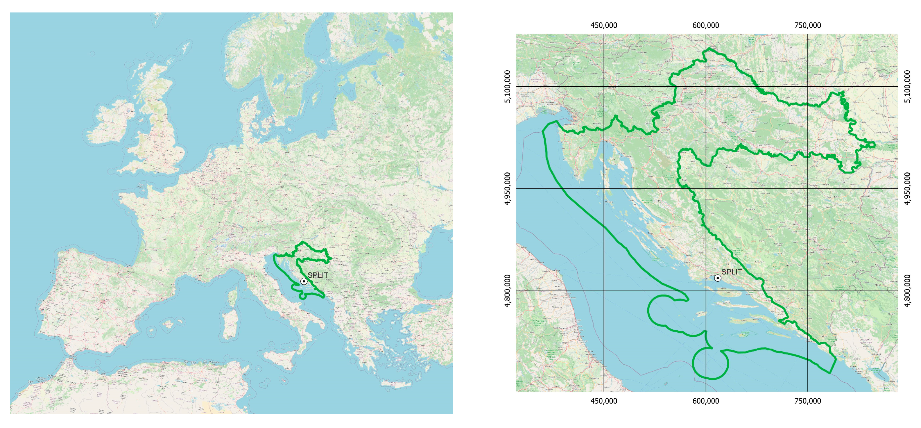
Split (43.5° N, 16.5° E) is the largest city in Dalmatia and the second largest city in the Republic of Croatia (Figure 1). It is the second-largest Croatian cargo port but also one of the leading passenger ports in the Mediterranean. It serves as the Split–Dalmatia County’s administrative center. Split is located on the Marjan peninsula on the Adriatic coast, between the Split Channel and the Gulf of Kaštela. It is surrounded by mountains, the Marjan hill that stretches across the western part of the peninsula, and the high karst mountains of the Dinaric Alps, with Mosor in the northeast and Kozjak in the northwest. By the seaside, there are the islands of Šolta, Brač, and Hvar [59,60]. According to the 2021 census, the municipality of Split has 160,577 inhabitants with a density of 2022.51 inhabitants per km2, and the urban area has 150,410 inhabitants with a density of 6495.50 inhabitants per km2 [61]. There are 27 city districts in Split, some of which were constructed without proper planning and lack greenery, which undoubtedly plays a role in the development of UHIs.
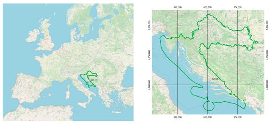
Figure 1.
The location of the study area on the map of Europe (left), and location of the city of Split in Croatia (right).
Split has a Mediterranean climate (Csa) according to the Köppen classification, which is characterized by hot, mostly dry summers and cool-to-mild, rainy winters. Although snow is extremely uncommon here, strong north winds occasionally cause days to feel colder in the Mediterranean, according to the World Atlas [59]. The average annual temperature is 16.3 °C; summertime temperatures typically range from 21.5 °C to 25.9 °C, and wintertime temperatures typically range from 7.9 °C to 10.7 °C. With an average temperature of 7.9 °C, January is the coldest month, and July is the warmest, with an average temperature of 25.9 °C [62]. The summer season spans from June to August/September, with an average of 42 hot days (average daily temperature ≥ 30 °C) during that time. The average daily temperature is calculated according to the following formula: t = (t7 + t14 + 2t21)/4, where t7, t14, and t21 are the values of the temperature measured at 7, 14, and 21 h local time, respectively. Split experiences 2640 sunny hours on average annually [63].
It is the most popular tourist destination on the Adriatic coast, so the population of the city grows dramatically during the summer. About four million passengers are served annually, which makes the Port of Split the third busiest in the Mediterranean, according to [59]. With over 3 million passengers passing through in 2023 and up to 2 million passing through between June and August of 2024, the Split airport sees high and steadily rising traffic as well [64]. Due to the rapid growth of Split’s economy, the city’s climate is also reflecting this increased activity [65].
2.2. Data Collection and Analysis
In order to account for the availability of field measurement equipment, this research was conducted during the summer of 2024, from the second half of July to mid-September. Although it might have been preferable to observe the entire summer starting in June, there were typical summer Split days during this time frame, including some that were very hot and some that were extremely hot because of the heatwave (which also occurred on 19.7). It can be said that it was the typical hot summer in Split. July and August are on average the months with the most hot days in Split when the average daily temperature is higher than 30 (July 18 days, August 17 days) and it is dry and precipitation is not common (with an average of 5 rainy days each), while June and September are somewhat colder and have more rainy days. Fakultet, Kopilica, and Bauhaus were the sites of field measurements to confirm and compare all the data used and validate the temperatures derived from processing satellite images. The measurements were carried out using the temperature kit Testo 915i [66], a thermometer with 3 temperature probes and smartphone operation. Air temperature, contact soil temperature, and soil temperature at a depth of 5 cm were measured. All probes were thermocouple type K (class 1) probes.
Landsat 8 (OLI/TIRS) satellite images for 27 July, 12 August, and 21 August as well as Landsat 9 satellite images for 19 July, 28 July, 4 August, and 13 August were used to obtain LST (Table 2). Images from other dates were supposed to be used, but bad weather forced field measurements to be discarded, or the images were later unable to be processed because of clouds.
Table 2.
Satellite images used.
Processing level 1 satellite images in UTM (Universal Transvers Mercator) projection were downloaded. For the multispectral sensor (bands B1–B7 and B9), the spatial resolution of the recordings was 30 m; for the panchromatic band B8, it was 15 m; and for the thermal sensor (bands B10 and B11), it was 100 m (Table 2). Optical bands were used to classify images, and thermal bands were used to calculate LST. Landsat satellite systems have the benefit of being completely free to download and use, but they also pass through the Split area every eight days between 9.30 and 9.45 (UTC), when UHI activity is not at its highest.
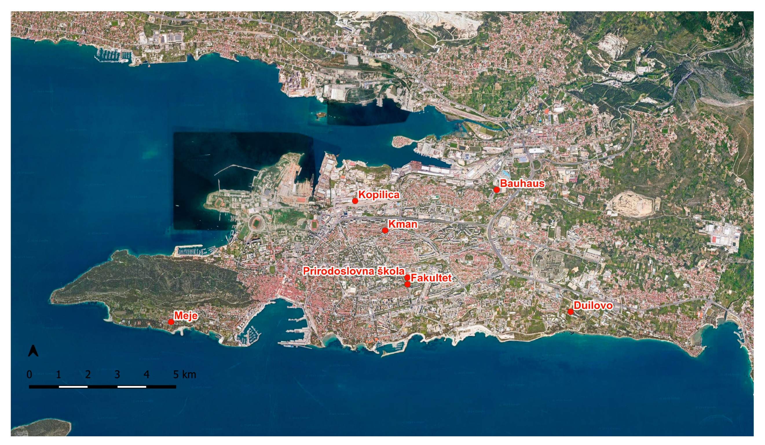
This study also planned to use official meteorological data on air and soil temperatures from the State Hydrometeorological Institute, which were measured at the Marjan meteorological station, in addition to satellite images. The meteorological station was undergoing renovations in 2024, so not all the data were available. Additionally, because the station is situated in a forested area at 122 m above sea level on the Marjan hill, the conditions surrounding it are different from those in urban areas, so the data were ultimately not considered. For this reason, data from the Pljusak Association’s network of automatic measuring stations were used [67]. Although these data are not official, they were found to be very accurate and helpful. The following stations’ data were used: Meje, Duilovo, Kman, and the School of Natural Sciences. The measuring stations and field measurement locations are shown in Figure 2.
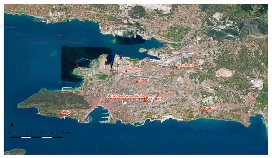
Figure 2.
The area of Split and the measuring stations and field measurement locations (red dots).
2.3. Land Surface Temperature Retrieval
Landsat images are written in quantized and calibrated scaled digital numbers (DNs), which need to be corrected before their channels are combined with others to calculate required indices and LST. According to Rajeshwari and Mani [68], LST is the temperature of the soil’s “skin” or the temperature that is felt when the hands are placed on the earth’s surface. There is no direct method of measuring the land surface temperature or radiometric temperature because the measurement of the radiation is emitted rather than the radiometric temperature, and thermometers, such as thermodynamic temperature, cannot measure it. However, satellite thermal sensors can detect reflected radiance that can be used to calculate LST [69].
To process images in absolute radiance units, 32-bit floating-point calculations are used, and the final Level 1 product results from converting these values to 16-bit integer values [65]. In the first step, it is necessary to convert these DNs into spectral radiance using scaling factors that are available in the metadata file of each satellite image [70]:
where Lλ is spectral radiance in W/(m2 srad µm), ML is the radiance multiplicative scaling factor for the band or the gain value, Qcal is the pixel value in DNs, and AL is the radiance additive scaling factor for the band or the bias value for the band.
The second step is converting spectral radiance to the effective temperature as perceived by the satellite when emissivity is assumed to be unity called the atmosphere brightness temperature [70]:
where TB is the top of the atmosphere brightness temperature in K, K1, and K2 thermal conversion constants related to the band, available in the metadata file.
Given the assumption that the emissivity for a particular class is uniform over the entire area, to calculate LST from the atmospheric brightness temperature, it is necessary to associate the appropriate class with the appropriate emissivity. In order to achieve this, the Panfushion (version 2.4) software was used to pansharpen channels 1 through 7 using the IHS method. The land cover was then classified into four classes using the Random Forest method using the Semi-Automatic Classification plugin [71] of the QGIS software (version 3.34). Several options were examined by reviewing the literature before emissivity was assigned to individual classes. Bustamante et al. [72] provided roughly average literature values which were used in this study. The emissivity values used in various studies and the values chosen for this research are displayed in Table 3.
Table 3.
Literature-derived emissivity and emissivity used.
In the next step, the brightness temperature can be corrected for emissivity, and the real LST can be obtained according to the following equation [78]:
where LST is the corrected temperature in K, λ is the wavelength of emitted radiance (depending on the band), ρ = hcK−1 (1.438 × 10⁻² mK), h = Planck’s Constant (6.626 × 10⁻³⁴ J s−1), c is the velocity of light (2.998 × 10⁸ ms−1), K is Boltzman constant (1.38 × 10⁻²³ J K−1), and ε is the surface emissivity. In the last step, the temperature is converted to degrees Celsius:
2.4. Environmental Criticality Index
According to Senanayake et al. [25], environmental criticality is directly and inversely proportional to LST and the NDVI, respectively. They proposed a deductive index, the ECI, to calculate environmental criticality in terms of LST and vegetation cover availability (represented by the Normalized Difference Vegetation Index, NDVI). To improve the clarity and contrast of the final layer and prevent an incorrect infinite in the event that the NDVI is zero, the LST and NDVI layers must first be stretched from 1 to 255 pixel values. The ECI can then be computed using the formula below [25]:
The NDVI, or Normalized Difference Vegetation Index, describes the state and presence of vegetation, and its values range from −1 to 1. Since chlorophyll has the highest absorption of these two bands of the electromagnetic spectrum, the ratio of the NIR and red band is used for the calculation [79]. The NDVI is computed using the following formula:
where NIR is the near-infrared band (B5) and RED is the red band (B4).
In order to incorporate the built intensity into the index, [51] modified the ECI. Later, Sharma et al. [30] suggested the modification that was also applied in this study and included the wetness factor in the index. The ECI was calculated according to the following formula [30]:
The NDBI is the Normalized Difference Built-up Index, which is a measure of the intensity of built-up land and is calculated as follows [30]:
where SWIR is the short-wave infrared band (B6) and NIR is the near-infrared band (B5).
The NDWI or Normalized Difference Water Index is a water or moisture status and is calculated as follows [30]:
where GREEN is the green band (B3) and NIR is the near-infrared band (B5).
2.5. Combined Thermal Index
Following the determination of each image’s LST values, an analysis of the results was conducted to choose the image with the highest values of the thermal index for additional analysis. First, areas with LST values above 40 °C were determined for each image. Since there were images taken on four dates with the same calculated area (19 July, 27 July, 28 July, 4 August), in the next step, areas with LST values above 45 °C were determined and the largest area (23.23 km2) with that temperature was measured on the image taken on 19 July. Considering the results and the measured values of that day, the image dating 19 July 2024 was selected for further analysis.
Every neighborhood where field measurements were conducted or where measuring stations were situated, including Brda, Kman, Meje, Neslanovac, Split 3, Žnjan, and Varoš, was examined. The ECI was calculated for the area of a particular neighborhood, the value of which, according to Ranagalage et al. [28], was divided into 5 classes: very low (≤0.5), low (0.5–1), moderate (1–1.5), high (1.5–2), and very high (ECI > 2). The raster of each neighborhood was then reclassified, giving each pixel a value between 1 and 5 in relation to the prior classification. For example, pixels classified as very low were given a value of 1, while pixels classified as very high were given a value of 5. After that, the average pixel value for the whole neighborhood was determined and added to the formula for the Combined Thermal Index (CTI) as ECIclass.
In order to determine the classes for perceived temperatures, a survey was conducted among the residents of Split. Residents were asked to rate the temperatures they thought were comfortable, warm, slightly warm, hot, and very hot in light of the circumstances on 19 July. On that day, the temperature was slightly higher than the average in July in the city of Split due to a heat wave, which is why it is interesting for analysis, while humidity and wind were standard. There was either no wind or it was very light, depending on the part of the city. The primary cause of the higher temperature were the anticyclonic (high-pressure) conditions over the Adriatic Sea. Because of the absence of clouds, precipitation, and substantial wind flow in such a system, heat accumulates as a result of the persistent sunshine.
The division into classes from Matzarakis and Mayer [80] was used as a starting point for the survey. Table 4 was created based on the surveys, and then the air temperatures recorded at the measurement sites or acquired from the measurement stations were categorized, giving each location a value between 1 and 5. The resulting values were entered into the formula as TP (temperature perception), and the following formula was used to determine the final index value for each quarter:
Table 4.
Air temperature classification (modified according to Matzarakis and Mayer [80]).
3. Results
Data processing was mostly carried out in the open-source program QGIS, with the help of the Panfusion program for the sharpening of the satellite images and Microsoft Excel for calculations.
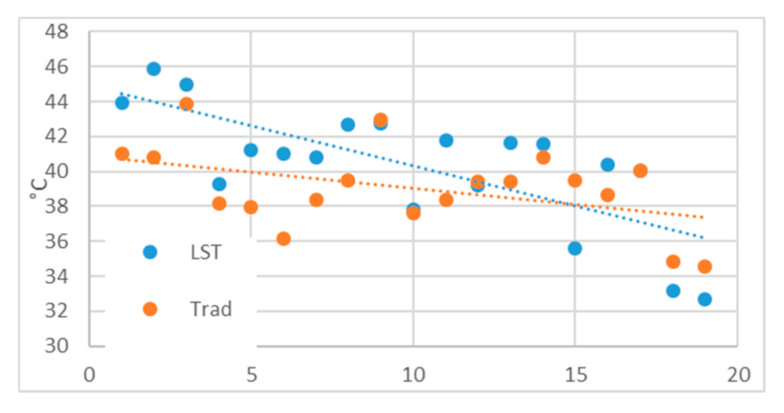
Measured ground temperatures at three measurement sites were compared with the LST derived from processing satellite images for validation purposes. The linear trend between measured temperatures and computed LST is displayed in Figure 3. Both have a negative trend, which coincides with the passage of summer and the decrease in temperature. Perhaps as a result of a greater reliance on surface properties, LST exhibits a quicker decline. With a correlation coefficient of 0.76 between the measured and computed data, it is evident that these two variables have a strong positive linear relationship and are influenced by similar factors.
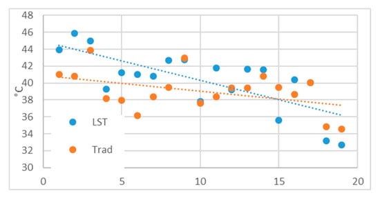
Figure 3.
Temperature trend of measured soil temperature and LST.
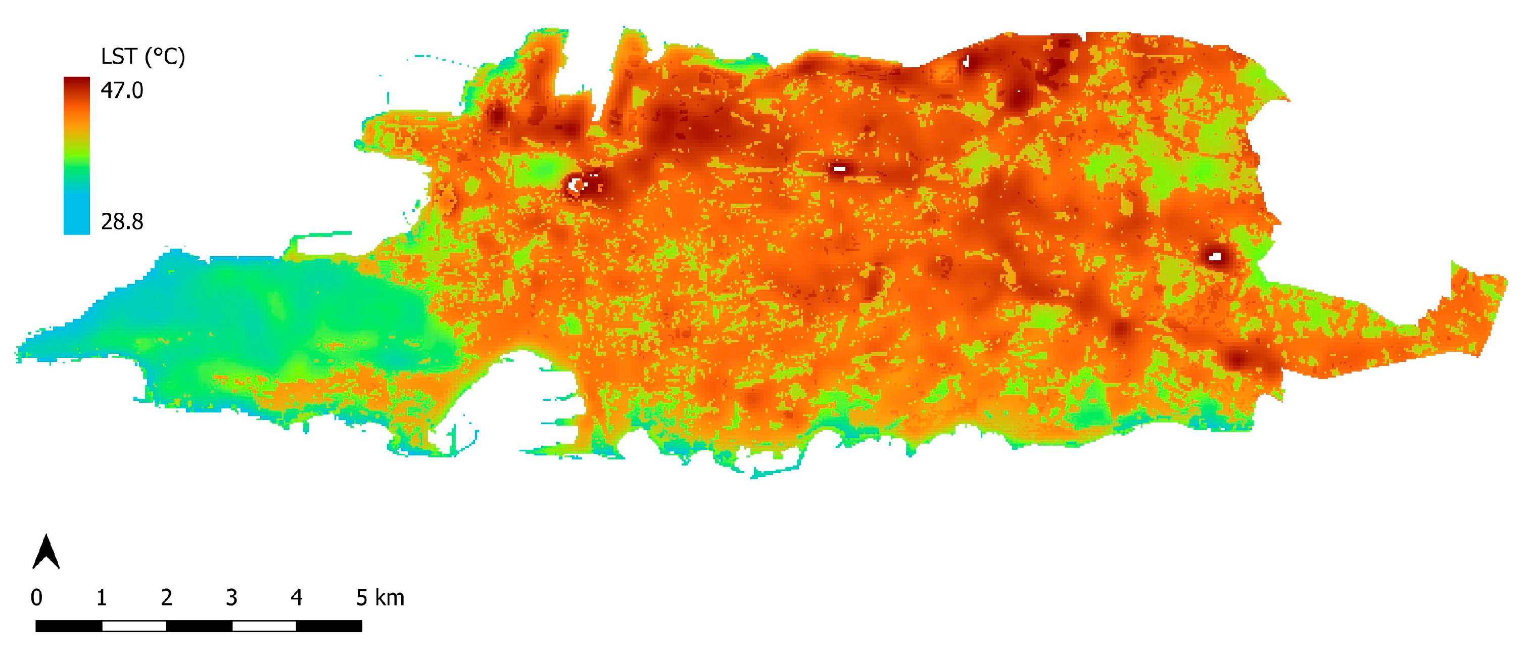
The computed LST for the Split area on the 19 July 2024, is shown in Figure 4. The west of the city has significantly lower temperatures than the rest, which is due to the presence of the Marjan forest. This makes the distinction between the urbanized and less urbanized areas of the city and the UHI phenomenon very apparent. Lower temperatures along the coast are also noticeable, which is a result of both the wind that blows from the sea to the coast and the sea’s much lower temperature, which cools the coastal area. The northern part of the city shows the highest soil temperatures, which makes sense considering that it is an industrialized part. Particularly noteworthy are the northwestern hotspot in the area where there are numerous warehouses, railways, and shipyards and the northeastern hotspot, which is a true industrial and commercial zone with large stores, paved parking lots, office buildings, and halls. It is interesting that a number of smaller hotspots, such as the campus area or the locations of individual larger shopping malls, can be noticed. These could be ascribed to both increased human activities and more concreting, particularly around shopping malls. The image also clearly shows the outlines of two major roads, Zbora narodne garde Street and Domovinskog rata street, and it would be interesting in future research to compare and study traffic and its congestion with the increase in temperature, which is undoubtedly contributed to by both the heating of the asphalt due to traffic and the exhaust gasses emitted by cars.

Figure 4.
Spatial distribution of LST in the city of Split on the 19 July 2024 (according to Landsat 9 images acquired at 9:40 UTC).
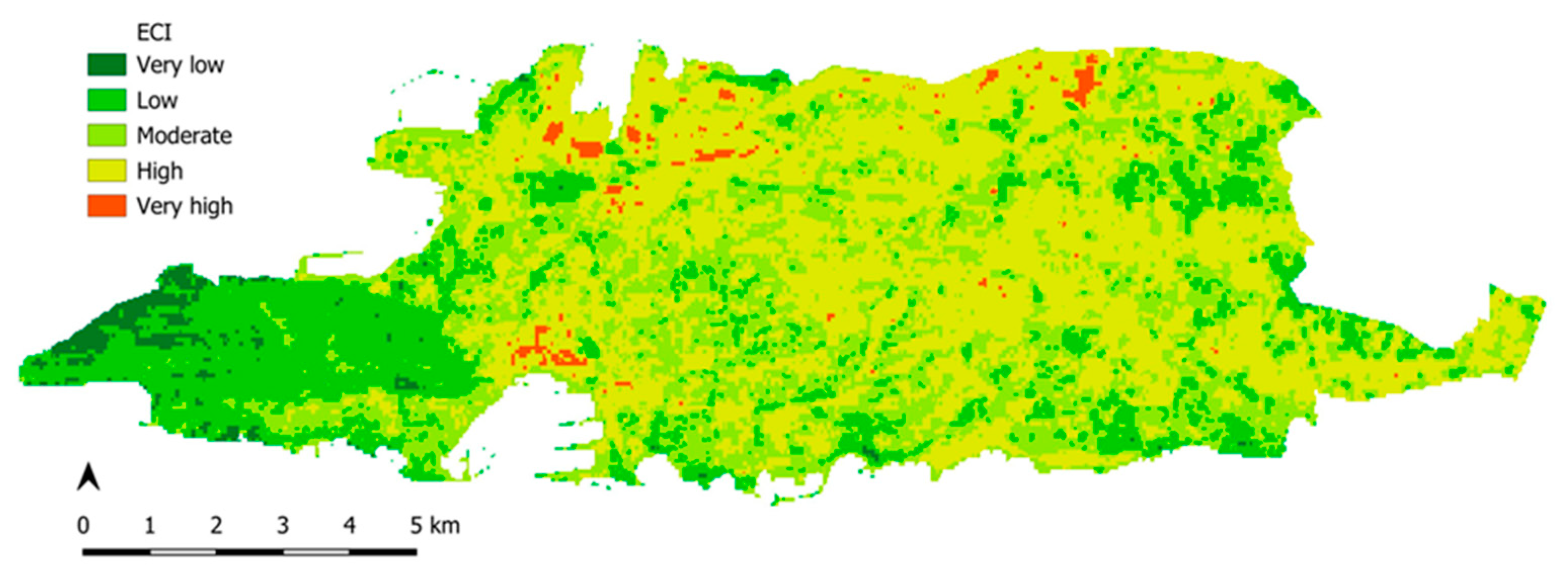
The spatial distribution with the ECI value classification is displayed in Figure 5. It is evident that the thermal hotspots depicted in Figure 4 coincide with the regions designated as very high in terms of environmental criticality. Thus, two endangered zones are visible, one in the northwest and the other in the northeast. The area that is more prominent according to this index compared to Figure 4 and soil temperature is the area of the old city core, which may be due to the very dense construction in that area, which is taken into account through the built-up index. LST and the ECI show a very high coincidence, with a correlation of 0.9.
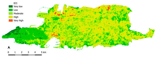
Figure 5.
The spatial distribution of the ECI in the city of Split on the 19 July 2024 (calculated from Landsat 9 images acquired at 9:40 UTC).
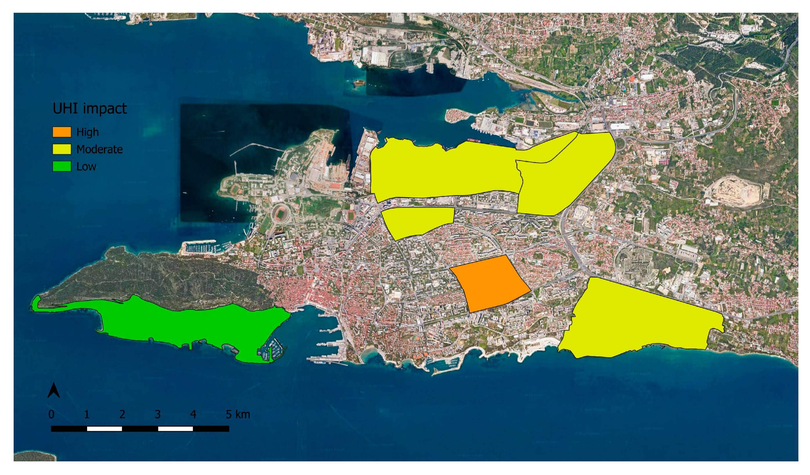
Table 5 lists the neighborhoods that were analyzed along with the corresponding measurement locations, TP, ECI class values, and, lastly, computed CTI values. In terms of UHI impact, the CTI values fall into one of the following categories: very low (1–3), low (3–5), moderate (5–7), high (7–9), and very high (9–10) UHI impact. Four neighborhoods fall into the category of moderate UHI impact, while the Meje neighborhood is categorized as having a low UHI impact (Figure 6).
Table 5.
Calculation of CTI and UHI impact.
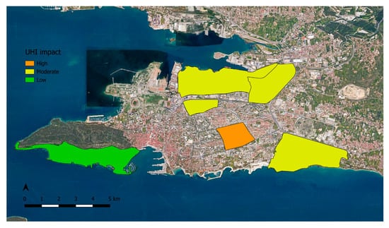
Figure 6.
UHI impact according to the CTI in parts of the city of Split on the 19 July 2024 (calculated from Landsat 9 images and field measurements acquired around 9:40 UTC).
4. Discussion
As part of this research, UHIs were detected and analyzed in the area of the city of Split, using images from the Landsat 8 and 9 satellite systems collected in the second part of the summer of 2024. A new index for monitoring the UHI phenomenon was also introduced. In addition to satellite images, field measurement data were also used, which validated the results of processing Landsat images, as well as data from measurement stations provided by the Pljusak association.
Figure 3 shows temperature trend of measured soil temperature and LST with the correlation coefficient of 0.76. The correlation may be greater, and the measurement technique may undoubtedly be one of the reasons. The measurement was not conducted at actual weather stations, and for example, minor fluctuations in the recorded temperature were noted during the wind measurement. The cause may also be the fact that point temperature measurements (although the temperatures of more materials were measured at the locations) were compared with pixel values that represent a larger surface area on which there are many materials of different emissivity.
Analyzing Figure 4 and UHI hotspots in the area of the city of Split, it can be seen that the results coincide with the results of research conducted by Duplančić Leder et al. [13] who analyzed LST in the area of the city of Split. Comparing Figure 4 and Figure 5, a high correlation can be seen, and it can be concluded that the ECI describes the heat island in the city of Split well.
The results of the calculated CTI are as expected given that the neighborhood Meje, which has a low UHI impact, is near the sea and includes a portion of the Marjan forest, which helps to cool the area. Moreover, its built-up area is not as densely built and populated as other areas of Split. Split 3 fell into the high UHI impact category since the highest air temperature was measured at that location. It should be noted that there is a micro-hotspot in that area. All obtained results also coincide with the LST and local climate zones of Split determined in the research conducted by Duplančić Leder et al. [81]. By comparing LST, the ECI, and the CTI and comparing them with previous research performed in Split [13,81], it can be said that the newly developed index provides a good representation of the UHIs in the city of Split.
5. Conclusions
Calculations of LST and the ECI revealed a strong mutual correlation, and their analysis identified UHI hotspots in the city of Split. The majority of them were found in the city’s eastern and northern regions, whereas the Marjan forest, which is situated in the far west, had low environmental criticality and LST values. The cooling effect of the sea could also be seen in the southern part of the city. These results are consistent with previous research. The results also show elevated ground temperatures that follow two major roads and smaller UHI hotspots, such as in the areas of individual shopping centers. These findings support the idea that artificial materials with low albedo are the main source of temperature increase and that this effect becomes more noticeable as the materials cover larger areas. These are also areas where greater human activity or increased car traffic is expected. Monitoring the traffic density and determining its relationship to the rising temperatures could be considered for future studies.
In order to better characterize the effects of UHI and better integrate it into future spatial planning, the study also introduced a new index known as the Combined Thermal Index, which considers human perception of temperature in addition to measurable and calculable parameters. It can be concluded that the goal of the research has been achieved and that the newly developed index, in comparison to other parameters, describes the UHIs in Split well, which, unlike the indices described so far, combines LST, built-up areas, greenery, and humidity (through the ECI index) and also takes into account air temperature and human temperature perception, which is also the crucial factor in the case of UHIs because it is these individuals who will ultimately experience an increase in temperature.
This study’s drawbacks and recommendations for future studies are as follows:
- This study included a limited number of measurement stations. To better characterize the air temperatures that were used to calculate this index and to obtain a time series, more field measurements at more locations over a longer period of time should be carried out in future studies.
- Areas that each neighborhood occupied were uneven. In future research, the study area should perhaps be divided in a different way and not by neighborhood, so that the areas are more similar (and the locations of measuring stations should also be adapted to them).
- The index should also include humidity and wind speed, as it could be applied in other non-standard conditions.
- Since people have different thermal perceptions and may not categorize the same temperatures as hot or really hot, future research could define the boundaries of the thermal perception classes in a less discrete way, for instance, by using fuzzy logic theory.
- In future research, weights could be defined so that the ECI and TP do not contribute to the final value of the UHIs’ impact in equal proportions.
Author Contributions
Conceptualization, M.Ć., K.R. and A.K.; methodology, M.Ć.; software, M.Ć.; validation, M.Ć.; formal analysis, M.Ć.; investigation, M.Ć.; resources, M.Ć.; data curation, M.Ć.; writing—original draft preparation, M.Ć.; writing—review and editing, M.Ć., K.R. and A.K.; visualization, M.Ć.; supervision, K.R. and A.K. All authors have read and agreed to the published version of the manuscript.
Funding
This research received no external funding.
Data Availability Statement
Data are contained within the article.
Acknowledgments
This research is partially supported through the project KK.01.1.1.02.0027, a project co-financed by the Croatian Government and the European Union through the European. Regional Development Fund—the Competitiveness and Cohesion Operational Programme.
Conflicts of Interest
The authors declare no conflicts of interest.
References
- Ćesić, M.; Rogulj, K.; Kilić Pamuković, J.; Krtalić, A. A Systematic Review on Fuzzy Decision Support Systems and Multi-Criteria Analysis in Urban Heat Island Management. Energies 2024, 17, 2013. [Google Scholar] [CrossRef]
- McPherson, E.G. Cooling urban heat islands with sustainable landscapes. In The Ecological City: Preserving and Restoring Urban Biodiversity; Platt, R.H., Rowntree, R.A., Muick, P.C., Eds.; University of Massachusetts Press: Amherst, MA, USA, 1994; pp. 151–172. [Google Scholar]
- Wong, N.H.; Yu, C. Study of green areas and urban heat island in a tropical city. Habitat Int. 2005, 29, 547–558. [Google Scholar] [CrossRef]
- Grimmond, S.U.E. Urbanization and global environmental change: Local effects of urban warming. Geogr. J. 2007, 173, 83–88. [Google Scholar] [CrossRef]
- USEPA. Reducing Urban Heat Islands: Compendium of Strategies—Cool Roofs. 2008. Available online: https://www.epa.gov/sites/default/files/2017-05/documents/reducing_urban_heat_islands_ch_4.pdf (accessed on 1 August 2024.).
- Taha, H. Urban climates and heat islands: Albedo, evapotranspiration, and anthropogenic heat. Energy Build. 1997, 25, 99–103. [Google Scholar] [CrossRef]
- Vitanova, L.L.; Kusaka, H. Study on the urban heat island in Sofia City: Numerical simulations with potential natural vegetation and present land use data. Sustain. Cities Soc. 2018, 40, 110–125. [Google Scholar] [CrossRef]
- Karimimoshaver, M.; Khalvandi, R.; Khalvandi, M. The effect of urban morphology on heat accumulation in urban street canyons and mitigation approach. Sustain. Cities Soc. 2021, 73, 103127. [Google Scholar] [CrossRef]
- Gartland, L.M. Heat Islands: Understanding and Mitigating Heat in Urban Areas, 1st ed.; Routledge: London, UK, 2012. [Google Scholar]
- Priyadarsini, R.; Hien, W.N.; David, C.K.W. Microclimatic modeling of the urban thermal environment of Singapore to mitigate urban heat island. Sol. Energy 2008, 82, 727–745. [Google Scholar] [CrossRef]
- Nuruzzaman, M. Urban heat island: Causes, effects and mitigation measures—A review. Int. J. Environ. Monit. Anal. 2015, 3, 67–73. [Google Scholar] [CrossRef]
- Srivanit, M.; Hokao, K. Thermal Infrared Remote Sensing for Urban Climate and Environmental Studies: Methods, Applications, and Trends. ISPRS J. Photogramm. Remote Sens. 2009, 64, 335–344. [Google Scholar] [CrossRef]
- Duplančić Leder, T.; Leder, N.; Hećimović, Ž. Split Metropolitan area surface temperature assessment with remote sensing method. Građevinar 2016, 68, 11. [Google Scholar]
- Rajasekar, U.; Weng, Q. Spatio-temporal modelling and analysis of urban heat islands by using Landsat TM and ETM+ imagery. Int. J. Remote Sens. 2009, 30, 3531–3548. [Google Scholar] [CrossRef]
- Nichol, J.E.; Fung, W.Y.; Lam, K.S.; Wong, M.S. Urban heat island diagnosis using ASTER satellite images and ‘in situ’ air temperature. Atmos. Res. 2009, 94, 276–284. [Google Scholar] [CrossRef]
- Fadhil, M.; Hamoodi, M.N.; Ziboon, A.R.T. Mitigating urban heat island effects in urban environments: Strategies and tools. In IOP Conference Series: Earth and Environmental Science; IOP Publishing: Bristol, UK, 2023; Volume 1129, p. 012025. [Google Scholar]
- Nath, B.; Ni-Meister, W.; Özdoğan, M. Fine-scale urban heat patterns in New York city measured by ASTER satellite—The role of complex spatial structures. Remote Sens. 2021, 13, 3797. [Google Scholar] [CrossRef]
- Monteiro, F.F.; Gonçalves, W.A.; Andrade, L.D.M.B.; Villavicencio, L.M.M.; dos Santos Silva, C.M. Assessment of Urban Heat Islands in Brazil based on MODIS remote sensing data. Urban Clim. 2021, 35, 100726. [Google Scholar] [CrossRef]
- Fernandes, R.; Ferreira, A.; Nascimento, V.; Freitas, M.; Ometto, J. Urban Heat Island Assessment in the Northeastern State Capitals in Brazil Using Sentinel-3 SLSTR Satellite Data. Sustainability 2024, 16, 4764. [Google Scholar] [CrossRef]
- Kaplan, G.; Avdan, U.; Avdan, Z.Y. Urban heat island analysis using the landsat 8 satellite data: A case study in Skopje, Macedonia. Proceedings 2018, 2, 358. [Google Scholar] [CrossRef]
- Krtalić, A.; Kuveždić Divjak, A.; Čmrlec, K. Satellite-driven assessment of surface urban heat islands in the city of Zagreb, Croatia. ISPRS Ann. Photogramm. Remote Sens. Spat. Inf. Sci. 2020, 3, 757–764. [Google Scholar] [CrossRef]
- Ahmad, B.; Najar, M.B.; Ahmad, S. Analysis of LST, NDVI, and UHI patterns for urban climate using Landsat-9 satellite data in Delhi. J. Atmos. Sol. Terr. Phys. 2024, 265, 106359. [Google Scholar] [CrossRef]
- Yuan, F.; Bauer, M.E. Comparison of impervious surface area and normalized difference vegetation index as indicators of surface urban heat island effects in Landsat imagery. Remote Sens. Environ. 2007, 106, 375–386. [Google Scholar] [CrossRef]
- United Nations; Department of Economic and Social Affairs; Population Division. World Urbanization Prospects: The 2018 Revision (ST/ESA/SER.A/420); United Nations: New York, NY, USA, 2019. [Google Scholar]
- Senanayake, I.P.; Welivitiya, W.D.D.P.; Nadeeka, P.M. Remote sensing based analysis of urban heat islands with vegetation cover in Colombo city, Sri Lanka using Landsat-7 ETM+ data. Urban Clim. 2013, 5, 19–35. [Google Scholar] [CrossRef]
- Putra, I.K.G.A.; Risdiyanto, I.; Hidayat, R. Correlation Analysis Between Urban Heat Island Intensity and Temperature Criticality Value in Denpasar City. Agromet 2023, 37, 66–76. [Google Scholar] [CrossRef]
- Umar, U.M.; Kumar, J.S. Spatial and temporal changes of urban heat island in Kano Metropolis, Nigeria. Int. J. Res. Eng. Sci. Technol. 2014, 1, 1–9. [Google Scholar]
- Ranagalage, M.; Estoque, R.C.; Murayama, Y. An urban heat island study of the Colombo metropolitan area, Sri Lanka, based on Landsat data (1997–2017). ISPRS Int. J. Geo-Inf. 2017, 6, 189. [Google Scholar] [CrossRef]
- Roy, M.; Vhandari, U.; Ray, R.; Mukhopadhyay, U. Spatio-temporal Evaluation of Environmental Criticality Index by using Landsat TM/ETM+ digital data: A case study of Sobha Watershed, West Bengal and Jharkhand. In Remote Sensing and Gis in Environmental Management; University of North Bengal: Kolkata, India, 2017; p. 92. [Google Scholar]
- Sharma, R.; Joshi, P.K.; Mukherjee, S. Analyzing trends of urbanization and concomitantly increasing environmental cruciality—A case of the cultural city, Kolkata. In Environment and Earth Observation; Springer: Berlin/Heidelberg, Germany, 2017; pp. 215–227. [Google Scholar]
- Sasmito, B.; Suprayogi, A. Spatial analysis of environmental critically due to increased temperature in the built up area with remote sensing. In IOP Conference Series: Earth and Environmental Science; IOP Publishing: Bristol, UK, 2018; p. 012011. [Google Scholar]
- Subasinghe, S.; Nianthi, R.; Rajapaksha, G.; Gamage, I. Monitoring the Impacts of Urbanisation on Environmental Sustainability Using Geospatial Techniques: A Case Study in Colombo District, Sri Lanka. J. Geospat. Surv. 2021, 1:2, 1–13. [Google Scholar] [CrossRef]
- Aprilia, H.C.; Jumadi Mardiah, A.N. Environmental Critical Analysis of Urban Heat Island Phenomenon Using ECI (Environmental Critically Index) Algorithm in Surakarta City and Its Surroundings. Int. J. Disaster Dev. Interface 2021, 1. [Google Scholar] [CrossRef]
- Nugraha, S.B.; Hariyanto, H.; Tjahjono, H. The Relationship Between Urban Heat Island On Land Use Changes And Environment Critical Index In Semarang City. Geogr. Sci. Educ. J. 2022, 4, 7–20. [Google Scholar]
- Venturini, V. Thermal condition of Santa Fe city-Argentina during the period 2013–2022. In Proceedings of the 2022 IEEE Biennial Congress of Argentina (ARGENCON), San Juan, Argentina, 7–9 September 2022; pp. 1–7. [Google Scholar]
- Indriyani, L.; Gandri, L.; Arafah, N.; Bana, S.; Fitriani, V.; Basuki, B. Analisis Spasial Temporal Environmental Critical Index (ECI) Kota Kendari: Spatial Temporal Analysis of Environmental Critical Index (ECI) in Kendari. J. Teknol. Lingkung. 2023, 24, 149–156. [Google Scholar] [CrossRef]
- Saputra, L.I.A.; Sari, D.N. Analysis of Environmental Criticality Index (ECI) and Distribution of Slums in Yogyakarta and Surrounding Areas Using Multitemporal Landsat Imagery. In Proceedings of the International Conference of Geography and Disaster Management (ICGDM 2022), Online, 26 June 2023; Atlantis Press: Dordrecht, The Netherlands; pp. 407–420. [Google Scholar]
- Naim, M.N.H.; Kafy, A.A. Assessment of urban thermal field variance index and defining the relationship between land cover and surface temperature in Chattogram city: A remote sensing and statistical approach. Environ. Chall. 2021, 4, 100107. [Google Scholar] [CrossRef]
- Hidalgo-García, D.; Arco-Díaz, J. Modeling the Surface Urban Heat Island (SUHI) to study of its relationship with variations in the thermal field and with the indices of land use in the metropolitan area of Granada (Spain). Sustain. Cities Soc. 2022, 87, 104166. [Google Scholar] [CrossRef]
- Lopes, H.; Remoaldo, P.; Ribeiro, V.; Martín-Vide, J. The Impacts of Climate Change on Human Wellbeing in the Municipality of Porto—An Analysis Based on Remote Sensing. In Climate Change and Health Hazards: Addressing Hazards to Human and Environmental Health from a Changing Climate; Springer Nature: Cham, Switzerland, 2023; pp. 135–172. [Google Scholar]
- Elmarakby, E.; Elkadi, H. Prioritising urban heat island mitigation interventions: Mapping a heat risk index. Sci. Total Environ. 2024, 948, 174927. [Google Scholar] [CrossRef]
- Pappalardo, S.E.; Zanetti, C.; Todeschi, V. Mapping urban heat islands and heat-related risk during heat waves from a climate justice perspective: A case study in the municipality of Padua (Italy) for inclusive adaptation policies. Landsc. Urban Plan. 2023, 238, 104831. [Google Scholar] [CrossRef]
- Krüger, T.; Held, F.; Hoechstetter, S.; Goldberg, V.; Geyer, T.; Kurbjuhn, C. A new heat sensitivity index for settlement areas. Urban Climate 2013, 6, 63–81. [Google Scholar] [CrossRef]
- Sangiorgio, V.; Fiorito, F.; Santamouris, M. Development of a holistic urban heat island evaluation methodology. Sci. Rep. 2020, 10, 17913. [Google Scholar] [CrossRef]
- Sangiorgio, V.; Bruno, S.; Fiorito, F. Comparative Analysis and Mitigation Strategy for the Urban Heat Island Intensity in Bari (Italy) and in Other Six European Cities. Climate 2022, 10, 177. [Google Scholar] [CrossRef]
- Nayak, S.G.; Shrestha, S.; Kinney, P.L.; Ross, Z.; Sheridan, S.C.; Pantea, C.I.; Hsu, W.H.; Muscatiello, N.; Hwang, S.A. Development of a heat vulnerability index for New York State. Public Health 2018, 161, 127–137. [Google Scholar] [CrossRef]
- Werbin, Z.; Heidari, L.; Buckley, S.; Brochu, P.; Butler, L.; Connolly, C.; Bloemendaal, L.H.; McCabe, T.D.; Miller, T.; Hutyra, L.R. A tree-planting decision support tool for urban heat island mitigation. bioRxiv 2019, 821785. [Google Scholar]
- Inostroza, L.; Palme, M.; De La Barrera, F. A heat vulnerability index: Spatial patterns of exposure, sensitivity and adaptive capacity for Santiago de Chile. PLoS ONE 2016, 11, e0162464. [Google Scholar] [CrossRef]
- Abrar, R.; Sarkar, S.K.; Nishtha, K.T.; Talukdar, S.; Shahfahad; Rahman, A.; Islam, A.R.M.T.; Mosavi, A. Assessing the spatial mapping of heat vulnerability under urban heat island (UHI) effect in the dhaka metropolitan area. Sustainability 2022, 14, 4945. [Google Scholar] [CrossRef]
- Thanvisitthpon, N. Statistically validated urban heat island risk indicators for UHI susceptibility assessment. Int. J. Environ. Res. Public Health 2023, 20, 1172. [Google Scholar] [CrossRef]
- Kayet, N.; Pathak, K.; Chakrabarty, A.; Sahoo, S. Urban heat island explored by co-relationship between land surface temperature vs. multiple vegetation indices. Spat. Inf. Res. 2016, 24, 515–529. [Google Scholar] [CrossRef]
- Mostofi, N.; Hasanlou, M. Feature selection of various land cover indices for monitoring surface heat island in Tehran city using Landsat 8 imagery. J. Environ. Eng. Landsc. Manag. 2017, 25, 241–250. [Google Scholar] [CrossRef]
- Jendritzky, G.; de Dear, R.; Havenith, G. UTCI—Why another thermal index? Int. J. Biometeorol. 2012, 56, 421–428. [Google Scholar] [CrossRef] [PubMed]
- Nie, T.; Lai, D.; Liu, K.; Lian, Z.; Yuan, Y.; Sun, L. Discussion on inapplicability of Universal Thermal Climate Index (UTCI) for outdoor thermal comfort in cold region. Urban Clim. 2022, 46, 101304. [Google Scholar] [CrossRef]
- Provençal, S.; Bergeron, O.; Leduc, R.; Barrette, N. Thermal comfort in Quebec City, Canada: Sensitivity analysis of the UTCI and other popular thermal comfort indices in a mid-latitude continental city. Int. J. Biometeorol. 2016, 60, 591–603. [Google Scholar] [CrossRef] [PubMed]
- Guha, S.; Govil, H.; Dey, A.; Gill, N. Analytical study of land surface temperature with NDVI and NDBI using Landsat 8 OLI and TIRS data in Florence and Naples city, Italy. Eur. J. Remote Sens. 2018, 51, 667–678. [Google Scholar] [CrossRef]
- Khachoo, Y.H.; Cutugno, M.; Robustelli, U.; Pugliano, G. Investigating Actual and Future Trends of Thermal Characteristics with Satellite Images and Artificial Neural Networks Approach. In Proceedings of the 2023 IEEE International Workshop on Metrology for the Sea; Learning to Measure Sea Health Parameters (MetroSea), La Valletta, Malta, 4–6 October 2023; pp. 67–72. [Google Scholar]
- Jabbar, H.K.; Hamoodi, M.N.; Al-Hameedawi, A.N. Urban heat islands: A review of contributing factors, effects and data. In IOP Conference Series: Earth and Environmental Science; IOP Publishing: Bristol, UK, 2023; Volume 1129, p. 012038. [Google Scholar]
- URL 1: WorldAtlas. Available online: https://www.worldatlas.com/cities/split-croatia.html (accessed on 12 September 2024).
- URL 2: Visit Split. Available online: https://visitsplit.com/hr/1232/polozaj (accessed on 12 September 2024).
- URL 3: GeoSTAT. Available online: https://geostat.dzs.hr/ (accessed on 12 September 2024).
- Zaninovic, K. Climate Atlas of Croatia 1961–1990, 1971–2000. In Proceedings of the 9th EMS Annual Meeting, Toulouse, France, 28 September–2 October 2009; pp. EMS2009–245. [Google Scholar]
- URL 4: Meteo. Available online: https://meteo.hr/klima.php?section=klima_podaci¶m=k1&Grad=split_marjan (accessed on 12 September 2024).
- URL 5: Split Airport. Available online: https://www.split-airport.hr/index.php?option=com_content&view=article&id=160&Itemid=153&lang=hr (accessed on 12 September 2024).
- Duplančić Leder, T.; Bačić, S. Utjecaj lokalnih klimatskih zona na termalna obilježja područja grada Splita. In Proceedings of the 14. Simpozij Ovlaštenih Inženjera Geodezije-Žene u Geodeziji, Opatija, Croatia, 4–7 November 2021; pp. 73–80. [Google Scholar]
- URL 8: Testo. Available online: https://www.testo.com/en-UK/testo-915i-temperature-kit/p/0563-5915 (accessed on 15 September 2024).
- URL 7: Pljusak. Available online: https://pljusak.com/karta.php (accessed on 15 September 2024).
- Rajeshwari, A.; Mani, N.D. Estimation of Land Surface Temperature of Dindigul District using Landsat 8 Data. Int. J. Res. Eng. Technol. 2014, 3, 2321–7308. [Google Scholar]
- EUMeTrain. 2017. Available online: http://eumetrain.org/data/4/460/navmenu.php?tab=7&page=1.0.0 (accessed on 15 September 2024).
- USGS, 2019: Landsat 8 (L8) Data Users Handbook, Version 5.0. Available online: https://d9-wret.s3.us-west-2.amazonaws.com/assets/palladium/production/s3fs-public/atoms/files/LSDS-1574_L8_Data_Users_Handbook-v5.0.pdf (accessed on 15 September 2024).
- Congedo, L. Semi-Automatic Classification Plugin: A Python tool for the download and processing of remote sensing images in QGIS. J. Open Source Softw. 2021, 6, 3172. [Google Scholar] [CrossRef]
- Bustamante, M.; Mora, D.; Austin, M.C. Use of Land Surface Temperature Estimation with Geographical Information Tools for Validation of Numerical Microclimate Studies at Urban Scale. In E3S Web of Conferences; EDP Sciences: Paris, France, 2021; Volume 312, p. 06004. [Google Scholar]
- Ramachandra, T.V.; Kumar, U. Geoinformatics for urbanisation and urban sprawl pattern analysis. In Geoinformatics for Natural Resource Management; Joshi, P.K., Pani, P., Mohapatra, S.N., Singh, S.N., Eds.; Nova Science Publishers, Inc.: New York, NY, USA, 2009; pp. 425–471. [Google Scholar]
- Stathopoulou, M.; Cartalis, C.; Petrakis, M. Integrating Corine Land Cover data and Landsat TM for surface emissivity definition: Application to the urban area of Athens, Greece. Int. J. Remote Sens. 2007, 28, 3291–3304. [Google Scholar] [CrossRef]
- Oke, T.R.; Mills, G.; Christen, A.; Voogt, J.A. Urban Climates; Cambridge University Press: Cambridge, UK, 2017. [Google Scholar]
- Osborne, P.E.; Alvares-Sanches, T. Quantifying how landscape composition and configuration affect urban land surface temperatures using machine learning and neutral landscapes. Comput. Environ. Urban Syst. 2019, 76, 80–90. [Google Scholar] [CrossRef]
- Aderoju, O.M.; Samakinwa, E.K.; Ibrahim, D. An assessment of Urban Heat Island in Akure using geospatial techniques. J. Environ. Sci. Taxicol. 2013, 6, 24–34. [Google Scholar]
- Artis, D.A.; Carnahan, W.H. Survey of emissivity variability in thermography of urban areas. Remote Sens. Environ. 1982, 12, 313–329. [Google Scholar] [CrossRef]
- Bindi, M.; Brandani, G.; Dessì, A.; Dibari, C.; Ferrise, R.; Moriondo, M.; Trombi, G. Impact of Climate Change on Agricultural and Natural Ecosystems. Am. J. Environ. Sci. 2009, 5, 633–638. [Google Scholar]
- Matzarakis, A.; Mayer, H. Another kind of environmental stress: Thermal stress. WHO collaborating centre for air quality management and air pollution control. Newsletters 1996, 18, 7–10. [Google Scholar]
- Duplančić Leder, T.; Leder, N.; Leder, K. Local Climate Zoning Interaction on Land Surface Temperature Determination-City of Split Case Study. ISPRS Ann. Photogramm. Remote Sens. Spat. Inf. Sci. 2024, 10, 43–48. [Google Scholar] [CrossRef]
Disclaimer/Publisher’s Note: The statements, opinions and data contained in all publications are solely those of the individual author(s) and contributor(s) and not of MDPI and/or the editor(s). MDPI and/or the editor(s) disclaim responsibility for any injury to people or property resulting from any ideas, methods, instructions or products referred to in the content. |
© 2025 by the authors. Licensee MDPI, Basel, Switzerland. This article is an open access article distributed under the terms and conditions of the Creative Commons Attribution (CC BY) license (https://creativecommons.org/licenses/by/4.0/).