Testing the Applicability and Transferability of Data-Driven Geospatial Models for Predicting Soil Erosion in Vineyards

Abstract

Empirically based approaches, like the Universal Soil Loss Equation (USLE), are appropriate for estimating mass movement attributed to rill erosion. USLE and its associates become widespread even in spatially extended studies in spite of its original plot-level concept, as well as with certain constraints on the supply of suitable input spatial data. At the same time, there is a continuously expanding opportunity and offer for the application of remote sensing (RS) imagery together with machine learning (ML) techniques to model and monitor various environmental processes utilizing their versatile benefits. The present study focused on the applicability of data-driven geospatial models for predicting soil erosion in three vineyards in the Upper Pannon Wine Region, Central Europe, considering the seasonal variation in influencing factors. Soil loss was formerly modeled by USLE, thus providing non-observation-based reference datasets for the calibration of parcel-specific prediction models using various ML methods (Random Forest, eXtreme Gradient Boosting, Regularized Support Vector Machine with Linear Kernel), which is a well-established approach in digital soil mapping (DSM). Predictions used spatially exhaustive, auxiliary, and environmental covariables. RS data were represented by multi-temporal Sentinel-2 satellite imagery data, which were supplemented by (i) topographic covariates derived from a UAV-based digital surface model and (ii) digital primary soil property maps. In addition to spatially quantifying soil erosion, the feasibility of transferring the inferred models between nearby vineyards was tested with ambiguous outcomes. Our results indicate that ML models can feasibly replace the empirical USLE model for erosion prediction. However, further research is needed to assess model transferability even to nearby parcels.

1. Introduction

One of the most significant environmental challenges confronting agricultural land today is soil degradation, which is strongly influenced by the changing climate and human activity. Soil degradation leads to a reduction in soil quality and a decrease in fertility and ecosystem services. The complex phenomenon of natural soil degradation includes processes such as soil erosion (by water or wind), soil sealing, soil contamination, salinization, and soil compaction [1,2]. This study focuses on soil erosion by water in vineyards, which are among the areas most exposed to erosion. Factors influencing this exposure include hill and mountain topography, lack of ground vegetation, use of heavy machinery, soil properties, and climate [3]. Reducing soil erosion is essential for the sustainable management of these areas and to preserve the quality and quantity of grapes. There are several practices that are used to reduce erosion rates, such as terracing, drainage ditches, soil buffer strips, inter-row tillage, and inter-row mulching [4,5,6].

The traditional way of determining soil erosion rate often requires extensive field surveys and data collection, making it labor-intensive and time-consuming. Numerous process-based (physical) and empirical-based quantitative models have been developed to facilitate soil erosion estimation [7]. The Universal Soil Loss Equation (USLE) [8] and Revised Universal Soil Loss Equation (RUSLE) [9] belong to the most commonly used methods due to their relatively simple usage [10]. These models apply a statistical, empirically determined relationship between erosion rates and the influencing environmental factors, such as topography, meteorology, soil erodibility, vegetation cover, and land management techniques. More recently, spatial modeling tools provided by geographic information systems (GIS) and Earth observation (EO) data are considered to provide a time- and cost-efficient way of predicting soil erosion. The use of these types of data has great importance because it can reduce one of the major limiting factors for any soil erosion estimation models, which is how to be up-to-date. Most of the factors applied in empirically based erosion estimation models can be implemented using remotely sensed data. These methods have been successfully applied to smaller sites (e.g., agricultural parcels and fields) using near-surface remote sensing data [11,12,13,14]. Various erosion models have been used in these studies, such as empirical-based USLE [8], RUSLE [9], and process-based Pan-European Soil Erosion Risk Assessment (PESERA) [15] and SIMulated Water Erosion (SIMWE) [16]. For the area of Hungary, a comprehensive spatial estimation of soil erosion was carried out using the integration of RUSLE and PESERA models [17], which was later validated by a semiquantitative approach [18], then further fine-tuned by taking land cover changes into consideration [19].

The most used empirical-based erosion models (e.g., USLE) have limitations, such as they focus on sheet and rill erosion and do not take into account gully erosion and mass waste events. They rely mainly on static observation data and less on physical processes, which occur during erosion, which may limit the accuracy depending on different environments. The influencing factors considered in determining the rate of erosion are presented in a simplified way, which plays a role in the uncertainty of the model. Accurately calculating these influencing factors needs detailed data that are not always available [20]. The use of RS data can improve the ap–plicability of the model, as well as the testing of new methodologies that could show progress towards more accurate, up-to-date, spatially independent erosion determination. Machine learning (ML) methods can provide a good solution because they can handle large amounts of continuously updatable data, which helps to adapt the model in different environments. It also has the ability to identify complex and non-linear relationships between influencing factors and help in understanding the erosion process [21].

Not only have the data used to estimate soil erosion changed, but also the way of quantifying it. Digital soil mapping (DSM) based on machine learning has been elaborated over the past few decades to regionalize soil classes and properties [22] and, more recently, even soil functions and processes [23]. During the estimation process by ML, there is no need to determine empirically based influencing factors that are challenging to produce. These types of models could be trained with data originating from field observation [24] or with virtual observation data generated from a previously produced erosion map [25], but in the latter case, the uncertainty introduced by the usage of the virtually sampled map should also be accounted for, in addition to that attributed to the applied ML model. To support digital erosion mapping, spatially exhaustive auxiliary covariates can be produced from different types of remotely sensed data (spectral information and derived indices), topographic information, climatic data, and digital, predictive soil maps on relevant soil properties. ML-based automatic data analysis methods can be used to investigate both linear and non-linear relationships between soil erosion and its influencing/indicating factors [26]. In addition to providing a predicted erosion map for a study site, they can also be used to investigate the importance of influencing factors. ML has already been used in several studies as an efficient tool to assess and map soil erosion, as listed in

Table 1. Machine learning-based soil erosion studies.

The Used Algorithm	Article
Adaptive Neuro-Fuzzy Inference System	Nguyen et al., 2022 [27]
Artificial Neural Network	Nguyen et al., 2022 [27], Avand et al., 2023 [25]
Boosted Regression Tree	Sahour et al., 2021 [26], Bag et al., 2022 [28]
Cellular Automata Marcov chain	Mokarram and Zarei, 2023 [29]
Classification and Regression Tree	Bag et al., 2022 [28]
Classification-Tree Analysis	Avand et al., 2023 [25]
Deep Learning	Sahour et al., 2021 [26]
Gradient Boosting Model	Nguyen and Chen, 2021 [30]
Generalized Linear Model	Avand et al., 2023 [25]
Long Short-Term Memory Neural Network Model	Senanayake et al., 2022 [31]
Markov	Mokarram and Zarei, 2023 [29]
Multilayer Perceptron	Fernández et al., 2023 [32]
Multiple Linear Regression	Sahour et al., 2021 [26]
Random Forest	Nguyen and Chen, 2021 [30], Avand et al., 2023 [25], Bag et al., 2022 [28], Fernández et al., 2023 [32], Folharini, S. et al., 2023 [33]
Support Vector Machine	Nguyen et al., 2022 [27], Bag et al., 2022 [28], Fernández et al., 2023 [32], Folharini S., et al., 2023 [33]

, but it is still a topic currently under research.

The primary aim of the present study was to test the applicability and performance of data-driven, ML-based geospatial models for predicting soil erosion in vineyards for the substitution of earlier elaborated empirical models (USLE, RUSLE, etc.). A secondary objective was to investigate the prospects of transferring the newly developed spatial models to nearby vineyards. To build the ML-based soil erosion estimation models, formerly compiled erosion maps [34] were used to provide training data in the form of virtual sampling. Predictor variables were partly provided by EO, including seasonally distributed multispectral imagery as both raw spectral bands and in derived indices. Additionally, spatially exhaustive information on topography (expressed through derived, morphometric variables) and soil characteristics (represented by digital, primary soil property maps) was also added to the set of predictor variables. The following ML algorithms were tested: Ranger—Random Forest, xgbLinear—eXtreme Gradient Boosting, svmLinear—Regularized Support Vector Machine with Linear Kernel. The model transferability can play a crucial role in the case when neighboring vineyards share similar characteristics in terms of climate, soil features, and grape cultivation practices within a region. Therefore, the three selected study sites proved to be suitable for testing ML model transferability since they are located close to each other (within a radius of 3 km) in the same wine region. This method can provide a proper way to map soil erosion in places where no measured data are available. The study of model transferability is a current topic; see the recent publication in which the transferability of predictive models was used to map the susceptibility of ephemeral gullies [35].

2. Materials and Methods

2.1. Study Site

Neszmély wine district spans approximately 1400 ha and belongs to the Upper Pannon Wine Region in the northern part of Transdanubia, Hungary. The heart of the wine district is situated on the western and northern slopes of the Gerecse Hills at the banks of the Danube (Figure 1). The location of the wine district plays a crucial role in the cultivation of various grapes (e.g., Sauvignon Blanc, Irsai Olivér, Ezerjó, and Chardonnay) and the characteristics of its wine.

Thanks to the district’s geographical location, it has a unique microclimate influenced by the hilly environment of the region and by the warm currents arriving from the western part of Hungary. It is additionally influenced by the Danube, which provides a moderately wet and cool climate. The quantity of sunshine hours is 2000–2050 h, and the yearly precipitation is 550–650 mm [36].

The genetic soil type of the region is predominantly lithogenic soils: rendzina—Leptosols, according to the World Reference Base for Soil Recourses (WRB) [37], formed on dolomite and limestone, but it also includes brown forest soils (brown forest soils with clay accumulation and Ramman brown earth—Luvisols, according to the WRB) formed on various parent materials, such as loess, sandstone and marl [38]. The rootable depth in the region is between 30–130 cm [39].

When selecting the study sites, we used both the experience of local farmers and previous medium-scale models to determine the areas that were severely affected by soil erosion [34,40,41]. Soil erosion was estimated on a total of 63.4 hectares in three vineyards in the area of the Hilltop winery (Figure 1).

In the case of Vineyard 1 (V1) (Elő-haraszt), we concentrated on the part of the site where fresh planting took place in 2018. Due to the small size of the vines, it is possible to observe the rate of degradation on the uncovered soil. Older vines can be found on the northeastern part of the site, while other arable land is on the eastern and western parts. Vineyard 2 (V2) (Kereszt-rét) is an older vineyard (planted in 2000–2002) that is crossed by a large gully with SE-NW orientation. In this site, erosion control methods are used, such as inter-row grassing. Vineyard 3 (V3) (Göte-oldal and Korma föle) has the most varied topography and land cover with older vines (planted in 2001–2002) and new plantings in spring 2020. Several watercourses cross the area from a few cm to 0.5 m deep, and it has a particularly vulnerable part where terraces can be found. Here, the soil erosion is so severe that the vines cannot be cultivated with machinery. The highest rate of vine mortality can also be found here because of the movement of the fertile soil. This is also the most varied site in terms of cultivation, with some parcels having not just one but several erosion control methods (e.g., inter-row grassing, cultivation perpendicular to the direction of the slope), but there are some parcels without using any controlling methods.

In the parcel on the eastern side of the V3, the old vines were removed in autumn 2019 and replanted in spring 2020.

2.2. Environmental Covariates

During the DSM-based erosion mapping process, a total of 118 environmental covariates were used as predictors from the following sources:

(i)

multitemporal Sentinel-2 satellite imagery data in the form of spectral bands and spectral indices,

(ii)

a digital elevation model derived from UAV flights performed in previous work [34], this time aggregated to the resolution of the above-mentioned satellite data and the morphometric parameters generated from it,

(iii)

digital primary soil property maps (soil fractions, CaCO₃, Soil Organic Matter (SOM), rootable depth).

A wide range of data from diverse sources with a range of spatial resolutions (10 cm, 10 m, 100 m) were used. A spatial resolution of 10 m and the Hungarian Unified National Coordinate System (EOV/HD72–EPSG:23700) were used for the soil erosion model. To achieve the final spatial resolution, the digital elevation models and the digital soil property maps were harmonized by down- and upsampling, respectively, to the resolution of the satellite data.

2.2.1. Spectral Data

Sentinel 2 MultiSpectral Instrument (MSI) Level-2A image collection (Copernicus Sentinel data [2020]) was used in this study in the forms of spectral bands (

Table 2. Spectral bands used for digital mapping.

Band	Central Wavelength	Resolution
Blue (B2)	496.6 nm	10 m
Green (B3)	560 nm	10 m
Near Infrared (B8)	835.1 nm	10 m
Red (B4)	664.5 nm	10 m
Red Edge 1 (B5)	703.9 nm	20 m
Red Edge 2 (B6)	740.2 nm	20 m
Red Edge 3 (B7)	782.5 nm	20 m
Red Edge 4 (B8A)	864.8 nm	20 m
Short-Wave Infrared (B11)	1613.7 nm	20 m
Short-Wave Infrared (B12)	2202.4 nm	20 m

) and derived spectral indices (Table 2). Using Google Earth Engine, a median image [42] for each season of the monitoring period (1 June 2019–31 May 2020) was generated from Sentinel 2 images with less than 10% cloud cover. Therefore, all the covariates could be produced seasonally.

Secondly, several spectral indices were involved in the analysis, which are related to surface characteristics (e.g., Brightness Index (BI), Land Surface Water Index (LSWI), Normalized Difference Vegetation Index (NDVI)) of the study sites, which may show seasonal variability due to the diversity of vegetation and different amounts of soil moisture. Overall, 15 different spectral indices were determined from satellite imagery and were used as predictor variables in the models. The following table lists the used spectral information (

Table 3. Spectral indices used for digital mapping.

Index	Abbreviation	Index Description	Formula	References
Brightness Index	BI	It is sensitive to soil brightness, which is an indicator of the soil humidity and the presence of salt in the soil.	${\displaystyle \frac{\sqrt{{RED}^2+{GREEN}^2}}{2}}$	Escadafal, 1989 [43]
Brightness Index 2	BI2		${\displaystyle \frac{\sqrt{{RED}^2+{GREEN}^2+{NIR}^2}}{3}}$	Escadafal, 1989 [43]
Coloration Index CI	CI	Soil reflectance curves are mainly affected by the absorption of iron oxides. Its general slope refers to the concept of saturation and expresses the colors’ vivacity. CI can be an implicit indicator of soil degradation.	${\displaystyle \frac{RED-BLUE}{RED}}$	Parenteau et al., 2003 [44]
Enhanced Vegetation Index	EVI	It is sensitive to high biomass regions and improved vegetation monitoring through a decoupling of the canopy background signal and a reduction in atmosphere influences.	$2.5{\displaystyle \frac{NIR-RED}{\left(NIR+6RED-7.5BLUE\right)+1}}$	Huete et al., 1999 [45]
Green Normalized Difference Vegetation Index	GNDVI	GNDVI is a vegetation index for estimating photo synthetic activity.	${\displaystyle \frac{NIR-GREEN}{NIR+GREEN}}$	Buschmann and Nagel, 1993 [46]
Green-Red Vegetation Index	GRVI	It is a valuable phenological indicator.	${\displaystyle \frac{GREEN-RED}{GREEN+RED}}$	Tucker, 1979 [47]
Land Surface Water Index	LSWI	It helps monitor vegetation growth by being sensitive to the total amount of liquid water and soil moisture.	${\displaystyle \frac{NIR-SWIR}{NIR+SWIR}}$	Xiao et al., 2004 [48]
Modified Soil Adjusted Vegetation Index	MSAVI2	A vegetation index increases the dynamic range of the vegetation signal while minimizing the effects of bare soil.	${\displaystyle \frac{2NIR+1-\sqrt{{(NIR+1)}^2-8(NIR-RED)}}{2}}$	Qi et al., 1994 [49]
Moisture Stress Index	MSI	MSI is a reflectance measurement that is sensitive to increases in leaf water content.	${\displaystyle \frac{SWIR}{NIR}}$	Hunt Jr and Rock, 1989 [50]
Normalized Difference Vegetation Index	NDVI	It is a widely used vegetation index for quantifying vegetation greenness and is useful for determining the amount and health of vegetation.	${\displaystyle \frac{NIR-RED}{NIR+RED}}$	Baret et al., 1989 [51]
Redness Index	RI	It is a correction factor for soil color effect on vegetation indices.	${\displaystyle \frac{RED-GREEN}{RED+GREEN}}$	Bannari et al., 1995 [52]
Soil Adjusted Total Vegetation Index	SATVI	It is a modification of several vegetation indices (NDVI, SAVI) that correlates the amount of green and senescent vegetation present on the ground.	${\displaystyle \frac{SWIR-RED}{SWIR+RED+L}}\left(1+L\right)-{\displaystyle \frac{SWIR2}{2}}$	Marsett et al., 2006 [53]
Soil Adjusted Vegetation Index	SAVI	It is used for correct NDVI to minimize the influence of soil brightness.	${\displaystyle \frac{NIR-RED}{NIR+RED+L}}(1+L)$	Huete, 1988 [54]
Transformed Vegetation Index	TVI	It is a modified NDVI index to avoid negative values.	$\sqrt{\left(NDVI\right)+0.5}$	Rouse et al., 1974 [55]
Vegetation	V	It is a commonly used simple vegetation index based on the ratio of two spectral bands.	${\displaystyle \frac{NIR}{RED}}$	Jordan, 1969 [56]

).

2.2.2. Topographic Information

The topographic features of the mapped vineyards were derived from UAV surveys [34]. The UAV-based images were used to create both orthophotos and digital elevation models (DEMs) in 10 cm spatial resolution. However, in this study, the resolution of the DEM was downsampled to 10 m resolution in SAGA GIS [57] with a cubic interpolation algorithm. In this way, the main morphological features relevant to the current study were preserved for all test sites. Eleven morphological layers were derived by the terrain analysis library of SAGA GIS [57]. The topographic variables were determined at 10 m resolution (

Table 4. Topographic indices derived from DEM.

Index	Abbreviation	Data Description	Reference
Aspect		Slope orientation	Zevenbergen and Thorne, 1987 [58]
Catchment Area	Carea	Top–down processing of cells for calculation of flow accumulation and related parameters	Freeman, 1991 [59]
Modified Catchment Area	Carea_mod	Catchment area based on slope angle and neighboring specific catchment areas	Boehner et al., 2002 [60]
Curvature		Curvature of the surface defines the change in slope	Zevenbergen and Thorne, 1987 [58]
Diurnal Anisotropic Heating	DAH	Continuous measurement of exposure-dependent energy	Boehner and Antonic, 2009 [61]
LS factor	LS	Combined effects of slope length and slope gradient	Moore et al., 1993 [62]
Mass Balance Index	MBI	Balance between soil mass deposited and eroded	Moeller et al., 2008 [63]
Multiresolution Index of the Ridge Top Flatness	MRRTF	Indicator of ridge tops based on elevation with respect to the surrounding areas	Gallant and Dowling, 2003 [64]
Multiresolution Index of Valley Bottom Flatness	MRVBF	Indicator of valley bottoms based on flat, low-lying areas	Gallant and Dowling, 2003 [64]
Topographic Wetness Index	TWI	Indicator of spatial distribution and extent of zones of water saturation	Beven and Kirkby, 1979 [65]
Slope		Steepness of the slopes	Zevenbergen and Thorne, 1987 [58]

). The derivatives have been chosen based on their ability to represent the local landscape characteristics (e.g., aspect, slope), hydrologic characteristics (e.g., Catchment Area, Topographic Wetness Index (TWI)), and landscape context (e.g., Multiresolution Index of the Ridge Top Flatness (MRRTF), Multiresolution Index of Valley Bottom Flatness (MRVBF)).

2.2.3. Digital Soil Property Maps

Additional auxiliary information in the form of digital soil maps on primary soil properties was involved as promising predictors. Digital, primary soil property maps on clay, sand, silt, CaCO₃, and Soil Organic Matter (SOM) content of the topsoil at a depth range of 0–30 cm and rootable depth (all with 100 m spatial resolution as a standard of the Hungarian soil information system) were provided by Digital, Optimized, Soil Related Maps and Information in Hungary (DOSoReMI.hu (accessed on 1 December 2024)) [39]. To harmonize soil property layers, they were upsampled to the 10 m resolution of the satellite image with the cubic interpolation method.

2.3. Training Data

Soil loss of the pilot area was formerly mapped [34] by USLE for all three vineyards, whose results were used in the present work to provide non-observation-based reference datasets for calibration (Figure 2). Virtual sampling of existing maps is a data augmentation technique, which is an accepted approach in digital soil mapping, used most frequently for downscaling various soil or soil-related maps [66,67,68,69,70,71]. The virtual sampling technique is based on spatial disaggregation of legacy maps by category type. The polygons can be sampled to help the use of classification trees to generate a number of representations of potential class distribution in the selected mapping scale.

In the present study, due to the small size of the study areas, which resulted in a relatively low pixel count at 10 × 10 m resolution, each pixel was used in the virtual sampling to allow the models to work with the largest possible dataset.

2.4. Erosion Mapping Using Machine Learning

Since a large number of environmental covariates from various data sources were used, it was necessary to resample them into a common geographic reference system with a spatial resolution of 10 × 10 m using a cubic resampling technique. For the UAV-based terrain-related predictors, firstly, spatial aggregation was performed on DEM to 10 m, and then geomorphometric parameters were derived. This common geographic reference system was applied for the upscaling of the formerly elaborated annual soil loss maps [34]. The harmonized environmental covariates were used to evaluate the similarity of the three vineyards in order to decide if parcel-specific prediction could be tested for transferability between them. The similarity of the parcels was investigated by the statistical distribution of environmental auxiliary variables reflected in the form of boxplots.

2.4.1. Applied Machine Learning Algorithms

To predict the soil erosion, three ML methods—Ranger, xgbLinear (eXtreme Gradient Boosting), and svmLinear3 (Regularized Support Vector Machine with Linear Kernel)—were applied in the R software environment [72] using the Caret (Classification And Regression Training) library [73]. The caret package contains a set of functions that make the process easier to create predictive models. It has a wide range of tools to support the modeling, such as data splitting, pre-processing, feature selection, model tuning using resampling, and variable importance estimation [74].

Ranger

Ranger (RANdom forest GEneRator) is the implementation of a Random Forest (RF) algorithm in R software version 4.3.1, which is optimized for multi-dimensional data in terms of runtime and memory capacity [75]. The RF algorithm is a powerful classification and regression model, which is one of the most frequently used in environmental modeling. In terms of making robust and accurate predictions, RFs are a combination of decision trees as predictors, each tree depending on the value of a random vector that is sampled independently from the forest with the same distribution. Each model is trained using a bootstrap sample of the data and a random subset of the input features. The final prediction is made by aggregating the predictions of all the models in the forest [76].

xgbLinear—Extreme Gradient Boosting

Extreme Gradient Boosting (XGB) is a widely used ML method based on gradient-boosting structures [77]. The basic idea is that good predictive results can be obtained through increasingly refined approximations, even if we have weak learners, such as decision trees. The gradient boosting algorithm works by iteratively adding new decision trees to the model, where each new tree is trained to correct the errors of the previous tree. The prediction of the final model is the sum of the predictions of all the trees in the ensemble. It is applicable for both regression and classification tasks [78]. XGB can be used with different boosters for different purposes. In this study, we used linear boosters to define the relationship between soil erosion in the area and its predictors.

svmLinear—Regularized Support Vector Machine with Linear Kernel

Support Vector Machine (SVM) is a fundamental supervised ML algorithm to solve classification and regression problems on high-dimensional datasets. SVM works by defining the optimal hyperplanes or decision boundaries that best separate the different classes in the dataset. In order to provide a strong approximation to new, known data, it works by maximizing the distance between the data points of various classes. During the parametrizing process, the user must specify the regularization and the kernel to be used [79].

2.4.2. Modelling Process

The ML-based soil erosion model was constructed by using the annual soil loss rate as virtual observation data, supplemented with environmental covariates (e.g., topographic and spectral information) belonging to the study site used for training. To define soil erosion, we have trained three ML models. During training, some specific Caret ‘trainControl’ parameters were fixed for all scenarios: the ‘repeatedcv’ method was used to evaluate the accuracy of generated models with 10-fold cross-validation, repeated 5 times, and the tuning parameter grid search method was defined as ‘grid.’ Variable importance was also defined as ‘impurity’ in order to calculate it for all covariables used. In the case of regression problems, it means the variances of the responses and is stored in a range of 0–100 for all trained models during cross-validation [74]. The ‘varImp()’ function of the Caret package was used to retrieve the stored variable importance values for each trained model for later evaluation.

2.4.3. Workflow of Testing Model Transferability

The proximity of the study sites suggested we test model transferability between the sites. An overview of the process of testing ML model transferability used to create soil erosion estimation is shown in Figure 3. The process was constructed by selecting one study area, which was used for training. The built-up model was used for predicting the rate of soil loss to the remaining two study sites using each mentioned algorithm. The entire process was repeated three times in order to use each study site for training the models and then use them for erosion estimation. Thus, two estimates were obtained for each study site. The accuracy of the model transferability was also tested. The final maps showing the rate of soil erosion were produced by averaging these two estimates at each site. Soil erosion estimation was completed for all three sample areas.

2.4.4. Evaluation of Model Accuracy

To evaluate the digital mapping performance, we examined the accuracy of each trained model by comparing the USLE-based estimated soil erosion values and the predicted ones by the ML models on their training resamples generated during the repeated cross-validation. The used accuracy metrics were R-squared (R²), root mean square error (RMSE), and mean absolute error (MAE) [28]. The R² values show the consistency of how predicted values and measured values follow a regression line. The range of R² value is between 0 and 1, and if R² = 1, it means that all the data points are on the regression line and the predicted model is considered perfect [80]. R² is described by the following equation:

$$R^2=1-{\displaystyle \frac{SSE}{SST}}$$

(1)

where SSE = $\sum {(Y-Y_1)}^2$ represents the sum of squared differences between the predicted values ($Y$) and prediction of the regression line ($Y_1$) values, SST = $\sum {(Y-\overline{Y})}^2$ is the representation of the total sum of squares, and $\overline{Y}$ is the overall mean value.

RMSE and MAE are widely used statistical evaluations of expressing the average error rate of the model, but RMSE takes the square of differences between predicted and actual values, so some larger errors have a significant impact on its values. Both methods determine the error in the same unit as the predicted target value units [81]. They can be calculated as:

$$RMSE=\sqrt{{\displaystyle \frac{\sum {(Y-Y_2)}^2}{n}}}$$

(2)

$$MAE={\displaystyle \frac{1}{n}}\sum \left|Y-Y_2\right|$$

(3)

where $Y_2$ is the predicted value of the 1:1 line, and n refers to the number of samples.

2.4.5. Evaluation of Model Transferability

In the modeling process, two predictions were made for each study area using the other two areas as training data, allowing us to assess the applicability of the model in new locations. To test the accuracy of the model transfer, the estimates generated by each algorithm were compared against the previous erosion map for the area, which served as a reference. Model performance in terms of transferability between nearby sites was evaluated using R² and RMSE as accuracy metrics. These metrics helped us to quantify how well the model trained on one site could predict erosion in a different site.

3. Results and Discussion

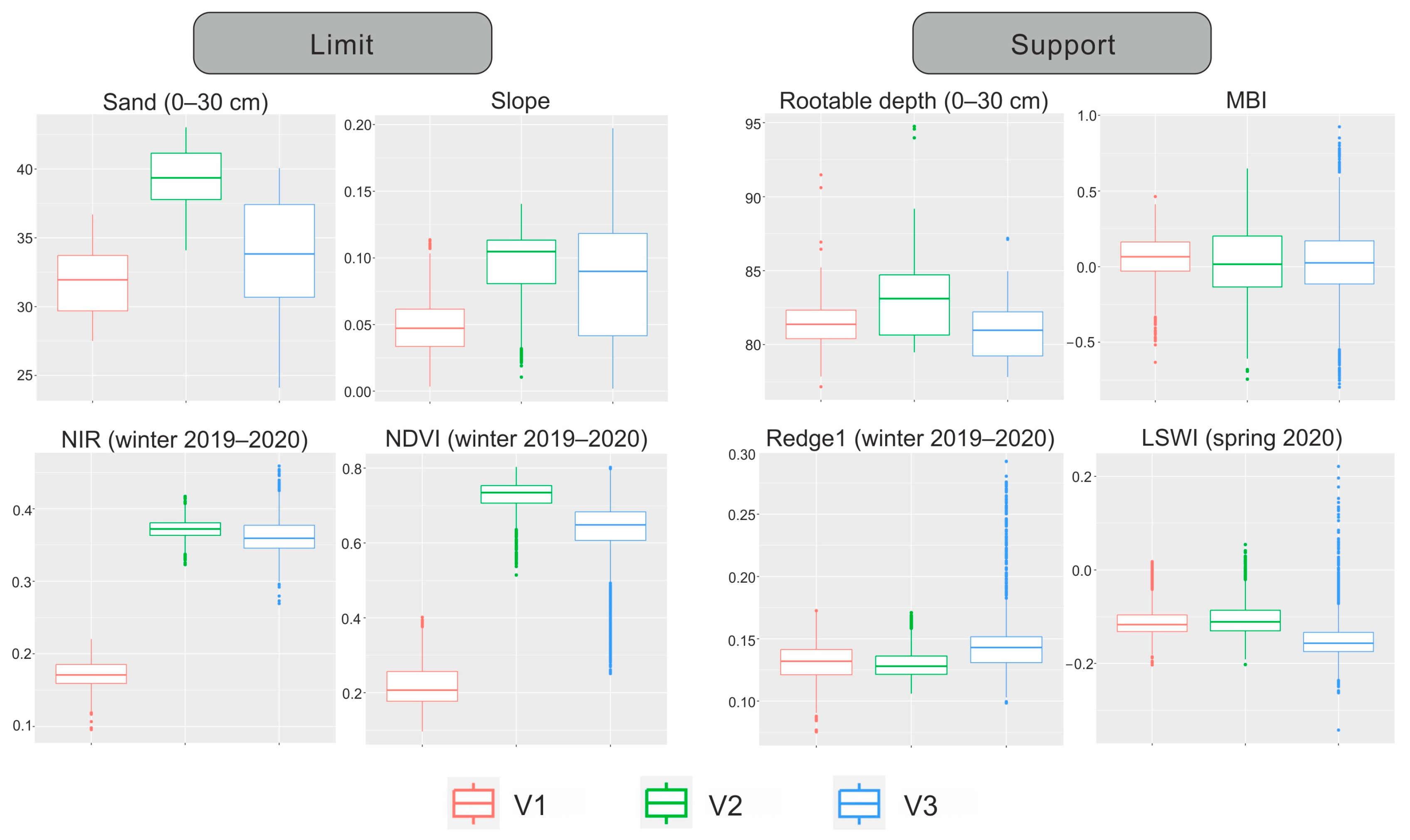
3.1. Predictor-Based Comparison of the Three Vineyards

As a first step, a comparison of the three study sites was evaluated according to environmental covariates (Supplementary Figures S1–S6) in order to support the possibility of model transferability based on the characteristics of nearby vineyards. As it has been described earlier, the V1 was a newly planted parcel, while V2 was an older vineyard, and the V3 had a varied land cover. This difference is also observed when comparing the environmental auxiliary variables for multitemporal spectral bands and indices showing seasonal variations. In the case of spectral bands R, G, and B in summer, autumn, and spring, V1 is different from the other two areas, while in winter, they show a rather similar pattern. Another example is band SWIR1, where there is a smaller variation between the areas; however, differences were observed during the summer and spring. In terms of spectral indices, we observed indices (such as CI and LSWI) where the three areas are very similar almost all year round, except in winter. In this category, there can also be found variables (NDVI, TVI) that show differences due to variations in land cover.

Looking at the topographic variables, the three areas show a high degree of similarity, with the largest difference being in the extent of the elevation, which is due to the size of the sample areas. Finally, comparing the primary soil property maps, there is a slight difference in CaCO₃ content, SOM content, and rootable depth, while there is a more significant variation in fractions: clay, silt, and sand content. Overall, for most variables, V2 and V3 are more similar to each other, although V1 also shows similarities for some environmental covariates.

In Figure 4, there is a collection of auxiliary variables that limit or support the transferability of the model between areas. One of the limiting factors of predicting soil erosion is the different fraction properties of the areas (e.g., sand), which influences the erodibility of soil. Most topographic indices do not show significant differences on the three sites, but the slope presents a visible deviation in V1. For spectral information, NIR and NDVI play an important role in determining coverage, so it was no surprise that V1 showed values different from the other two areas. On the other hand, when looking at the supporting factors for model transferability, an important factor from the erosion and viticulture point of view is the rootable depth, which is similar in all three areas. The MBI shows the balance between soil mass deposited and eroded, and it was one of the most consistent indices between all three vineyards. Finally, Red Edge 1 (Redge1) was found to be an important band, as in other agriculture studies [82], and LSWI defines the land surface water that has an impact on soil erosion and also shows similar properties in each of the studied vineyards.

Overall, there were some limiting factors, which mainly appeared in the spectral information. This is primarily due to seasonal variability. However, most of the variables showed very similar properties or a slight difference between the studied vineyards. These include topographical factors, which have been identified in several studies as the most important influencing factor of soil erosion [25,27,83]. It is concluded that this comparative analysis supports the hypothesis that the ML model can be transferable between nearby vine-growing areas.

3.2. Evaluation of the Trained Models

Nowadays, the application of different ML methods (e.g., RF, SVM, DL, ANN) is emerging in soil erosion mapping. In most of the studies, ground truth was inferred from field measurements, which were used as training data [24,26]. However, there are also examples where, like in our research, a previously produced soil erosion (potential) map was used as training data [25,83]. The three selected ML methods to test the applicability of their use in determining the rate of erosion were Ranger, SVM, and XGB because they are all suitable for use in complex environmental studies. Each method has its own strengths. Ranger is a fast implementation of the RF method and is optimized for high-dimensional datasets due to its speed. It can handle noisy data and outliers while also providing outstanding robustness and accuracy [75]. On the other hand, the simplicity of SVM comes from the application of a simple linear method to the data; it offers high accuracy and robustness, especially in high-dimensional spaces. Moreover, it is also able to handle non-linear relationships [79]. XGB is a highly robust, fast, and interpretable method, especially for large datasets. It often achieves superior accuracy even when there is missing data [78].

The evaluation of soil erosion modeling by ML is summarized in

Table 5. Accuracy values of the three ML methods tested by different training areas.

Training Area	Ranger			svmLinear3			xgbLinear
	R2	RMSE	MAE	R2	RMSE	MAE	R2	RMSE	MAE
V1	0.849	6.815	3.183	0.326	17.179	10.123	0.860	7.014	3.114
V2	0.551	7.750	3.747	0.092	26.118	10.257	0.567	8.316	3.495
V3	0.875	12.146	5.916	0.189	42.225	24.173	0.844	13.651	6.613

. In a well-performing model, R² values approach 1, while the average error (RMSE and MAE) measures converge to 0. This is taken into account when evaluating the models used. Out of the three tested ML methods, the svmLinear showed the weakest performance on all three accuracy metrics. The R² values are between 0.092 and 0.326, with relatively high RMSE (17.179–42.225 t/(ha·year)) and MAE (10.123–24.173 t/(ha·year)). While the highest R² value is associated with the lowest average error value, the lowest R² value is not associated with the highest average error value. Comparing our values with other studies, a similar result on the accuracy of SVM can be observed (R² = 0.28) in Nguyen et al., 2022 [30,35], in which they studied the erosion rates of a watershed in Northern Taiwan.

Using the Ranger methods and the xgbLinear, which are both based on decision trees, much better performance was obtained. Similar accuracy metrics values were obtained for the two methods. The R² values range from 0.551 to 0.875, with RMSE (6.815–13.651 t/(ha·year)) and MAE (3.114–6.613 t/(ha·year)). For these two methods, the highest R² performances are associated with the highest average errors, but not the lowest R² values are associated with the lowest average errors. These values are close to the results of other papers [25,26,35], among them Avand et al., 2023 [25], where they also integrated an empirical model with ML methods in a watershed of Northern Iran and obtained R² = 0.93. All these studies also show that an RF-based model provides an accurate prediction for soil erosion.

Different results were obtained not only according to the different ML algorithms but also for the different training areas. The highest R² values were obtained when the model was trained on V1, followed closely by when it was trained using data from V3, and lagged when V2 was the trainer. For the other two accuracy indicators (RMSE, MAE), the best performance was achieved when V1 was the study area. As we observed the RMSE and MAE, the larger the training study site, the greater the discrepancy observed. Similar results can be detected for the xgbLinear method as for the Ranger model due to the fact that both methods are based on decision trees.

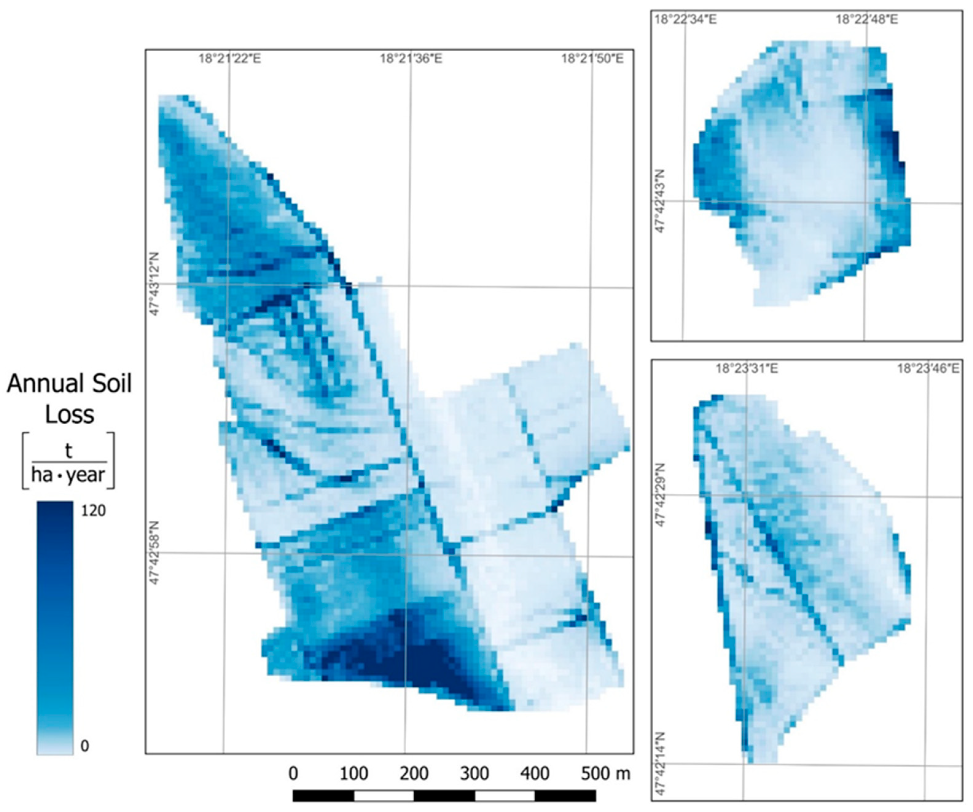
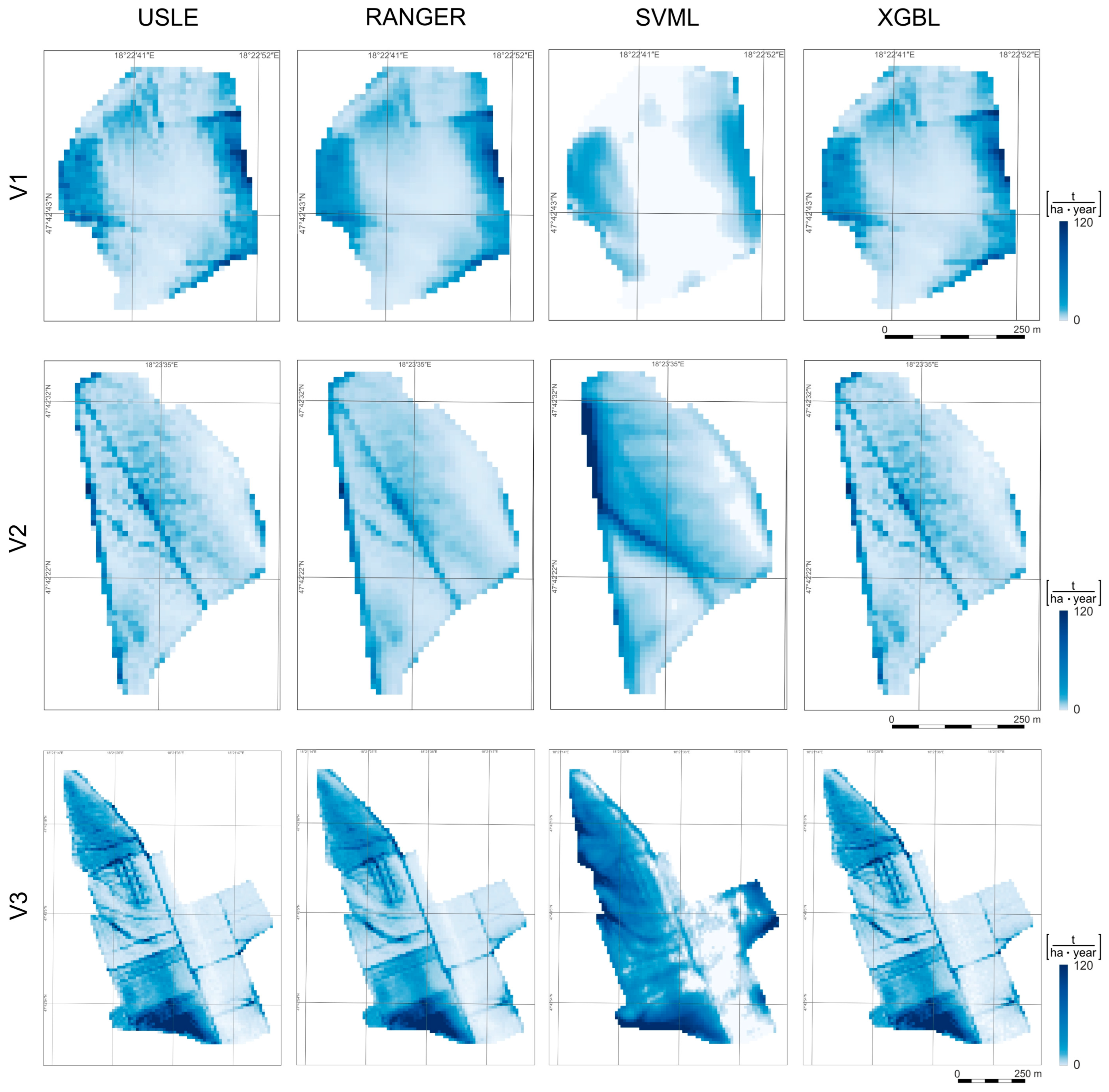
3.3. Machine Learning-Based Soil Erosion Maps

During the soil erosion mapping, the applicability of the ML methods was tested, and the resulting maps are shown in Figure 5. As seen from the accuracy metrics of the ML methods, the results of the two better-performing methods (Ranger and xgbLinear) can also be observed in the representation of the compiled maps. For both methods, we obtained a very similar erosion pattern to the map produced earlier with the USLE model. In contrast, the maps produced by the svmLinear method show weaker results than those obtained by the other two ML methods. It can be observed that the areas that are more exposed to erosion are more severe, while the areas less exposed have almost negligible erosion rates. The generated maps provide encouraging results for the applicability of ML methods based on non-observation reference data and remotely sensed geospatial information in determining the soil erosion rates.

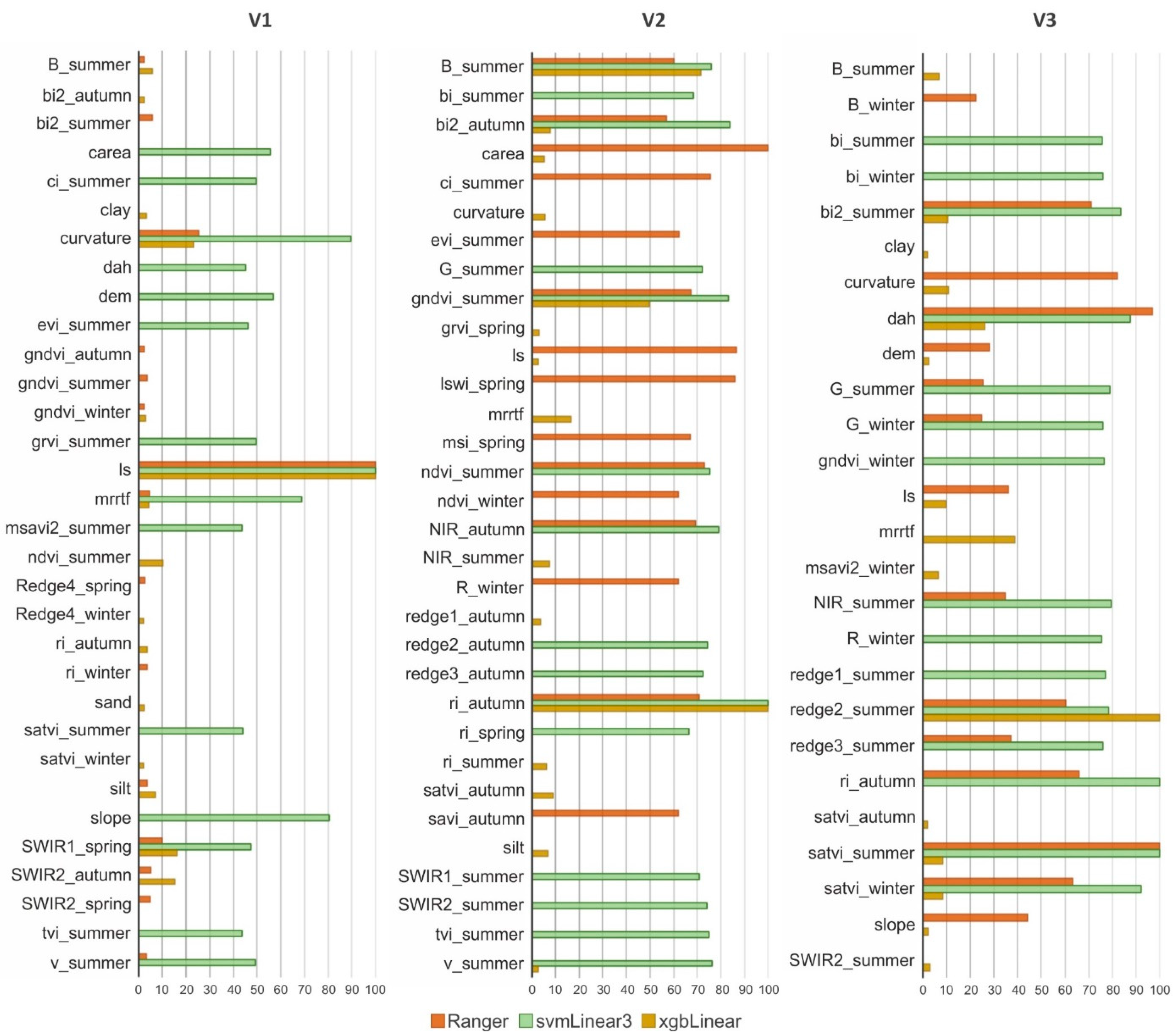
3.4. Variable Importance

Figure 6 presents the TOP 15 environmental covariates according to the various algorithms used. There was variation in predictor importance not only by study sites but also by the different ML algorithms. The highest values in the importance of environmental covariates were obtained by using the SVM method, where the lowest value was still over 75%, while in the other two decision tree-based models, values below 5% have also been found. It can also be noticed that the aspects evaluated by Ranger and xgbLinear methods show similarities. Examining the variables in terms of their nature, spectral information is the most important, followed by topomorphometric and, finally, digital soil property information.

In the case of the study sites, the variation in environmental variables in the TOP 15 was the lowest at V3, despite it having the most heterogeneous surface as well. The most significant variables for V1 (bare soil) were topographic (LS factor, curvature, MRRTF) and the spectral indices (V, NDVI, TVI), while in study areas V2 and V3, the spectral indices (SATVI, LSWI, BI2) and spectral bands (NIR, Redge 2, G) have a higher influence because they have diverse vegetation cover. Topographic variables became less dominant but still appear in the TOP 15 covariates.

These results similarly identified topographic and spectral variables, which may help determine the vegetation cover as an important variable in erosion mapping, as reported in other studies [25,26,83,84].

3.5. Evaluation of the Model Transferability

To assess our model transferability, we examined the R² and RMSE as accuracy metrics of the two maps predicted for each area, which are presented in

Table 6. Accuracy values of transferred models based on the three ML methods tested by different training areas.

Predicted for V1
	Ranger		svmLinear3		xgbLinear
Training Area	R2	RMSE	R2	RMSE	R2	RMSE
V2	0.019	27.888	0.026	33.542	0.005	62.234
V3	0.259	67.473	0.238	55.005	0.345	82.161
Predicted for V2.
	Ranger		svmLinear3		xgbLinear
Training area	R2	RMSE	R2	RMSE	R2	RMSE
V1	0.105	27.299	0.025	20.456	0.055	24.846
V3	0.068	27.535	0.101	60.555	0.019	31.537
Predicted for V3.
	Ranger		svmLinear3		xgbLinear
Training area	R2	RMSE	R2	RMSE	R2	RMSE
V1	0.338	30.123	0.173	37.280	0.332	29.484
V2	0.327	31.788	0.060	35.838	0.131	48.650

. The results of the model predictions based on the three study areas (V1, V2, and V3) show a varied performance of the ML algorithms used. In all cases, we obtained a low R² value, the highest value we obtained being 0.345. In parallel, the RMSE value was quite fluctuating, from 20.456 to 82.161 t/(ha·year).

For area V1, the results differ by an order of magnitude depending on which area was used for training. In general, a lower RMSE value was obtained when the R² value was also lower. Both the lowest R² value (0.005) and the highest R² value (0.345) with the highest RMSE (82.161 t/(ha·year)) were obtained using the xgbLinear method, which indicates poor predictive performance. The R² values for Ranger and svmLinear are almost identical, but the RMSE value depends on the training area. It is also observed that higher R² values were obtained when V3 was the study area.

The results for the V2 area predictions are also mixed. The Ranger model gave relatively low R² values (0.105; 0.068) with relatively low RMSE values (27.299 t/(ha·year); 27.535 t/(ha·year)) but still showed a better overall result than the other models. The svmLinear model gave similar R² values as in the case of prediction for V1, but a better prediction was generated with the other training area. These low R² and low RMSE indicate a less accurate prediction. The xgbLinear model also showed moderate performance.

In the case of the V3 area, the models showed relatively better performance. Here, the Ranger model achieved the highest R² value (0.338), closely followed by the xgbLinear model (0.332). The svmLinear3 model showed lower accuracy (0.173), but this result is still better than the predictions made for V1 and V2. The RMSE ranges between 29.484 and 48.650 t/(ha·year), which is also the most favorable of the three cases.

The results show that the Ranger model is the most reliable for all three areas, especially for the predictions of area V3. The xgbLinear model also performed relatively well, particularly for Area V3, while the svmLinear3 model gave generally weaker predictions.

Testing model transferability is a new research area in environmental studies. Our results can be compared to the study of mapping susceptibility of ephemeral gullies in an agricultural area in Southern Ontario, Canada [35]. Our result indicated that the best-performing method is the Ranger, which is a model based on the mentioned study. When comparing the best-performing algorithm, similar results were obtained for the inner accuracy of the models, but when testing the accuracy of the model transfer, we did not reach the accuracy achieved by them (0.57–0.76). This relatively weak result may be due to the fact that we worked with much smaller study sites.

3.6. Soil Loss Maps Produced by Model Transferability

In the frame of model transfer, where the model was trained on one of the sites and generated soil erosion estimations for the other sites. Finally, as there were three nearby areas, two estimates were made for each study area, and their average as an ensemble was used to produce final soil loss maps (Figure 7). The significant erosion patterns (e.g., major watercourses) can be identified in all of the ML-based erosion rate maps. Among the maps produced using model transfer, we can conclude that the maps generated for V3 are the most similar to the initial USLE maps in their erosion pattern. The probable reason for this is that V3 is the most diverse area; thus, both study sites from which estimates were made have some similar characteristics.

Our results are in agreement with Avand, 2023 [25], that combining the USLE/RUSLE maps and ML algorithms facilitates erosion mapping by showing areas of high erosion rates, even if these results are estimates and not exact measurements. These results are important because they can be used as a guide for land use zoning and developing appropriate and necessary management activities in erosion reduction.

To help the interpretation of the results, Figure 8 presents where the model underestimates or overestimates relative to the USLE prediction by showing the difference between each ML-based map and the USLE-based map. Overall, the highest value of overestimation appears in V1, while the largest rate of underestimation occurred in V3. A possible reason for this tendency in the case of V1 is that the two trainer areas forming the basis of the model varied greatly in terms of the environmental covariates. On the other hand, in the case of V3, one of the two trainer areas was more similar, while the other was less similar to it. Here, the underestimation exceeds the values of the overestimation. Although xgbLinear performed best in terms of the accuracy of the model, it had the highest rate of under- and overestimation, too. While the svmLinear, which produced the worst accuracy in most cases, showed the smallest deviation during the study of difference. In all cases, the largest differences are in the areas with the highest soil erosion potential. These areas of high potential soil erosion risk are in the same location as observed during the fieldwork and were also mentioned by the owner and cultivator during personal meetings. It has occurred here because one of the influencing factors of soil erosion is prominent, e.g., inappropriate cultivation techniques, lack of vegetation cover, and even a major gully can develop.

4. Conclusions

Recently, ML techniques have become increasingly popular in the field of digital mapping problems. However, there are still many questions to be answered in their application. The aim of the presented study was to test the applicability and performance of ML-based geospatial models for predicting soil erosion for the substitution of empirical models. A further aim was to test the application of the transferability of newly developed models to nearby vineyards. The performance of the following ML-based methods has been evaluated: Ranger, svmLinear, and xgbLinear.

Based on our results, the following conclusions were reached:

• The applicability of data-driven geospatial models proved to be successful in predicting soil erosion in three studied vineyards using non-observation-based reference datasets for the calibration derived from previously elaborated spatial soil loss predictions.
• Similarity analysis is important for model transferability, which is reflected in the results. The ensemble predictions gave more accurate results for the two similar areas. Despite the fact that the ML-generated soil erosion maps estimated a higher rate of degradation than the USLE-based maps, they reproduce the more significant erosion patterns, so areas more exposed to erosion can be delineated.
• Observing the inner accuracy of the constructed model, the accuracy metrics values strongly depend on the study site and the applied ML method. The best results were obtained for the most homogeneous and the most diverse area, with the better ML methods (Ranger, xgbLinear) achieving R² values as high as 0.85. On the other hand, the SVM method performed the worst in none of the areas, reaching R² = 0.4.
• Concerning the importance of environmental ancillary variables, for the area with bare soil, the topographic variables are more significant, while for the other two areas with vegetation (in our case, vines and grass between the rows of vines), the spectral indices and bands are more informative. Information on soil properties is rarely among the most important auxiliary variables, which may be due to the lower spatial resolution of the applied soil data.
• In the case of transferred models (between the study sites), lower values were obtained in the accuracy metrics. Only in a few cases was R² = 0.3 reached, but even cases with R² < 0.01 occurred.

These results suggest that model transfer between nearby study sites—even if they show similar characteristics in some environmental parameters—cannot be really established, and its feasibility still requires further research.

References

1. Kertész, Á. The global problem of land degradation and desertification. Hung. Geogr. Bull. 2009, 58, 19–31. [Google Scholar]
2. Gobin, A.; Govers, G.; Jones, R.; Kirkby, M.; Kosmas, C.; Gentile, A.R. Assessment and reporting on soil erosion. Eur. Environ. Agency Tech. Rep. 2003, 94, 103. [Google Scholar]
3. Rodrigo-Comino, J.; Keesstra, S.; Cerdà, A.A. Soil erosion as an environmental concern in vineyards: The case study of Celler del Roure, Eastern Spain, by means of rainfall simulation experiments. Beverages 2018, 4, 31. [Google Scholar] [CrossRef]
4. FAO. Provisional Methodology for Soil Degradation Assessment; FAO-UNEP-UNESCO: Rome, Italy, 1979. [Google Scholar]
5. Pool, R.; Dunst, R.; Lakso, A. Comparison of sod, mulch, cultivation, and herbicide floor management practices for grape production in nonirrigated vineyards. J. Am. Soc. Hortic. Sci. 1990, 115, 872–877. [Google Scholar] [CrossRef]
6. Biddoccu, M.; Ferraris, S.; Pitacco, A.; Cavallo, E. Temporal variability of soil management effects on soil hydrological properties, runoff and erosion at the field scale in a hillslope vineyard, North-West Italy. Soil Tillage Res. 2017, 165, 46–58. [Google Scholar] [CrossRef]
7. Batista PV, G.; Davies, J.; Silva ML, N.; Quinton, J.N. On the evaluation of soil erosion models: Are we doing enough? Earth-Sci. Rev. 2019, 197, 102898. [Google Scholar] [CrossRef]
8. Wischmeier, W.; Smith, D. Predicting Rainfall Erosion Losses. In USDA Agricultural Research Services Handbook 537; USDA: Washington, DC, USA, 1978. [Google Scholar]
9. Renard, K.; Foster, G.; Weesies, G.; Porter, J. RUSLE: Revised universal soil loss equation. J. Soil Water Conserv. 1991, 46, 30–33. [Google Scholar]
10. Christine, A.; Pasquale, B.; Katrin, M.; Panagos, P. Using the USLE: Chances, challenges and limitations of soil erosion modelling. Int. Soil Water Conserv. Res. 2019, 7, 203–225. [Google Scholar] [CrossRef]
11. Pijl, A.; Reuter, L.E.; Quarella, E.; Teun, V.A.; Tarolli, P. GIS-based soil erosion modelling under various steep-slope vineyard practices. Catena 2020, 193, 104604. [Google Scholar] [CrossRef]
12. Peter, K.D.; d’Oleire-Oltmanns, S.; Ries, J.B.; Marzolff, I.; Hssaine, A.A. Soil erosion in gully catchments affected by land-levelling measures in the Souss Basin, Morocco, analysed by rainfall simulation and UAV remote sensing data. Catena 2014, 113, 24–40. [Google Scholar] [CrossRef]
13. Fernández, T.; Pérez-García, J.L.; Gómez-López, J.M.; Cardenal, J.; Calero, J.; Sánchez-Gómez, M.; Tovar-Pescador, J. Multitemporal Analysis of Gully Erosion in Olive Groves by Means of Digital Elevation Models Obtained with Aerial Photogrammetric and LiDAR Data. ISPRS Int. J. Geo-Inf. 2020, 9, 260. [Google Scholar] [CrossRef]
14. Meinen, B.U.; Robinson, D.T. Agricultural erosion modelling: Evaluating USLE and WEPP field-scale erosion estimates using UAV time-series data. Environ. Model. Softw. 2021, 137, 104962. [Google Scholar] [CrossRef]
15. Kirkby, M.; Jones, R.; Irvine, B.; Gobin, A.; Govers, G.; Cerdan, O.; Huting, J. Pan-European Soil Erosion Risk Assessment for Europe: The PESERA Map, Version 1 October 2003; Explanation of Special Publication Ispra 2004 No. 73 (SPI 04.73); Office for Official Publications of the European Communities: Luxembourg, 2004; No. 16, 21176. [Google Scholar]
16. Lubos, M.; Mitasova, H. Distributed soil erosion simulation for effective erosion prevention. Water Resour. Res. 1998, 34, 505–516. [Google Scholar] [CrossRef]
17. Pásztor, L.; Waltner, I.; Centeri, C.; Belényesi, M.; Takács, K. Soil erosion of Hungary assessed by spatially explicit modelling. J. Maps 2016, 12 (Suppl. 1), 407–414. [Google Scholar] [CrossRef]
18. Waltner, I.; Pásztor, L.; Centeri, C.; Takács, K.; Pirkó, B.; Koós, S.; László, P. Evaluating the new soil erosion map of Hungary—A semiquantitative approach. Land Degrad. Dev. 2018, 29, 1295–1302. [Google Scholar] [CrossRef]
19. Waltner, I.; Saeidi, S.; Grósz, J.; Centeri, C.; Laborczi, A.; Pásztor, L. Spatial assessment of the effects of land cover change on soil erosion in Hungary from 1990 to 2018. ISPRS Int. J. Geo-Inf. 2020, 9, 667. [Google Scholar] [CrossRef]
20. Benavidez, R.; Jackson, B.; Maxwell, D.; Norton, K. A review of the (Revised) Universal Soil Loss Equation ((R) USLE): With a view to increasing its global applicability and improving soil loss estimates. Hydrol. Earth Syst. Sci. 2018, 22, 6059–6086. [Google Scholar] [CrossRef]
21. Koldasbayeva, D.; Tregubova, P.; Gasanov, M.; Zaytsev, A.; Petrovskaia, A.; Burnaev, E. Challenges in data-driven geospatial modeling for environmental research and practice. Nat. Commun. 2024, 15, 10700. [Google Scholar] [CrossRef]
22. McBratney, A.; Santos, M.; Minasny, B. On digital soil mapping. Geoderma 2003, 117, 3–52. [Google Scholar] [CrossRef]
23. Padarian, J.; Minasny, B.; McBratney, A. Machine learning and soil sciences: A review aided by machine learning tools. Soil 2020, 6, 35–52. [Google Scholar] [CrossRef]
24. Chen, G.; Zhao, J.; Duan, X.; Tang, B.; Zou, L.; Wang, X.; Guo, Q. Spatial Quantification of Cropland Soil Erosion Dynamics in the Yunnan Plateau Based on Sampling Survey and Multi-Source LUCC Data. Remote Sens. 2024, 16, 977. [Google Scholar] [CrossRef]
25. Avand, M.; Mohammadi, M.; Mirchooli, F.; Kavian, A.; Tiefenbacher, J.P. A New Approach for Smart Soil Erosion Modeling: Integration of Empirical and Machine-Learning Models. Environ. Model. Assess. 2023, 28, 145–160. [Google Scholar] [CrossRef]
26. Sahour, H.; Gholami, V.; Vazifedan, M.; Saeedi, S. Machine learning applications for water-induced soil erosion modeling and mapping. Soil Tillage Res. 2021, 211, 105032. [Google Scholar] [CrossRef]
27. Nguyen, K.A.; Chen, W. DEM-and GIS-Based Analysis of Soil Erosion Depth Using Machine Learning. ISPRS Int. J. Geo-Inf. 2021, 10, 452. [Google Scholar] [CrossRef]
28. Bag, R.; Mondal, I.; Dehbozorgi, M.; Bank, S.; Das, D.; Bandyopadhyay, J.; Nguyen, X. Modelling and mapping of soil erosion susceptibility using machine learning in a tropical hot sub-humid environment. J. Clean. Prod. 2022, 364, 132428. [Google Scholar] [CrossRef]
29. Mokarram, M.; Zarei, A. Soil erosion prediction using Markov and CA-Markov chains methods and remote sensing drought indicators. Ecol. Inform. 2023, 78, 102386. [Google Scholar] [CrossRef]
30. Nguyen, K.; Chen, W.; Lin, B.-S.; Seeboonruang, U. Using Machine Learning-Based Algorithms to Analyze Erosion Rates of a Watershed in Northern Taiwan. Sustainability 2022, 12, 2022. [Google Scholar] [CrossRef]
31. Senanayake, S.; Pradhan, B.; Alamri, A.; Park, H. A new application of deep neural network (LSTM) and RUSLE models in soil erosion prediction. Sci. Total Environ. 2022, 845, 157220. [Google Scholar] [CrossRef]
32. Fernández, D.; Adermann, E.; Pizzolato, M.; Pechenkin, R.; Rodríguez, C.; Taravat, A. Comparative Analysis of Machine Learning Algorithms for Soil Erosion Modelling Based on Remotely Sensed Data. Remote Sens. 2023, 15, 482. [Google Scholar] [CrossRef]
33. Folharini, S.; Vieira, A.; Bento-Gonçalves, A.; Silva, S.; Marques, T.; Novais, J. Soil erosion quantification using Machine Learning in sub-watersheds of Northern Portugal. Hydrology 2023, 10, 7. [Google Scholar] [CrossRef]
34. Takáts, T.; Mészáros, J.; Albert, G. Spatial Modelling of Vineyard Erosion in the Neszmély Wine Region, Hungary Using Proximal Sensing. Remote Sens. 2022, 14, 3463. [Google Scholar] [CrossRef]
35. Mohebzadeh, H.; Biswas, A.; DeVries, B.; Rudra, R.; Daggupati, P. Transferability of predictive models to map susceptibility of ephemeral gullies at large scale. Nat. Hazards 2024, 120, 4527–4561. [Google Scholar] [CrossRef]
36. Bihari, Z.; Babolcsai, G.; Bartholy, J.; Ferenczi, Z.; Kerényi, J.; Haszpra, L.; Homoki-Ujváry, K.; Kovács, T.; Lakatos, M.; Németh, Á.; et al. Climate in National Atlas of Hungary: Natural Environment; Kocsis, K., Ed.; MTA CSFK Geographical Institute: Budapest, Hungary, 2018; pp. 58–68. [Google Scholar]
37. IUSS Working Group WRB. World Reference Base for Soil Resources 2014: International Soil Classification System for Naming Soils and Creating Legends for Soil Maps; Update 2015; World Soil Resources Reports No. 106; FAO: Rome, Italy, 2015. [Google Scholar]
38. Pásztor, L.; Dobos, E.; Michéli, E.; Várallyay, G. Soils. In National Atlas of Hungary: Natural Environment; Kocsis, K., Ed.; MTA CSFK Geographical Institute: Budapest, Hungary, 2018; pp. 82–92. [Google Scholar]
39. Pásztor, L.; Laborczi, A.; Takács, K.; Illés, G.; Szabó, J.; Szatmári, G. Progress in the elaboration of GSM conform DSM products and their functional utilization in Hungary. Geoderma Reg. 2020, 21, e00269. [Google Scholar] [CrossRef]
40. Takáts, T. Talajerózió és Üledékfelhalmozódás Térképezése Távérzékelési Adatok Alapján. BSc Thesis, Eötvös Loránd University, Budapest, Hungary, 2018. [Google Scholar]
41. Gerzsenyi, D.; Albert, G. Landslide inventory validation and susceptibility mapping in the Gerecse Hills, Hungary. Geo-Spat. Inf. Sci. 2021, 24, 498–508. [Google Scholar] [CrossRef]
42. Demattê; JA, M.; Fongaro, C.T.; Rizzo, R.; Safanelli, J.L. Geospatial Soil Sensing System (GEOS3): A powerful data mining procedure to retrieve soil spectral reflectance from satellite images. Remote Sens. Environ. 2018, 212, 161–175. [Google Scholar] [CrossRef]
43. Escadafal, R. Remote sensing of arid soil surface color with Landsat thematic mapper. Adv. Space Res. 1989, 9, 159–163. [Google Scholar] [CrossRef]
44. Parenteau, M.; Bannari, A.; El-Harti, A.; Bachaoui, M.; EL-Ghmari, A. Characterization of the State of Soil Degradation by Erosion Using the Hue and Coloration Indices. IGARSS 2003. In Proceedings of the 2003 IEEE International Geoscience and Remote Sensing Symposium, Toulouse, France, 21–25 July 2003; IEEE Cat. No. 03CH37477. IEEE: Piscataway, NJ, USA, 2003; Volume 4, pp. 2284–2286. [Google Scholar] [CrossRef]
45. Huete, A.; Didan, K.; MODIS Science Team Members; Leeuwen, W. MODIS vegetation index (MOD13). Algorithm Theor. Basis Doc. 1999, 3, 295–309. [Google Scholar]
46. Buschmann, C.; Nagel, E. In vivo spectroscopy and internal optics of leaves as basis for remote sensing of vegetation. Int. J. Remote Sens. 1993, 14, 711–722. [Google Scholar] [CrossRef]
47. Tucker, C. Red and photographic infrared linear combinations for monitoring vegetation. Remote Sens. Environ. 1979, 8, 127–150. [Google Scholar] [CrossRef]
48. Xiao, X.; Zhang, Q.; Braswell, B.; Urbanski, S.; Boles, S.; Wofsy, S.; Ojima, D. Modeling gross primary production of temperate deciduous broadleaf forest using satellite images and climate data. Remote Sens. Environ. 2004, 91, 256–270. [Google Scholar] [CrossRef]
49. Qi, J.; Chehbouni, A.; Huete, A.; Kerr, Y.; Sorooshian, S. A modified soil adjusted vegetation index. Remote Sens. Environ. 1994, 48, 119–126. [Google Scholar] [CrossRef]
50. Hunt, E.R., Jr.; Rock, B.N. Detection of changes in leaf water content using Near- and Middle-Infrared reflectances. Remote Sens. Environ. 1989, 30, 43–54. [Google Scholar] [CrossRef]
51. Baret, F.; Guyot, G.; Major, D.J. Crop biomass evaluation using radiometric measurements. Photogrammetria 1989, 43, 241–256. [Google Scholar] [CrossRef]
52. Bannari, A.; Morin, D.; Bonn, F.; Huete, A. A review of vegetation indices. Remote Sens. Rev. 1995, 13, 95–120. [Google Scholar] [CrossRef]
53. Marsett, R.C.; Qi, J.; Heilman, P.; Biedenbender, S.H.; Watson, M.C.; Amer, S.; Marsett, R. Remote Sensing for Grassland Management in the Arid Southwest. Rangel. Ecol. Manag. 2006, 59, 530–540. [Google Scholar] [CrossRef]
54. Huete, A. A soil-adjusted vegetation index (SAVI). Remote Sens. Environ. 1988, 25, 295–309. [Google Scholar] [CrossRef]
55. Rouse, J., Jr.; Haas, R.; Schell, J.; Deering, D.; Harlan, J. Monitoring the Vernal ADVANCEMENT and Retrogradation (Green Wave EFFECT) of Natural Vegetation (No. E75-10354); Texas A&M University, Remotes Sensing Center: College Station, TX, USA, 1974. [Google Scholar]
56. Jordan, C.F. Derivation of leaf area index from quality of light on the forest floor. Ecology 1969, 50, 663–666. [Google Scholar] [CrossRef]
57. Brenning, A.; Bangs, D. Introduction to Terrain Analysis with RSAGA: Landslide Susceptibility Modeling. 2022. Available online: https://cran.r-project.org/web/packages/RSAGA/vignettes/RSAGA.html (accessed on 10 January 2025).
58. Zevenbergen, L.W.; Thorne, C.R. Quantitative analysis of land surface topography. Earth Surf. Process. Landf. 1987, 12, 47–56. [Google Scholar] [CrossRef]
59. Freeman, G.T. Calculating catchment area with divergent flow based on a regular grid. Comput. Geosci. 1991, 17, 413–422. [Google Scholar] [CrossRef]
60. Boehner, J.; Koethe, R.; Conrad, O.; Gross, J.; Ringeler, A.; Selige, T. Soil Regionalisation by Means of Terrain Analysis and Process Parameterisation. In Soil Classification 2001; Micheli, E.N., Ed.; Research Report No. 7, EUR 20398 EN; European Soil Bureau: Luxembourg, 2002; pp. 2013–2222. [Google Scholar]
61. Boehner, J.; Antonic, O. Land-surface parameters specific to topo-climatology. Dev. Soil Sci. 2009, 33, 195–226. [Google Scholar] [CrossRef]
62. Moore, I.D.; Turner, K.K.; Wilson, J.P.; Jenson, S.K.; Band, L.E. GIS and land-surface-subsurface process modeling. Environ. Model. GIS 1993, 20, 196–230. [Google Scholar]
63. Moeller, M.; Volk, M.; Friedrich, K.; Lymburner, L. Placing soil-genesis and transport processes into a landscape context: A multiscale terrain-analysis approach. J. Plant Nutr. Soil Sci. 2008, 171, 419–430. [Google Scholar] [CrossRef]
64. Gallant, J.C.; Dowling, T.I. A multiresolution index of valley bottom flatness for mapping depositional areas. Water Resour. Res. 2003, 39, 2002WR001426. [Google Scholar] [CrossRef]
65. Beven, K.J.; Kirkby, M.J. A physically based, variable contributing area model of basin hydrology/Un modèle à base physique de zone d’appel variable de l’hydrologie du bassin versant. Hydrol. Sci. J. 1979, 24, 43–69. [Google Scholar] [CrossRef]
66. Malone, B.P.; McBratney, A.B.; Minasny, B.; Wheeler, I. A general method for downscaling earth resource information. Comput. Geosci. 2012, 41, 119–125. [Google Scholar] [CrossRef]
67. Odgers, N.P.; Sun, W.; McBratney, A.B.; Minasny, B.; Clifford, D. Disaggregating and harmonising soil map units through resampled classification trees. Geoderma 2014, 214, 91–100. [Google Scholar] [CrossRef]
68. Pásztor, L.; Laborczi, A.; Takács, K.; Szatmári, G.; Dobos, E.; Bakacsi, Z.; Szabó, J. Compilation of novel and renewed, goal oriented digital soil maps using geostatistical and data mining tools. Hung. Geogr. Bull. 2015, 64, 49–64. [Google Scholar] [CrossRef]
69. Roudier, P.; Malone, B.P.; Hedley, C.B.; Minasny, B.; McBratney, A.B. Comparison of regression methods for spatial downscaling of soil organic carbon stocks maps. Comput. Electron. Agric. 2017, 142, 91–100. [Google Scholar] [CrossRef]
70. Gagkas, Z.; Lilly, A. Downscaling soil hydrological mapping used to predict catchment hydrological response with random forests. Geoderma 2019, 341, 216–235. [Google Scholar] [CrossRef]
71. Møller, A.B.; Koganti, T.; Beucher, A.; Iversen, B.V.; Greve, M.H. Downscaling digital soil maps using electromagnetic induction and aerial imagery. Geoderma 2021, 385, 114852. [Google Scholar] [CrossRef]
72. Team R Core. R: A Language and Environment for Statistical Computing; R Foundation for Statistical Computing: Vienna, Austria, 2021; Available online: https://www.R-project.org (accessed on 10 January 2025).
73. Kuhn, M. Building Predictive Models in R Using the caret Package. J. Stat. Softw. 2008, 28, 1–26. [Google Scholar] [CrossRef]
74. Kuhn, M. The Caret Package. 2019. Available online: https://topepo.github.io/caret/ (accessed on 1 December 2024).
75. Moon, J.; Park, S.; Rho, A.; Hwang, E. Robust building energy consumption forecasting using an online learning approach with R ranger. J. Build. Eng. 2022, 47, 103851. [Google Scholar] [CrossRef]
76. Breiman, L. Random forests. Mach. Learn. 2001, 45, 5–32. [Google Scholar] [CrossRef]
77. Chen, T.; Guestrin, C. XGBoost: A Scalable Tree Boosting System. In Proceedings of the 22nd ACM SIGKDD International Conference on Knowledge Discovery and Data Mining, San Francisco, CA, USA, 13–17 August 2016; pp. 785–794. [Google Scholar] [CrossRef]
78. Friedman, J. Greedy Function Approximation: A Gradient Boosting Machine. Ann. Stat. 2001, 29, 1189–1232. [Google Scholar] [CrossRef]
79. Karatzoglou, A.; Meyer, D.; Hornik, K. Support Vector Machines in R. J. Stat. Softw. 2006, 15, 1–28. [Google Scholar] [CrossRef]
80. Chicco, D.; Warrens, M.; Jurman, G. The coefficient of determination R-squared is more informative than SMAPE, MAE, MAPE, MSE and RMSE in regression analysis evaluation. PeerJ Comput. Sci. 2021, 7, e623. [Google Scholar] [CrossRef]
81. Willmott, C.; Matsuura, K. Advantages of the mean absolute error (MAE) over the root mean square error (RMSE) in assessing average model performance. Clim. Res. 2005, 30, 79–82. [Google Scholar] [CrossRef]
82. Su, J.; Yi, D.; Su, B.; Mi, Z.; Liu, C.; Hu, X.; Chen, W.-H. Aerial visual perception in smart farming: Field study of wheat yellow rust monitoring. IEEE Trans. Ind. Inform. 2020, 17, 2242–2249. [Google Scholar] [CrossRef]
83. Saha, A.; Pal, S.; Chowdhuri, I.; Islam, A.; Roy, P.; Chakrabortty, R. Land degradation risk dynamics assessment in red and lateritic zones of eastern plateau, India: A combine approach of K-fold CV, data mining and field validation. Ecol. Inform. 2022, 69, 101653. [Google Scholar] [CrossRef]
84. Kucuker, D.; Giraldo, D. Assesment of soil erosion risk using an integrated approach of GIS and Analytic Hierarchy Process (AHP) in Erzurum, Turkiye. Ecol. Inform. 2022, 71, 101788. [Google Scholar] [CrossRef]
Figure 1. Location of the three vineyards (with the Hungarian names) in Central Europe (marked with numbers).
Land 14 00163 g001
Figure 2. USLE-based annual soil loss map of the three study sites aggregated to 10 m spatial resolution.
Land 14 00163 g002
Figure 3. Flowchart of the soil erosion mapping process.
Land 14 00163 g003
Figure 4. Set of environmental covariates from the comparison of the study sites, which limit or support the model transferability process.
Land 14 00163 g004
Figure 5. Annual soil degradation rates estimated by ML methods.
Land 14 00163 g005
Figure 6. TOP 15 important environmental covariates of each study site.
Land 14 00163 g006
Figure 7. Annual soil degradation rates estimated by ML methods transfer.
Land 14 00163 g007
Figure 8. Differences between the USLE-based and the ML methods estimated annual soil loss rates.
Land 14 00163 g008