


Research on Improving the Accuracy of SIF Data in Estimating Gross Primary Productivity in Arid Regions

 , ,
, ,  ,
,
Abstract
1. Introduction
2. Data and Methods
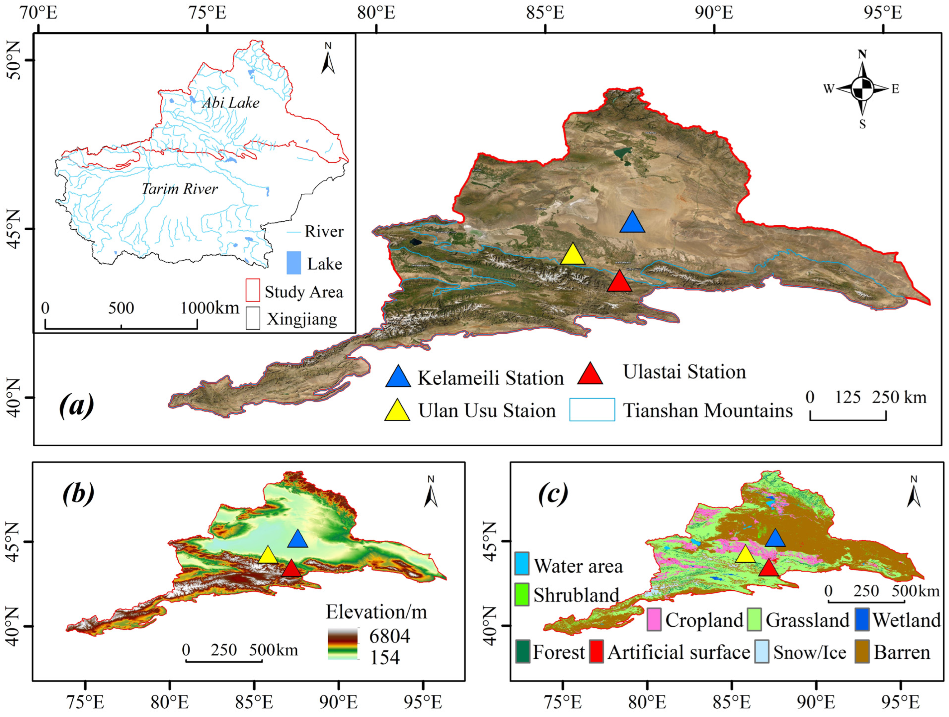
2.1. Study Area
2.2. Data Sources
2.2.1. Site Data
2.2.2. Satellite Data
2.2.3. Other Auxiliary Data
2.3. Data Processing
2.3.1. Site Data Processing
2.3.2. Satellite Data Processing
2.4. Research Methods
2.4.1. Method for Applicability Verification
2.4.2. Method for Response Degrees Verification
2.4.3. Method for GPP/SIF Verification
2.4.4. Method for SIF Precision Improvement
3. Results
3.1. GPP Various on the Site
3.2. Analysis of GPP Estimation Using Multisource SIF Satellite Products
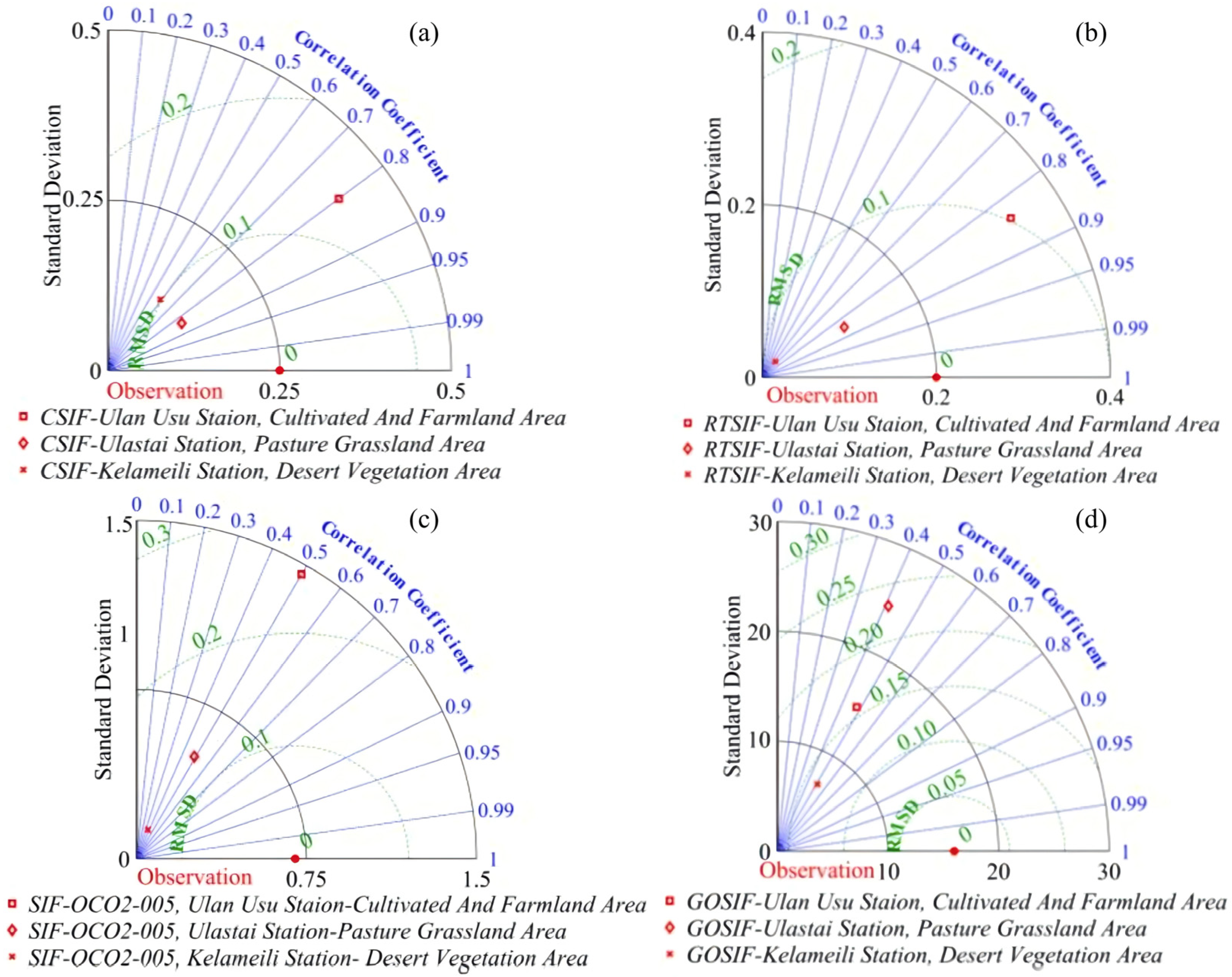
3.2.1. Analysis of Applicability
3.2.2. Analysis of Spatial Features
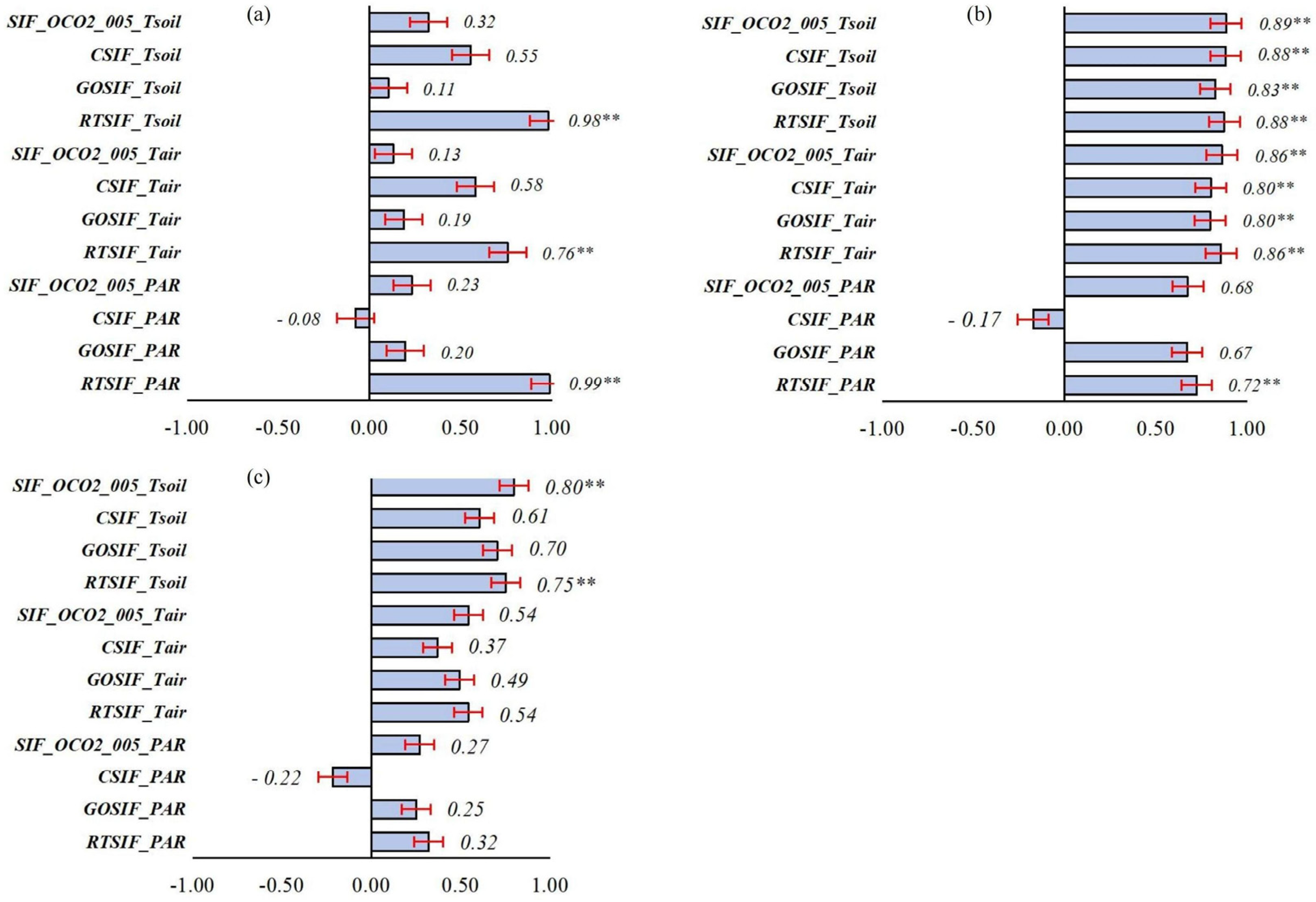
3.2.3. Analysis of the Impact Factor Responsiveness
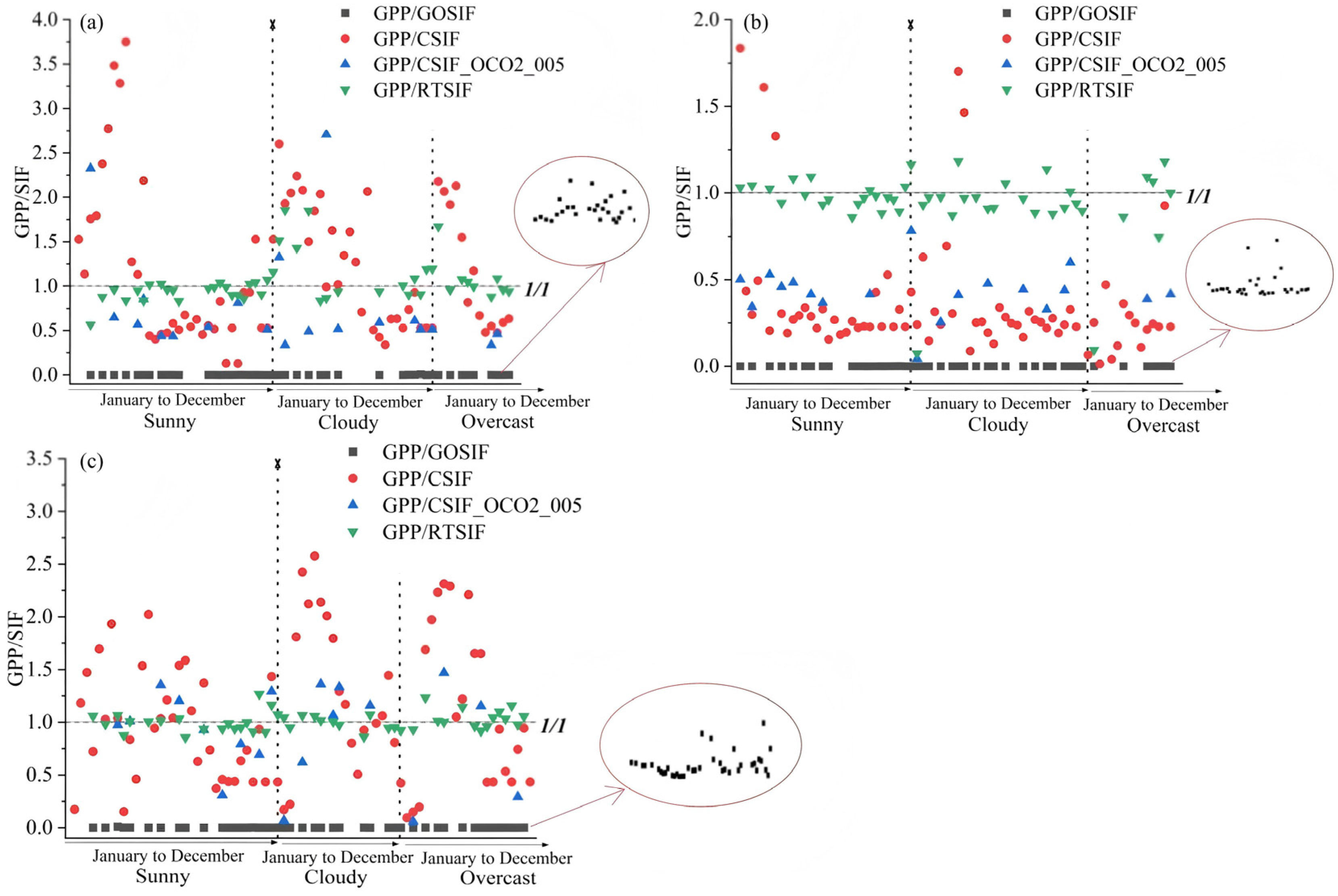
3.2.4. Analysis of GPP/SIF Values under Different Weather Conditions
3.3. SIF Data Accuracy Improvement Analysis
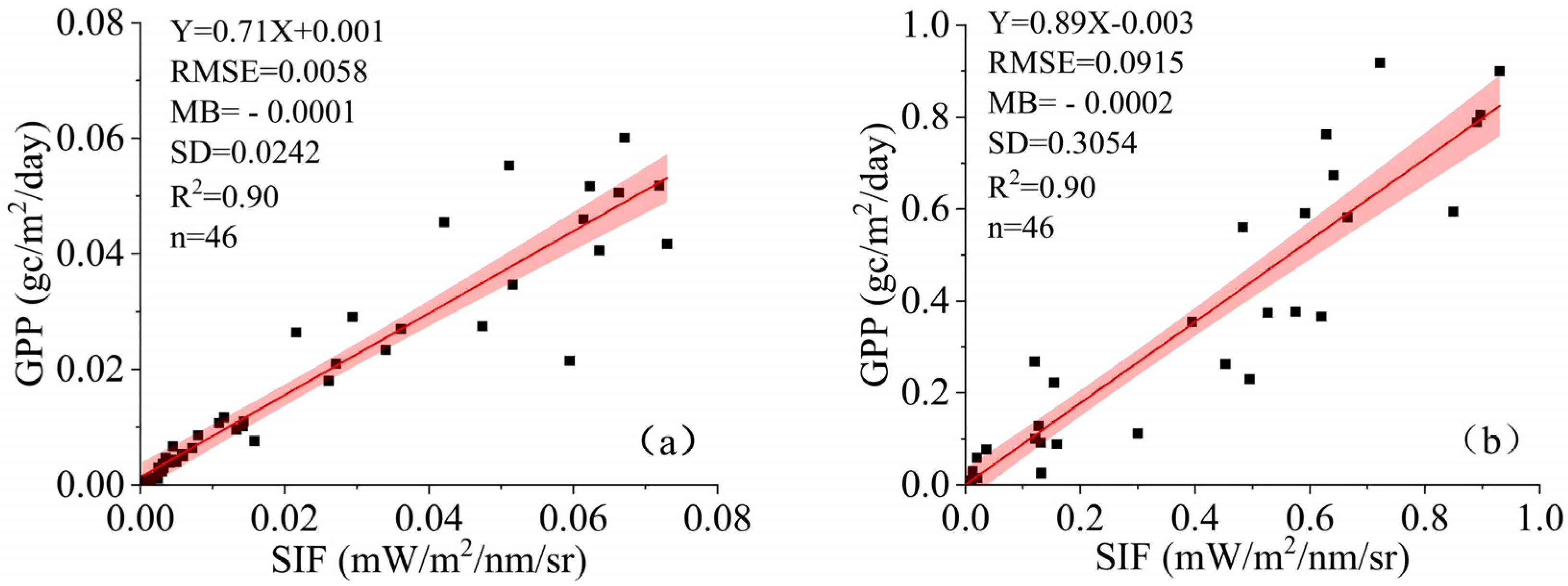
3.3.1. Analysis of Canopy-Based Accuracy Improvement
3.3.2. Analysis of Linear-Based Accuracy Improvement
3.3.3. Comparative Analysis of Accuracy improvement Based on Canopy and Linear Methods
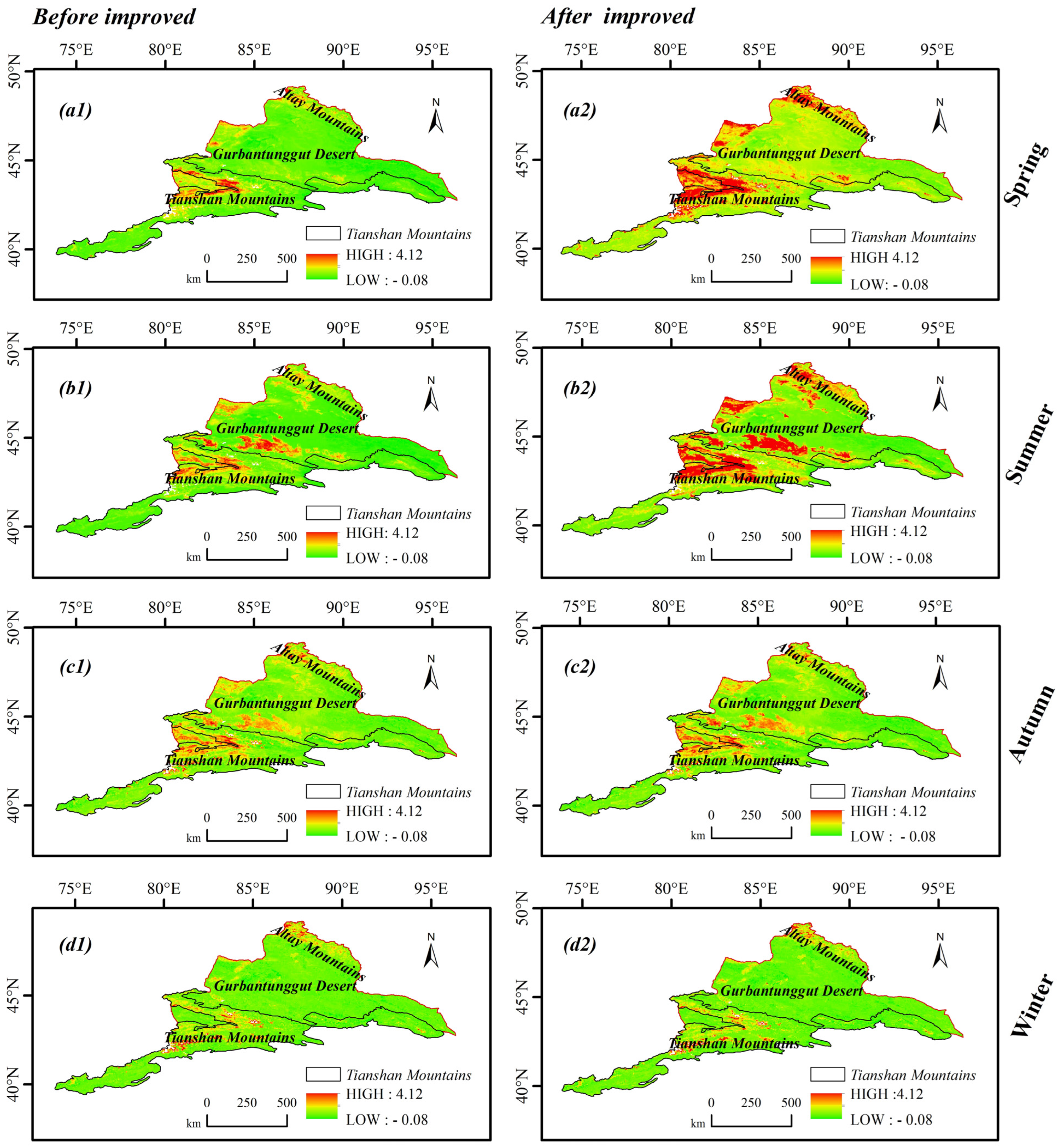
3.4. Spatial Analysis of SIF Data Accuracy Improvement before and after
4. Discussion
4.1. Analysis of the Applicability of Multisource SIF Data in Estimating GPP
4.2. Analysis of GPP Estimation Accuracy Based on Improving SIF
4.3. Innovation, Limitations, and Prospects
5. Conclusions
- (1)
- The interannual variation of the monthly mean GPP in arid regions shows an inverted “U” shape, with peaks occurring in June and July. During the growing season (March to October), GPP first increases and then decreases, while in the nongrowing season (November to February), GPP fluctuations are not significant.
- (2)
- The overall suitability ranking of multisource SIF satellite products for GPP estimation in arid regions is as follows: RTSIF > CSIF > SIF_OCO2_005 > GOSIF. This has a profound significance for revealing the spatial and temporal patterns of the terrestrial ecosystem carbon cycle in arid regions by coupling multiple factors and provides new approaches for constructing carbon reduction policies in arid regions.
- (3)
- When improving the accuracy of SIF satellite products in arid regions, both the canopy improvement method and the linear improvement method need to be used in combination. This provides practical theory for achieving a more comprehensive and higher accuracy analysis of carbon source/sink spatial and temporal characteristics in arid region terrestrial ecosystems, which is of great significance for achieving “carbon neutrality” in arid regions.
- (4)
- Based on land use data, the spatial characteristics of SIF data in arid regions achieved through the two methods showed a high correlation with vegetation coverage, with the annual mean value of SIF data for each surface after improvement being approximately 0.13 mw/m2/nm/sr.
6. Practical Applications
- (1)
- By revealing the interannual variation characteristics of GPP in arid regions, relevant theories can be directly referenced in the subsequent construction of the carbon cycle system in arid regions, thereby avoiding unreasonable interannual variations.
- (2)
- By revealing the most suitable SIF satellite products for GPP estimation in arid regions, the relevant satellites can be directly applied in subsequent analysis of the spatial and temporal patterns of carbon storage in arid regions based on GPP, an important factor of carbon source/sink, thus avoiding repeated comparative validation.
- (3)
- By revealing the methods for improving the accuracy of SIF satellite products in arid regions, these methods can be directly applied in subsequent accuracy improvement of other SIF satellite products in arid regions, thus avoiding repeated exploration and analysis.
- (4)
- By revealing the spatial characteristics of GPP indirectly reflected by SIF in arid regions, accurate carbon reduction policies can be directly constructed based on the spatial patterns to achieve “carbon neutrality” in arid regions, thus avoiding discrepancies between practice and reality.
Author Contributions
Funding
Data Availability Statement
Acknowledgments
Conflicts of Interest
References
- Anav, A.; Friedlingstein, P.; Beer, C.; Ciais, P.; Zhao, M. Spatiotemporal patterns of terrestrial gross primary production: A review. Rev. Geophys. 2015, 53, 785–818. [Google Scholar] [CrossRef]
- Jung, M.; Reichstein, M.; Margolis, H.A.; Cescatti, A.; Richardson, A.D.; Arain, M.A.; Arneth, A.; Bernhofer, C.; Bonal, D.; Chen, J.Q.; et al. Global patterns of land-atmosphere fluxes of carbon dioxide, latent heat, and sensible heat derived from eddy covariance, satellite, and meteorological observations. J. Geophys. Res. Biogeosci. 2011, 116, G3. [Google Scholar] [CrossRef]
- Garbulsky, M.F.; Filella, I.; Verger, A.; Pe Uelas, J. Photosynthetic light use efficiency from satellite sensors: From global to Mediterranean vegetation. Environ. Exp. Bot. 2014, 103, 3–11. [Google Scholar] [CrossRef]
- Zhang, X.; Wang, H.; Yan, H.; Ai, J. Remote sensing study on the spatiotemporal variation of China’s total primary productivity from 2001 to 2018. Acta Ecol. Sin. 2021, 41, 6351–6362. [Google Scholar]
- Sun, Y.; Frankenberg, C.; Jung, M.; Joiner, J.; Guanter, L.; Köhler, P.; Magney, T. Overview of Solar-Induced chlorophyll Fluorescence (SIF) from the Orbiting Carbon Observatory-2: Retrieval, cross-mission comparison, and global monitoring for GPP. Remote Sens. Environ. 2018, 209, 808–823. [Google Scholar] [CrossRef]
- Xiao, J.; Chevallier, F.; Gomez, C.; Guanter, L.; Hicke, J.A.; Huete, A.R.; Ichii, K.; Ni, W.J.; Pang, Y.; Rahman, A.F.; et al. Remote sensing of the terrestrial carbon cycle: A review of advances over 50 years. Remote Sens. Environ. 2019, 233, 111383. [Google Scholar] [CrossRef]
- Lasslop, G.; Reichstein, M.; Papale, D.; Richardson, A.D.; Arneth, A.; Barr, A.; Stoy, P.; Wohlfahrt, G. Separation of net ecosystem exchange into assimilation and respiration using a light response curve approach: Critical issues and global evaluation. Glob. Chang. Biol. 2010, 16, 187–208. [Google Scholar] [CrossRef]
- Baldocchi, D. TURNER REVIEW No.15. ‘Breathing’ of the terrestrial biosphere: Lessons learned from a global network of carbon dioxide flux measurement systems. Aust. J. Bot. 2008, 56, 1–26. [Google Scholar] [CrossRef]
- Yu, G.; Fu, Y.; Sun, X.; Wen, X.; Zhang, L. Research progress and development ideas of ChinaFLUX, the Chinese Terrestrial Ecosystem Flux Research Network. China Sci. D Earth Sci. 2006, S1, 1–21. [Google Scholar] [CrossRef]
- Huang, P. Estimation of Terrestrial Gross Primary Productivity Based on Solar-Induced Chlorophyll Fluorescence; Wuhan University of Technology: Wuhan, China, 2019. [Google Scholar]
- Tramontana, G.; Jung, M.; Schwalm, C.R.; Ichii, K.; Camps-Valls, G.; Ráduly, B.; Reichstein, M.; Arain, M.A.; Cescatti, A.; Kiely, G.; et al. Predicting carbon dioxide and energy fluxes across global FLUXNET sites with regression algorithms. Biogeosciences 2016, 13, 4291–4313. [Google Scholar] [CrossRef]
- Sun, Z.; Gao, X.; Du, S.; Liu, X. Research progress and prospect of satellite remote sensing products of solar-induced chlorophyll fluorescence. Remote Sens. Technol. Appl. 2021, 36, 1044–1056. [Google Scholar]
- Gao, H.Q.; Liu, S.G.; Lu, W.Z.; Smith, A.R.; Valbuena, R.; Yan, W.D.; Wang, Z.; Li, X.; Peng, X.; Li, Q.Y.; et al. Global Analysis of the Relationship between Reconstructed Solar-Induced Chlorophyll Fluorescence (SIF) and Gross Primary Production (GPP). Remote Sens. 2011, 13, 2824. [Google Scholar] [CrossRef]
- Wang, Y.; Chi, Y.; Zhou, L. 2007-2018 Spatiotemporal Patterns and Climatic Regulation of China’s Terrestrial Vegetation Gross Primary Production and Solar-Induced Chlorophyll Fluorescence. Remote Sens. Technol. Appl. 2022, 37, 692–701. [Google Scholar]
- Qiu, R.N.; Han, G.; Li, X.; Xiao, J.F.; Liu, J.G.; Wang, S.H.; Li, S.W.; Gong, W. Contrasting responses of relationship between solar-induced fluorescence and gross primary production to drought across aridity gradients. Remote Environ. 2024, 302, 113984. [Google Scholar] [CrossRef]
- Wei, X.; He, W.; Zhou, Y.; Ju, W.M.; Xiao, J.F.; Li, X.; Liu, Y.B.; Xu, S.H.; Bi, W.J.; Zhang, X.Y.; et al. Global assessment of lagged and cumulative effects of drought on grassland gross primary production. Ecol. Indic. 2022, 136, 108646. [Google Scholar] [CrossRef]
- Liu, X.; Lai, Q.; Yin, S.; Bao, Y.H.; Qing, S.; Mei, L.; Bu, L.X. Exploring sandy vegetation sensitivities to water storage in China’s arid and semi-arid regions. Ecol. Indic. 2022, 136, 108711. [Google Scholar] [CrossRef]
- Wang, X. Understanding Carbon Uptake Using Multi-Scale Novel Remote Sensing Techniques; The University of Arizona: Tucson, AZ, USA, 2022. [Google Scholar]
- Zhang, Y.; Joiner, J.; Alemohammad, S.H.; Zhou, S.; Gentine, P. A global spatially contiguous solar-induced fluorescence (CSIF) dataset using neural networks. Biogeosciences 2018, 15, 5779–5800. [Google Scholar] [CrossRef]
- Zhang, Y. A Global Spatially Contiguous Solar-Induced Fluorescence (CSIF) Dataset Using Neural Networks (2000–2022); National Tibetan Plateau/Third Pole Environment Data Center: Beijing, China, 2021. [Google Scholar] [CrossRef]
- Chen, X.; Huang, Y.; Nie, C.; Zhang, S.; Wang, G.Q.; Chen, S.L.; Chen, Z.C. A long-term reconstructed TROPOMI solar-induced fluorescence dataset using machine learning algorithms. Sci. Data 2023, 09, 1038. [Google Scholar] [CrossRef]
- Chen, X.; Huang, Y.; Nie, C.; Zhang, S.; Wang, G.Q.; Chen, S.L.; Chen, Z.C. Global High-Resolution (8 Days, 0.05°) Solar-Induced Fluorescence Dataset (2001–2020); National Tibetan Plateau Data Center: Beijing, China, 2022. [Google Scholar] [CrossRef]
- Li, X.; Xiao, J. A global, 0.05-degree product of solar-induced chlorophyll fluorescence derived from OCO_2, MODIS, and reanalysis data. Remote Sens. 2019, 11, 517. [Google Scholar] [CrossRef]
- Yu, L.; Wen, J.; Chang, C.Y.; Frankenberg, C.; Sun, Y. High Resolution Global Contiguous SIF Estimates from OCO_2 SIF and MODIS, 2nd ed.; ORNL DAAC: Oak Ridge, TN, USA, 2021. [Google Scholar] [CrossRef]
- An, Y.; Zhang, R.; Liu, W.; Wang, P.; Zhang, J.; Wu, L.; Sun, Z. Differential analysis of different SIF products in rubber plantation areas of Hainan Island and their impact on GPP estimation. J. Trop. Biol. 2023, 19, 074028. [Google Scholar]
- Dang, C.Y.; Shao, Z.F.; Huang, X.; Qian, J.X.; Cheng, G.; Ding, Q.; Fan, Y.W. Assessment of the importance of increasing temperature and decreasing soil moisture on global ecosystem productivity using solar-induced chlorophyll fluorescenc. Glob. Chang. Biol. 2022, 28, 2066–2080. [Google Scholar] [CrossRef] [PubMed]
- Frankenberg, C.; Berry, J. Solar Induced Chlorophyll Fluorescence: Origins, Relation to Photosynthesis and Retrieval. Compr. Remote Sens. 2018, 3, 143–162. [Google Scholar]
- Yu, L.; Wen, J.; Chang, C.Y.; Frankenberg, C.; Sun, Y.; Frankenberg, C.; Sun, Y. High-Resolution Global Contiguous SIF of OCO_2. Geophys. Res. Lett. 2019, 46, 1449–1458. [Google Scholar] [CrossRef]
- Li, J.; Pu, Z.; Zhang, S. Impact of Climate Change on Agriculture in Xinjiang and Regionalization; China Meteorological Press: Beijing, China, 2018. [Google Scholar]
- Hu, R.; Jiang, F.; Wang, Y. Environmental assessment of snow and ice water resources in Xinjiang. Arid Zone Res. 2003, 20, 187–191. [Google Scholar]
- Apar, R.; Yerkejiang, H.; Li, Q.; Huang, J.; Zhang, S.Q.; Changji Prefecture Meteorological Bureau, Xinjiang; Institute of Desert Meteorology, China Meteorological Administration, Urumqi; Xinjiang Agricultural Meteorological Observatory. Analysis of the spatial and temporal characteristics of temperature in Xinjiang. Hubei Agric. Sci. 2022, 61, 34–41. [Google Scholar]
- Zou, C.; Ji, C.; Fan, Z.; Huang, J.; Chen, D.H.; Li, B. Study on water vapor and carbon dioxide fluxes in cotton fields in Ulan Usu oasis. Chin. Agric. Sci. Bull. 2014, 30, 120–125. [Google Scholar]
- Xiao, W.Q.; Mamtimin, M.; Liu, Y.Q.; Wang, Y.; Gao, J.C.; Ajiguli, S.; Gulini, S.M. Evolution of surface radiation balance in the central Tianshan Mountains. Acta Ecol. Sin. 2022, 42, 4550–4560. [Google Scholar]
- Zhang, K.; Wang, Y.; Mamtimin, A.; Liu, Y.Q.; Gao, J.C.; Aihaiti, A.; Wen, C.; Song, M.Q.; Yang, F.; Zhou, C.L.; et al. Temporal and Spatial Variations in Carbon Flux and Their Influencing Mechanisms on the Middle Tien Shan Region Grassland Ecosystem, China. Remote Sens. 2023, 15, 4091. [Google Scholar] [CrossRef]
- Mamtimin, A. Study on Carbon Balance Characteristics and Influencing Factors in Desert Areas of Xinjiang; Nanjing University of Information Science and Technology: Nanjing, China, 2015. [Google Scholar]
- Gao, J.; Wang, Y.; Aiguli, S.; Mamtimin, A.; Liu, Y.Q.; Zhao, X.S.; Yang, X.H.; Huo, W.; Yang, F.; Zhou, C. Characteristics of surface radiation balance in Gurbantunggut Desert. Desert Res. 2021, 41, 47–58. [Google Scholar]
- Kai, Y.; Wang, J.; Weiss, M.; Myneni, R.B. A High-Quality Reprocessed MODIS Leaf Area Index Dataset (HiQ-LAI), 1st ed.; [Data Set]; Zenodo: Beijing, China, 2023. [Google Scholar] [CrossRef]
- Xu, X.; Liu, J.; Zhang, S.; Li, R.; Yan, C.; Wu, S. China’s Multi-Period Land Use Remote Sensing Monitoring Dataset (CNLUCC); Resource and Environmental Science Data Registration and Publishing System: Beijing, China, 2018. [Google Scholar]
- Long, T.F.; Jiao, W.L.; Zhang, Z.M.; He, G.J. Calculation Method of Satellite Image Pixel Observation Zenith Angle and Azimuth Angle. CN201410352963.8, 6 June 2017. [Google Scholar]
- Pan, J. Arithmetic mean, geometric mean and theta function. J. Harbin Norm. Univ. Nat. Sci. Ed. 2014, 30, 21–22. [Google Scholar]
- Feret, J.B.; Francois, C.; Asner, G.P.; Gitelson, A.A.; Martin, R.E.; Bidel, L.P.R.; Ustin, S.L.; Le Maire, G.; Jacquemoud, S. PROSPECT-4 and 5:Advances in the leaf optical properties model separating photosynthetic pigments. Remote Sens. Environ. 2011, 112, 3030–3043. [Google Scholar] [CrossRef]
- Xinjie, L.J.; Luis, G.; Liangyun, L.Y.; Damm, A.; Malenovsky, Z.; Rascher, U.; Peng, D.L.; Du, S.S.; Gastellu-Etchegorry, J.P. Downscaling of solar-induced chlorophyll fluorescence from canopy level to photosystem level using a random forest model. Remote Sens. Environ. 2018, 231, 110772. [Google Scholar] [CrossRef]
- Gueymard, C.A. Parameterized transmittance model for direct beam and circumsolar spectral irradiance. Sol. Energy 2001, 71, 325–346. [Google Scholar] [CrossRef]
- He, L.M.; Chen, J.M.; Pisek, J.; Schaaf, C.B.; Strahler, A.H. Global clumping index map derived from the MODIS BRDF product. Remote Sens. Environ. 2012, 119, 118–130. [Google Scholar] [CrossRef]
- Vickers, D.; Mahrt, L. Quality control and flux sampling problems for tower and aircraft data. J. Atmos. Ocean. Technol. 1997, 14, 512–526. [Google Scholar] [CrossRef]
- Zhuang, J.; Wang, W.; Wang, J. Calculation of eddy correlation flux and comparison analysis of three major software. Plateau Meteorol. 2013, 32, 78–87. [Google Scholar]
- Kaimal, J.C.; Finnigan, J. Atmospheric Boundary Layer Flows: Their Structure and Measurement; Oxford University Press: Oxford, UK, 1994. [Google Scholar]
- Moore, C. Frequency-response corrections for eddy-correlation systems. J. Appl. Meteorol. 1986, 37, 17–35. [Google Scholar] [CrossRef]
- Schotanus, P.; Nieuwstadt, F.T.M.; Debruin, H.A.R. Temperature-measurement with a sonic anemometer and its application to heat and moisture fluxes. Bound.-Layer Meteorol. 1983, 26, 81–93. [Google Scholar] [CrossRef]
- Zhao, N.; Zhou, L.; Zhuang, J.; Wang, Y.L.; Zhou, W.; Chen, J.J.; Song, J.; Ding, J.X.; Chi, Y.G. Integration analysis of the carbon sources and sinks in terrestrial ecosystems, China. Acta Ecol. Sin. 2021, 41, 7648–7658. [Google Scholar]
- Reichstein, M.; Falge, E.; Baldocchi, D.; Papale, D.; Valentini, R. On the separation of net ecosystem exchange into assimilation andecosystem respiration: Review and improved algorithm. Glob. Chang. Biol. 2005, 11, 1424–1439. [Google Scholar] [CrossRef]
- Gu, L.H.; Fuentes, J.D.; Shugart, H.H.; Staebler, R.M.; Black, T.A. Responses of net ecosystem exchanges of carbon dioxide to changes in cloudiness: Results from two North American deciduous forests. J. Geophys. Res. Atmos. 1999, 104, 31421–31434. [Google Scholar]
- Okogbue, E.C.; Adedokun, J.A.; Holmgren, B. Hourly and daily clearness index and diffuse fraction at a tropical station, Ile-Ife, Nigeria. Int. J. Climatol. 2009, 29, 1035. [Google Scholar] [CrossRef]
- Yang, F. Predictive Ability of Global Sun-Induced Chlorophyll Fluorescence for Vegetation Gross Primary Production and Its Response to Drought; Nanjing University of Information Science & Technology: Nanjing, China, 2022. [Google Scholar] [CrossRef]
- Glahn, H.R.; Lowry, D.A. The use of model output statistics (MOS) in objective weather forecasting. J. Appl. Meteorol. 1972, 11, 1203–1211. [Google Scholar] [CrossRef]
- Polo, J.; Wilbert, S.; Ruizarias, J.A.; Meyer, R.; Gueymard, C.A.; Suri, M.; Martin, L.; Mieslinger, T.; Blanc, P.; Grant, I. Integration of Ground Measurements with Model-Derived Data; Environmental Science, Engineering: Cambridge, MA, USA, 2015. [Google Scholar]
- Zhang, Y.L.; Yin, B.F.; Tao, Y.; Li, Y.G.; Zhou, X.B.; Zhang, Y.M. The first rainfall time in early spring and the impact of rainfall on the morphological characteristics and chlorophyll fluorescence of two short-lived plants in the Gurbantunggut Desert. J. Plant Ecol. 2022, 46, 428–439. [Google Scholar] [CrossRef]
- Han, W.; Hamiti, Y.; Li, L.; Li, S.Y.; Zheng, T.T. The response of chlorophyll fluorescence parameters and stem water potential of Populus euphratica and Populus gray to the habitat in the hinterland of the Taklamakan Desert. Chin. Desert 2011, 31, 1472–1478. [Google Scholar]
- Wu, L.Y.; Zhang, J.G.; Chang, W.Q.; Zhang, S.L.; Chang, Q. Diurnal variation characteristics of chlorophyll fluorescence parameters of three desert plants. Pratacult. Sci. 2021, 30, 203–213. [Google Scholar]
- Han, W.; Cao, L.; Haimti, Y.; Xu, X. Response of chlorophyll fluorescence of Tamarix ramosissima to dust storm weather. J. Desert Res. 2012, 32, 86–91. [Google Scholar]
- Li, L.; Li, X.Y.; Lin, L.S.; Wang, Y.J.; Xue, W. Application of chlorophyll fluorescence characteristics of 9 Poaceae forages on the photosystem II of the southern edge of the Taklimakan Desert. Acta Ecol. Sin. 2011, 22, 2599–2603. [Google Scholar]
- Frankenberg, C.; O'Dell, C.; Berry, J.; Guanter, L.; Joiner, J.; Köhler, P.; Pollock, R.; Taylor, T.E. Prospects for chlorophyll fluorescence remote sensing from the Orbiting Carbon Observatory-2. Remote Sens. Environ. 2014, 147, 1–12. [Google Scholar] [CrossRef]
- Liu, X.T.; Zhou, L.; Shi, H.; Wang, S.Q.; Chi, Y.G. Comparative analysis of phenological characteristics of temperate coniferous and broad-leaved mixed forests based on multiple remote sensing vegetation indices, chlorophyll fluorescence, and CO2 flux data. Acta Ecol. Sin. 2018, 38, 13. [Google Scholar] [CrossRef]
- Dong, T. Study on the Spatiotemporal Evolution Characteristics of Arid Climate and Its Impact on Grassland Phenology in Xinjiang. Ph.D. Thesis, Xinjiang Agricultural University, Urumqi, China, 2023. [Google Scholar]
- Chen, X. Research on Global Total Primary Productivity Estimation of Multiple Crop Types. Master’s Thesis, Nanjing University of Information Science & Technology, Nanjing, China, 2023. [Google Scholar]
- Yang, F.; Huang, J.; Zheng, X.; Zheng, X.; Huo, W.; Zhou, C.; Wang, Y.; Han, D.L.; Gao, J.C.; Mamtimin, M.; et al. Evaluation of carbon sink in the Taklimakan Desert basedon correction of abnormal negative CO2 flux of IRGASON. Sci. Total Environ. 2022, 838, 155988. [Google Scholar] [CrossRef] [PubMed]
- Amar, G.; Mamtimin, A.; Wang, Y.H.; Wang, Y.; Gao, J.C.; Yang, F.; Song, M.Q.; Aihaiti, A.; Wen, C.; Liu, J.J. Factors controlling and variations of CO2 fluxes during the growing season in Gurbantunggut Desert. Ecol. Indic. 2023, 154, 110708. [Google Scholar] [CrossRef]
- Yin, Y. Reconstruction of Global Solar-Induced Chlorophyll Fluorescence Remote Sensing Data Considering Canopy Correction. Master’s Thesis, Nanjing Normal University, Nanjing, China, 2021. [Google Scholar]
- Wang, Y.; Zhao, X.S.; Mamtimin, A.; Sayit, H.; Abulizi, S.; Maturdi, A.; Yang, F.; Huo, W.; Zhou, C.L.; Yang, X.H.; et al. Evaluation of Reanalysis Datasets for Solar Radiation with In Situ Observations at a Location over the Gobi Region of Xinjiang, China. Remote Sens. 2021, 13, 4191. [Google Scholar] [CrossRef]
- Li, Y.; Sun, Z.G. Spatiotemporal dynamics analysis of grassland productivity in the Mongolian Plateau based on remote sensing of chlorophyll fluorescence. Jiangsu Agric. Sci. 2021, 49, 219–226. [Google Scholar]
- Yan, Z.; Liu, L.Y.; Jing, X. A Study on the Temporal and Spatial Changes of Vegetation Fluorescence and Climate Response Models in China from 2007 to 2018. Remote Sens. Technol. Appl. 2022, 37, 702–712. [Google Scholar]
- Song, L. Research on Remote Sensing Monitoring of Chlorophyll Fluorescence under High-Temperature Stress of Crops. Ph.D. Thesis, Nanjing University, Nanjing, China, 2023. [Google Scholar]


| Station Name | Abbreviation | Coordinates | Elevation | Region | Underlying Surface |
|---|---|---|---|---|---|
| Ulan Usu Land-Atmosphere Interaction Observation Station | Ulan Usu Station | 44°16′59″ N 85°49′00″ E | 406.9 m | The northern slope of Tianshan Mountains | Cultivated and farmland area [32] |
| Central Tianshan Land-Atmosphere Interaction Observation Station | Ulastai Station | 43°28′55″ N 87°12′50″ E | 2036 m | The central hinterland of the Tianshan Mountains | Pasture grassland area [33,34] |
| Kelameili Land-Atmosphere Interaction Observation Station | Kelameili Station | 45°14′00″ N 87°35′00″ E | 531 m | Gurbantunggut Desert | Desert vegetation area [35,36] |
| Product Name | Generation Method | Temporal Resolution | Spatial Resolution | Time Period | Acquisition Platform |
|---|---|---|---|---|---|
| CSIF | Based on the combination of SIF from OCO_2 and calibrated MODIS BRDF seven-band surface reflectance, trained artificial neural networks (ANNs), applying ANNs, incorporating weather conditions, and employing machine learning algorithms to generate. | 4 days | 0.05° | 2001–2020 | National Tibetan Plateau Data Center (http://data.tpdc.ac.cn, accessed on 18 September 2023) |
| RTSIF | Generated through machine learning reconstruction of TROPO spheric Monitoring Instrument (TROPOMI) on Copernicus Sentinel-5P mission. | 8 days | 0.05° | 2000–2020 | |
| GOSIF | Generated using data-driven methods based on SIF from OCO_2, MODIS, and meteorological reanalysis data. | 8 days | 0.05° | 2000–2022 | Earth System Research Center |
| SIF_OCO2_005 | Utilizes SIF from OCO_2 and calibrated MODIS BRDF seven-band surface reflectance, trained artificial neural networks (ANNs), applying ANNs, incorporating MODIS reflectance, and land cover to predict. | 16 days | 0.05° | 2014–2020 | Earth Data Center |
| Parameter | Name | Value | Reference |
|---|---|---|---|
| L | Canopy continuous radiation intensity | Derived from the RTSIF sensor | - |
| θs | Solar zenith angle | Atmospheric effects within the SIF satellite spectrum range are negligible and considered as 0 | [39] |
| G(θ) | Geometric mean | 0.5 | [40] |
| ω | Absorption value of chlorophyll in the 743–758 nm spectrum range | The change in ω in this spectrum range is minimal and considered as a unit value of 1 | [41,42] |
| E | Solar irradiance of 743–758 nm | 1277.3 mW/m2/nm | [43] |
| CI | Clumping index | Determine from He L global products based on the type of underlying surface in the research area | [44] |
| Weather Conditions | Criteria for Division | Kelameili Station Cultivated and Farmland Area | Ulastai Station Pasture Grassland Area | Ulan Usu Station Desert Vegetation Area |
|---|---|---|---|---|
| Sunny Day | 0.6 ≤ CI < 1 | 191 d | 177 d | 178 d |
| Cloudy Day | 0 < CI < 0.3 | 75 d | 69 d | 96 d |
| Overcast Day | 0.3 ≤ CI < 0.6 | 100 d | 120 d | 92 d |
| Station | Parameter | RMSE | |MB| | SD |
|---|---|---|---|---|
| Ulan Usu Station | Canopy improvement value | 0.0915 | 0.0002 | 0.3054 |
| Linear improvement value | 0.1126 | 0.0021 | 0.3725 | |
| Difference | 0.0211 | 0.0019 | 0.0671 | |
| Ulastai Station | Canopy improvement value | 0.0058 | 0.0001 | 0.0242 |
| Linear improvement value | 0.0067 | 0.0001 | 0.0307 | |
| Difference | 0.0009 | 0 | 0.0065 | |
| Kelameili Station | Canopy improvement value | - | - | - |
| Linear improvement value | 0.0029 | 0.0002 | 0.0110 | |
| Difference | - | - | - |
Disclaimer/Publisher’s Note: The statements, opinions and data contained in all publications are solely those of the individual author(s) and contributor(s) and not of MDPI and/or the editor(s). MDPI and/or the editor(s) disclaim responsibility for any injury to people or property resulting from any ideas, methods, instructions or products referred to in the content. |
© 2024 by the authors. Licensee MDPI, Basel, Switzerland. This article is an open access article distributed under the terms and conditions of the Creative Commons Attribution (CC BY) license (https://creativecommons.org/licenses/by/4.0/).
Share and Cite
Liu, W.; Wang, Y.; Mamtimin, A.; Liu, Y.; Gao, J.; Song, M.; Aihaiti, A.; Wen, C.; Yang, F.; Huo, W.; et al. Research on Improving the Accuracy of SIF Data in Estimating Gross Primary Productivity in Arid Regions. Land 2024, 13, 1222. https://doi.org/10.3390/land13081222
Liu W, Wang Y, Mamtimin A, Liu Y, Gao J, Song M, Aihaiti A, Wen C, Yang F, Huo W, et al. Research on Improving the Accuracy of SIF Data in Estimating Gross Primary Productivity in Arid Regions. Land. 2024; 13(8):1222. https://doi.org/10.3390/land13081222
Chicago/Turabian StyleLiu, Wei, Yu Wang, Ali Mamtimin, Yongqiang Liu, Jiacheng Gao, Meiqi Song, Ailiyaer Aihaiti, Cong Wen, Fan Yang, Wen Huo, and et al. 2024. "Research on Improving the Accuracy of SIF Data in Estimating Gross Primary Productivity in Arid Regions" Land 13, no. 8: 1222. https://doi.org/10.3390/land13081222
APA StyleLiu, W., Wang, Y., Mamtimin, A., Liu, Y., Gao, J., Song, M., Aihaiti, A., Wen, C., Yang, F., Huo, W., Zhou, C., Peng, J., & Sayit, H. (2024). Research on Improving the Accuracy of SIF Data in Estimating Gross Primary Productivity in Arid Regions. Land, 13(8), 1222. https://doi.org/10.3390/land13081222