Spatial Spillover Effects of Urbanization on Ecosystem Services under Altitude Gradient

Abstract

Rapid urbanization has made mountain development an important means to alleviate the shortages of construction land on plains, which has significantly affected regional ecosystem services. In-depth research on the impact of urbanization on ecosystem services under altitude gradients is of great significance to clarify the relationship between the two. Based on data from 2000, 2010 and 2020, the urbanization level and ecosystem services of the study area were evaluated. The spatial correlation of ecosystem services was analyzed by Moran’s I. A spatial Durbin model (SDM) was selected to fit the regression. The results show that (1) from 2000 to 2020, the ecosystem services in the study area displayed obvious regional characteristics and aggregation characteristics; (2) in plain areas, the indirect effects of economic, population and land urbanization have a greater negative impact, and compared with shallow mountain areas, deep mountain areas are more negatively affected by economic urbanization and land urbanization; and (3) the significant difference in regression results reflects the rationality of using the spatial Durbin model, as in this paper, and proves the scientific nature of regional coordinated development. The research results provide a reference for the future coordinated development of regional economies and environments.

1. Introduction

Maintaining and improving the health of urban ecosystems and promoting sustainable development are important issues in urban ecology research [1,2,3,4]. Since the beginning of the 21st century, with the acceleration of global urbanization, the conflict between urban expansion and land resource shortages has become increasingly acute, and mountain development has become an important means to alleviate shortages of plain land in megacities [5,6,7,8]. Although mountain areas, especially shallow mountain areas with beautiful environments, are highly attractive for urbanization, the current haphazard urban expansion has resulted in serious hazards, such as soil erosion and the reduction in biodiversity. The structure and carrying capacity of regional ecosystems are facing unprecedented threats, and the degradation of ecosystem service function is accelerating [9,10,11,12]. A comprehensive understanding of the ecosystem services provided by the region is essential for the implementation of sustainable development practices to achieve a balance between urbanization and environmental protection.

Ecosystem services refer to the products provided by the ecosystem and their functions that maintain the human living environment, such as climate regulation, water conservation, soil and water conservation, and biodiversity maintenance [13]. The evolution of ecosystem services is a complex process driven by many factors, such as the natural environment, human activities, social structure, and economic development. Among them, human socio-economic factors have the most significant impact on ecosystem services, while urbanization, as the most drastic social and economic activity, has a significant negative effect on ecosystem services. The relationship between the two has always been the research focus of scholars in related fields [14,15,16].

To date, a large number of studies have explored the horizontal and regional differentiation characteristics of urbanization’s impact on ecosystem services through data description and quantitative analyses [17,18,19,20,21,22,23,24] and have proven that altitude factors may have potential impacts on urbanization and ecosystem services [25,26,27,28,29], but the specific law of urbanization’s impact on ecosystem services under altitude gradient is still unclear. However, studies have shown that mountains account for up to 33% of the world’s land area and are home to 26% of the world’s population, 27% of which is urban [5]. In China, for example, mountainous areas account for 2/3 of the country’s land area. In rapidly developing megacities, urbanization from plain to mountainous areas is increasingly significant [30,31,32,33]. There are obvious differences in resource endowment, development characteristics, and the driving mechanisms of ecosystem services in regions at different altitudes, and if we ignore this, the explanatory power of this research’s conclusions as regards the actual situation may be reduced. Therefore, more studies are needed to explore the impact of urbanization on ecosystem services under altitude gradient, clarify the relationship between the two, and provide more credible theoretical and technical support for ecosystem protection. In addition, due to the extensive impact of urbanization construction, the emergence of second-level urbanization centers in most cities has attracted the attention of many scholars [34,35,36]. In this study, the spatial spillover effect of urbanization also deserves attention.

In order to clarify the spatial spillover effect of urbanization on ecosystem services under altitude gradient, this study selected a spatial econometric model to fit the effects of the mechanism of urbanization on ecosystem services. By incorporating spatial factors, a spatial metrology model can be made to consider the impacts of changes in a region’s variables under different altitude gradients (direct-impact effect) and explore whether such changes could have potential impacts on other adjacent regions (indirect-impact effect) [37,38,39]. Compared with traditional measurement methods, it can more accurately reflect the mutual influence degree and regional differentiation characteristics of geographical space, enabling us to explore and understand the complex interactions between multiple variables.

As a typical megacity, Beijing has the dual characteristics of diverse landforms and rapid urbanization. Plain areas include flat, easy-to-obtain land and other natural resources to carry out construction activities, mainly with the supply of agricultural product supply services, as well as water conservation regulation services. Shallow mountains and deep mountains have the characteristics of high altitude, complex terrain, diverse habitat types, and difficult development and construction, so they mainly provide good biodiversity support services, as well as soil and water conservation, water conservation, wind and sand protection, and other regulatory services [30]. In the 21st century, the urbanization of Beijing has expanded from its resource-constrained plain area to its mountain areas, and the ecosystem service function of some areas has been significantly degraded, meaning the overload problem of environmental and ecological carrying capacity has become prominent. How to balance urbanization construction and the development and protection of ecological resources has become an important and urgent issue in Beijing and is also the focus of this study [31,32,40,41,42].

In summary, this study takes Beijing, where there is obvious conflict between urban development needs and ecological environmental protection, as the research area and evaluates the urbanization level and ecosystem services of this area using data from 2000, 2010, and 2020. A spatial econometric model was used to explore the impact of urbanization on ecosystem services and the spatial spillover effects under different altitude gradients in order to provide references for optimization and management of the ecological environment in future urbanization scenarios in Beijing and other megacities around the world. The main objectives of the study are as follows: (1) to analyze the spatial–temporal differentiation of urbanization and ecosystem service changes in Beijing from 2000 to 2020, (2) to reveal the direct impacts and spatial spillover effects of urbanization on ecosystem services under different altitude gradients, and (3) to discuss the applicability of the regression model.

Therefore, this paper proposes the following hypothesis:

H1. 

The urbanization level of the study area is increasing, and the negative effect on ecosystem services is gradually increasing.

H2. 

Under different altitude gradients, various urbanization developments have a negative effect on local and adjacent ecosystem services, that is, there is a spatial spillover effect, and the spatial spillover effect gradually weakens with the elevation gradient.

2. Materials and Methods

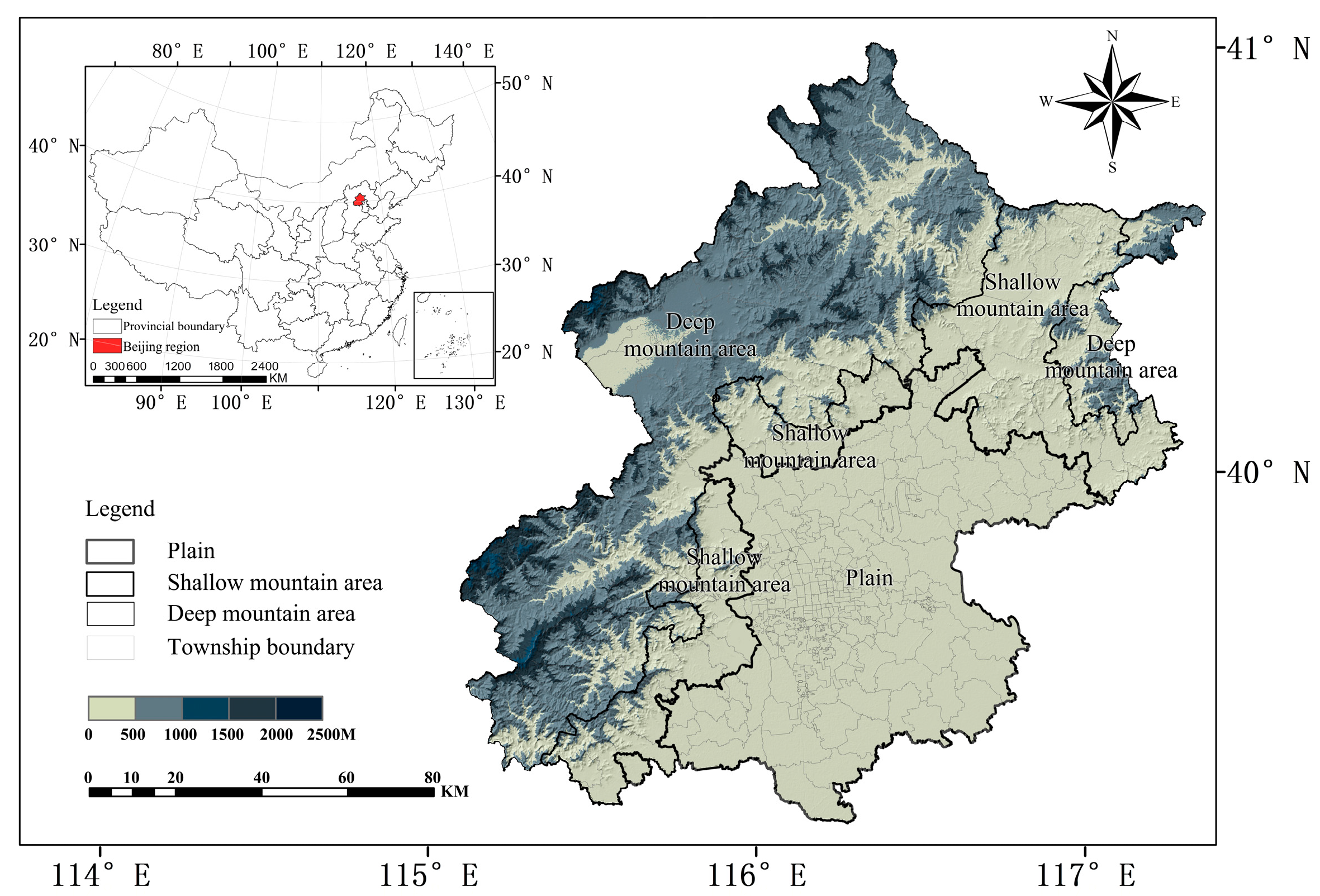
2.1. Study Area

Beijing is located in the north of China, with a total area of 16,411 km², of which the mountain area accounts for about 62% and plain areas account for about 38%. The terrain declines from the northwest mountain area to the southeast plain in a ladder pattern with various forms and levels, providing a natural platform for Beijing to build a national forest city, and this strongly promotes the rapid development of urbanization of Beijing.

Since the 1990s, the resident population of Beijing has increased at a rate of 350,000 per year; the built-up area of the city has also expanded at a rate of 13 km² per year, and the degree of urbanization has gradually spread from the plain to the mountains [41]. Today, Beijing is a megacity and one of the most typical areas with the fastest rate of urbanization in China. The Master Plan for the Coordinated Development of Beijing’s Mountain Areas (2006–2020) divides Beijing into plains, shallow mountains, and deep mountains. In this paper, with reference to previous studies, Beijing is divided into three gradients, namely the plain, shallow mountainous areas, and deep mountainous areas, the absolute altitude ranges of which are 4–75 m, 75–300 m, and 300–2300 m, respectively, taking into account the accuracy of the research and the completeness of the boundaries of administrative villages (Figure 1) [43].

2.2. Variable Selection and Data Sources

2.2.1. Variable Selection

In this study, three periods of data from 2000, 2010, and 2020 were selected to assess the urbanization level and ecosystem services in the study area.

The evaluation of the urbanization level involves many factors, such as economy, population, society, and land use [14]. Economic urbanization is represented by GDP density, population urbanization is represented by population density [40], and social urbanization is represented by social electricity consumption. In terms of land urbanization assessment, the scope of construction land in the land use data was extracted first, and the proportion of construction land was calculated to obtain the land urbanization assessment result [42]. Finally, the above results were normalized to obtain various urbanization intensities.

The type selection and calculation method of ecosystem services refer to the requirements of the Beijing Territorial Ecological Restoration Plan (2021–2035) [44] and the Guide for Delineating the Red Line of Ecological Protection (2017) [45], and four kinds of ecosystem services were selected, namely water conservation, soil and water conservation, wind prevention and sand fixation, and biodiversity protection. The net primary productivity (NPP) quantitative index evaluation method was used for calculation. Based on NPP data combined with monthly average precipitation, average temperature, average relative humidity, average wind speed, elevation, and soil data, the method can quickly and accurately assess regional ecosystem services.

A grid of the same size was used to cover the study area comprehensively for the above data. The spatial resolution of all data was uniformly adjusted to 500 m × 500 m by the ArcGis 10.8 resampling function, and the urbanization level and ecosystem services of the study area were quantitatively assessed using a raster calculator tool. Considering that previous urbanization studies take administrative districts as the basic statistical unit and China’s economic and social data take township-level administrative districts as the smallest statistical unit [41], this paper takes 331 township-level administrative districts of Beijing as the statistical unit and establishes the spatial weight matrix.

2.2.2. Data Sources

GDP and electricity consumption data from the Beijing statistics yearbook (https://nj.tjj.beijing.gov.cn/nj/main/2021-tjnj/zk/indexch.htm) (accessed on 1 November 2023); population density data from World Pop (https://hub.worldpop.org/project/categories?id=18) (accessed on 1 November 2023); land use type data from professor Yang jie, Huang Xin paper dataset (https://zenodo.org/record/5210928#.YcZ_nWBByUk) (accessed on 1 November 2023). Data from MODIS vegetation net primary productivity (https://lpdaac.usgs.gov/product_search/) (accessed on 1 November 2023), Data of monthly precipitation, average temperature, average relative humidity, and average wind speed were obtained from Data Center for Resources and Environmental Sciences, Chinese Academy of Sciences (https://www.resdc.cn) (accessed on 3 November 2023). Elevation data from Copernicus panda (https://panda.copernicus.eu/panda) (accessed on 3 November 2023), soil data from the global soil database (http://webarchive.iiasa.ac.at/Research/LUC/External-World-soil-database/HTML/HWSD_Data.html?sb=4) (accessed on 3 November 2023). Statistical and computational analysis was performed using ArcGIS 10.8 and Stata. USES Geoda 1.1.4 software to calculate weight space matrix.

2.2.3. Ecosystem Services Assessment

According to the calculation method in the Guide for Delineating the Red Line of Ecological Protection (2017) [45], the ecosystem services in the study area were evaluated by using the net primary productivity data of vegetation, monthly average precipitation, average temperature, average relative humidity, average wind speed, elevation, and soil data in 2000, 2010, and 2020. The specific quantification methods and data usage are as follows:

• Water conservation services

The ecosystem water conservation service capacity index was taken as the evaluation index, and the calculation formula is as follows [45]:

$$\mathrm{W}\mathrm{R}={\mathrm{N}\mathrm{P}\mathrm{P}}_{\mathrm{M}\mathrm{E}\mathrm{A}\mathrm{N}}\times {\mathrm{F}}_{\mathrm{s}\mathrm{i}\mathrm{c}}\times {\mathrm{F}}_{\mathrm{p}\mathrm{r}\mathrm{e}}\times (1-{\mathrm{F}}_{\mathrm{s}\mathrm{l}\mathrm{o}}),$$

(1)

where $\mathrm{W}\mathrm{R}$ is the ecosystem water conservation service ability index, ${\mathrm{N}\mathrm{P}\mathrm{P}}_{\mathrm{M}\mathrm{E}\mathrm{A}\mathrm{N}}$ is the average annual net primary productivity of vegetation, and ${\mathrm{F}}_{\mathrm{s}\mathrm{i}\mathrm{c}}$ is the soil percolating factor. ArcGIS 10.8 software is used to open the grid diagram (HWSD_China_Albers.img) in the soil dataset and connect the value field in the grid diagram attribute with the MU_GLOBAL in HWSD.mdb field (soil attribute table). The attribute value of the T_USDA_TEX field is divided by 13 to obtain the grid diagram of soil seepage factors. ${\mathrm{F}}_{\mathrm{p}\mathrm{r}\mathrm{e}}$ is the annual average precipitation factor, which is calculated from the monthly precipitation data during the study period. ${\mathrm{F}}_{\mathrm{s}\mathrm{l}\mathrm{o}}$ is the slope factor. Using the elevation dataset in the study area, the slope grid map is calculated by using the slope option in the Surface Analysis toolbox of ArcGIS 10.8 software. Finally, the above data are extracted to the study area according to the mask, and the grid calculator is used for calculation.

2.

Water and soil conservation services

The ecosystem water and soil conservation service capacity index was taken as the evaluation index, and the calculation formula is as follows [45]:

$${\mathrm{S}}_{\mathrm{p}\mathrm{r}\mathrm{o}}={\mathrm{N}\mathrm{P}\mathrm{P}}_{\mathrm{M}\mathrm{E}\mathrm{A}\mathrm{N}}\times (1-\mathrm{K})\times (1-{\mathrm{F}}_{\mathrm{s}\mathrm{l}\mathrm{o}}),$$

(2)

where ${\mathrm{S}}_{\mathrm{p}\mathrm{r}\mathrm{o}}$ is the soil and water conservation service ability index, ${\mathrm{N}\mathrm{P}\mathrm{P}}_{\mathrm{M}\mathrm{E}\mathrm{A}\mathrm{N}}$ is the average annual net primary productivity of vegetation, and ${\mathrm{F}}_{\mathrm{s}\mathrm{l}\mathrm{o}}$ is the slope factor. $\mathrm{K}$ is a soil erodibility factor, which refers to the difficulty of hydraulically separating and transporting soil particles, mainly related to soil texture, organic matter content, soil structure, permeability, and other soil physical and chemical properties. The calculation formula of $\mathrm{K}$ is as follows [45]:

$$\mathrm{K}=(-0.01383+0.51575{\mathrm{K}}_{\mathrm{E}\mathrm{P}\mathrm{I}\mathrm{C}})\times 0.1317,$$

(3)

$$\begin{gathered} {\mathrm{K}}_{\mathrm{E}\mathrm{P}\mathrm{I}\mathrm{C}}=\{0.2+0.3\exp [-0.0256{\mathrm{m}}_{\mathrm{s}}(1-{\mathrm{m}}_{\mathrm{slit}}/100)\left\}\right]\times [{\mathrm{m}}_{\mathrm{slit}}/({\mathrm{m}}_{\mathrm{c}}+{\mathrm{m}}_{\mathrm{slit}}){]}^{0.3}\times \\ \{1-0.25\mathrm{orgC}/[\mathrm{orgC}+\exp (3.72-2.95\mathrm{orgC}\left)\right]\}\times \{1-0.7(1-{\mathrm{m}}_{\mathrm{s}}/100)/ \\ \left\{\right(1-{\mathrm{m}}_{\mathrm{s}}/100)+\exp [-5.51+22.9(1-{\mathrm{m}}_{\mathrm{s}}/100)\left]\right\}\}, \end{gathered}$$

(4)

where ${\mathrm{K}}_{\mathrm{E}\mathrm{P}\mathrm{I}\mathrm{C}}$ represents soil erosibility factor before modification, and ${\mathrm{m}}_{\mathrm{c}}$, ${\mathrm{m}}_{\mathrm{s}\mathrm{l}\mathrm{i}\mathrm{t}}$, ${\mathrm{m}}_{\mathrm{s}}$, and $\mathrm{orgC}$ are silt (<0.002 mm), silt (0.002 mm~0.005 mm), sand (0.05 mm~2 mm), and the percentage content (%) of organic carbon, respectively. The above data are from the soil dataset. Finally, the above data are extracted to the study area according to the mask, and the grid calculator is used for calculation.

3.

Windproof sand fixation service

The index of ecosystem service capacity for wind prevention and sand fixation is taken as the evaluation index, and the calculation formula is as follows [45]:

$${\mathrm{S}}_{\mathrm{W}\mathrm{S}}={\mathrm{N}\mathrm{P}\mathrm{P}}_{\mathrm{M}\mathrm{E}\mathrm{A}\mathrm{N}}\times \mathrm{K}\times {\mathrm{F}}_{\mathrm{q}}\times \mathrm{D},$$

(5)

where ${\mathrm{S}}_{\mathrm{W}\mathrm{S}}$ is the service ability index of wind prevention and sand consolidation, ${\mathrm{N}\mathrm{P}\mathrm{P}}_{\mathrm{M}\mathrm{E}\mathrm{A}\mathrm{N}}$ is the average annual net primary productivity of vegetation, $\mathrm{K}$ is the soil erodibility factor, and ${\mathrm{F}}_{\mathrm{q}}$ is the average annual climatic erodivity. The formula for calculating ${\mathrm{F}}_{\mathrm{q}}$ is as follows [45]:

$${\mathrm{F}}_{\mathrm{q}}=\frac{1}{100}\sum _{\mathrm{I}=1}^{12}{\mathrm{u}}^3\left\{\frac{{\mathrm{E}\mathrm{T}\mathrm{P}}_{\mathrm{i}}-{\mathrm{P}}_{\mathrm{i}}}{{\mathrm{E}\mathrm{T}\mathrm{P}}_{\mathrm{i}}}\right\}\times \mathrm{d},$$

(6)

$${\mathrm{E}\mathrm{T}\mathrm{P}}_{\mathrm{i}}=0.19{\left(20+{\mathrm{T}}_{\mathrm{i}}\right)}^2\times (1-{\mathrm{r}}_{\mathrm{i}}),$$

(7)

$${\mathrm{u}}_2={\mathrm{u}}_1{\left({\mathrm{z}}_2/{\mathrm{z}}_1\right)}^{1/7},$$

(8)

where $\mathrm{u}$ is the monthly average wind speed at a height of 2 m, and the data source is the monthly average wind speed dataset. ${\mathrm{E}\mathrm{T}\mathrm{P}}_{\mathrm{i}}$ is the monthly potential evaporation (mm), which is calculated by Formulas (6)–(8). ${\mathrm{P}}_{\mathrm{i}}$ is monthly precipitation (mm), and the data source is the monthly average precipitation dataset. $\mathrm{d}$ is the number of days in the month, ${\mathrm{T}}_{\mathrm{i}}$ is the monthly average temperature, and the data source is the monthly average temperature dataset. ${\mathrm{r}}_{\mathrm{i}}$ is the monthly average relative humidity (%) from the monthly average relative humidity dataset. ${\mathrm{u}}_1$ and ${\mathrm{u}}_2$ indicate the wind speed at the height of ${\mathrm{z}}_1$ and ${\mathrm{z}}_2$, respectively. The data of ${\mathrm{u}}_1$ are from the monthly average wind speed dataset. The value of ${\mathrm{z}}_1$ is 2 m, and the value of ${\mathrm{z}}_2$ is 10 m.

$\mathrm{D}$ is the surface roughness factor, and $\mathsf{\theta }$ is the slope (radian). Based on the slope grid diagram, the grid calculator tool is used in ArcGis 10.8 software to determine $\mathrm{D}$, the calculation formula of which is as follows [45]:

$$\mathrm{D}=1/\cos \left(\mathsf{\theta }\right),$$

(9)

Finally, the above data are extracted to the study area according to the mask, and the grid calculator is used for calculation.

4.

Biodiversity conservation services

The ecosystem biodiversity maintenance service capacity index was taken as the assessment index, and the calculation formula is as follows [45]:

$${\mathrm{S}}_{\mathrm{b}\mathrm{i}\mathrm{o}}={\mathrm{N}\mathrm{P}\mathrm{P}}_{\mathrm{M}\mathrm{E}\mathrm{A}\mathrm{N}}\times {\mathrm{F}}_{\mathrm{p}\mathrm{r}\mathrm{e}}\times {\mathrm{F}}_{\mathrm{t}\mathrm{e}\mathrm{m}}\times (1-{\mathrm{F}}_{\mathrm{a}\mathrm{l}\mathrm{t}})$$

(10)

where ${\mathrm{S}}_{\mathrm{b}\mathrm{i}\mathrm{o}}$ is the biodiversity maintenance service index, ${\mathrm{N}\mathrm{P}\mathrm{P}}_{\mathrm{M}\mathrm{E}\mathrm{A}\mathrm{N}}$ is the average annual net primary productivity of vegetation, and ${\mathrm{F}}_{\mathrm{p}\mathrm{r}\mathrm{e}}$ is the average annual precipitation factor, which is calculated from the monthly average precipitation. ${\mathrm{F}}_{\mathrm{t}\mathrm{e}\mathrm{m}}$ is the annual average temperature, which is calculated from the monthly average temperature. ${\mathrm{F}}_{\mathrm{a}\mathrm{l}\mathrm{t}}$ is the elevation factor, and the data source is the elevation dataset.

According to the deviation standardization method, the results of the above ecosystem services evaluations were unified into the 0–1 range; finally, the calculated results for each service were added with equal weights to obtain integrated ecosystem services.

2.2.4. Statistical Method

• Correlation analysis

Spatial autocorrelation analysis is the core method to accurately identify the interdependence of different variable data in the same distribution region. Global Moran’s I and local Moran’s I were used in this study to measure and test the spatial attributes of ecosystem services in the study area. The calculation formula is as follows:

(1)

Global Moran’s I

Global Moran’s I can indicate whether the distribution of regional attribute values is clustered, discrete, or random. The range of global Moran’s I is [−1, 1]. When global Moran’s I is greater than 0, it indicates that the data present a positive spatial correlation, and the larger the value, the more obvious the spatial correlation. When global Moran’s I is less than 0, it means that the data present negative spatial correlation, and the smaller the value, the greater the spatial difference. When global Moran’s I is 0, the space is random. The global Moran index is calculated as follows:

$$\mathrm{G}\mathrm{o}\mathrm{l}\mathrm{a}\mathrm{l} \mathrm{M}\mathrm{o}\mathrm{r}\mathrm{a}\mathrm{n}’\mathrm{s} \mathrm{I}=\frac{\mathrm{n}}{{\sum }_{\mathrm{i}=1}^{\mathrm{n}}{\sum }_{\mathrm{j}=1}^{\mathrm{n}}{\mathrm{W}}_{\mathrm{i}\mathrm{j}}}\times \frac{{\sum }_{\mathrm{i}=1}^{\mathrm{n}}{\sum }_{\mathrm{j}=1}^{\mathrm{n}}{\mathrm{W}}_{\mathrm{i}\mathrm{j}}({\mathrm{x}}_{\mathrm{i}}-\overline{\mathrm{x}})({\mathrm{x}}_{\mathrm{j}}-\overline{\mathrm{x}})}{{\sum }_{\mathrm{i}=1}^{\mathrm{n}}{({\mathrm{x}}_{\mathrm{i}}-\overline{\mathrm{x}})}^2},$$

(11)

where $\mathrm{n}$ is the number of space units; ${\mathrm{x}}_{\mathrm{i}}$ and ${\mathrm{x}}_{\mathrm{j}}$ are the observed values of unit i and unit j, respectively; and ${\mathrm{W}}_{\mathrm{i}\mathrm{j}}$ is the spatial weight adjacency matrix of units i and j (i, j = 1, 2, 3, …, n).

(2)

Local Moran’s I

Local Moran’s I is used to reveal spatial clusters and outliers in a specific region, and when global Moran’s I shows the presence of spatial autocorrelation, local Moran’s I can help determine the specific location where this autocorrelation occurs. The local Moran index is calculated as follows:

$$\mathrm{L}\mathrm{o}\mathrm{c}\mathrm{a}\mathrm{l} \mathrm{M}\mathrm{o}\mathrm{r}\mathrm{a}\mathrm{n}’\mathrm{s} \mathrm{I}=\frac{{\mathrm{x}}_{\mathrm{i}}-\overline{\mathrm{x}}}{\frac{{\sum }_{\mathrm{i}=1,\mathrm{j}\ne 1}^{\mathrm{n}}{\mathrm{W}}_{\mathrm{i}\mathrm{j}}}{\mathrm{n}-1}-{\overline{\mathrm{x}}}^2}\times \sum _{\mathrm{j}=1,\mathrm{j}\ne 1}^{\mathrm{N}}{\mathrm{W}}_{\mathrm{i}\mathrm{j}}\left({\mathrm{x}}_{\mathrm{i}}-\overline{\mathrm{x}}\right)$$

(12)

where $\mathrm{n}$ is the number of space units, ${\mathrm{x}}_{\mathrm{i}}$ is the observed value of unit I, and ${\mathrm{W}}_{\mathrm{i}\mathrm{j}}$ is the spatial weight adjacency matrix of units i and j (i, j = 1, 2, 3, …, n).

2.

Regression model

(1)

Ordinary least square (OLS) model

OLS is a statistical method used to estimate the relationship between a dependent variable and one or more independent variables. It is widely used in regression analyses. The goal of the OLS model is to minimize the sum of squared variances between the observed and predicted values. The formula of the OLS model can be expressed as follows:

$$\mathsf{\gamma }={\mathsf{\beta }}_0+{\mathsf{\beta }}_1{\mathrm{X}}_1+{\mathsf{\beta }}_2{\mathrm{X}}_2+\cdots +{\mathsf{\beta }}_{\mathrm{n}}{\mathrm{X}}_{\mathrm{n}}+\mathsf{\epsilon }$$

(13)

where $\mathsf{\gamma }$ is the dependent variable; ${\mathrm{X}}_1$, ${\mathrm{X}}_2$, …, and ${\mathrm{X}}_{\mathrm{n}}$ are the independent variables; ${\mathsf{\beta }}_0$, ${\mathsf{\beta }}_1$, ${\mathsf{\beta }}_2$, …, and ${\mathsf{\beta }}_{\mathrm{n}}$ are the coefficients representing the relationship between the dependent andindependent variables; and $\epsilon$ is the error term representing the unexplained variation in the dependent variable.

(2)

Spatial weight matrix

A spatial weight matrix of the study area [331, 331] was constructed using the first law of geography, which indicates that the relationship between geographical regions weakens with the increase in geographical distance. A binary space weight matrix was constructed using Geoda 1.14 software, then converted into a standard 331 × 331 space weight matrix by Stata 17. To explore the law of elevation differentiation, the corresponding spatial weight matrix was generated according to the elevation gradient partitions of the plain area, shallow mountain area, and deep mountain area. The expression of the spatial weight matrix is as follows:

$$\begin{array}{cc}\mathrm{w}=& \left[\begin{array}{cccccc}{\mathrm{w}}_{11}& {\mathrm{w}}_{12}& .& .& .& {\mathrm{w}}_{1\mathrm{n}}\\ {\mathrm{w}}_{21}& {\mathrm{w}}_{22}& .& .& .& {\mathrm{w}}_{2\mathrm{n}}\\ .& .& & & & .\\ .& .& & & & .\\ .& .& & & & .\\ {\mathrm{w}}_{\mathrm{n}1}& {\mathrm{w}}_{\mathrm{n}2}& .& .& .& {\mathrm{w}}_{\mathrm{n}\mathrm{n}}\end{array}\right]\end{array},$$

(14)

(3)

Spatial econometric model

The spatial econometric model is a statistical model used to analyze spatial correlation and dependence. It captures the mutual influence and dependence between adjacent regions of geographic space by incorporating spatial factors and reflects the degree of mutual influence of geographic space. The matrix includes endogenous interaction (WY) and exogenous interaction (WX). The most commonly used spatial measurement models include the spatial Durbin model (SDM), spatial lag model (SLM), and spatial error model (SEM).

The spatial Durbin model (SDM) includes both WY and WX interaction effects, expressed as follows:

$$\mathsf{\gamma }=\mathsf{\rho }\mathrm{W}\mathsf{\gamma }+\mathrm{X}\mathsf{\beta }+\mathrm{W}\mathrm{X}\mathsf{\theta }+\mathsf{\epsilon },\mathsf{\epsilon }~\mathrm{N}\left(0,{\mathsf{\delta }}^2\right),$$

(15)

where $\mathsf{\gamma }$ is the dependent variable, $\mathrm{W}$ is the spatial weight matrix that captures the spatial correlation between sample elements, $\mathrm{X}$ is the independent variable matrix, $\mathsf{\beta }$ is the coefficient vector of the independent variable, $\mathsf{\theta }$ is the coefficient of the exogenous interaction effect, $\mathrm{W}\mathrm{X}$ is the spatial lag-independent variable matrix, and $\mathsf{\epsilon }$ is the error term. Suppose $\mathsf{\epsilon }$ follows a multivariate normal distribution with a mean of zero and a constant scalar diagonal variance–covariance matrix (${\mathsf{\delta }}^2$). When $\mathsf{\theta }$ = 0, it corresponds to the SLM. When $\mathsf{\theta }$ = −$\mathsf{\rho }\mathsf{\beta }$, it corresponds to the SEM. When the error term of the model has a spatial correlation, it is called the SLM and expressed as follows:

$$\mathsf{\gamma }=\mathsf{\rho }\mathrm{W}\mathsf{\gamma }+\mathrm{X}\mathsf{\beta }+\mathsf{\epsilon },\mathsf{\epsilon }~\mathrm{N}\left(0,{\mathsf{\delta }}^2\right),$$

(16)

When spatial dependence between dependent variables leads to spatial correlation in the model, it is called a spatial error model, also known as an SEM, and is expressed as follows:

$$\mathsf{\gamma }=\mathrm{X}\mathsf{\beta }+\mathsf{\lambda }{\mathrm{W}}_{\mathrm{u}}+\mathsf{\epsilon },\mathsf{\epsilon }~\mathrm{N}\left(0,{\mathsf{\delta }}^2\right),$$

(17)

where $\mathrm{u}$ is the random error vector, and $\mathsf{\lambda }$ is the spatial correlation coefficient between the regression residuals [46].

3. Results

3.1. Temporal and Spatial Characteristics of Urbanization Level

It can be seen from Figure 2 that from 2000 to 2020, the high-value area of urbanization in the study area was concentrated in the middle of the plain and continuously expanded outward. This area is flat, can easily access various resources, and is suitable for large-scale construction activities. The low-value area was concentrated in the deep mountainous area and the northern shallow mountainous area. The terrain of this area is mainly mountainous, and the activities of production and life are greatly restricted here [32,41].

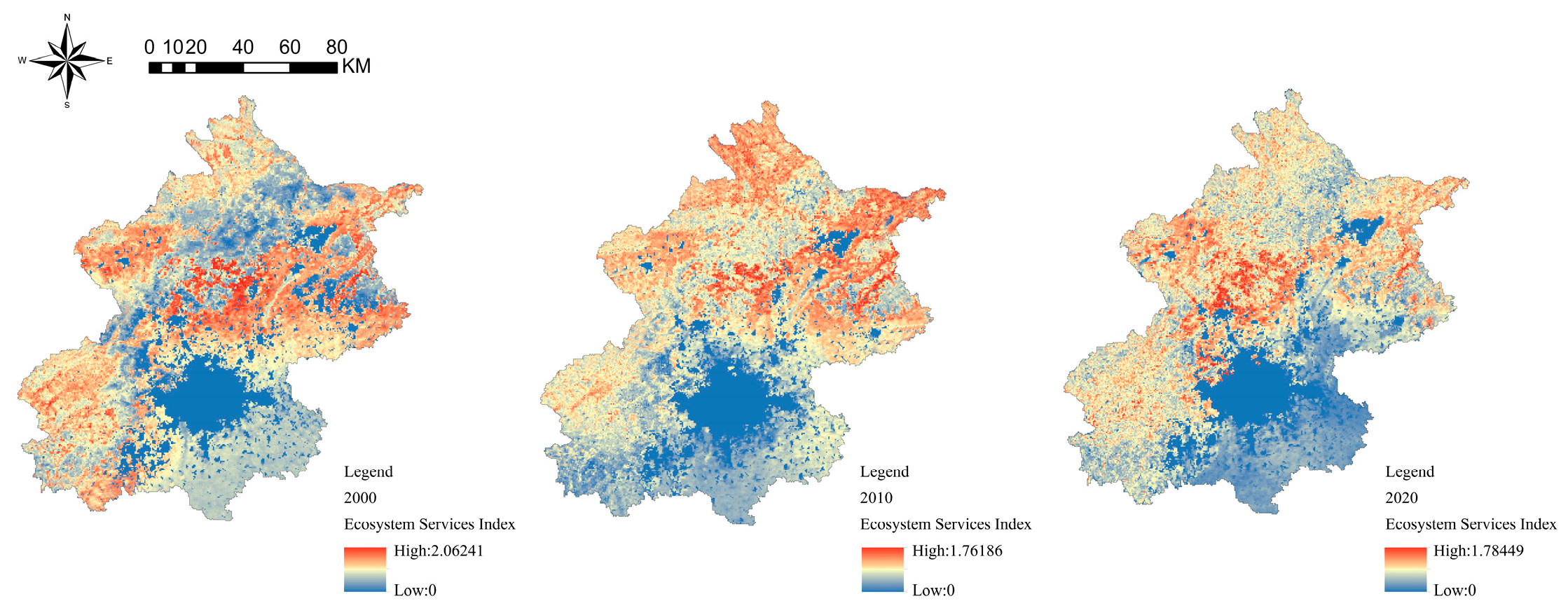
3.2. Temporal and Spatial Characteristics of Ecosystem Services

The results of the study (Figure 3) show that the ecosystem service index decreased first, then increased, with the high-value area concentrated in the shallow and deep mountains in the northwest and the low-value area concentrated in the southeastern plain. During the rapid development of urbanization from 2000 to 2010, the ecosystem service index decreased from 2.06241 to 1.76186. From 2010 to 2020, with the development of ecological environment projects such as returning farmland to forest, the ecosystem service function index recovered to 1.78449.

3.3. Autocorrelation Analysis of Ecosystem Services

Before applying the spatial econometric model, it is necessary to detect the spatial autocorrelation of ecosystem services in the study area. In Arcgis10.8 software, the final results of ecosystem service assessment were counted for 331 township-level administrative districts using the spatial weight matrix constructed above and based on stata 17 software. Spatial autocorrelation of ecosystem services in the study area was analyzed using global and local Moran’s I statistics.

As can be seen from

Table 1. Results of global Moran’s I regression.

Variables	I	E(I)	Sd(I)	z	p-Value
2000 ecosystem services	0.829	−0.003	0.033	25.087	0.000 ***
2010 ecosystem services	0.877	−0.003	0.033	26.536	0.000 ***
2020 ecosystem services	0.850	−0.003	0.033	25.720	0.000 ***

*, **, and *** indicate the significance levels at 10%, 5%, and 1%, respectively.

, the global Moran’s I values in 2000, 2010, and 2020 are 0.829, 0.877, and 0.850, respectively, indicating that there is a positive spatial autocorrelation of ecosystem services during the entire observation period. The ecosystem services in adjacent areas have certain spatial dependence and local clustering distribution characteristics. The p-values in the detection results are all 0.000, indicating that the detection results are significant at a 1% confidence level.

To further understand the spatial agglomeration characteristics and local spatial correlations of ecosystem services, the local Moran’s I was calculated, and local Moran’s I scatter plots were plotted for 2000, 2010, and 2020. As can be seen from Figure 4, the local Moran’s I scatter plot shows that ecosystem services present a high–high (H-H) or low–low (L-L) spatial distribution pattern, which indicates that ecosystem services in the study area present a strong clustering and that the spatial pattern of local clustering has been relatively stable. The above results indicate that further analysis with a regression model is needed.

3.4. Regression Result of Ordinary Least Square (OLS) Method

The influence relationship between urbanization and ecosystem services was analyzed by ordinary least square regression (

Table 2. Regression results of OLS model.

	Plain			Shallow Mountain Area			Deep Mountain Area
	Ind	Time	Spatiotemporal	Ind	Time	Spatiotemporal	Ind	Time	Spatiotemporal
Main
Economic urbanization	0.028	−0.091 ***	0.031 *	0.006	−0.013	−0.006	−0.032	−0.079 ***	−0.069 *
	(1.56)	(−6.11)	(1.71)	(0.83)	(−1.51)	(−0.72)	(−0.90)	(−2.72)	(−1.83)
Population urbanization	−0.096 ***	−0.005	0.016	−0.044 *	−0.043 **	−0.020	0.272 ***	0.039	0.143
	(−2.83)	(−0.17)	(0.22)	(−1.81)	(−2.48)	(−0.78)	(2.79)	(0.63)	(1.41)
Social urbanization	0.002	−0.003 **	0.003 **	0.031	−0.069 *	−0.014	0.116	−0.009	−0.098
	(1.41)	(−2.53)	(2.23)	(0.66)	(−1.74)	(−0.14)	(1.22)	(−0.28)	(−0.78)
Land urbanization	−0.290 ***	−0.240 ***	−0.370 ***	−0.008 ***	−0.011 ***	−0.008 ***	−0.016 *	−0.016 ***	−0.017 **
	(−4.93)	(−3.93)	(−4.97)	(−3.26)	(−6.78)	(−3.19)	(−1.98)	(−5.21)	(−2.17)
r2	0.433	0.445	0.440	0.083	0.126	0.113	0.156	0.266	0.201

*, **, and *** indicate the significance levels at 10%, 5%, and 1%, respectively.

). Since OLS regression alone may produce certain deviations when estimating the impacts of explanatory variables on ecosystem services, the spatial econometric model was applied for further testing, and the regression model with the best fit was selected by comparing the results of the two.

3.5. Estimation of Spatial Econometric Model

3.5.1. Selective Testing of Spatial Econometric Models

Before using the spatial econometrics model, it is necessary to select the most appropriate measurement model according to the test decision rules. First, the LM test and robustness test were combined to determine whether there were spatial error effects and spatial lag effects. Secondly, the WALD and LR tests were used to determine whether the spatial Durbin model (SDM) could be degenerated into a spatial lag model (SLM) and spatial error model (SEM), that is, to determine the applicability of the SDM model. If it could not be degraded, the SDM model with a spatial lag term and a spatial error term was used; otherwise, the degraded model was selected. From the results shown in

Table 3. LM, LR, WALD, and Hausman testing.

	Methods	z	p-Value
LM Test	LM–spatial lag	644.848	0.000
	Robust LM–spatial lag	269.604	0.000
	LM–spatial error	454.075	0.000
	Robust LM–spatial error	78.831	0.000
Wald Test	Wald–spatial lag	53.42	0.000
	LR–spatial lag	49.96	0.000
	Wald–spatial error	23.52	0.009
	LR–spatial error	18.88	0.004
Hausman Test	Assumption is nested within both	4.29	1.000
	Assumption time nested within both	2423.42	0.000

, we can infer that the statistics of LM and the robustness test were significant, indicating that both the SLM and SEM models were applicable, and the SDM model was initially selected. Subsequently, the results of the WALD and LR tests were rejected under the original hypothesis of SDM model degradation and passed the 1% significance test, so we decided to use the SDM model for regression analysis. Combined with the Hausman test (Table 3), the time-fixed effect model as part of the SDM model was selected [46].

3.5.2. Regression Results of Spatial Durbin Model

The spatially fixed effect and time-fixed effect of the SDM model were used to compare the regression results. It can be seen from

Table 4. Regression results of SDM model.

	Plain			Shallow Mountain Area			Deep Mountain Area
	Ind	Time	Spatiotemporal	Ind	Time	Spatiotemporal	Ind	Time	Spatiotemporal
Main
Economic urbanization	−0.105 ***	−0.150 **	−0.130 ***	−0.135 *	−0.138 **	0.136 *	0.279 ***	−0.052 ***	0.272 ***
	(−3.71)	(−2.36)	(−4.49)	(−1.90)	(−2.04)	(1.89)	(4.79)	(−2.77)	(4.76)
Population urbanization	0.006	−0.052 ***	0.030	−0.136 **	−0.035	−0.138 **	−0.030	−0.001	−0.088
	(0.16)	(−2.82)	(0.76)	(−2.34)	(−0.98)	(−2.28)	(−0.61)	(−0.01)	(−1.54)
Social urbanization	−0.031 ***	−0.030	−0.030 ***	0.004	−0.056	0.005	−0.012	−0.022	0.060
	(−2.70)	(−1.30)	(−2.61)	(0.14)	(−1.40)	(0.19)	(−0.19)	(−0.48)	(0.97)
Land urbanization	−0.002 ***	−0.007 ***	−0.002 **	−0.013 ***	−0.013 ***	−0.013 ***	−0.018 ***	−0.010 ***	−0.021 ***
	(−3.16)	(−6.08)	(−2.54)	(−7.76)	(−9.26)	(−7.74)	(−4.32)	(−5.16)	(−5.05)
Wx
Economic urbanization	0.018	−0.070 ***	−0.113 **	−0.090	−0.002	−0.092	−0.316 ***	−0.026	−0.391 ***
	(0.42)	(−5.33)	(−2.00)	(−0.91)	(−0.03)	(−0.83)	(−3.91)	(−0.86)	(−4.35)
Population urbanization	−0.019	−0.003	0.105 **	0.135 **	−0.044	0.118	0.158 **	−0.021	0.079
	(−0.47)	(−0.13)	(1.97)	(2.15)	(−0.99)	(1.45)	(2.19)	(−0.35)	(0.82)
Social urbanization	0.046 ***	0.089 ***	0.051 ***	−0.021	−0.046	−0.016	0.091	0.095 ***	−0.051
	(2.91)	(2.99)	(3.24)	(−0.67)	(1.04)	(−0.49)	(1.22)	(3.08)	(−0.59)
Land urbanization	0.004 ***	−0. 900 ***	0.006 ***	0.011 ***	0.008	0.011 ***	−0.002	−0.003	0.006
	(4.15)	(−4.98)	(5.47)	(4.65)	(−0.72)	(4.38)	(−0.17)	(−0.45)	(0.45)
Spatial rho	0.880 ***	0.805 ***	0.870 ***	0.752 ***	0.593 ***	0.747 ***	0.742 ***	0.655 ***	0.727 ***
	(47.35)	(28.93)	(45.27)	(24.30)	(12.81)	(23.64)	(16.69)	(7.22)	(15.71)
r2	0.012	0.792	0.382	0.773	0.781	0.764	0.352	0.423	0.423

*, **, and ***, respectively, indicate the significance levels at 10%, 5%, and 1%.

that the spatial Durbin model ($R^2$) of the time-fixed effect was the largest and produced the most significant results. Combined with the Hausman test, as shown above, the SDM model of the time-fixed effect was selected for regression analysis and effect decomposition. At the same time, the spatial autoregressive coefficient spatial rho was significant and positive, indicating that there was a significant positive spatial spillover effect of neighboring ecosystem services, that is, the improvement of neighboring ecosystem services is conducive to the improvement of local ecosystem services. The regression results of the explanatory variables are different in the three regions, which proves that there are altitude differences in the impacts of urbanization on ecosystem services.

3.5.3. Direct Effect and Indirect Effect Analysis

The regression results of the decomposed spatial Durbin model are shown in

Table 5. Results showing direct and indirect effects of urbanization on ecosystem services under altitude gradient.

		Economic Urbanization	Population Urbanization	Social Urbanization	Land Urbanization
Main
Direct effects	Plain	−0.006 ***	−0.040 *	0.033	−0.220 ***
		(−4.95)	(−1.89)	(1.56)	(−3.38)
	Shallow mountain area	−0.013 ***	−0.055	−0.047	−0.152 **
		(−9.01)	(−1.51)	(−1.42)	(−2.24)
	Deep mountain area	−0.013 ***	−0.036	−0.032	−0.054 **
		(−4.28)	(−0.71)	(−1.42)	(−2.34)
Indirect effects	Plain	−0.015 **	−0.131 *	0.428 ***	−0.935 **
		(−2.26)	(−1.90)	(4.25)	(−2.56)
	Shallow mountain area	−0.001	0.029	−0.151 **	−0.186
		(−0.08)	(0.54)	(−1.99)	(−1.35)
	Deep mountain area	−0.025	−0.097	0.153 *	−0.026
		(−1.29)	(−0.64)	(1.76)	(−0.29)
Total effects	Plain	−0.021 **	−0.171 **	0.461 ***	−1.155 ***
		(−2.30)	(−2.49)	(4.37)	(−2.98)
	Shallow mountain area	−0.014 ***	−0.026	−0.198 **	−0.338 **
		(−4.32)	(−0.60)	(−2.44)	(−2.01)
	Deep mountain area	−0.038 *	−0.133	0.121	−0.081
		(−1.74)	(−0.75)	(1.17)	(−0.75)

*, **, and *** indicate the significance levels at 10%, 5%, and 1%, respectively.

.

In the plain area, the direct and indirect effects of economic, population, and land urbanization were all negative, which means that the three forms of urbanization have a significant negative impact on local ecosystem services, and the absolute value of the indirect effect is greater than that of the direct effect. The results show that the spatial spillover effects of urbanization have more negative effects on the surrounding ecosystem services. The direct effect of social urbanization is not statistically significant, meaning that its impact on local ecosystem services is not significant. However, the regression coefficients for both indirect and total effects are positive, suggesting that social urbanization in adjacent areas has a significant positive impact on ecosystem services locally and across the plains.

In shallow mountainous areas, the direct and total effects of economic urbanization and land urbanization are negative, and the indirect effects failed to pass the significance test, which indicates that economic urbanization and land urbanization mainly have negative impacts on local ecosystem service functions in shallow mountainous areas. The indirect and total effects of social urbanization are negative, while the direct effects are not significant, indicating that in shallow mountainous areas, social urbanization in neighboring areas has a negative impact on local ecosystem services.

In deep mountain areas, the effects of economic urbanization and land urbanization were found to be the same as in the shallow mountains. The indirect effect of social urbanization is positive, but the direct effect is not significant, which indicates that in deep mountainous areas, the social urbanization of neighboring areas has a positive impact on the local ecosystem service function.

4. Discussion

4.1. Comparative Analysis of the Results

During the study period, affected by the distribution of resources, the intensity of human activities and the difficulty of development, the high-value area of urbanization in Beijing was concentrated in the middle of the plain [40]. The high value of the ecosystem service index was found to be concentrated in shallow and deep mountainous areas, which may be due to the influence of ecological environment construction projects such as returning farmland to forest. Since 2002, Beijing has returned a total of 700 km² of farmland to forest, reducing the rate of soil and water loss in shallow and deep mountain slopes and sandy wasteland, reducing the damage of wind and sand, and maintaining a high level of ecosystem services [47]. The Moran’s I results show that the spatial distribution of ecosystem services in Beijing could be characterized as low–low agglomeration or high–high agglomeration, with significant spatial autocorrelation. Compared with previous studies, this paper considers the direct impact of urbanization on ecosystem services and the spatial spillover effect under altitude gradients.

4.1.1. Impacts of Urbanization on Ecosystem Services in Plain Areas

In plain areas, economic, population and land urbanization were found to have negative impacts on local and adjacent ecosystem services, particularly on neighboring areas (Figure 5). The reason is that the plain area is relatively rich in resources that are easy to obtain, population and industrial agglomeration lead to the excessive consumption of resources and environmental damage, and the large-scale expansion of construction land undermines the stability of the original regional ecosystem, having a negative impact on ecosystem services. This is consistent with the results obtained by Zhang et al. using the pressure—state–response (PSR) framework [25]. In addition, the ecosystem service index in the plain area showed a spatial distribution of low in the middle and high in the periphery, and the ecosystem type in the plain area was relatively simple, while the regional self-regulation ability and the ability to resist human disturbance were poor. This is consistent with the findings of Wang et al. [48]. Therefore, the development of economy, population, and land urbanization will have a greater impact on the ecosystem service function of neighboring areas, which highlights the importance of the coordinated development of regional urbanization. It reflects the scientificity of the requirement of overall planning in Beijing’s territorial space planning. In contrast, social urbanization has a positive impact on ecosystem services in neighboring areas. The reason may be that, in the context of high-quality development, Beijing vigorously supports the development of high-tech industries and green-energy industries, and the levels of technological innovation and environmental protection awareness have increased. Social urbanization has promoted the improvement of talent quality and the upgrading of surrounding industries, and energy utilization has attained high efficiency and scale. This transformation will help reduce the impacts of human activities on the natural environment and establish a win–win situation between economic development and ecological protection. A large number of studies have supported this view from different perspectives, such as low-carbon economy and green finance [49,50,51,52]. Thus, the positive effects of high-quality social urbanization on ecosystem services, combined with changes in people’s values and lifestyles, are likely to have lasting positive effects [53].

4.1.2. Impacts of Urbanization on Ecosystem Services in Shallow and Deep Mountain Areas

In shallow and deep mountain areas, economic urbanization and land urbanization have negative impacts on local ecosystem services, especially in deep mountain areas (Figure 5). On the one hand, enterprises or industries characterized by high pollution and energy consumption have a serious impact on the quality of local air, water, and soil, and the function of ecosystem services is thus reduced. On the other hand, land urbanization has promoted the conversion of the original large area of forest land to construction land, resulting in soil erosion, vegetation destruction and other problems. The relatively high costs of land development and utilization in shallow and deep mountain areas have further expanded the negative impacts of urbanization, and deep mountain areas with low urbanization levels are more affected by this process. This is consistent with the results obtained by Xie et al. [28] by assessing the spatio-temporal changes in the value of ecosystem services in mountain areas, finding that mountainous areas with higher ecological environmental quality are more likely to be affected by construction activities. To date, a large number of studies, taking Beijing as a research area, have obtained the same views from the perspectives of the social–ecosystem vulnerability relationship in mountain areas and the ecological vulnerability of mountain forests [54,55,56,57]. The impacts of social urbanization on ecosystem services in shallow and deep mountain areas are different, which may be a result of different driving factors. In shallow mountain areas, social urbanization has a negative impact on ecosystem services in neighboring areas. This is related to the low quality of social urbanization development in shallow mountain areas and the relatively fragile ecological environment. For example, the overdevelopment of scenic spots and an influx of industrial enterprises may cause damage to the ecological environment. In deep mountain areas, social urbanization has a positive impact on the ecosystem services of neighboring areas. The reason may be that social urbanization in the deep mountains is mainly driven by the construction of ecological environmental engineering and ecological tourism projects [57,58]. In addition, the ecosystem in the deep mountains is relatively complete and has a strong self-repair ability and stability, meaning it can resist the negative impact of social urbanization to a certain extent. Moderate and reasonable development and utilization may help to protect and restore the ecosystem here. In Chen et al.’s study, the FLUS model coupled with a Markov chain was used to predict the ecosystem service level of the ecological conservation area in northwest Beijing in 2030 under the scenarios of natural evolution, ecological control, and rapid urban development, among which the ecosystem service function was the best under the ecological control scenario. This supports the viewpoint of this paper to some extent [59].

Compared with plain areas, the natural conditions of shallow mountain areas and deep mountain areas are more complex. Affected by the natural characteristics of mountain areas, such as surface fragmentation, energy hierarchy, and spatial heterogeneity, these are often the key areas showing unbalanced and inadequate development. We see here an array of nature–human interaction and coupling characteristics, such as the vulnerability of the ecosystem, the tightness of geographical space, and the marginality of social economy. This limits large-scale urbanization [60]. Therefore, in shallow and deep mountain areas, the impacts of population urbanization are not obvious; similarly, the spillover effects of economic urbanization and land urbanization are not significant.

From the above discussion, it can be inferred that ignoring the difference in the impact of urbanization on ecosystem services at different altitudes may reduce the explanatory power of the research conclusions as regards the actual situation. The regression results of the spatial Durbin model indicate the importance of altitude factors in exploring the impact of urbanization on ecosystem services, as well as the necessity and scientific nature of regional coordinated and benign development, which indirectly reflects the rationality of using the spatial Durbin model for estimation in this paper. However, the specific quantitative relationship and mechanism of action still need a lot of empirical results to prove.

4.2. Discussion of Models

Based on dynamic panel data, this paper has used the spatial Durbin model with time-fixed effects to carry out regression. Since the dynamic panel data feature both cross-sectional latitude (n-bit individuals) and time–latitude (T periods), the sample size is larger, meaning it can provide more information about the dynamic behavior of individuals and solve the problem of missing variables caused by unobserved individual differences or “heterogeneity”. The results can thus be estimated more accurately [37].

The spatial Durbin model of fixed effects holds that explanatory variables can be correlated with individual characteristic variables, while the random effects model takes individual characteristic variables into the random error term, that is, it assumes that explanatory variables cannot be correlated with individual characteristic changes, and the required conditions are more ideal than those of fixed effects. Therefore, the fixed-effect model has more parameters to be estimated, and the degree of freedom of the model is more strictly controlled, which can reduce the error caused by missing variables. In empirical studies undertaken using the spatial Durbin model, most scholars choose fixed effects [36,44,61].

Time-fixed effects can solve the problem of variables that change over time being missing from the estimation process and compare the differences between regions based on the performances of each over multiple time periods. Individual fixation is used to capture differences between individuals that do not change over time, such as gender, or characteristic variables such as job and school over time. This study focuses on the impact of urbanization on ecosystem service function. The explanatory variables of each study sample vary greatly in different periods, which is more consistent with the characteristics of time-fixed effects [39].

According to the regression results, the relationship between urbanization and ecosystem services under altitude gradient is partially consistent with the results of the SEM (

Table 6. Regression results of SLM model.

	Plain			Shallow Mountain Area			Deep Mountain Area
	Ind	Time	Spatiotemporal	Ind	Time	Spatiotemporal	Ind	Time	Spatiotemporal
Main
Economic urbanization	−0.002	−0.014	−0.001	−0.000	−0.020	−0.008 *	−0.003	−0.006	−0.010
	(−1.00)	(−1.62)	(−0.22)	(−0.08)	(−1.39)	(−1.66)	(−0.18)	(−0.26)	(−0.56)
Population urbanization	0.002	0.013	0.003	−0.013	0.004	−0.005	0.054	−0.027	0.036
	(0.26)	(1.12)	(0.45)	(−1.04)	(0.24)	(−0.35)	(1.18)	(−0.68)	(0.78)
Social urbanization	0.048 ***	0.098 ***	0.087 ***	0.052 **	−0.022	−0.029	−0.027	−0.035 *	−0.033
	(3.37)	(5.70)	(3.05)	(2.12)	(−0.77)	(−0.56)	(−0.62)	(−1.96)	(−0.58)
Land urbanization	0.001	−0.003 ***	0.001 **	−0.007 ***	−0.008 ***	−0.008 ***	−0.008 **	−0.011 ***	−0.013 ***
	(1.43)	(−3.09)	(2.09)	(−5.47)	(−6.61)	(−5.73)	(−2.26)	(−6.61)	(−3.60)
Spatial rho	0.836 ***	0.663 ***	0.833 ***	0.722 ***	0.390 ***	0.718 ***	0.753 ***	0.730 ***	0.755 ***
	(41.45)	(22.19)	(41.08)	(21.69)	(8.42)	(21.34)	(17.59)	(11.37)	(17.17)
r2	0.743	0.761	0.119	0.632	0.757	0.719	0.224	0.084	0.232

*, **, and *** indicate the significance levels at 10%, 5%, and 1%, respectively.

) and SLM (

Table 7. Regression results of SEM model.

	Plain			Shallow Mountain Area			Deep Mountain Area
	Ind	Time	Spatiotemporal	Ind	Time	Spatiotemporal	Ind	Time	Spatiotemporal
Main
Economic urbanization	0.009	−0.001	0.009	0.006	−0.009	−0.017	0.073 ***	0.076	0.004
	(1.44)	(−0.05)	(1.33)	(0.72)	(−0.37)	(−1.62)	(2.65)	(1.39)	(0.10)
Population urbanization	−0.026 **	−0.044 **	−0.026 **	−0.010	−0.026	0.005	0.006	−0.026	0.058
	(−2.33)	(−2.22)	(−2.32)	(−0.41)	(−0.98)	(0.21)	(0.10)	(−0.50)	(0.97)
Social urbanization	−0.016	0.015	−0.016	−0.014	−0.068 **	−0.144 **	−0.044	−0.050 ***	−0.097 *
	(−0.49)	(0.69)	(−0.42)	(−0.33)	(−2.07)	(−2.40)	(−0.93)	(−2.88)	(−1.86)
Land urbanization	−0.002 ***	−0.007 ***	−0.002 ***	−0.012 ***	−0.014 ***	−0.013 ***	−0.017 ***	−0.012 ***	−0.014 ***
	(−2.98)	(−6.14)	(−2.98)	(−7.24)	(−10.78)	(−7.80)	(−4.22)	(−7.30)	(−3.92)
Spatial rho	0.896 ***	0.853 ***	0.895 ***	0.765 ***	0.607 ***	0.757 ***	0.802 ***	0.781 ***	0.777 ***
	(52.80)	(35.65)	(52.11)	(24.17)	(13.02)	(24.77)	(22.84)	(12.94)	(19.95)
r2	0.758	0.771	0.758	0.397	0.761	0.643	0.063	0.181	0.094

*, **, and *** indicate the significance levels at 10%, 5%, and 1%, respectively.

). However, the degrees of fit of both are inferior to that of the SDM, which confirms the robustness of the LR, Wald, and Hausman tests shown in Section 3.5.1 and justifies the use of the SDM.

Based on the above discussion and analysis, we can see that the spatial Durbin model of time-fixed effects is superior to other models.

4.3. Future Construction Proposal

Future urban development and construction should, on the one hand, be approached via the aspects of land use, industrial structure, ecological carrying capacity, and so on. In plain areas, the development goal is to build a sustainable city with “resource conservation, environmental friendliness, regional coordination and ecological low carbon”, reject the extensive development of towns and cities, improve the efficiency of land use [62], continue to encourage the development of high-tech industries, and promote the virtuous cycle of ecological environments with high-quality development. The aim should also be to build a sound green space system, give play to the regional coordination role of ecosystem services, improve the carrying capacity of the ecosystem in plain areas by increasing the diversity of animals and plants, and enrich the types of ecosystems [63,64].

On the other hand, through ecological environment construction, such as by returning farmland to forests and afforestation on plains, the driving and radiating effects of shallow and deep mountain areas on the improvement of ecological environmental quality in the surrounding areas is strengthened, and the benign linkage between regions is promoted. Particularly in shallow mountainous areas, environmental monitoring networks should be established and improved to monitor environmental quality in real time, and the effect of ecological environment construction should be regularly assessed. On the basis of respecting the resource and environmental carrying capacity of shallow and deep mountain areas, we should refuse to blindly undertake tasks such as industrial transfer and coordinate the relationship between the gradual promotion of urbanization and the moderate development and protection of agriculture [43,45,65].

Of course, in the current stage of urbanization development, it is more necessary to emphasize the “great integration” of urban agglomerations in local regions, strengthen the driving and radiating effects of healthy urban and rural development on the ecological environmental quality in surrounding areas [30], promote the benign linkage between regions, and realize the reasonable flow and reconstruction of production factors between urban and rural areas through industrial integration and structural optimization. All this will enhance the scope of high-quality development transformation.

5. Conclusions

This paper has evaluated the urbanization level and ecosystem services in the study area and analyzed the spatial autocorrelation of ecosystem services therein using Moran’s I. On this basis, the spatial Dubin model with a time effect was selected to explore the direct impacts and spatial spillover effects of urbanization on ecosystem services under an altitude gradient. The results show the following:

(1)

From 2000 to 2020, with the continuous expansion of urbanization in the study area, the level of ecosystem service decreased at first, then increased slightly with the development of various ecological and environmental protection projects. The results are consistent with Hypothesis 1. On the whole, the ecosystem services in the study area have obvious regional characteristics and aggregation characteristics. Therefore, we suggest the rational promotion of the urbanization process according to natural conditions, population size, social and economic development stage, etc.; the promotion of the sound development of the ecosystem; the strengthening of the driving and radiation effects of the ecosystem service function on the environmental improvement of surrounding areas; and the formation of a sound linkage between regions;

(2)

In the context of the interaction of land resource endowment with the physical geographical environment and population migration, we can see great differences in the scale, level, and structure of urbanization at different elevations. In plain areas, the indirect effects of economic, population, and land urbanization have a greater negative impact on ecosystem services than the direct effects. In shallow and deep mountainous areas, economic urbanization and land urbanization show negative direct effects, with the deep mountainous areas being more affected. Social urbanization has a negative indirect influence on shallow mountainous areas and a positive indirect influence on deep mountainous areas. Overall, land urbanization is the most important factor inhibiting local ecosystem services in all regions, reflecting the consistency of our regression results with those of most other studies;

(3)

The impacts of different forms of urbanization on ecosystem services vary significantly at different altitudes, highlighting the complexity of urbanization construction’s effects on the ecological environment. The discussion of regression models in this paper supports the rationality of using the spatial Durbin model for estimation and demonstrates the importance of altitude factors in exploring urbanization’s impacts on ecosystem services. This underscores the necessity and scientific approach to regional coordination and sound regional development.

Based on the existing planning documents, this study categorizes the area into plain, shallow mountain, and deep mountain regions. While this classification method is suitable for the current study area, it is important to consider the actual conditions and divide reasonable elevation gradients for other areas. Future research should focus on larger urban areas or agglomerations with more complex environments to explore methods and standards for classifying altitude differentiation. It is also crucial to examine the impact of urbanization’s spatial spillover effects on ecosystem services in multi-scale spaces. Additionally, while this paper refers to previous studies on urbanization at the township level and administrative region scale, it is important to note that ecosystem service levels may not always align perfectly with administrative divisions. Therefore, incorporating additional spatial differentiation methods such as landscape pattern indices can help determine research granularity and better integrate research results into sustainable development practices.

References

1. McPhearson, T.; Pickett, S.T.A.; Grimm, N.B.; Niemelä, J.; Alberti, M.; Elmqvist, T.; Weber, C.; Haase, D.; Breuste, J.; Qureshi, S. Advancing Urban Ecology toward a Science of Cities. BioScience 2016, 66, 198–212. [Google Scholar] [CrossRef]
2. Semeraro, T.; Scarano, A.; Buccolieri, R.; Santino, A.; Aarrevaara, E. Planning of Urban Green Spaces: An Ecological Perspective on Human Benefits. Land 2021, 10, 105. [Google Scholar] [CrossRef]
3. Wu, J. Urban ecology and sustainability: The state-of-the-science and future directions. Landsc. Urban Plan. 2014, 125, 209–221. [Google Scholar] [CrossRef]
4. Wu, J.G.; Xiang, W.N.; Zhao, J.Z. Urban ecology in China: Historical developments and future directions. Landsc. Urban Plan. 2014, 125, 222–233. [Google Scholar] [CrossRef]
5. Li, Z.; Li, X. How to Study Hillside Development and Protection in the Context of Urbanization: A Review of the English Literature Concerning Research Methods and Technology. Chin. Landsc. Archit. 2016, 32, 62–67. [Google Scholar]
6. Li, Z. Towards Co-governance: Regulating Hillside Development in Metropolitan Los Angeles. Landsc. Archit. 2018, 25, 23–29. [Google Scholar] [CrossRef]
7. Russo, E.; Agnello, T.; Zhang, W.; Hu, Y. Urban Hillside Protection: A Case Study of Cincinnati, Ohio, United States of America. Landsc. Archit. 2018, 25, 10–22. [Google Scholar] [CrossRef]
8. Wang, X. Urbanization of Low Mountain Area. Landsc. Archit. 2018, 25, 4–5. [Google Scholar]
9. Wang, J.; Chen, Y.; Liao, W.; He, G.; Tett, S.F.B.; Yan, Z.; Zhai, P.; Feng, J.; Ma, W.; Huang, C.; et al. Anthropogenic emissions and urbanization increase risk of compound hot extremes in cities. Nat. Clim. Change 2021, 11, 1084–1089. [Google Scholar] [CrossRef]
10. Zhang, H.; Xu, E. An evaluation of the ecological and environmental security on China’s terrestrial ecosystems. Sci. Rep. 2017, 7, 811. [Google Scholar] [CrossRef] [PubMed]
11. Cumming, G.S.; Buerkert, A.; Hoffmann, E.M.; Schlecht, E.; von Cramon-Taubadel, S.; Tscharntke, T. Implications of agricultural transitions and urbanization for ecosystem services. Nature 2014, 515, 50–57. [Google Scholar] [CrossRef]
12. Wu, K.; Wang, D.; Lu, H. The Spatial Spillover Effect of Multi-Dimensional Urbanization on the Value of Ecosystem Services. Soc. Sci. Shenzhen 2023, 6, 79–88. [Google Scholar]
13. Peng, J.; Tian, L.; Liu, Y.; Zhao, M.; Hu, Y.; Wu, J. Ecosystem services response to urbanization in metropolitan areas: Thresholds identification. Sci. Total Environ. 2017, 607, 706–714. [Google Scholar] [CrossRef] [PubMed]
14. Yu, H.; Yang, J.; Sun, D.; Li, T.; Liu, Y. Spatial Responses of Ecosystem Service Value during the Development of Urban Agglomerations. Land 2022, 11, 165. [Google Scholar] [CrossRef]
15. Ji, J.; Wang, S.; Zhou, Y.; Liu, W.; Wang, L. Studying the Eco-Environmental Quality Variations of Jing-Jin-Ji Urban Agglomeration and Its Driving Factors in Different Ecosystem Service Regions From 2001 to 2015. IEEE Access 2020, 8, 154940–154952. [Google Scholar] [CrossRef]
16. Wang, K.; Gao, J.; Liu, C.; Zhang, Y.; Wang, C. Understanding the effects of socio-ecological factors on trade-offs and synergies among ecosystem services to support urban sustainable management: A case study of Beijing, China. Sustain. Cities Soc. 2024, 100, 105024. [Google Scholar] [CrossRef]
17. He, Y.; Wang, W.; Chen, Y.; Yan, H. Assessing spatio-temporal patterns and driving force of ecosystem service value in the main urban area of Guangzhou. Sci. Rep. 2021, 11, 3027. [Google Scholar] [CrossRef] [PubMed]
18. Tian, Y.; Zhou, D.; Jiang, G. Conflict or Coordination? Multiscale assessment of the spatio-temporal coupling relationship between urbanization and ecosystem services: The case of the Jingjinji Region, China. Ecol. Indic. 2020, 117, 106543. [Google Scholar] [CrossRef]
19. Tang, X.; Hao, X.; Liu, Y.; Pan, Y.; Li, H. Driving factors and spatial heterogeneity analysis of ecosystem services value. Nongye Jixie Xuebao/Trans. Chin. Soc. Agric. Mach. 2016, 47, 336–342. [Google Scholar]
20. Li, J.; Yang, D.; Yang, F.; Zhang, Y.; Wang, H. Influence of landscape pattern on ecosystem service supply-demand mismatch in Tianjin within the context of urbanization. Acta Ecol. Sin. 2024, 1–16. [Google Scholar] [CrossRef]
21. Li, J.; Xie, B.; Dong, H.; Zhou, K.; Zhang, X. The impact of urbanization on ecosystem services: Both time and space are important to identify driving forces. J. Environ. Manag. 2023, 347, 119161. [Google Scholar] [CrossRef] [PubMed]
22. Kang, P.; Chen, W.; Hou, Y.; Li, Y. Spatial-temporal risk assessment of urbanization impacts on ecosystem services based on pressure-status—Response framework. Sci. Rep. 2019, 9, 16806. [Google Scholar] [CrossRef] [PubMed]
23. Pan, Z.; Wang, J. Spatially heterogeneity response of ecosystem services supply and demand to urbanization in China. Ecol. Eng. 2021, 169, 106303. [Google Scholar] [CrossRef]
24. Wu, A.; Zhao, Y.; Shen, H.; Qin, Y.; Liu, X. Spatio-Temporal Pattern Evolution of Ecosystem Service Supply and Demand in Beijing-Tianjin-Hebei Region. J. Ecol. Rural. Environ. 2018, 34, 968–975. [Google Scholar]
25. Zhang, L.; Peng, W.; Zhang, J. Assessment of Land Ecological Security from 2000 to 2020 in the Chengdu Plain Region of China. Land 2023, 12, 1448. [Google Scholar] [CrossRef]
26. Kindu, M.; Schneider, T.; Teketay, D.; Knoke, T. Changes of ecosystem service values in response to land use/land cover dynamics in Munessa–Shashemene landscape of the Ethiopian highlands. Sci. Total Environ. 2016, 547, 137–147. [Google Scholar] [CrossRef] [PubMed]
27. Guo, X.; Fang, C.; Mu, X.; Chen, D. Coupling and coordination analysis of urbanization and ecosystem service value in Beijing-Tianjin-Hebei urban agglomeration. Ecol. Indic. 2022, 137, 108782. [Google Scholar]
28. Xie, H.; Zhu, Z.; Li, Z. Spatial Divergence Analysis of Ecosystem Service Value in Hilly Mountainous Areas: A Case Study of Ruijin City. Land 2022, 11, 768. [Google Scholar] [CrossRef]
29. Schirpke, U.; Tappeiner, U.; Tasser, E. A transnational perspective of global and regional ecosystem service flows from and to mountain regions. Sci. Rep. 2019, 9, 6678. [Google Scholar] [CrossRef] [PubMed]
30. Zhou, W.; Yu, W.; Qian, Y.; Han, L.; Pickett, S.T.A.; Wang, J.; Li, W.; Ouyang, Z. Beyond city expansion: Multi-scale environmental impacts of urban megaregion formation in China. Natl. Sci. Rev. 2021, 9, nwab107. [Google Scholar] [CrossRef] [PubMed]
31. Yu, K.; Wang, S.; Li, D.; Qiao, Q. Ecological Baseline for Beijing’s Urban Sprawl: Basic Ecosystem Services and Their Security Patterns. City Plan. Rev. 2010, 34, 19–24. [Google Scholar]
32. Fu, M.; Xiao, N.; Zhao, Z.; Gao, X.; Li, J. Effects of Urbanization on Ecosystem Services in Beijing. Res. Soil Water Conserv. 2016, 23, 235–239. [Google Scholar] [CrossRef]
33. Cui, X. Study on Urbanization Governance Transformation in Beijing Metropolitan Area. Doctoral Dissertation, Capital University of Economics and Business, Beijing, China, 2015. [Google Scholar]
34. Zeng, J.; Cui, X.; Chen, W.; Yao, X. Impact of urban expansion on the supply-demand balance of ecosystem services: An analysis of prefecture-level cities in China. Environ. Impact Assess. Rev. 2023, 99, 107003. [Google Scholar] [CrossRef]
35. Liu, Z.; Zhang, P.; Li, G.; Yang, D.; Qin, M. The Response of Composite Ecosystem Services to Urbanization: From the Perspective of Spatial Relevance and Spatial Spillover. IEEE J. Sel. Top. Appl. Earth Obs. Remote Sens. 2023, 16, 8204–8214. [Google Scholar] [CrossRef]
36. Xing, L.; Zhu, Y.; Wang, J. Spatial spillover effects of urbanization on ecosystem services value in Chinese cities. Ecol. Indic. 2021, 121, 107028. [Google Scholar] [CrossRef]
37. Wu, Y. Spatial Econometric Model Applied Research. Doctoral Dissertation, Huazhong University of Science and Technology, Wuhan, China, 2017. [Google Scholar]
38. Yang, H. Spatial Econometric Model Selection, Estimation and Its Application Based on the Comparison of Classical Methods and MCMC Methods. Doctoral Dissertation, Jiangxi University of Finance & Economics, Nanchang, China, 2015. [Google Scholar]
39. Guo, G. The Theoretical and Applied Research of Spatial Econometric Model. Doctoral Dissertation, Huazhong University of Science and Technology, Wuhan, China, 2013. [Google Scholar]
40. Ling, Y.; Yang, Y.; Xu, J.; Wang, L.; Wang, Z.; Sun, Y.; Yao, C.; Wang, Y. Impacts of urbanization on the supply and demand relationship of typical ecosystem services in Beijing-Tianjin-Hebei region. Acta Ecol. Sin. 2023, 43, 5289–5304. [Google Scholar]
41. Yang, X.; Xie, M.; Zhang, Y.; Liu, D. Influencing Mechanism of Urbanization on Carbon Storage in Urban and Rural Ecological Spaces:A Case Study of Beijing. J. Chin. Urban For. 2023, 21, 98–105+142. [Google Scholar]
42. Yang, R.; Hou, W.; Wang, L.; Zhang, S.; Wu, S.; Liu, S.; Zhao, W. Study on the change of green space and ecological environment quality in shallow mountainous areas of Beijing. Environ. Prot. Sci. 2024, 50, 74–80. [Google Scholar] [CrossRef]
43. Yu, K.; Xu, L.; You, H.; Hu, Y. The Socio-economical Zoning of the Suburb Hilly Rural Area in Beijing A Two-step Cluster Approach. Urban Dev. Stud. 2010, 17, 66–71. [Google Scholar]
44. Beijing Territorial Ecological Restoration Plan (2021–2035). Available online: https://www.beijing.gov.cn/zhengce/zcjd/202206/t20220608_2732616.html (accessed on 12 December 2023).
45. Guidelines for Delineating Red Lines for Ecological Protection (2006–2020). Available online: https://www.mee.gov.cn/gkml/hbb/bgt/201707/W020170728397753220005.pdf (accessed on 12 December 2023).
46. Zhou, K.; Yang, J.; Yang, T.; Ding, T. Spatial and temporal evolution characteristics and spillover effects of China’s regional carbon emissions. J. Environ. Manag. 2023, 325, 116423. [Google Scholar] [CrossRef]
47. Wang, K.; Feng, Y.; Qiu, C.; Wang, X.; Ma, J.; Zhang, Y. Spatial and temporal evolution and drivers of ecosystem services in Beijing, Tianjin and the Beijing-Tianjin Ring urban agglomeration. Acta Ecol. Sin. 2022, 42, 7871–7883. [Google Scholar]
48. Wang, J. Study on Urban Ecological Pattern in Mountain and Plain Ecotone. Urban Dev. Stud. 2009, 16, 56–62. [Google Scholar]
49. Guo, Q.-t.; Dong, Y.; Feng, B.; Zhang, H. Can green finance development promote total-factor energy efficiency? Empirical evidence from China based on a spatial Durbin model. Energy Policy 2023, 177, 113523. [Google Scholar] [CrossRef]
50. Chen, H.; Yi, J.; Chen, A.; Peng, D.; Yang, J. Green technology innovation and CO2 emission in China: Evidence from a spatial-temporal analysis and a nonlinear spatial durbin model. Energy Policy 2023, 172, 113338. [Google Scholar] [CrossRef]
51. Wang, Z.; Meng, L.; Li, L.; Xu, F.; Lin, J. Multi-scenario simulation of land use and ecosystem services in Beijing under the background of low-carbon development. Acta Ecol. Sin. 2023, 43, 3571–3581. [Google Scholar]
52. Wei, L. Research on the Spatial Spillover Effect of New Urbanization and Industrial Structure Coupling and Coordinated Development on Economic Growth. Doctoral Dissertation, Shanghai Normal University, Shanghai, China, 2019. [Google Scholar]
53. Ge, T.; Hao, X.; Li, J. Effects of public participation on environmental governance in China: A spatial Durbin econometric analysis. J. Clean. Prod. 2021, 321, 129042. [Google Scholar] [CrossRef]
54. Liu, X.; Li, X.; Li, Y.; Zhao, S.; Dai, Z.; Duan, M. Construction and optimization of ecological network in rapidly urbanized area:A case study of Daxing District, Beijing. Acta Ecol. Sin. 2023, 43, 8321–8331. [Google Scholar] [CrossRef]
55. Liu, X.; Liu, C.; Chen, L.; Pei, X.; Qiao, Q. Gradient effects and ecological zoning of ecosystem services in transition zone of Beijing Bay. Trans. Chin. Soc. Agric. Eng. 2020, 36, 276–285. [Google Scholar]
56. Liu, L. Study on Ecological Vulnerability of Typical Mountain Forest in Beijing. Doctoral Dissertation, Beijing Forestry University, Beijing, China, 2011. [Google Scholar]
57. Yan, S.; Li, J.; Wang, Y.; Zheng, X. The vulnerability evolution and simulation of town’s social ecosystem in shallow mountain area:A case study of Pinggu District in Beijing. Acta Ecol. Sin. 2022, 42, 6912–6921. [Google Scholar]
58. Cai, Y. Research on the Ecological Security Pattern of Beijing’s Shallow Mountain Area Based on the Evaluation of the Supply Side of Ecosystem Service Flow. Master’s Thesis, Beijing Forestry University, Beijing, China, 2021. [Google Scholar]
59. Chen, X.; Wang, T.; Li, B. Simulation of the Future Land Use and Ecosystem Services in the Ecological Conservation Area in Northwestern Beijing. J. Northwest For. Univ. 2021, 36, 86–95. [Google Scholar]
60. Mu, S. Study on topographic factors, spatial morphology and density of gullies in mountainous areas of Beijing. Rural. Econ. Sci. -Technol. 2016, 27, 27–30. [Google Scholar]
61. Weng, C.; Huang, J.; Greenwood-Nimmo, M. The effect of clean energy investment on CO2 emissions: Insights from a Spatial Durbin Model. Energy Econ. 2023, 126, 107000. [Google Scholar] [CrossRef]
62. Chen, J.; Wang, S.; Zou, Y. Construction of an ecological security pattern based on ecosystem sensitivity and the importance of ecological services: A case study of the Guanzhong Plain urban agglomeration, China. Ecol. Indic. 2022, 136, 108688. [Google Scholar] [CrossRef]
63. Chu, M.; Lu, J.; Sun, D. Influence of Urban Agglomeration Expansion on Fragmentation of Green Space: A Case Study of Beijing-Tianjin-Hebei Urban Agglomeration. Land 2022, 11, 275. [Google Scholar] [CrossRef]
64. Wang, Y.; Liu, L. Telecoupling: Spatial Ecological Wisdom for Performance Evaluation of Green Infrastructure. Chin. Landsc. Archit. 2023, 39, 51–55. [Google Scholar] [CrossRef]
65. Ke, M. Study on the Land Potential and Use Pattern in Shallow Mountain Area of Beijing. Master’s Thesis, Tsinghua University, Beijing, China, 2010. [Google Scholar]
Figure 1. Location map of Beijing.
Land 13 00622 g001
Figure 2. Urbanization level in Beijing from 2000 to 2020.
Land 13 00622 g002
Figure 3. Changes in the ecosystem service index in Beijing from 2000 to 2020.
Land 13 00622 g003
Figure 4. Local Moran’s I scatter plot for global spatial autocorrelation analysis.
Land 13 00622 g004
Figure 5. Impacts of urbanization on ecosystem services under altitude gradients. *, **, and *** indicate the significance levels at 10%, 5%, and 1%, respectively.
Land 13 00622 g005