Spatiotemporal Differentiation and Its Attribution of the Ecosystem Service Trade-Off/Synergy in the Yellow River Basin

Abstract

Clarifying the spatio-temporal patterns of ecosystem services trade-off/synergy relationships (ESTSs) and their attribution in the Yellow River Basin is crucial to constructing ecological civilization in China. This study first analyzed the spatio-temporal change of ecosystem services (ESs) including the water yield, soil conservation, carbon sequestration, and habitat quality in the Yellow River Basin during 2000–2020 based on the InVEST and RUSLE models. Then, the spatial autocorrelation methods were used to quantify the spatio-temporal differentiation of ESTSs, and the Geo-detector method was employed to identify the contributions of driving factors associated with the natural, social-economic, and regional policy aspects of the ESTSs. Finally, the random forest and analysis of variance methods were used to validate the reasonability of major driving factors obtained by the Geo-detector. The main findings include: (1) In 2000–2020, water yield, soil conservation, and habitat quality increased, and carbon sequestration decreased. The ESs had a spatial pattern of high in the east and low in the west. (2) Overall, there were synergistic relationships between the four Ess. In the spatial distribution of ESTSs, the expansion of the synergy zone and trade-off zone occupied the majority. The synergy zones tended to be concentrated in the northwest and southeast of the study area. In contrast, the trade-off zones were more scattered than the synergy zone, mainly focused on the east-central and southwestern parts of the Yellow River Basin. (3) Geo-detector and random forest both showed that natural factors had a strong explanatory power on ESTSs, in which NDVI is a key driver. Both the results of Geo-detector and the analysis of variance showed that the interactions between natural factors exerted the most significant influence on ESTSs, followed by the interaction between natural factors and socio-economic factors.

1. Introduction

The excessive utilization of natural resources and the natural environment in the group has increased human demand for ecosystem services (ESs) [1]. As one of the critical components in ecosystem assessment, ESs have garnered increasing attention in ecology [2]. Because good ESs will bring more benefits to the human living environment. Some common ESs include soil and water conservation and biodiversity maintenance. However, the relationship among various ESs is typically defined by synergistic interactions and trade-offs [3,4]. ES synergy is when two types of ESs change in the same direction, while the ES trade-off is when two types of ESs change in opposite directions [5]. Therefore, clarifying the trade-off/synergy relationships between the different ESs as well as further detecting their driving factors help promote ecological civilization construction and attain a “win-win” situation between business growth and ecological preservation [6].

As the second-largest river in China, the Yellow River is one of China’s mother rivers, and the ecosystem environment of the basin is of great significance to China’s economic, social, and cultural development. In recent years, the Chinese government has introduced a series of ecological protection policies and measures, such as ecological protection and high-quality development of the Yellow River Basin, ecological return of farmland, and ecological compensation mechanisms, to protect and restore ecosystems and achieve the goal of ecological civilization construction. The value and contribution of ecosystems to human beings can be quantified and evaluated by studying the ecosystem services in the Yellow River Basin. In addition, decision-making support and reference for the government and all sectors of society can be provided, and a scientific basis for formulating effective conservation and restoration measures can be established. At the same time, research on ESs and ESTSs can help promote the construction of ecological civilization, improve people’s awareness of the ecological environment and protection, and promote sustainable development.

Most of the studies on ecosystem services trade-off/synergy relationships (ESTSs) mainly focused on their measurement, spatio-temporal pattern, and driving factors [7,8,9]. The spatial scale effect has also been focused on in more studies [10]. It covered the different administrative units, such as provinces, cities, and counties, as well as urban agglomerations, economic zones (belts), agro-pastoral interlaced belts, nature reserves, ecologically fragile areas [11,12], and various geomorphological unit areas (e.g., plateau, mountain, plain, basin, etc.) [13,14,15,16,17,18]. Among them, the Yangtze River [19], the Guangdong region [20], the Three Gorges Reservoir Area mountains [21] are some of the most studied areas in China. The research methods mainly included (1) identification and measurement approaches like root mean square deviation [22], correlation coefficient [23], multi-scenario simulation [24], and Karst M-by-pixel partial correlation analysis [25]; (2) spatio-temporal pattern analysis methods such as spatial autocorrelation analysis, hot spot detection, spatial clustering, and natural break point ranking [26,27,28]; and (3) driving factor analysis methods such as multiple regression, principal component analysis, Geo-detector, and analysis of variance [11,29,30].

Some of the relevant studies are briefly listed as follows: Zhu et al. explored the ESTSs in the ecologically fragile region of the Tibetan Plateau by using correlation analysis [31], and the results showed that the three ecosystem services on the Tibetan Plateau had different trends in time and space. There is a significant synergistic relationship between the ESs, and the synergy relationship also changes with the change of time and space. Mina et al. combined Spearman’s rank correlation method and scenario simulation method to explore the ESs and ESTSs in European alpine woodlands. The impacts of climate change on the multiple ES offerings were found to be highly heterogeneous and dependent on region, location, and future climate [32]. Wang et al. employed correlation analysis to analyze the ESTSs in the Shiyang River Basin according to the InVEST model. It is concluded that ESs generally show a trend of “overall increase-local decrease”, and the ESTSs have the characteristics of regional dependence [33]. Li et al. quantified the values of ESTSs in the Xin’an River Basin using the methods of ES change index and spatial autocorrelation during 1999–2019. The systematic implementation of ecological compensation has strengthened the ecological protection effect and status of rivers and lakes [27]. Tian et al., based on the Spearman rank correlation method, analyzed the ESs and ESTSs in the southwest karst region of China, based on the Yangtze and Yellow River. By coupling SWAT and CASA models, it is concluded that an increase in water yield can promote the improvement of soil erosion. The increase in NPP is conducive to reducing water yield and increasing soil and water conservation [25]. Fang et al., respectively, used correlation analysis and constraint lines to evaluate the ESs and ESTSs components and their constraint effects. In the Yangtze River Basin, there is a hump-type constraint between NPP and water yield services and soil conservation services, and a convex wave constraint between NPP and water yield. What’s more, precipitation and temperature play an important role in various ecological processes [34]. According to the scale association characteristics of ESs, the correlation between the same services varies according to the spatial scale, and the influencing factors of ESs and ESTSs vary from region to region [35]. Most of the current research on ESs is focused on medium-sized scales such as cities and river basins [36], while there is a scarcity of comprehensive research on the spatio-temporal variances of ESTSs and their determining elements on a more elaborate scale of administrative units, such as at the county level, particularly in a larger study area such as the Yellow River Basin. For the study of impact factors, most studies adopted one method, while two types of methods were used to verify the results of the main driving factors.

Therefore, this study initially systematically examined the spatio-temporal differentiation of the ESs and ESTSs of the Yellow River Basin during 2000–2020 using the simulation results of the InVEST and RUSLE models, combined with the multi-source datasets of remote sensing images, site monitoring, socio-economic statistics, and the spatial autocorrelation analysis method. Then, the contribution of driving factors, including the main effect of a single factor and the interactive effect of two-way factors on the ESTSs, was obtained using the Geo-detector method. Our study aims to solve the following three questions: firstly, what is the spatial pattern of ESs in the Yellow River Basin from 2000 to 2020? Secondly, how are the spatial trade-offs and synergies relationship between different ESs in the Yellow River Basin? And thirdly, what are the main factors affecting the spatial distribution of ESTSs in the Yellow River Basin? Finally, to obtain the more reasonable results, the random forest and analysis of variance methods were used to validate the results of major driving factors using the Geo-detector method. Section 2 presents an outline of the study area, methodology, and datasets. The results are presented in Section 3, Section 4 and Section 5 and encompass the discussions and conclusions, in that order.

2. Materials and Methods

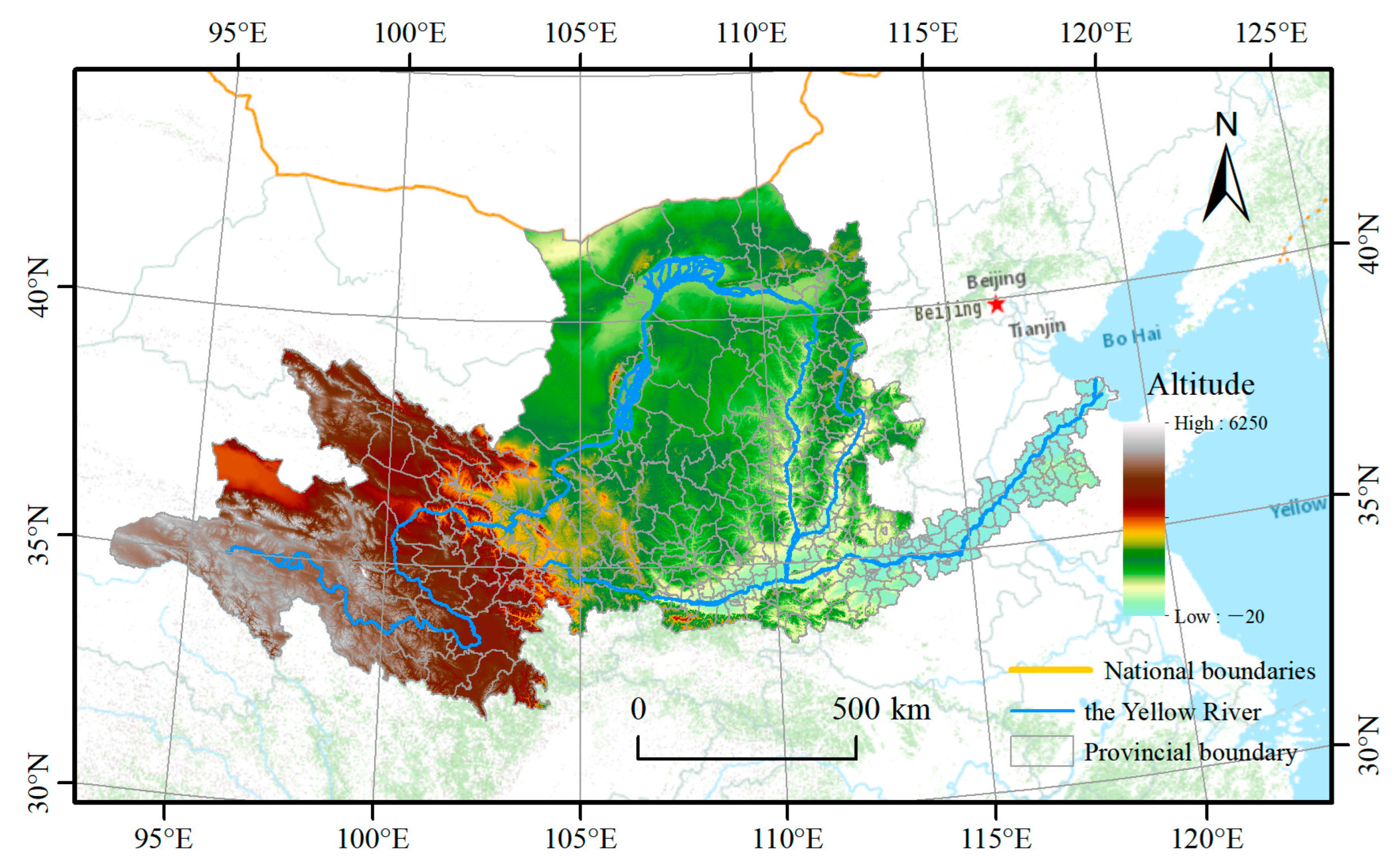
2.1. The Location of the Study Area

Occupying an area of 7.95 × 10⁵ km² with jurisdiction of 423 counties (cities, districts, banners), the Yellow River Basin (31°15′~42°83′ N, 91°71′~120°17′ E) consists of complex and diverse terrains with an altitude of −20~6250 m experiencing mountains, plateaus, and plains from west to east in China (Figure 1). The climatic conditions in the region have evolved from the arid climate in the northwest to the monsoon climate in the east. The average annual temperature is 10.2 °C [35]. Grassland, woodland, and arable land are widely distributed in the basin [36]. By the end of 2020, the Yellow River Basin had a total population of 420 million, and a regional annual GDP of 2.39 billion yuan. The basin is abundant in water, energy, coal mines, and other resources. It forms a vital component of China’s “two screens and three belts” ecological security strategic framework, playing an essential role in the integrated advancement of the regional economy and ecological equilibrium. The eastern part of the Yellow River Basin is mainly urban landscape and farmland landscape. With the westward movement, the landscape types are gradually transformed into grassland landscapes, desert landscapes, and mountain landscapes. The study of Ess and ESTSs in the Yellow River Basin under different landscape types provides reference for the improvement of the regional ecological environment and sustainable development.

2.2. Data

This study employed a multi-source dataset comprising remote sensing images, meteorological data, soil data, topographic data, and socio-economic data collected between 2000 and 2020 (

Table 1. Data sources.

Data Type	Data Name	Data Format	Data Source
Remote sensing images	Landsat-OLI and Landsat-TM images	30 m × 30 m	Geospatial Data Cloud (https://www.gscloud.cn/, accessed on 8 May 2021)
Meteorological data	monthly total solar radiation, monthly sunshine duration, monthly average temperature, and monthly total rainfall	meteorological stations	China Meteorological Data Center (http://data.cma.cn/, accessed on 11 May 2021)
Soil data	Sand, silt, clay, organic carbon, nitrogen, phosphorus, potassium	1 km × 1 km	Chinese soil dataset (V1.1) in the World Soil Database (HWSD)
Topographic data	DEM, slope	30 m × 30 m	Geospatial Data Cloud (https://www.gscloud.cn/, accessed on 8 May 2021)
Socio-economic data	Population and economic data	Statistics	“China County Economic Statistical Yearbook”, provincial and municipal statistical yearbooks, and socio-economic statistical bulletins (https://www.cnki.net/, accessed on 18 March 2022)

). Notably, the Landsat-OLI and Landsat-TM images were predominantly sourced from the Geo-spatial Data Cloud Platform (http://www.gscloud.cn/, accessed on 8 May 2021), featuring a spatial resolution of 30 m. Based on the classification system of the dynamic remote sensing survey database of national basic resources and environmental background, the land use types were classified into six categories, including cultivated land, forest land, grassland, water area, construction land, and unused land [37]. Meteorological data from meteorological stations, encompassing monthly total solar radiation, monthly sunshine duration, monthly average temperature, and monthly total rainfall, were acquired from the China Meteorological Data Center (http://data.cma.cn/, accessed on 11 May 2021).

Soil data, which encompassed sand, silt, clay, organic carbon, nitrogen, phosphorus, and potassium, were derived from the Chinese soil dataset (V1.1) in the World Soil Database (HWSD). Its spatial resolution was 1 km. Terrain data, such as slope and DEM data, were sourced from the Geospatial Data Cloud with a spatial resolution of 30 m. Socio-economic statistical data were primarily obtained from the China Statistical Yearbook at the county level, as well as more detailed provincial and municipal statistical yearbooks and the socio-economic statistical bulletin.

Finally, a spatial database for ES research was constructed using the ENVI and ArcGIS software platforms. The procedures are briefly described as follows: The above data were first processed as a 0.5 km × 0.5 km grid. Then, the map file data were processed by map digitization, geometric correction, mask clipping, file format conversion, vector data rasterization, etc. In addition, the non-digitized data were input into the attribute database. All of the processed map data and attribute data were finally stored in the spatial database of the ESs.

These datasets were obtained from official websites and books and thus have high quality to help obtain more accurate results. For instance, the remote sensing data in the Geospatial Data Cloud are from the National Public Science Data Center for Basic Disciplines of China, affiliated with the Ministry of Science and Technology of China. The meteorological data of the China Meteorological Data Center were produced by the China Meteorological Administration. Soil data are from the World Soil Database (HWSD) of the Food and Agriculture Organization of the United Nations. The China County Economic Statistical Yearbook, including socio-economic data, is an official book published annually by the National Bureau of Statistics of China.

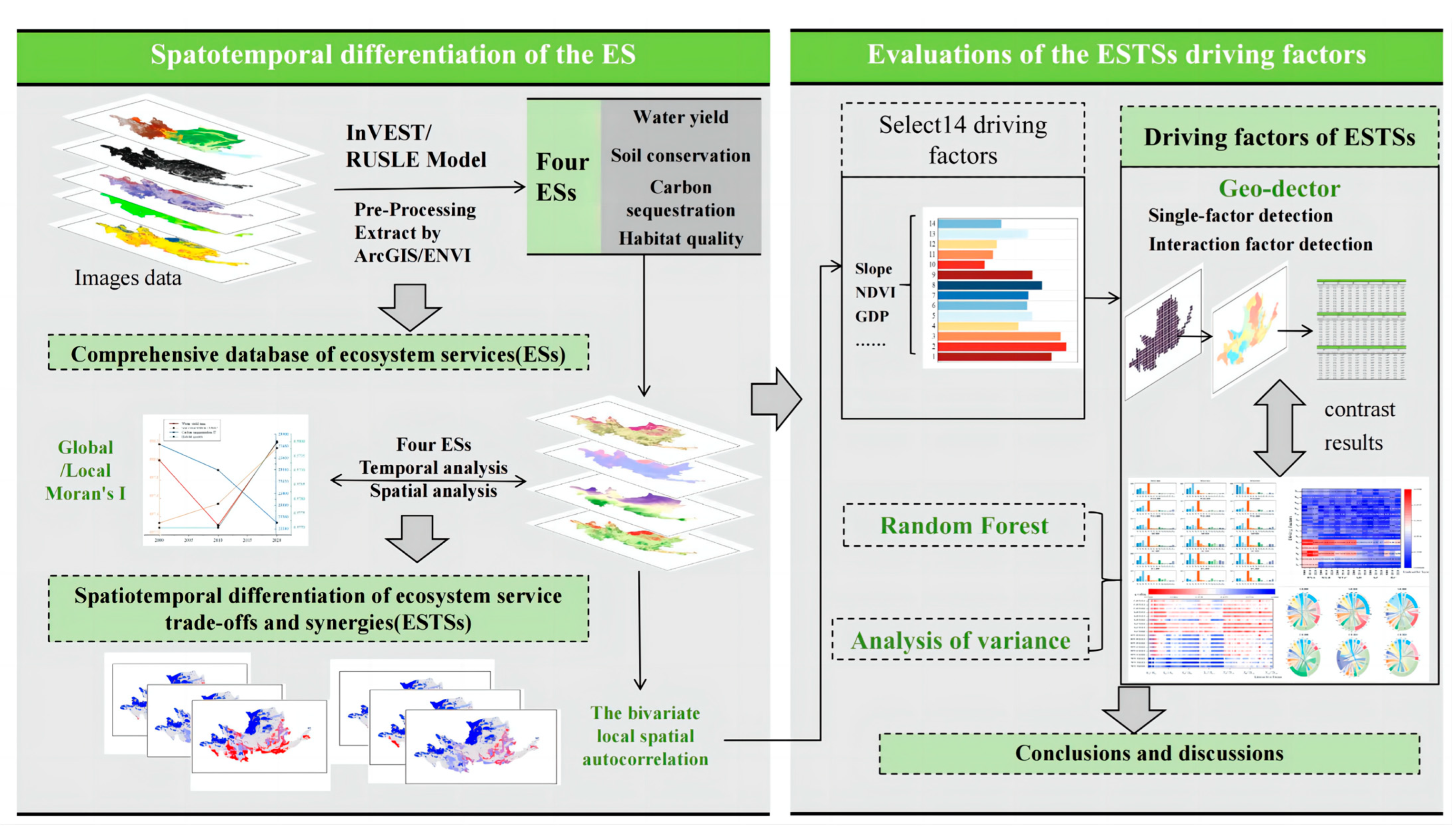
2.3. Research Framework

To comprehensively investigate the current state of ESs, elucidate the trade-offs and synergistic interactions, and unveil the driving factors behind their spatio-temporal differentiation, a quantitative evaluation framework has been designed (Figure 2). Firstly, based on the remote sensing imagery, meteorological, soil, and socio-economic statistical data, a spatial dataset for ES research in the Yellow River Basin was established. The InVEST model and RULSE model were employed to gauge four key ESs. Based on GeoDA, the bivariate spatial autocorrelation analysis method was then utilized to examine the relationship between ESTSs while affirming the global Moran’s I. Subsequently, the primary driving factors influencing the spatiotemporal distribution of ESTSs were explored through Geo-detector, encompassing the characterization of sample points, extraction of sample point attributes, and geographic detector assessment. Ultimately, the random forest and ANOVA were used to validate the reasonability of the driving forces behind the ESTSs. The findings will enable us to provide a scientific foundation for ecosystem management.

2.4. Methods

2.4.1. Measurement of ES Functions

(1)

Water yield

The InVEST model’s water yield operates by estimating the water supply for each grid within a watershed through a comprehensive analysis of climate, topography, soil, and vegetation characteristics. By subtracting the actual evapotranspiration per unit area, the module yields the actual water availability for the region [38].The InVEST model was utilized to calculate the water yield of the ESs, employing the following main formula [39]:

$$WR=min(1,\frac{249}{Velocity})\times min(1,\frac{0.9\times TI}{3})\times min(1,\frac{Ksat}{300})\times Yield$$

(1)

where WR represents the water conservation capacity, Velocity stands for flow velocity coefficient, TI denotes the topographic index, and K_sat indicates the saturated hydraulic conductivity of soil erosion.

(2)

Soil conservation

The RUSLE model offers the capability to calculate soil conservation within individual pixels. Its driving parameters primarily include the rainfall erosivity factor, soil erodibility factor, slope length and steepness factor, vegetation cover, and effectiveness of soil conservation measures [40]. The required data for the model encompass remote sensing imagery, meteorological data, digital elevation models (DEMs), as well as vegetation and soil type information. The RUSLE model was employed to estimate the soil conservation of the ESs, mainly relying on the following formula [41]:

$$Ac=R\times K\times L\times S\times (1-C-P)$$

(2)

where Ac and R represent the soil conservation capacity and precipitation erosion factor, respectively. S stands for slope factor. K denotes the soil erosion factor. C and P represent vegetation cover and water and soil conservation. L denotes the slope length factor.

(3)

Carbon sequestration

In terms of carbon storage, the InVEST model employs data regarding different land use types and corresponding carbon pool densities to assess carbon storage across various time periods and land categories [38]. The carbon sequestration was acquired by the InVEST model, which is estimated by the four basic carbon pools: aboveground biomass, underground biomass, soil, and dead organic matter [35,42]:

$$C_{totalx}=(C_{abovex}+C_{belowx}+C_{soilx}+C_{deadx})\times A_x$$

(3)

where C_totalx refers to the total carbon density (t/hm²) for the xth type of LULC, C_abovex is the biogenic carbon density above ground (t/hm²⁾ for the xth type of LULC, C_belowx represents the underground biocarbon density (t/hm²) for the xth type of LULC, C_soilx denotes the soil carbon density (t/hm²) for the xth type of LULC, C_deadx represents the dead organic matter (t/hm²) for the xth type of LULC, while A_x is the area (hm²) for the xth type of LULC.

(4)

Habitat quality

The habitat module of the InVEST model evaluates habitat quality based on land use information and the presence of stressors impacting biodiversity. By considering different land use types as representative of specific ecosystem types or human-induced disturbance factors, the model effectively captures and evaluates the spatial distribution of habitat quality, taking into account the suitability of each ecosystem type for supporting plant and animal life, as well as the intensity of threats posed by human disturbances [38]. The InVEST model can effectively combine regional land cover with biodiversity threat factors [43,44]:

$$Q_{pq}=H_q[1-\left(\frac{D_{np}^2}{D_{nq}^2+L^2}\right)]$$

(4)

where D_nq indicates the threat level of p in land-use type q, H_q indicates the ecological suitability of q, and L denotes the constant. The habitat quality [0–1] is categorized into five grades using the equal interval classification method. Higher grade values indicate a better $Q_{pq}$ [43,44].

2.4.2. Measurement of ESTSs

The GeoDA software was utilized to assess the degree of association and spatial distribution characteristics of ESs. The corresponding formula is below [45]:

$$I=\frac{n\sum _{i=1}^n\sum _{j=1}^n|X_j-\overline{X}||X_i-\overline{X}|}{\sum _{i=1}^n\sum _{j=1}^n{w}_{ij}{|X-\overline{X}|}^2}$$

(5)

where $I$ stands for Moran’s I and n indicates the total of spatial units. $X_i \mathrm{a}\mathrm{n}\mathrm{d} X_j$ represents the characteristic attribute value of the spatial units i and j. Moran’s I > 0 represents the synergistic between ESs, and the greater the value, the more powerful the synergy effect; Moran’s I < 0 represents the trade-off between ESs, and the smaller the value, the more powerful the trade-off effect; Moran’s I = 0 represents the randomness between ESs.

The bivariate local spatial autocorrelation is measured as follows [28]:

$$I_{lf}=Z_i^l\sum _{J=1}^n{w}_{ij}{Z}_j^f$$

(6)

where $I_{lf }$ is local bivariate Moran’s I, n denotes the total number of grid cells, $w_{ij}$ represents a spatial weight matrix that measures the correlation between grid cells of i and j, and $Z_i^l$ and $Z_j^f$ represent the normalized values. The local bivariate Moran’s I was visualized by generating a cluster plot. Finally, both high–high and low–low agglomerations indicate the synergy relationship, while both high–low and low–high agglomerations indicate the trade-off relationship.

2.4.3. Evaluations of the Driving Factors of ESTSs

(1)

Selection of driving factors

ESTSs are influenced by a combination of natural, socio-economic, and regional policy factors. Based on data availability, 14 indicators were selected to represent the ESTSs (

Table 2. Explanatory variables of ESTS.

Driving Factors		Impact Factors		Variable Interpretation
Natural factors	Topographic conditions	X1	Elevation at altitude	DEM data for each regional unit is obtained based on ArcGIS/m
		X2	Slope	The average slope of each geographical unit is extracted based on each DEM data/°
	Climatic conditions	X3	Average annual temperature	The average temperature of each geographical unit is obtained based on ArcGIS spatial interpolation/°C
		X4	Average annual precipitation	The average annual precipitation of each geographical unit is obtained based on ArcGIS spatial interpolation/mm
	Vegetation cover	X5	NDVI	The vegetation index of each geographical unit is obtained based on ArcGIS spatial interpolation
Socio-economic factors	Population size	X6	Population	Total population by region/person
		X7	Urbanization rate	Proportion of non-agricultural population in urban population by region/%
	Economic level	X8	GDP	GDP per region/yuan
		X9	Social fixed asset investment	The amount of social fixed asset investment in various regions/10,000 yuan
		X10	Grain production	Grain production per region/ton
		X11	The proportion of secondary and tertiary industries	Ratio output value of secondary and tertiary industries GDP in each region
		X12	Per capita disposable income of urban residents	Per capita disposable income of urban residents/yuan
		X13	Per capita disposable income of peasant residents	Per capita disposable income of peasant residents in each region/yuan
Regional policy factor	Ecological policy	X14	Ecological conversion Area	Conversion of cultivated land to other uses in each region/km2

). Among them, the natural environment covers the terrain conditions of altitude elevation and slope, the climatic conditions of temperature and precipitation, and the NDVI vegetation cover conditions. In terms of the social economy, the population size is represented by the total population and urbanization rate, and the economic level is characterized by the GDP, social fixed asset investment, grain yield, the proportion of industrial and service industries, urban per capita income, and rural per capita income. In terms of regional policy, the ecological conversion area is selected to represent the factors of ecological policy.

(2)

Evaluations of the driving factors

Geo-detector serves to identify spatial variations in geographic phenomena and uncover the underlying drivers behind them [46]. The method consists of four parts: risk detection, factor detection, ecological detection, and interaction detection. It possesses an edge over conventional statistical techniques, such as multiple linear regression and principal component analysis, by enabling the measurement of the unique effects of multiple factors and their interactions across various spatial scales [47].The main driving factors on ESTSs were first identified by the factor detection module in Geo-detector, and then the interaction effect between the driving factors was evaluated to screen the main two-way interactive effect by the interaction detection module of the Geo-detector.

The statistics of the contribution of a single driving factor are described below [48].

$$q=1-\frac{1}{N{\sigma }^2}{\sum }_{h=1}^L{N_h\sigma }_h^2$$

(7)

Here, the q [0–1] value denotes the contributions of the driving factors to ESTSs. The higher q corresponds to the greater influence of the independent variable X (driving factor X). σ² is the variance of the evaluation unit. N indicates the quantity of units. h, meanwhile, represents the quantity of clusters of driving factors, while N denotes the total of counties, and ${\sigma }_h^2$ denotes the variance of Ess for each spatial unit.

The Interaction detection module of the Geo-detector was employed to assess the interaction effects between driving factors, including nonlinear weakening, single-factor nonlinear weakening, two-factor enhancement, independent enhancement, and nonlinear enhancement.

The random forest and analysis of variance methods were adopted to verify the reasonableness of the driving factor results. Specifically, the relative importance of each driving factor to the ESTSs was measured by a random forest machine learning model. The interactive effect between two driving factors was measured by an analysis of variance model. The random forest model, a classification tree-based algorithm, enhances the predictive accuracy of the model by aggregating numerous classification trees [49]. This model represents a novel alternative to traditional machine learning methods like neural networks, particularly when handling extensive datasets. Random forests can be employed for both classification and regression tasks. In our study, the random forest model incorporated the 14 driver factors as input variables, while the classified ESETs served as the output variables. Selecting a sample size of 486, the factor score ranged from 0 to 100, wherein a higher score denoted greater significance of the factor. To assess the interrelation between two independent and dependent variables, the ANOVA method was implemented [50]. In this analysis, the 14 factors and their 91 interactions were used to evaluate the impact of these interaction values on ESTSs. The score ranged from 0 to 1, where a higher factor score indicated a greater degree of factor importance. The calculation principles and formulas of the specific model are shown in the thesis [51,52]. Finally, reasonable results for the evaluations of the driving factors were obtained by comparing the corresponding results from these methods.

3. Results

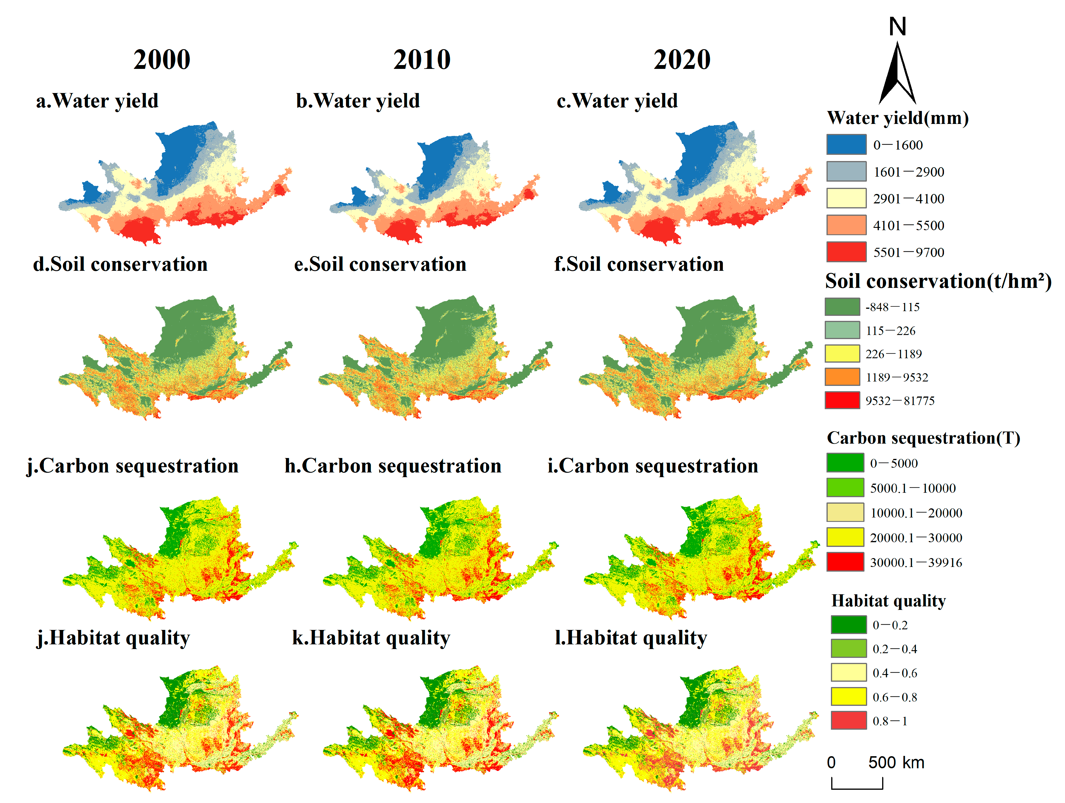
3.1. Spatio-Temporal Variations of ESs

The spatio-temporal variations of ESs during 2000–2020 are shown in Figure 3, and the statistics are listed in

Table 3. Average annual value of four ESs during 2000–2020.

Ess (Units)	2000	2010	2020	2000–2010		2010–2020
				Variation	Ratio/%	Variation	Ratio/%
Water yield (mm)	3348.56	3347.20	3348.93	−1.36	−0.04	1.73	0.05
Soil conservation (T/hm2)	897.33	897.54	898.15	0.21	0.02	0.61	0.07
Carbon sequestration (T)	23,483.32	23,439.60	23,350.51	−43.72	−0.19	−89.09	−0.38
Habitat quality	0.577	0.577	0.580	—	—	0.001	0.52

. It demonstrated that the ESs were distributed high in the east and low in the west. During this period, the overall spatial pattern for each ES changed faintly, while the local zone changed obviously.

Figure 3a–c show that the water yield represented a spatial pattern with highs in the south and lows in the northwest. The water yield volume decreased during 2000–2020 (see Table 3). Specifically, the regions with high water yield values were mainly focused on the southern part of the Weihe River Valley and the southeast of the Tibetan Plateau. The regions with low water yield values were mainly focused on the border area between the Loess Plateau and Alashan Plateau. In addition, water yield services formed a small-scale, low-value agglomeration area in the northwest of Qinghai.

Figure 3d–f show that soil conservation represented a gradual decrease from south to north, and the lowest values focused on the lower reaches of the Yellow River during 2000–2020. The soil conservation volume slightly increased from 2000 to 2020 (see Table 3). Specifically, the regions with high soil conservation values were mainly focused on the southern part of the Weihe River Valley, while the regions with low values were mainly focused on the junction of the Inner Mongolia Plateau, the Alashan Plateau and the Loess Plateau, and the lower reaches of the Yellow River. In addition, soil conservation formed a small-scale, low-value agglomeration area in the northwest of Qinghai.

Figure 3g–i show that carbon sequestration was distributed high in the southeast and low in the northwest in the Yellow River Basin during 2000–2020. The volume continued to decrease from 2000 to 2020 (see Table 3). Specifically, the regions with high carbon sequestration values were mainly focused on the southeast of the Tibetan Plateau and the southern part of the Fenwei River Valley. The regions with low carbon sequestration values were mainly focused on the junction of the Loess Plateau, the Inner Mongolia Plateau, and the Alashan Plateau. In addition, carbon sequestration formed small-scale, low-value agglomeration areas in northwestern Qinghai and northwestern Sichuan.

Figure 3j–l show that habitat quality is distributed high in the south and low in the northwest. The habitat quality volume first decreased and then increased from 2000 to 2020 (see Table 3). Specifically, the zones with high habitat quality focused on the southeast of the Tibetan Plateau, the Fenwei River Basin. The zones with low habitat quality were concentrated at the junction between the Loess Plateau and the Alashan Plateau. Additionally, it formed a small-scale, low-value agglomeration area in the northwest of Sichuan Province.

3.2. Spatio-Temporal Differences of ESTSs

3.2.1. Global Measure of ESTSs

The overall ESTSs were assessed using the global and local Moran’s I. Based on a 3 km × 3 km geographic grid unit, the global Moran’s I for ESs was calculated by ArcGIS and GeoDa, and

Table 4. Global Moran’s I indices between ESs.

ESs	2000			2010			2020
	Moran’s I	Z Value	p Value	Moran’s I	Z Value	p Value	Moran’s I	Z Value	p Value
Water yield—Soil conservation (WY-S)	0.440	427.527	0.001	0.440	427.611	0.001	0.440	427.351	0.001
Water yield—Carbon sequestration (WY-C)	0.483	447.377	0.001	0.462	433.133	0.001	0.455	427.545	0.001
Water yield—Habitat quality (WY-H)	0.512	472.213	0.001	0.487	453.272	0.001	0.477	445.666	0.001
Soil conservation—Carbon sequestration (S-C)	0.297	295.635	0.001	0.296	295.191	0.001	0.299	297.518	0.001
Soil conservation—Habitat quality (S-H)	0.294	288.686	0.001	0.289	282.575	0.001	0.290	282.389	0.001
Carbon sequestration—Habitat quality (C-H)	0.762	522.991	0.001	0.748	550.072	0.001	0.738	541.105	0.001

shows the results. The findings indicate that the global Moran’s I indices were positive and statistically significant (the absolute values of Z were all larger than 2.58, and the p values were lower than 0.01). It indicates that there were significant synergies between these ESs.

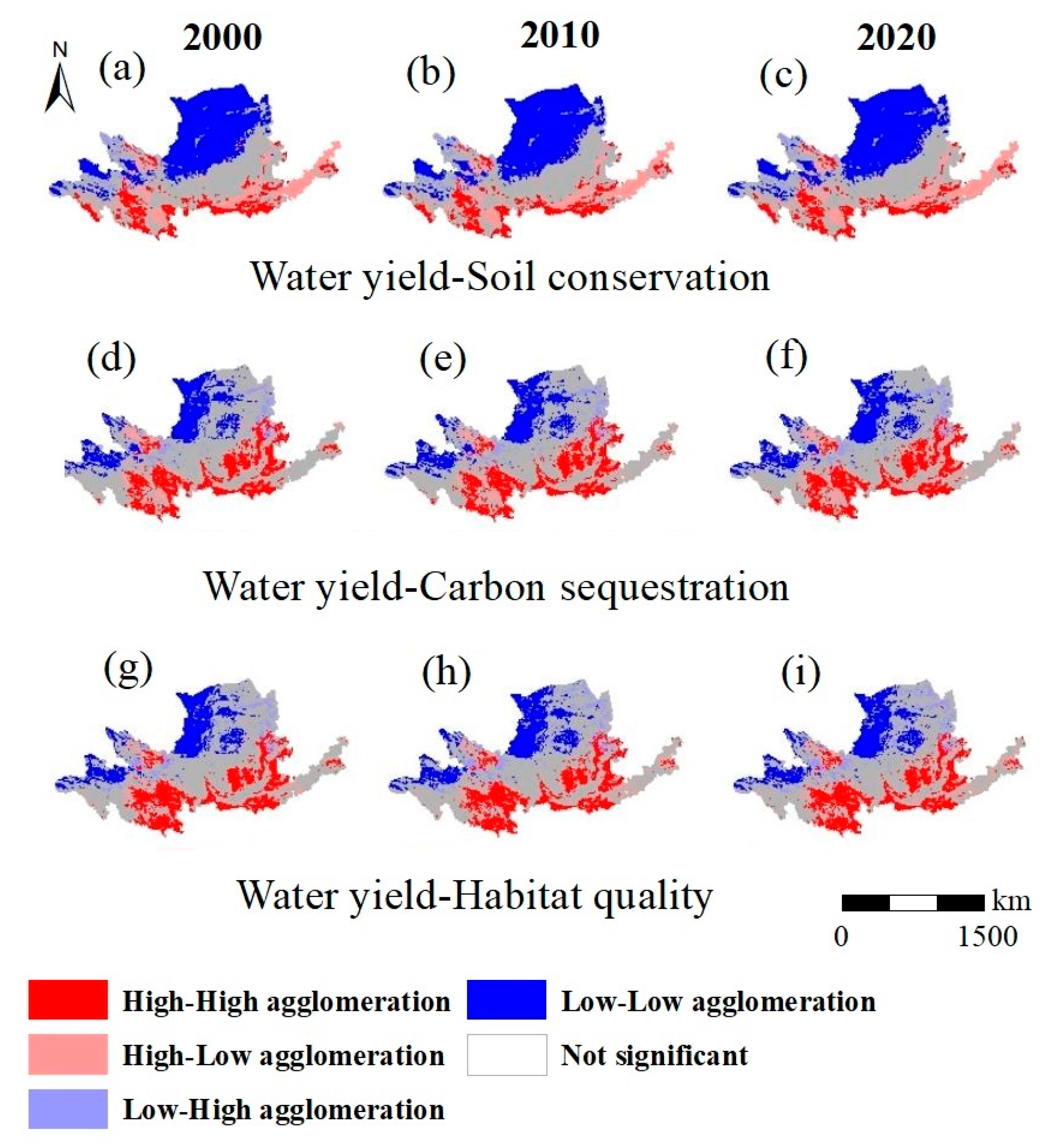
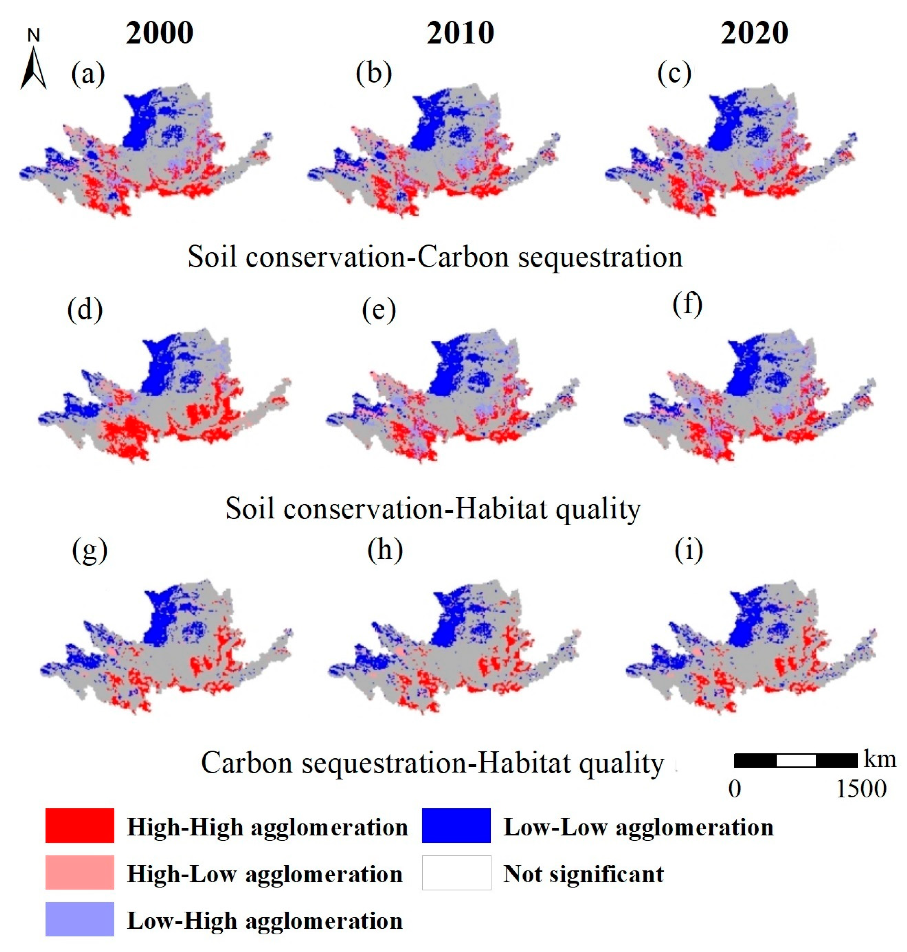
3.2.2. Spatio-Temporal Changes of ESTSs

Based on the local spatial autocorrelation analysis, the spatio-temporal variations of the ESTSs are shown in Figure 4 and Figure 5. Overall, more regions had significant spatial heterogeneity.

The spatial pattern changes in WY-S of ESTSs were mainly manifested as the expansion of the synergy zone and the contraction of the trade-off zone during 2000–2020 (Figure 4a–c and Figure 6a). The synergy zones between WY-S were mainly focused on the southeast of the Tibetan Plateau and the junction of the Inner Mongolia Plateau and the Loess Plateau, while trade-off zones were mainly focused on the northwest Huangshui Valley, Fenwei Valley, and the lower Yellow River Basin. Among them, the high–high synergy zones were focused on the southeast of the Tibetan Plateau and the southern part of the Weihe River Valley. Low–low synergy zones were focused on the junction of the Loess Plateau and the Inner Mongolia Plateau, and the Alashan Plateau. Whereas the high–low trade-off zone was focused on the North China Plain. The low–high trade-off zones were scattered in the Qinghai counties of Qilian, Tianjun, and Dulan.

The spatial pattern of WY-C of ESTSs was mainly manifested as the expansions of the synergy and trade-off zones during 2000–2020 (Figure 4d–f and Figure 6b). The synergistic relationship between WY-C was mainly focused on the Fenwei Valley, the southeast of the Tibetan Plateau, and the junction of the Inner Mongolia Plateau and the Loess Plateau. The trade-off zones were mainly along the Huangshui Valley and the Fenhe Valley. Among them, the high–high synergy zones were focused on the Fenwei Valley and the southeast of the Tibetan Plateau. The low–low synergy zone was mainly concentrated at the junction of the Loess Plateau and the Alashan Plateau. Whereas the high–low trade-off zones were focused on Qinghai Province and the low–high trade-off zones were sporadically distributed in Inner Mongolia province, Gansu province, and Helan and Ningxia.

The spatial pattern changes in WY-H of ESTSs were mainly manifested as the expansions of synergy and trade-off zones during 2000–2020 (Figure 4g–i and Figure 6c). The synergy zones between WY-H were mainly focused on the southeast of the Tibetan Plateau, the Fenwei Valley, and the junction of the Inner Mongolia Plateau and the Loess Plateau. The trade-off zones were mainly focused on the Huangshui Valley, the Fenhe Valley Basin, and the lower reaches of the Yellow River Basin. Among them, the high–high synergy zones were concentrated in the Fenwei Valley. The low–low synergy zones were focused on the junctions of the Loess Plateau, the Inner Mongolia Plateau, and the Alashan Plateau. Whereas the high–low trade-off zones were focused on the southeast of the Tibetan Plateau, there are also a few isolated areas of high–low trade-off zones in Henan province. The low–high trade-off zones concentrated on the eastern part of the Inner Mongolia Plateau, Huangshui Valley in Qinghai. In addition, there was sporadic distribution in the plains of the lower Yellow River.

The spatial pattern changes in S-C of ESTSs were mainly manifested as the expansion of the synergy zone and the contraction of the trade-off zone during 2000–2020 (Figure 5a–c and Figure 6d). The synergy relationships between S-C were mainly focused on the southeast of the Tibetan Plateau, the junction of the Inner Mongolia Plateau and the Loess Plateau, and the Fenwei Valley. The trade-off zones were mainly focused on the Huangshui Valley and the Fenhe Valley in the northwest. Among them, the high–high synergy zones were focused on the southeast of the Tibetan Plateau and the Fenwei Valley. The low–low synergy zones were mainly concentrated at the junction of the Loess Plateau and the Alashan Plateau. Whereas the high–low trade-off zones were concentrated in the Huangshui Valley. The low–high trade-off zones were scattered in the Fenhe Valley as well as its surrounding counties.

The spatial pattern changes in S-H of ESTSs were mainly manifested as the contraction of the synergy zone and the expansion of the trade-off zone during 2000–2020 (Figure 5d–f and Figure 6e). The synergy relationships between S-H were mainly focused on the southeast of the Tibetan Plateau, the junction of the Inner Mongolia Plateau and the Loess Plateau, and the Fenwei Valley. The trade-off zones were mainly focused on the Huangshui Valley and the Fenhe Valley. Among them, the high–high synergy zones were focused on the southeast of the Tibetan Plateau and Fenwei Valley. The low–low synergy zones were concentrated in the junction of Loess Plateau and Alashan Plateau. A sporadic low–low synergy zone was formed in the North China Plain. Whereas the high–low trade-off zones were concentrated in the southwest of the Huangshui Valley, and the low–high trade-off zones were scattered in the southeast of the Qinghai-Tibet Plateau, the Fenhe River Valley.

The spatial pattern changes in H-C of ESTSs were mainly manifested as the expansion of synergy and trade-off zones during 2000–2020 (Figure 5g–i and Figure 6f). The synergy relationships between H-C were mainly distributed at the junction of the Inner Mongolia Plateau and the Loess Plateau, and the trade-off zones were mainly distributed in Huangshui Valley. Among them, the high–high synergy zones were focused on the southeast of the Tibetan Plateau, and the Fenwei Valley and its surrounding areas. The low–low synergy zones were mainly concentrated at the junction of the Loess Plateau and Alashan Plateau. Whereas the high–low trade-off zones were focused on Huangshui Valley, the low–high trade-off zones manifested sporadic distributions on the border between Qinghai and Sichuan provinces.

In general, the ESTSs were patterned and showed a certain spatial stability. The ESTSs are mostly manifested as the expansion of the synergy zone and trade-off zone, followed by the contraction of the synergy zone and trade-off zone, and a few of them showed the contraction of the synergy zone and the expansion of the trade-off zone. The synergy zones tended to be concentrated in the northwest and southeast of the study area, mainly distributed in the southeast of the Qinghai-Tibet Plateau, the Fen-Wei River Valley, and the junction of the Inner Mongolia Plateau and the Loess Plateau. While the trade-off zones were more scattered than the synergy zone, they were mainly focused on the east-central and southwestern parts of the study area, involving the Fen Wei River Valley and the lower Yellow River Basin.

The southeastern part of the Tibetan Plateau and the southern part of the Weihe River Basin are characterized by their elevated terrain, favorable climate, and abundant precipitation, thus creating a conducive environment for water resource formation and ensuring a high water yield within the region. Moreover, the intricate river network in these areas, along with their rich soil cover and flourishing vegetation, further contributes to soil conservation. Vegetation cover plays a vital role in reducing soil erosion and facilitating water regeneration. Furthermore, dense vegetation fosters biodiversity, enabling the accumulation of carbon sequestration and promoting habitat quality, thereby upholding ecological balance.

In contrast, the juncture of the Loess Plateau and the Inner Mongolia Plateau, as well as the Alashan Plateau, exhibit a different scenario. These regions are characterized by low-lying terrain, arid climates, limited precipitation, poor soil quality, sparse vegetation, and reduced water use efficiency. Consequently, such unfavorable conditions lead to diminished water yields, inadequate soil conservation, and an overall unfavorable regional ecological environment. Thus, biodiversity growth is hindered, resulting in limited carbon sequestration and a compromised ecological balance, all of which contribute to the emergence of low–low synergistic zones.

Situated between the high–high synergy zones and the low–low synergy zones, the Fenwei River Valley and the lower reaches of the Yellow River exhibit a relatively balanced performance in terms of water resources, soil conservation, carbon storage, and habitat quality. The interactions between natural conditions and human activities in these areas not only facilitate resource utilization and development but also maintain ecological balance and environmental stability. Therefore, the distribution of ESTSs is primarily influenced by natural factors such as topography, climate, soil, and vegetation, coupled with the interplay of human activities.

In total, these factors determine the health status and resource utilization potential of ecosystems across various regions. In future endeavors concerning ecological protection and resource management, it is imperative to adopt region-specific policies and measures, taking into account the distinctive characteristics of each area. It helps promote the rational utilization of resources and foster sustainable development within the ecological environment.

3.3. Driving Factors of the Spatio-Temporal Differences of ESTSs

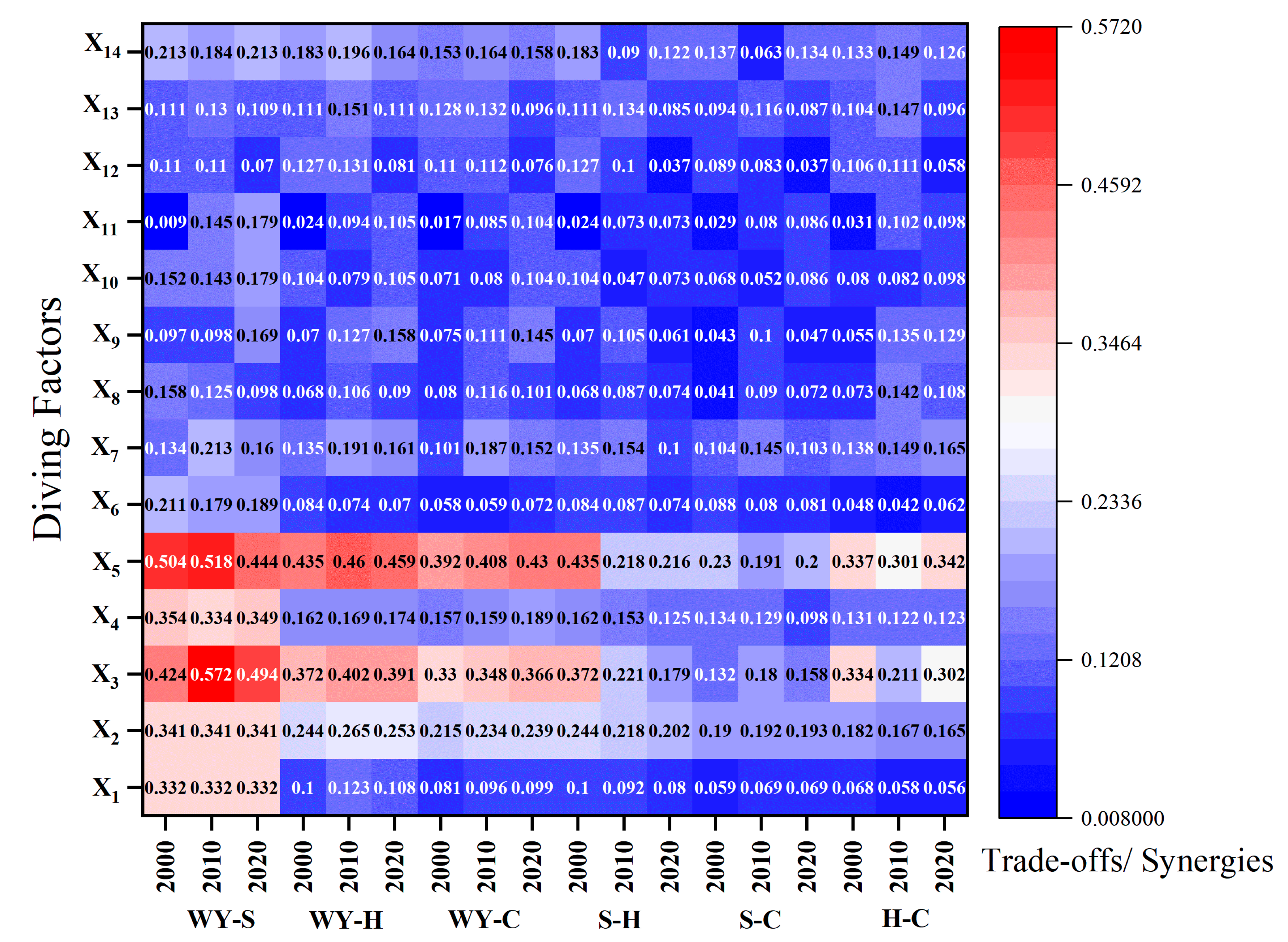
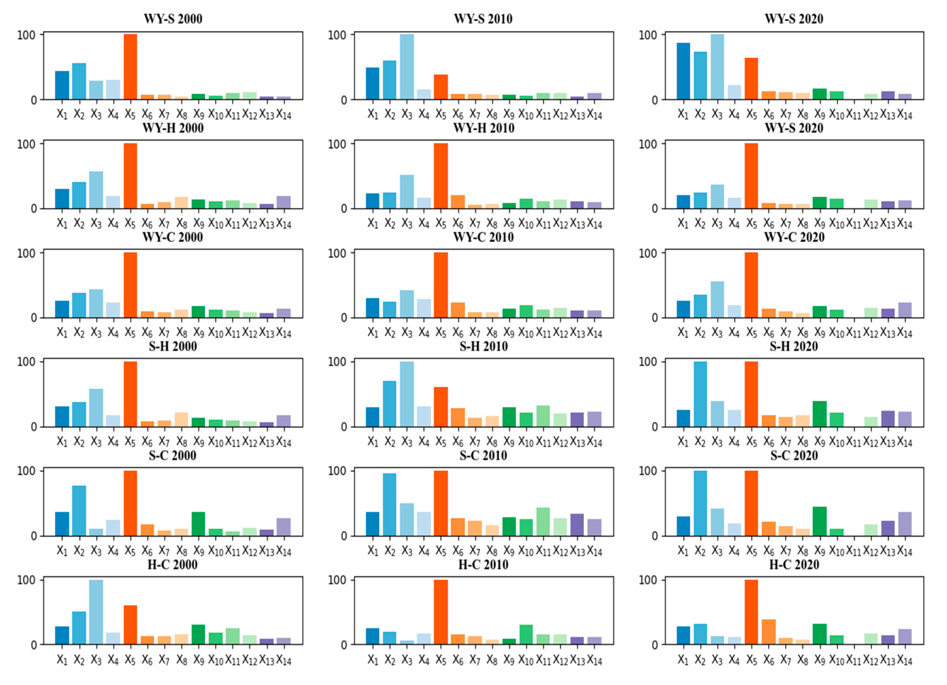
3.3.1. Driving Factor Detection

The factor detection in Geo-detector was used to assess the influence of determining factors on ES trade-offs (low–high trade-off zone and high–low trade-off zone, characterized by −1 in Geo-detector) and synergies (high–high synergy zone and low–low synergy zone, characterized by 1 in Geo-detector) as the dependent variables. The 14 indicators used as independent variables are shown in Table 2.

The contributions of the driving factors to ESTSs during 2000–2020 are posted in Figure 7, and the average explanatory power for each factor was obtained by averaging its contribution ratios in all six ESTSs across three years. Finally, the factors were ranked in terms of their explanatory abilities, as follows: X₅ (0.362) > X₄ (0.322) > X₂ (0.235) > X₃ (0.179) > X₁₄ (0.154) > X₇ (0.146) > X₁ (0.125) > X₁₃ (0.114) > X₉ (0.100) > X₁₀ (0.095) > X₈ (0.094) > X₁₂ (0.093) > X₆ (0.091) > X₁₁ (0.075).

Overall, natural driving factors (i.e., X₁–X₆) were the most significant for the ESTSs, and the highest contributions occurred in the WY-S of ESTSs. The influence of natural factors on WY-S is particularly obvious, as derived from Figure 6. Among the natural driving factors, NDVI (X₅) had the strongest impact on ESTSs. The NDVI also had the greatest impact on the enhancement of ESTSs, indicating that WY-S, WY-H, WY-C, S-H, S-C, and H-C continue to increase as with the increase in the NDVI. Following NDVI, the other natural factors (the average annual precipitation X₄, slope X₂, and temperature X₃) were also important. The impacts of ecological conversion area (X₁₄), urbanization rate (X₇), and elevation (X₁) were relatively smaller, reaching about 0.13, while the impacts of the rest of the factors, including rural per capita income (X₁₃), social investment in fixed assets grain production (X₉), grain production (X₁₀), GDP (X₈), urban per capita income (X₁₂), population (X₆), and the proportion of industrial and service industries (X₁₁), were the lowest, accounting for about 0.10. In addition, the explanatory power of the natural driving factors (X₁–X₅) on the ESTSs remained stable during 2000–2020, and the explanatory power of the socio-economic factors (X₆–X₁₃) and the regional policy factors (X₁₄) on the ESTSs showed an upward and downward trend, respectively.

In the random forest model, the 14 driver factors were used as the input variables, and the classified ESETs were used as the output variables. The sample size of the model was 486. The results of the random forest analysis for the two ESTSs in each year are shown in Figure 8. The score ranged from 0 to 100, with a higher factor score indicating the greater importance of the factor. The three-year average score for each driving factor ranged from 10.51 to 90.09, suggesting that the selected driving factors possess a degree of explanatory capability for the ESTSs. The factors were ranked in terms of their explanatory abilities as follows: X₅ (90.09) > X₂ (53.11) > X₃ (51.72) > X₁ (33.37) > X₄ (21.46) > X₉ (21.02) > X₁₄ (16.71) > X₆ (16.41) > X₁₀ (14.69) > X₁₂ (13.57) > X₁₃ (12.79) > X₈ (11.09) > X₁₁ (10.89) > X₇ (10.51).

It can also be observed that the natural factors played the most crucial role in the spatio-temporal differentiation of ESTSs, especially the NDVI score reaching 90.09. The regional policy factor (i.e., ecological conversion area X₁₄) ranked second only to the natural factors. The socio-economic factors (i.e., X₆–X₁₃) were the least important factors for the ESTSs. In addition, among the six ESTSs in the random forest method, WY-S was most strongly affected by natural factors. The influence of natural factors (X₁–X₅) on ESTSs remained unchanged, while the influence of socio-economic factors (X₆–X₁₃) and regional policy factors (X₁₄) on ESTSs showed an upward trend. Obviously, the findings obtained from the random forest method align closely with the factor detection in the Geo-detector method, demonstrating the driving factor detection results’ reasonability.

In general, natural factors are the most significant factors affecting the spatio-temporal differentiation of ESTSs, followed by the regional policy socio-economic factors. This has been well verified by the Geo-detector and random forests, which proves the rationality of the factor detection results. In addition, the influence of natural factors on ESTSs remained stable from 2000 to 2020, while the influence of socio-economic factors on ESTSs showed an upward trend, and the strongest influence of natural factors on ESTSs occurred in WY-S, which had also been demonstrated by the two methods.

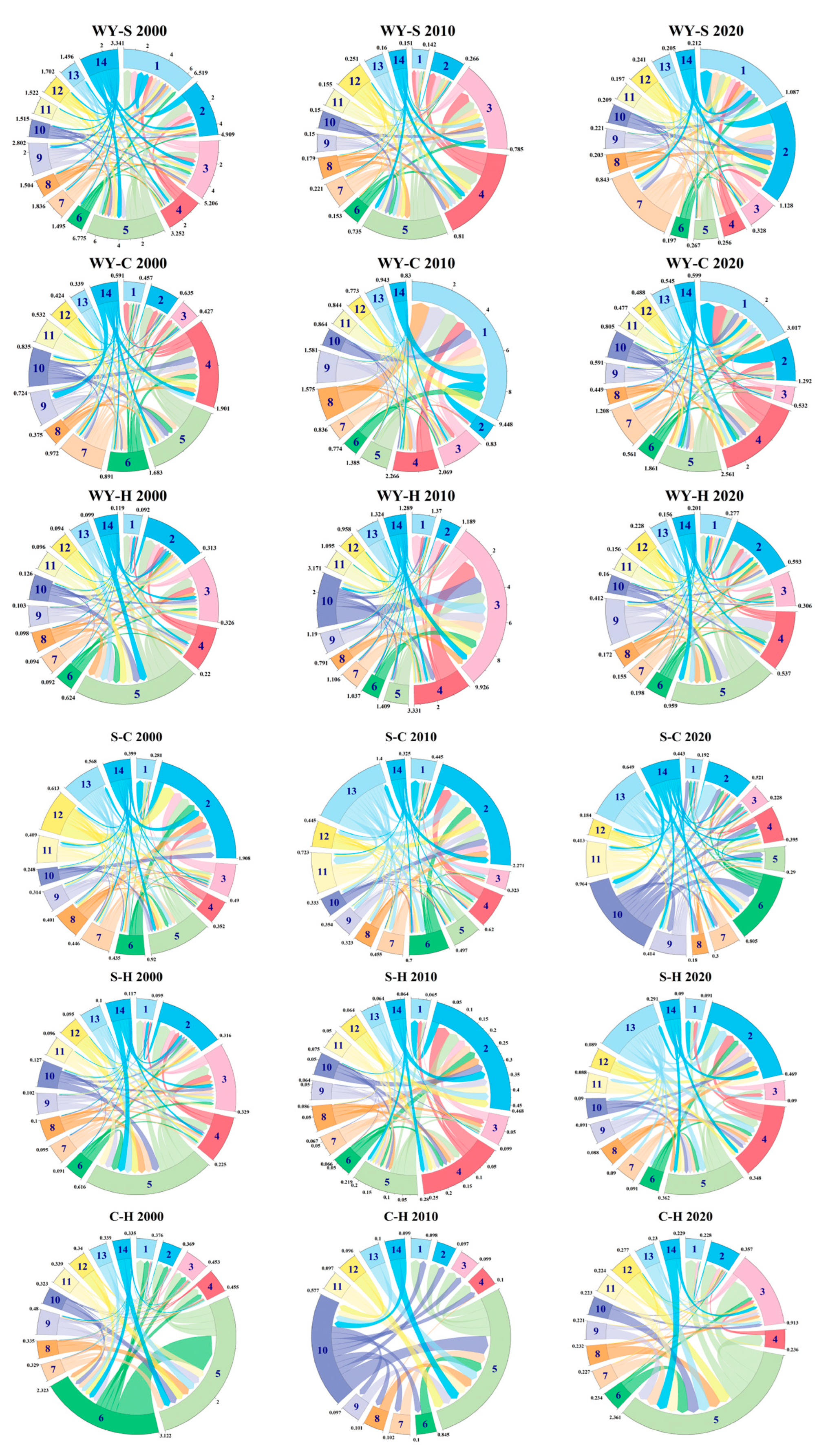
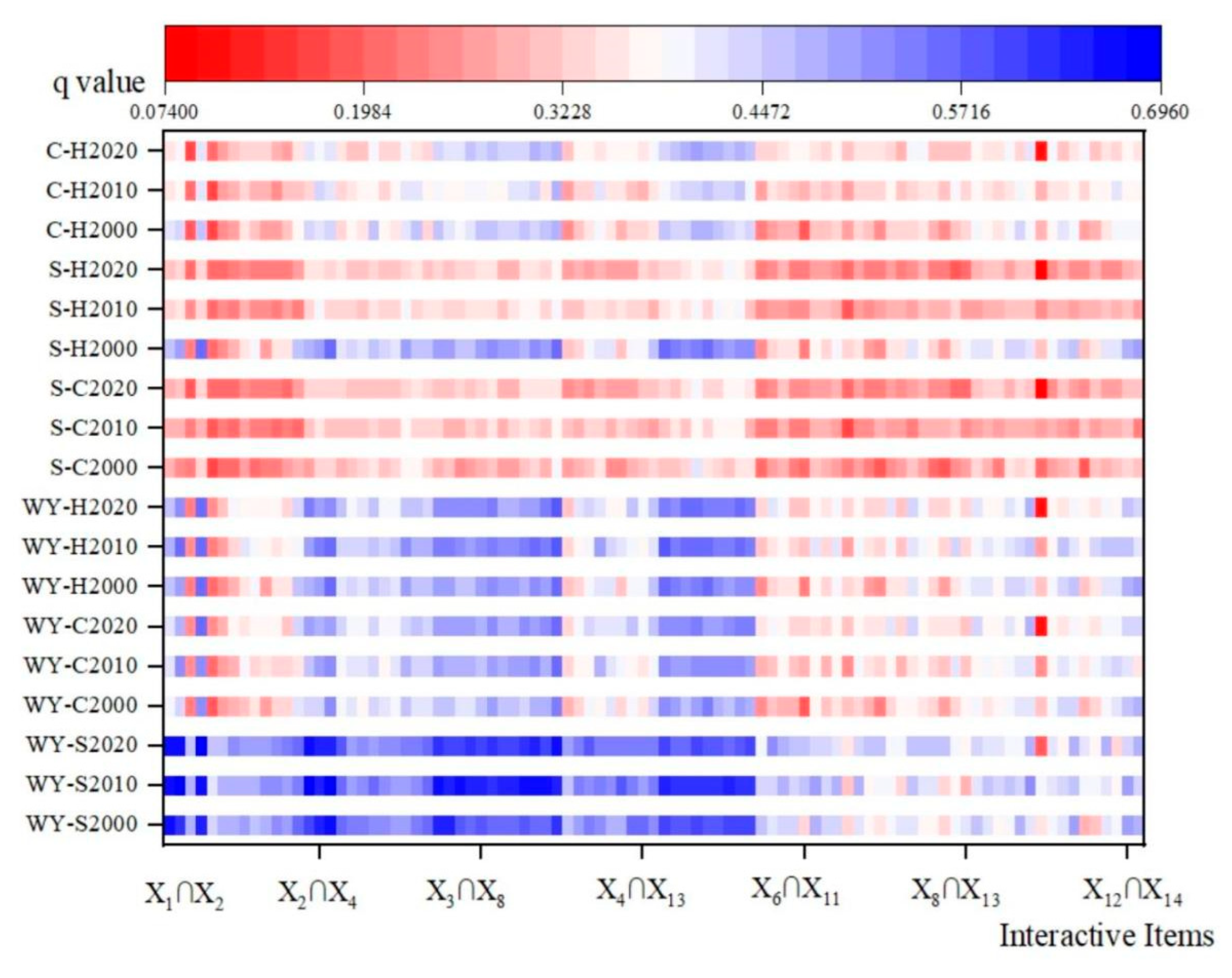
3.3.2. Interactive Effects of Driving Factors

The “Interactive detection” function of the Geo-detector was utilized to identify the pairwise interaction of the above 14 indicators. The 91 pairwise interaction results are shown in Figure 8, in which the abscissa represents the 91 two-way interaction combinations consisting of X₁–X₁₄, and the ordinate indicates the q value of the ESTSs. For more explicit expression, the top ten items with the highest q values among 91 pairwise interactions were selected for analysis (

Table 5. The top 10 interactive detection results of the spatial-temporal differentiation of ESTSs in Yellow River Basin.

WY-S						WY-C
2000		2010		2020		2000		2010		2020
Interactive	q value	Interactive	q value	Interactive	q value	Interactive	q value	Interactive	q value	Interactive	q value
X1∩X2	0.659 *	X1∩X3	0.696 *	X1∩X5	0.687 *	X2∩X5	0.571 *	X4∩X5	0.576 *	X4∩X5	0.585 *
X2∩X5	0.657 *	X2∩X3	0.685 *	X2∩X3	0.673 *	X5∩X10	0.571 **	X5∩X6	0.572 **	X1∩X5	0.560 **
X1∩X5	0.652 *	X2∩X5	0.681 *	X1∩X3	0.666 *	X4∩X5	0.566 **	X2∩X5	0.571 *	X5∩X9	0.557 *
X3∩X4	0.651 *	X1∩X5	0.675 *	X1∩X2	0.659 *	X1∩X5	0.563 **	X1∩X3	0.564 **	X5∩X13	0.556 **
X2∩X4	0.642 *	X3∩X13	0.673 *	X4∩X5	0.658 *	X5∩X6	0.551 **	X1∩X5	0.562 **	X5∩X7	0.554 *
X3∩X5	0.634 *	X3∩X4	0.672 *	X2∩X4	0.654 *	X5∩X8	0.549 **	X3∩X13	0.562 **	X3∩X7	0.548 **
X4∩X5	0.619 *	X3∩X12	0.670 *	X3∩X13	0.651 **	X5∩X7	0.532 **	X5∩X7	0.559 *	X5∩X6	0.542 **
X1∩X3	0.617 *	X3∩X14	0.668 *	X2∩X5	0.638 *	X5∩X11	0.526 **	X5∩X13	0.558 *	X5∩X14	0.539 *
X5∩X6	0.603 *	X1∩X2	0.659 *	X3∩X8	0.633 **	X5∩X13	0.520 *	X5∩X9	0.553 *	X2∩X3	0.536 *
X5∩X7	0.602 *	X3∩X6	0.655 *	X3∩X4	0.632 *	X5∩X14	0.519 *	X5∩X10	0.552 **	X5∩X12	0.533 **
WY-H						S-C
2000		2010		2020		2000		2010		2020
Interactive	q value	Interactive	q value	Interactive	q value	Interactive	q value	Interactive	q value	Interactive	q value
X4∩X5	0.541 *	X4∩X5	0.567 *	X4∩X5	0.571 *	X2∩X5	0.571 *	X5∩X13	0.394 **	X5∩X12	0.387 **
X5∩X10	0.537 **	X5∩X6	0.529 **	X1∩X5	0.551 *	X5∩X10	0.571 **	X4∩X5	0.394 **	X5∩X13	0.383 **
X2∩X5	0.519 *	X2∩X5	0.523 *	X5∩X7	0.535 *	X4∩X5	0.566 **	X5∩X11	0.392 **	X5∩X7	0.375 **
X1∩X5	0.514 **	X5∩X13	0.521 *	X5∩X14	0.535 *	X1∩X5	0.563 **	X2∩X4	0.387 **	X4∩X5	0.367 **
X5∩X6	0.512 **	X5∩X8	0.521 *	X5∩X13	0.531 *	X5∩X6	0.551 *	X5∩X7	0.385 **	X5∩X9	0.360 **
X5∩X8	0.509 **	X3∩X13	0.519 **	X5∩X9	0.526 *	X5∩X8	0.549 **	X2∩X12	0.385 **	X3∩X12	0.360 **
X5∩X7	0.501 *	X5∩X10	0.519 **	X3∩X7	0.523 *	X5∩X7	0.532 **	X5∩X9	0.377 **	X2∩X13	0.358 **
X3∩X7	0.493 **	X5∩X11	0.517 *	X3∩X14	0.519 *	X5∩X11	0.526 **	X3∩X13	0.374 **	X3∩X9	0.352 **
X5∩X13	0.492 **	X1∩X5	0.515 *	X5∩X6	0.515 **	X5∩X13	0.520 **	X5∩X12	0.372 **	X3∩X7	0.351 **
X5∩X11	0.486 **	X5∩X12	0.512 *	X5∩X12	0.514 *	X5∩X14	0.519 *	X3∩X12	0.371 **	X5∩X10	0.351 **
S-H						H-C
2000		2010		2020		2000		2010		2020
Interactive	q value	Interactive	q value	Interactive	q value	Interactive	q value	Interactive	q value	Interactive	q value
X5∩X7	0.409 *	X5∩X11	0.384 **	X5∩X7	0.387 **	X4∩X5	0.487 **	X4∩X5	0.482 **	X5∩X7	0.491 *
X4∩X5	0.395 *	X2∩X12	0.382 **	X5∩X13	0.373 **	X5∩X7	0.479 **	X5∩X10	0.466 **	X3∩X13	0.484 **
X2∩X13	0.373 **	X5∩X7	0.373 **	X5∩X12	0.369 **	X5∩X10	0.475 **	X5∩X13	0.453 **	X5∩X13	0.481 **
X2∩X12	0.366 **	X5∩X13	0.372 **	X3∩X7	0.364 **	X1∩X5	0.464 **	X5∩X12	0.447 **	X5∩X10	0.478 **
X7∩X14	0.363 **	X5∩X12	0.365 **	X4∩X5	0.364 **	X3∩X7	0.458 *	X3∩X13	0.442 **	X5∩X11	0.478 **
X5∩X14	0.358 *	X4∩X5	0.365 **	X5∩X9	0.354 **	X2∩X7	0.456 **	X5∩X7	0.440 *	X4∩X5	0.477 **
X5∩X13	0.358 *	X2∩X4	0.364 **	X3∩X12	0.354 **	X3∩X12	0.454 **	X5∩X11	0.439 **	X5∩X9	0.468 *
X7∩X12	0.357 **	X3∩X7	0.362 *	X2∩X13	0.353 **	X3∩X14	0.452 *	X2∩X4	0.435 **	X3∩X14	0.458 **
X4∩X7	0.348 **	X5∩X8	0.354 **	X3∩X14	0.351 **	X3∩X4	0.452 *	X5∩X9	0.428 *	X5∩X8	0.456 **
X2∩X7	0.346 **	X3∩X12	0.349 **	X5∩X14	0.349 *	X5∩X11	0.452 **	X4∩X7	0.422 **	X5∩X12	0.455 **

Note: * represents two-factor enhancement and ** represents nonlinear enhance.

).

Table 5 shows the interaction between various factors had double factor enhancement and nonlinear enhancement effects on the spatio-temporal differentiation of ESTSs. Overall, the interaction driving forces of precipitation (X₄) and NDVI (X₅), NDVI (X₅) and urbanization rate (X₇), elevation of altitude (X₁) and NDVI (X₅), NDVI (X₅) and urban per capita income (X₁₂), and slope (X₂) and NDVI (X₅) had the highest degree of influence on the spatio-temporal differences of ESTSs, reaching about 0.47 of the q value on average. It is also easily concluded that the interactions between natural factors (i.e., elevation X₁, slope X₂, precipitation X₄, and NDVI X₅) were the most important for the ESTSs. Among them, the contribution of NDVI was the most significant. In addition, the urbanization rate (X₇) and the urban per capita income (X₁₂) from socio-economic factors contributed highly to the ESTSs. By comparing the variations in the q values of each interaction term over three years, it was determined that the driving capability of the interaction between different factors on ESTSs overall gradually weakened from 2000 to 2020.

The contributions of the interaction factors were evaluated by the analysis of variance method, posted in the chord diagram (Figure 9). The finding indicated that the natural factors (X₁–X₅) had overall large interactions with other factors. For instance, the width of X₄∩X₅ in WY-S 2010, X₂∩X₅ in WY-H 2000, X₂∩X₄ in S-H 2010, and X₅∩X₃ in C-H 2000 are the highest in Figure 10, indicating that these interaction values have the largest influence on ESTSs. By accumulating the contributions of two-way interactive factors for all the ESTSs from 2000 to 2020, the top 10 interactive driving factors were quantified. They were the elevation at altitude and NDVI (0.171), slope and NDVI (0.164), temperature and NDVI (0.163), temperature and precipitation (0.151), elevation at altitude and slope (0.146), elevation at altitude and temperature (0.140), precipitation and NDVI (0.132), elevation at altitude and precipitation (0.127), NDVI and population (0.117), and slope and temperature (0.112). Obviously, the interactions between natural factors contributed the most to the ESTSs. Among them, NDVI occupied the majority. It was also found that the influence of all the top 10 interactive driving factors on the interactions between ESTSs showed downward trends from 2000 to 2020.

In general, both the Geo-detector and the analysis of variance showed that the interactions between natural factors exerted the largest influence on ESTSs, followed by the interaction between natural factors and socio-economic factors. In particular, the interaction driving forces of elevation (X₁) and NDVI (X₅), slope (X₂) and NDVI (X₅), and average annual precipitation (X₄) and NDVI (X₅) had the highest influence degree for spatio-temporal differences of ESTSs, indicating the NDVI (X₅) was one of the most critical factors in participating in the construction of the main interactive factors affecting the ESTSs. In addition, the top-ranking interaction factors had diminishing explanatory power on the ESTSs during 2000–2020, which was identical to the interactive analysis of the Geo-detector methods.

Therefore, in the management of ESs in the Yellow River Basin, not only should we consider the function of natural factors (especially NDVI), but we should also pay attention to the coordination among natural, socio-economic, and regional policy driving factors through multiple regulation and supervision measures. Finally, an ES development model compatible with the level of social-economic development is built to avoid unreasonable or strong human interference with the ES system.

4. Discussion

The Yellow River Basin spans a large east-west and north-south range, making it a transitional zone between the east and west of China. The differences in topography and climate brought significant differences in the ES relationships. The spatio-temporal differentiations of ESs and ESTSs in the Yellow River Basin from 2000–2020 in this study were analyzed based on the dataset of natural, socio-economic, and regional policies. The result showed that there was a significant spatial difference in ES function, with a high distribution in the east and a low distribution in the west. The pattern results align with findings from prior research. (e.g., Fang et al., 2021; Yang et al., 2021) [36,53]. Overall, there were synergistic relationships between ESs. Some studies on the Loess Plateau regions, Yanan city, and Gansu province also prove this conclusion [18,54]. What’s more, the contributions of driving factors, including single factors and two-way interaction factors, were comprehensively evaluated for the spatio-temporal differentiation of the ESTSs. The findings indicated that natural factors and their interactions had the biggest influence on the spatio-temporal variation of ESTSs. The findings can offer backing for the ecological civilization construction and sustainable watershed management of the study area in the future.

For some foreign scholars, Gutsch et al. [55] demonstrated the trade-offs between ESs in German forests in balancing climate change, and the results showed that there are also trade-offs between water and habitat and water and carbon services. Taking the canton of Vaud as an example, Jaligot [56] analyzed the spatiotemporal patterns of 11 ESs from 1979 to 2014 and the historical evolution drivers of ecosystem services by using Spearman rank correlation, K-means clustering, and redundancy analysis. In addition, it is also found that different processes may result in changes in the same ecosystem services, depending on their spatial location. Jafarzadeh et al. [57] evaluated four ESs (carbon sequestration, water production, erosion control, and marketable products) and calculated synergies and trade-offs in the Mish-Khas Basin in western Iran. In addition, different scenarios were defined for each ES (water production, carbon sequestration, erosion prevention, and production income) by using different weights, with the best scenario to get the most benefit from the function being the best option.

Compared with these studies, more refined county-level scale datasets were used in this study. The more refined scales should help obtain more reasonable results for ESs and ESTSs. What’s more, comprehensive attribution analyses were used to identify the contributions of 14 driving factors associated with the natural, social-economic, and regional policy aspects of the ESTSs using the Geo-detector method. The geographic detector method can consider the influence of spatial and non-spatial factors on geographical phenomena at the same time and reveal spatial heterogeneity and spatial nonlinear relationships. In addition, the random forest and analysis of variance methods were used to validate the reasonability of major driving factors (single major factors and two-way major interactive factors) selected by the Geo-detector, respectively. Compared with Spearman rank correlation, K-means clustering, nonlinear programming methods, and other methods, Moran’s I can consider the spatial distribution and structure of data, and thus the analysis of spatial data is more accurate and comprehensive.

At the same time, it included policy-relevant factors (e.g., the area of ecological farmland returned to farmland is selected as the influencing factor). It is also found that foreign scholars also introduced marketable products and production income into the evaluation system, but four kinds of ESs were selected, which have more comprehensive consideration.

Water yield can reflect the ability of ecosystems to protect and utilize water resources. Soils are an important part of ecosystems to assess the resistance of ecosystems to soil erosion. Carbon is a key element in ecosystems, affecting climate change and ecosystem stability in watersheds. Habitat quality is the basis for biodiversity maintenance and ecosystem functioning. The four indicators are highly representative and comprehensive in assessing ESs. The selection of ESs contributes to a better understanding and conservation of biodiversity and helps decision-makers better understand the composition and function of ecosystems so as to develop more effective conservation and restoration measures. Furthermore, the categorization of various ESs enables more effective sustainable management of ecosystems, ensuring the judicious use and preservation of these services.

Additionally, this paves the way for the optimization of resource allocation and utilization, thereby facilitating the comprehensive utilization of the diverse ESs and enhancing resource utilization efficiency. For instance, Antonín Kusbach et al. [58] have suggested that merging new data sources with ecological classifications can yield high-quality information across multiple spatial, functional, and pertinent scales. This information can guide integrated land-use planning for forest management and assisted migration. Evaluating the different ecological classifications and delineating the advantages and disadvantages of various approaches can significantly contribute to the identification of enhanced management strategies in response to climate change and anthropogenic stress [59].

There were some inconsistent conclusions in some studies. For instance, Wang et al. posited that a trade-off existed between WY-S in the upper Han River Basin [60]. Chen et al. showed that there was a trade-off relationship between WY-C in the Tibetan Plateau [61], and Wang et al. put forward that S-C was a trade-off in the Shiyang River Basin [33]. There are two reasons for this: First, there will be differences in ES relationships in specific regions due to the different scales of geomorphology or administrative units. For instance, Wang et al. [33] adopted the sub-basin scale, while this study used the county scale. Secondly, the different research methods and the inconsistent evaluation periods also result in variations in outcomes. For instance, Chen et al. [61] adopted pixel-by-pixel correlation analysis for the Qinghai-Tibet Plateau during 1990–2015, while this study adopted spatial autocorrelation analysis for the whole Yellow River Basin during 2000–2020. What’s more, this study found that the amount of carbon sequestration showed a downward trend. The possible reason is as follows: Rapid expansion of the built-up lands due to accelerated urbanization caused encroachment on forests, grasslands, and farmlands, reducing overall carbon storage capacity in the study area over time. The study also had some limitations. For instance, the scale of the ESs can impact the performance of the ESTSs. Therefore, it is recommended that future studies analyze ESTSs at various spatial scales within the study area to further enhance the trustworthiness of evaluation findings. It was also noted that the accuracy of habitat quality has some uncertainties due to some subjective quantification of model parameters (e.g., the sensitivity of habitat types). Thus, the habitat quality estimation method should be improved and optimized in the future. Moreover, the contribution of the regional policy factor was difficult to accurately quantify. Because only one driving factor (i.e., ecological conversion area) in the regional policy aspect was selected for analysis, which may introduce certain uncertainty, it is necessary to further quantify regional policy factors to make the research results more robust.

Through the analysis of interactions and interdependencies among diverse ESs, this research enhances our comprehension of the intrinsic intricacy associated with ecosystem management and yields novel perspectives on sustainable resource allocation, thus offering new dimensions for sustainable resource management and environmental planning. Primarily, by quantifying the relationships between various services and exploring the synergistic effects among ecosystem services, potential win-win scenarios may be unveiled, which prove particularly invaluable for fostering coordinated growth between agricultural production and ecological conservation within the confines of the Yellow River Basin and analogous regions. Furthermore, by scrutinizing the spatial patterns of trade-offs and synergies, this study provides invaluable insights for landscape planning and ecosystem management strategies, endowing decision-makers with a deeper comprehension of the economic and ecological effects of adjusting diverse management choices.

As a critical area for agricultural production and ecological preservation in China, a comprehensive examination of the trade-offs and synergies inherent in the ESs within the Yellow River Basin can promote the coordinated development between agricultural production and ecological conservation. Additionally, it can serve as scientifically derived policy recommendations for government entities and decision-makers, facilitating the realization of “dual-carbon” objectives and sustainable development goals. Moreover, it can promote public consciousness with regards to ecological environmental protection and elevate the standard of ecological civilization construction.

As the world’s fifth-largest river, the Yellow River Basin presents profound significance in both the domestic and global spheres, characterized by an extensive agricultural heritage, abundant biodiversity, and a rich cultural legacy. The ecological status of the Yellow River Basin has a substantial impact not only on China’s ecological security and economic advancement but also on the global ecological environment and climate change dynamics. Consequently, the exploration of trade-offs and synergies within the ecosystem services of the Yellow River Basin can provide not only valuable references and experiences to ecological environmental protection in China but also scientific guidance for global ecological environmental preservation and sustainable development endeavors.

5. Conclusions

Clarifying the spatio-temporal patterns of the ESs and ESTSs and further detecting the contribution of their driving factors play a vital role in advancing regional ecological civilization construction and attaining sustainable watershed management by aligning economic development with ecological environmental protection. Using the Yellow River Basin as a study case, it not only demonstrated the spatio-temporal variation of ESs and ESTSs during 2000–2020, but also detected the contributions of driving factors measured by signal-factor main effects and binary-factor interaction effects. Here are the key conclusions:

(1)

In 2000–2020, the ESs of water yield, soil conservation, and habitat quality increased, while carbon sequestration decreased. There was significant spatio-temporal differentiation in ESs and ESTSs during 2000–2020, with a spatial pattern of high in the east and low in the west.

(2)

An overall synergistic relationship of ESs (water yield, soil conservation, carbon sequestration, and habitat quality) existed and showed a significant spatial heterogeneity distribution. The ESTSs were mostly manifested in three categories: the expansions of the synergy zone and trade-off zone occupying the majority, followed by the contraction of the synergy zone and trade-off zone, and a few of them with the contraction of the synergy area and the expansion of the trade-off zone. The synergy zones tended to be concentrated in the northwest and southeast of the study area, mainly distributed in the southeast of the Tibetan Plateau, the Fen-Wei River Valley, and the junction of the Loess Plateau and the Inner Mongolia Plateau. While the trade-off zones mainly focused on the east-central and southwestern parts of the study area, involving the Fen Wei River Valley and the lower Yellow River Basin.

(3)

Natural factors had the strongest explanatory power over the spatio-temporal differentiation of ESTSs, followed by regional policy factors and socio-economic factors. Among the driving factors, the NDVI of natural factors had the strongest influence on the ESTSs, and the strongest influence of natural factors on ESTSs occurred in WY-S. In addition, the influence of natural factors on ESTSs remained stable during 2000–2020, while the influence of socio-economic factors on ESTSs showed an upward trend. All of the above conclusions have been well verified by the Geo-detector and random forest methods.

(4)

Both the Geo-detector and the analysis of variance showed the interactions between natural factors had the strongest impact on ESTSs, followed by the interaction between natural factors and socio-economic factors. In particular, the interaction driving forces of elevation and NDVI, slope and NDVI, and average annual precipitation and NDVI had the highest influence degree for spatio-temporal differences of ESTSs. The NDVI (X₅) was one of the most critical factors in participating in the construction of the main interactive factors affecting the ESTSs in the Yellow River Basin. What’s more, the top-ranking interaction factors had diminishing explanatory power on the ESTSs during 2000–2020, which was proved by the two methods.

In light of these findings, the following suggestions for the ecological development of the Yellow River Basin are proposed:

Firstly, to mitigate carbon sequestration reduction, it is recommended to implement measures such as afforestation and vegetation restoration. These efforts can enhance vegetation coverage, increase forested areas, and thereby improve carbon sequestration capacity.

Secondly, it is crucial to coordinate regional resource allocation. Landscape planning and land use planning should prioritize the synergistic relationship between different ecosystem services. Rational resource allocation and cooperative protection of areas will optimize the provision of ecosystem services to enhance ecosystem synergies and reduce trade-offs.

Thirdly, given the significant impact of NDVI as a natural factor on ESs and ESTSs, it is recommended to strengthen vegetation cover monitoring and protection initiatives. Promoting vegetation growth is essential for enhancing the overall quality of ecosystem services. Attention should also be given to the interaction between natural factors, such as high altitude, NDVI, slope, and average annual precipitation, and their influence on ESTSs. Implementing corresponding ecological protection policies in the basin, which include vegetation preservation, prudent land resource utilization, and restoration, will improve water conservation, soil protection, carbon sequestration, and habitat quality.

Fourthly, it is essential to intensify research on the interaction between natural factors and socio-economic factors to delve deeper into their synergistic mechanisms. Collaborative efforts between downstream and upstream provinces should be enhanced, establishing a co-governance mechanism within the river basins to propel ecological protection and sustainable development. To address policy factors, it is recommended to provide robust policy guidance, formulate pertinent policies and measures, foster the development of the ecological economy, and promote public awareness of the ecological environment and its protection. This comprehensive approach will facilitate the coordinated development of ESTSs.

In conclusion, incorporating these considerations into the planning and management process will promote the sustainable development of ecosystem services in the Yellow River Basin.

References

1. Pan, J.H.; Dong, L.L. Spatial-temporal variation in vegetation net primary productivity and its relationship with climatic factors in the Shule River basin from 2001 to 2010. Hum. Ecol. Risk Assess. Int. J. 2018, 24, 797–818. (In Chinese) [Google Scholar] [CrossRef]
2. Zhang, Z.Y.; Liu, Y.F.; Wang, Y.H.; Liu, Y.L.; Zhang, Y.; Zhang, Y. What factors affect the synergy and tradeoff between ecosystem services, and how, from a geospatial perspective? J. Clean. Prod. 2020, 257, 120454. [Google Scholar] [CrossRef]
3. Huang, J.M.; Zheng, F.Y.; Dong, X.B.; Wang, X.C. Exploring the complex trade-offs and synergies among ecosystem services in the Tibet autonomous region. J. Clean. Prod. 2023, 384, 135483. [Google Scholar] [CrossRef]
4. Dou, H.S.; Li, X.B.; Li, S.K.; Dang, D.L.; Li, X.; Xin, L.Y.; Li, M.Y.; Liu, S.Y. Mapping ecosystem services bundles for analyzing spatial trade-offs in inner Mongolia, China. J. Clean. Prod. 2020, 256, 120444. [Google Scholar] [CrossRef]
5. Li, G.Y.; Jiang, C.H.; Gao, Y.; Du, J. Natural driving mechanism and trade-off and synergy analysis of the spatiotemporal dynamics of multiple typical ecosystem services in Northeast Qinghai-Tibet Plateau. J. Clean. Prod. 2022, 374, 134075. [Google Scholar] [CrossRef]
6. Chen, W.; Chi, G. Ecosystem services trade-offs and synergies in China, 2000–2015. Int. J. Environ. Sci. Technol. 2023, 20, 3221–3236. [Google Scholar] [CrossRef]
7. Li, Y.J.; Zhang, L.W.; Qiu, J.X.; Yan, J.P.; Wan, L.W.; Wang, P.T.; Hu, N.K.; Chen, W.; Fu, B.J. Spatially explicit quantification of the interactions among ecosystem services. Landsc. Ecol. 2017, 32, 1181–1199. (In Chinese) [Google Scholar] [CrossRef]
8. Zhong, L.N.; Wang, J.; Zhang, X.; Ying, L.X. Effects of agricultural land consolidation on ecosystem services: Trade-offs and synergies. J. Clean. Prod. 2020, 264, 121412. [Google Scholar] [CrossRef]
9. Shen, J.S.; Li, S.C.; Liu, L.C.; Liang, Z.; Wang, Y.Y.; Wang, H.; Wu, S.Y. Uncovering the relationships between ecosystem services and social-ecological drivers at different spatial scales in the Beijing-Tianjin-Hebei region. J. Clean. Prod. 2020, 290, 125193. [Google Scholar] [CrossRef]
10. Song, W.; Cao, S.S.; Du, M.Y.; Lu, L.L. Distinctive roles of land-use efficiency in sustainable development goals: An investigation of trade-offs and synergies in China. J. Clean. Prod. 2023, 382, 134889. [Google Scholar] [CrossRef]
11. Turner, K.G.; Odgaard, M.V.; Bøcher, P.K.; Dalgaard, T.; Svenning, J.C. Bundling ecosystem services in Denmark: Trade-offs and synergies in a cultural landscape. Landsc. Urban Plan. 2014, 125, 89–104. [Google Scholar] [CrossRef]
12. Zhang, H.; Deng, W.; Zhang, S.Y.; Peng, L.; Liu, Y. Impacts of urbanization on ecosystem services in the Chengdu-Chongqing Urban Agglomeration: Changes and trade-offs. Ecol. Indic. 2022, 139, 108920. [Google Scholar] [CrossRef]
13. Dong, W.; Wu, X.; Zhang, J.J.; Zhang, Y.L.; Dang, H.; Lv, Y.H.; Wang, C.; Guo, J. Spatiotemporal heterogeneity and driving factors of ecosystem service relationships and bundles in a typical agropastoral ecotone. Ecol. Indic. 2023, 156, 111074. [Google Scholar] [CrossRef]
14. He, D.; Zhou, J.; Gao, W.; Guo, H.C.; Yu, S.X.; Liu, Y. An Integrated CA-Markov Model for Dynamic Simulation of Land Use Change in Lake Dianchi Watershed. Acta Sci. Natural. Univ. Pekin. 2014, 50, 1095–1105. (In Chinese) [Google Scholar] [CrossRef]
15. Yuan, J.; Li, R.; Huang, K. Driving factors of the variation of ecosystem service and the trade-off and synergistic relationships in typical karst basin. Ecol. Indic. 2022, 142, 109253. [Google Scholar] [CrossRef]
16. Zhang, J.; Guo, W.; Cheng, C.J.; Tang, Z.Y.; Qi, L.H. Trade-offs and driving factors of multiple ecosystem services and bundles under spatiotemporal changes in the Danjiangkou Basin, China. Ecol. Indic. 2022, 144, 109550. [Google Scholar] [CrossRef]
17. Qian, C.Y.; Gong, J.; Zhang, J.X.; Liu, D.Q.; Ma, X.C. Change and tradeoffs-synergies analysis on watershed ecosystem services: A case study of Bailongjiang Watershed, Gansu. Acta Geophys. Sin. 2018, 73, 868–879. (In Chinese) [Google Scholar] [CrossRef]
18. Liu, Y.; Bi, J.; Lv, J.S. Trade-off and synergy relationships of ecosystem services and the driving forces: A case study of the Taihu Basin, Jiangsu Province. Acta Geophys. Sin. 2019, 39, 7067–7078. (In Chinese) [Google Scholar] [CrossRef]
19. Sun, Y.J.; Ren, Z.Y.; Hao, M.Y.; Duan, Y.F. Spatial and temporal changes in the synergy and trade-off between ecosystem services, and its influencing factors in Yanan, Loess Plateau. Acta Geophys. Sin. 2019, 39, 3443–3454. (In Chinese) [Google Scholar] [CrossRef]
20. Chen, S.; Li, G.; Zhuo, Y.; Xu, Z.; Ye, Y.; Thorn, J.P.R.; Marchant, R. Trade-offs and synergies of ecosystem services in the Yangtze River Delta, China: Response to urbanizing variation. Urban Ecosyst. 2022, 25, 313–328. (In Chinese) [Google Scholar] [CrossRef]
21. Chen, D.; Zeng, W.; Guo, K.R.; Wang, F.H. Study on Spatio-Temporal Evolution and Driving Forces of Ecosystem Services in the Three Gorges Reservoir Area from 2000 to 2020. J. Hum. Settl. West China 2023, 38, 127–134. [Google Scholar] [CrossRef]
22. Yin, L.C.; Wang, X.F.; Zhang, K.; Xiao, F.Y.; Cheng, C.W.; Zhang, X.R. Trade-offs and synergy between ecosystem services in National Barrier Zone. Geogr. Res. 2019, 38, 2162–2172. (In Chinese) [Google Scholar] [CrossRef]
23. Liu, Y.; Gao, Y.B.; Pan, Y.C.; Tang, L.N.; Lu, M.G. Spatial differentiation characteristics and trade-off/synergy relationships of rural multi-functions based on multi-source data. Geogr. Res. 2021, 40, 2036–2050. (In Chinese) [Google Scholar] [CrossRef]
24. Zeng, L. Research on the synergy relationship and spatial pattern optimization of ecosystem services in Guanzhong-Tianshui Economic Zone. Shaanxi Norm. Univ. 2019. (In Chinese) [Google Scholar] [CrossRef]
25. Tian, Y.C.; Wang, S.J.; Bai, X.Y.; Luo, G.J.; Xu, Y. Trade-offs among ecosystem services in a typical karst watershed, SW China. Sci. Total Environ. 2016, 566–567, 1297–1308. (In Chinese) [Google Scholar] [CrossRef] [PubMed]
26. Egoh, B.; Reyers, B.; Rouget, M.; Richardson, D.M.; Le Maitre, D.C.; Van Jaarsveld, A.S. Mapping ecosystem services for planning and management. Agric. Ecosyst. Environ. 2008, 127, 35–140. [Google Scholar] [CrossRef]
27. Li, D.H.; Zhang, X.Y.; Wang, Y.; Zhang, X.; Li, L. Evolution process of ecosystem services and the trade-off synergy in Xin’an River Basin. Acta Ecol. Sin. 2021, 41, 6981–6993. (In Chinese) [Google Scholar]
28. Nie, M.X.; Huang, S.H.; Pu, L.J.; Zhu, M.; Xiao, L. Spatial and Temporal Dynamics and Trade-offs and Synergies Analysis of Ecosystem Services in Rapidly Urbanizing Areas: A Case Study of the Su-Xi-Chang region. Res. Environ. Yangtze Riv. Ba. 2021, 30, 1088–1099. (In Chinese) [Google Scholar]
29. Ren, J.; Ma, R.R.; Huang, Y.H.; Wang, Q.X.; Guo, J.; Li, C.Y.; Zhou, W. Identifying the trade-offs and synergies of land use functions and their influencing factors of Lanzhou-xining urban agglomeration in the upper reaches of Yellow River Basin, China. Ecol. Indic. 2024, 158, 111279. [Google Scholar] [CrossRef]
30. Huang, L.; Zhu, P.; Cao, W. The impacts of the Grain for Green Project on the trade-off and synergy relationships among multiple ecosystem services in China. Acta Ecol. Sin. 2021, 41, 1178–1188. (In Chinese) [Google Scholar] [CrossRef]
31. Zhu, D.Z.; Chu, L.; Ma, S.; Wang, L.J.; Zhang, J.C. Tradeoff and Synergies Relationship Among Ecosystem Services. Res. Soil Water Con. 2021, 28, 308–315. (In Chinese) [Google Scholar] [CrossRef]
32. Mina, M.; Bugmann, H.; Cordonnier, T.; Irauschek, F.; Klopcic, M.; Pardos, M.; Cailleret, M. Future ecosystem services from European mountain forests under climate change. J. Appl. Ecol. 2017, 54, 389–401. [Google Scholar] [CrossRef]
33. Wang, B.; Zhao, J.; Hu, X.F. Analysison trade-offs and synergistic relationships among multiple ecosystem services in the Shiyang River Basin. Acta Ecol. Sin. 2018, 38, 7582–7595. (In Chinese) [Google Scholar]
34. Fang, L.L.; Xu, D.H.; Wang, L.C.; Niu, Z.G.; Zhang, M. The study of ecosystem services and the comparison of trade-off and synergy in Yangtze River Basin and Yellow River Basin. Geogr. Res. 2021, 40, 821–838. (In Chinese) [Google Scholar] [CrossRef]
35. Cao, Y.; Sun, Y.L.; Chen, Z.X.; Yan, H.; Qian, S. Dynamic changes of vegetation ecological quality in the Yellow River Basin and its response to extreme climate during 2000–2020. Acta Ecol. Sin. 2022, 11, 4524–4535. (In Chinese) [Google Scholar] [CrossRef]
36. Chen, Q.; Chen, Y.H.; Wang, M.J.; Jiang, W.G.; Hou, P. Change of vegetation net primary productivity in Yellow River watersheds from 2001 to 2010 and its climatic driving factors analysis. Chin. J. Appl. Ecol. 2014, 25, 2811–2818. (In Chinese) [Google Scholar] [CrossRef]
37. Liu, J.Y. Study on National Resources & Environment Survey and Dynamic Monitoring Using Remote Sensing. J. Remote Sens. 1997, 3, 225–230. (In Chinese) [Google Scholar] [CrossRef]
38. Sharp, R.; Tallis, H.T.; Ricketts, T. InVEST Version 3.2.0 User’s Guide; The Natural Capital Project: Stanford, CA, USA, 2015. [Google Scholar]
39. Zhang, L.; Dawes, W.R.; Walker, G.R. Response of mean annual evapotranspiration to vegetation changes at catchment scale. Water Resour. Res. 2001, 37, 701–708. (In Chinese) [Google Scholar] [CrossRef]
40. Renard, K.G.; Foster, G.R.; Weesies, G.A.; McCool, D.K.; Yoder, D.C. Predicting Soil Erosion by Water: A Guide to Conservation Planning with the Revised Universal Soil Loss Equation (RUSLE); US Department of Agriculture, Agricultural Research Service: Washington, DC, USA, 1997; Volume 703, p. 404. [Google Scholar]
41. Wischmeier, W.H.; Smith, D. Predicting Rainfall Erosion Losses: A Guide to Conservation Planning; Department of Agriculture, Science and Education Administration: Port Antonio, Portland, 1978. [Google Scholar]
42. Liu, Y.; Zhang, J.; Zhou, D.M.; Ma, J.; Dang, R. Temporal and Spatial variation of carbon storage in Shule River Basin based on InVEST model. Acta Ecol. Sin. 2021, 32, 1–14. (In Chinese) [Google Scholar]
43. Tang, F.; Fu, M.C.; Wang, L.; Zhang, P.T. Land-use change in Changli County, China: Predicting its spatial-temporal evolution in habitat quality. Ecol. Indic. 2020, 117, 106719. [Google Scholar] [CrossRef]
44. Zhou, X.Y.; He, Y.Y.; Huang, X.; Zhang, M.M. Topographic gradient effects of habitat quality and its response to land use change in Hubei Section of the Three Gorges Reservoir. Trans. Chin. Soc. Agric. Eng. 2021, 37, 59–267. (In Chinese) [Google Scholar] [CrossRef]
45. Zhu, Y.X.; Yao, S.B. The coordinated development of environment and economy based on the change of ecosystem service vale in Shanx Province. Acta Ecol. Sin. 2021, 41, 3331–3342. (In Chinese) [Google Scholar] [CrossRef]
46. Wang, Q.; Jiang, D.; Gao, Y.; Zhang, Z.; Chang, Q. Examining the Driving Factors of SOM Using a Multi-Scale GWR Model Augmented by Geo-Detector and GWPCA Analysis. Agronomy 2022, 12, 1697. [Google Scholar] [CrossRef]
47. Zhang, X.; Ruan, Y.; Xuan, W.; Bao, H.J.; Du, Z.H. Risk assessment and spatial regulation on urban ground collapse based on geo-detector: A case study of Hangzhou urban area. Nat. Hazards 2023, 118, 52–543. [Google Scholar] [CrossRef]
48. Wang, J.F.; Xu, C.D. Geodetector: Principle and prospective. Acta Geophys. Sin. 2017, 72, 116–134. (In Chinese) [Google Scholar] [CrossRef]
49. Mantas, C.J.; Castellano, J.G.; Moral-García, S.; Joaquín, A. A comparison of random forest based algorithms: Random credal random forest versus oblique random forest. Soft Comput. 2019, 23, 10739–10754. [Google Scholar] [CrossRef]
50. Emerson, R.W. MANOVA (Multivariate Analysis of Variance): An Expanded Form of the ANOVA (Analysis of Variance). J. Vis. Impair. Blind. 2018, 112, 125–126. [Google Scholar] [CrossRef]
51. Breiman, L. Random forests. Mach. Learn. 2001, 45, 5–32. [Google Scholar] [CrossRef]
52. Zhang, L. Principles and statistical applications of one-way and two-way ANOVA and testing. Math. Study Res. 2010, 7, 92–94. [Google Scholar]
53. Yang, J.; Xie, B.P.; Zhang, D.G. Spatial-temporal heterogeneity of ecosystem services trade-off synergy in the Yellow River Basin. Chin. Desert 2021, 41, 78–87. (In Chinese) [Google Scholar]
54. Xu, J.; Liu, H. Assessment and prediction of ecosystem services and their trade-offs and synergies in Gansu Province based on the GMMOP-PLUS model. China Environ. Sci. 2023, 11, 1–15. (In Chinese) [Google Scholar] [CrossRef]
55. Gutsch, M.; Lasch-Born, P.; Kollas, C.; Suckow, F.; Reyer, C.P. Balancing trade-offs between ecosystem services in Germany’s forests under climate change. Environ. Res. Lett. 2018, 13, 045012. [Google Scholar] [CrossRef]
56. Jaligot, R.; Chenal, J.; Bosch, M. Assessing spatial temporal patterns of ecosystem services in Switzerland. Landsc. Ecol. 2019, 34, 1379–1394. [Google Scholar] [CrossRef]
57. Jafarzadeh, A.A.; Mahdavi, A.; Shamsi, S.R. Assessing synergies and trade-offs between ecosystem services in forest landscape management. Land Use Policy 2021, 111, 105741. [Google Scholar] [CrossRef]
58. Kusbach, A.; Dujka, P.; Šebesta, J.; Lukeš, P.; DeRose, R.J.; Maděra, P. Ecological classification can help with assisted plant migration in forestry, nature conservation, and landscape planning. For. Ecol. Manag. 2023, 546, 121349. [Google Scholar] [CrossRef]
59. Ivanova, N.; Fomin, V.; Kusbach, A. Experience of Forest Ecological Classification in Assessment of Vegetation Dynamics. Sustainability 2022, 14, 3384. [Google Scholar] [CrossRef]
60. Wang, P.T.; Zhang, L.W.; Li, Y.J.; Jiao, L.; Wang, H.; Yan, J.P.; Lv, Y.H.; Fu, B.J. Spatial-temporal characteristics of ecosystem service trade-offs and synergies in the upper reaches of the Han River. Acta Geophys. Sin. 2017, 72, 2064–2078. (In Chinese) [Google Scholar] [CrossRef]
61. Chen, X.M.; Wang, X.F.; Feng, X.M.; Zhang, X.M.; Luo, G.X. Ecosystem service trade-off and synergy on Qinghai-Tibet Plateau. Geogr. Res. 2021, 40, 18–34. (In Chinese) [Google Scholar] [CrossRef]
Figure 1. The Location map of the Yellow River Basin.
Land 13 00369 g001
Figure 2. Research flowcharts.
Land 13 00369 g002
Figure 3. Spatio-temporal distribution of ESs during 2000–2020.
Land 13 00369 g003
Figure 4. The ESTSs between water yield and other ESs. (a) The ESTSs among WY-S in 2000; (b)The ESTSs among WY-S in 2010; (c) The ESTSs among WY-S in 2020; (d) The ESTSs among WY-C in 2000; (e) The ESTSs among WY-C in 2010; (f) The ESTSs among WY-C in 2020; (g)The ESTSs among WY-H in 2000; (h) The ESTSs among WY-H in 2010; and (i) The ESTSs among WY-H in 2020.
Land 13 00369 g004
Figure 5. The ESTSs among S-C, S-H, and H-C. (a) The ESTSs among S-C in 2000; (b) The ESTSs among S-C in 2010; (c) The ESTSs among S-C in 2020; (d) The ESTSs among S-H in 2000; (e) The ESTSs among S-H in 2010; (f) The ESTSs among S-H in 2020; (g) The ESTSs among C-H in 2000; (h) The ESTSs among C-H in 2010; and (i) The ESTSs among C-H in 2020.
Land 13 00369 g005
Figure 6. The percentages of ESTS areas and their changes from 2000 to 2020. (a) The percentage of Water yield- Soil conservation ESTS area in 2000–2020; (b) The percentage of Water yield - Carbon sequestration ESTS area in 2000–2020; (c) The percentage of Water yield- Habitat quality ESTS area in 2000–2020; (d) The percentage of Soil conservation - Carbon sequestration ESTS area in 2000–2020; (e) The percentage of Soil conservation - Habitat quality ESTS area in 2000–2020; and (f) The percentage of Habitat quality - Carbon sequestration ESTS area in 2000–2020.
Land 13 00369 g006
Figure 7. Driving factor detection results of ESTSs based on Geo-detector method in the Yellow River Basin. The colors ranging from blue to red in the figure indicate that the explanatory power will be increasing.
Land 13 00369 g007
Figure 8. Driving factor scores of the ESTSs based on the random forest method.
Land 13 00369 g008
Figure 9. The chord diagram of the interactions of driving factors with the ESTSs by the analysis of variance.
Land 13 00369 g009
Figure 10. The interactive detection results of ESTSs based on Geo-detector in the Yellow River Basin.
Land 13 00369 g010