Evaluating Machine Learning-Based Approaches in Land Subsidence Susceptibility Mapping

Abstract

Land subsidence (LS) due to natural and human-driven forces (e.g., earthquakes and overexploitation of groundwater) has detrimental and irreversible impacts on the environmental, economic, and social aspects of human life. Thus, LS hazard mapping, monitoring, and prediction are important for scientists and decision-makers. This study evaluated the performance of seven machine learning approaches (MLAs), comprising six classification approaches and one regression approach, namely (1) classification and regression trees (CARTs), (2) boosted regression tree (BRT), (3) Bayesian linear regression (BLR), (4) support vector machine (SVM), (5) random forest (RF), (6) logistic regression (LogR), and (7) multiple linear regression (MLR), in generating LS susceptibility maps and predicting LS in two case studies (Semnan Plain and Kashmar Plain in Iran) with varying intrinsic characteristics and available data points. Multiple input variables (slope, aspect, groundwater drawdown, distance from the river, distance from the fault, lithology, land use, topographic wetness index (TWI), and normalized difference vegetation index (NDVI)), were used as predictors. BRT outperformed the other classification approaches in both case studies, with accuracy rates of 75% and 74% for Semnan and Kashmar plains, respectively. The MLR approach yielded a Mean Square Error (MSE) of 0.25 for Semnan plain and 0.32 for Kashmar plain. According to the BRT approach, the variables playing the most significant role in LS in Semnan Plain were groundwater drawdown (20.31%), distance from the river (17.11%), land use (14.98%), NDVI (12.75%), and lithology (11.93%). Moreover, the three most important factors in LS in Kashmar Plain were groundwater drawdown (35.31%), distance from the river (23.1%), and land use (12.98%). The results suggest that the BRT method is not significantly affected by data set size, but increasing the number of training set data points in MLR results in a decreased error rate.

1. Introduction

Land subsidence (LS) is a global environmental issue caused by natural (e.g., earthquakes) or human-induced processes (e.g., over-exploitation of groundwater, dissolution of calcareous bedrock, extraction of natural gases and minerals) [1]. These processes can result in soil compaction and reduction in pore water pressure, leading to the gradual sinking of the ground surface and detrimental environmental and economic impacts [1,2]. Flooding and increased vulnerability to natural disasters are among the negative environmental consequences of LS [3,4], and the adverse impacts of LS on the economy include “lower agricultural productivity, water pollution, infrastructure destruction, and decreased real estate value” [5].

Some studies have examined LS using numerical and hydraulic modeling [6]. For example, Luo and Feng [7] simulated groundwater exploitation and its impact on LS using a finite element model for Cangzhou City, Hebei Province, China, and identified a one-month time lag between groundwater exploitation and LS. Shi et al. [8] studied the correlation between groundwater level and surface displacement by analyzing the impact of groundwater depression discs in different hydro-stratigraphic units using numerical simulation. To prevent further land subsidence, they concluded that excessive groundwater extraction must be prevented. In addition, several studies have used numerical groundwater models to investigate the relationship between groundwater extraction and aquifer deformation and to generate LS maps [9,10,11].

Numerous studies have demonstrated that machine learning approaches (MLAs) are more accurate than conventional parametric methods [12,13]. MLAs incorporate different historical datasets and analyze influential factors (e.g., soil characteristics, permeability) to classify and predict the LS susceptibility of a given area [2,3,4,5,6,7,8,9,10,11,12,13,14,15]. Using MLAs to detect LS-prone areas can enhance decision-making processes in water management and land use planning. Understanding the risk of subsidence enables planners to identify the most susceptible spots, allocate resources appropriately, and mitigate any further losses. In addition, these approaches can help identify potential areas of LS, allowing for improved use of targeted monitoring and early warning systems. Hence, several studies have been dedicated to investigating the accuracy and performance of different MLAs in modeling LS. Mohammady et al. [16] investigated land subsidence susceptibility in Semnan Plain, Iran, using Random Forest (RF). Rahmati et al. [17] compared the performance of the two models of maximum entropy (MaxEnt) and genetic algorithm rule-set production (GARP) for modeling land subsidence in Kashmar Plain (Iran). They concluded that the GARP model’s performance was better than MaxEnt. Arabaameri et al. [18] investigated the performance of four single and hybrid MLAs, including MaxEnt, general linear model (GLM), artificial neural network (ANN), and support vector machine (SVM), in Kashan plain (Iran). They highlighted the more accurate modeling abilities of the ANN model. Zhao et al. [19] combined a new approach to improve decision stump classification (DSC) with different MLAs (e.g., J48 decision tree, alternating decision tree) to map land subsidence susceptibility. They stated that their proposed approach enhanced the accuracy of LS prediction significantly. In another study, Mohammady et al. [16] investigated the accuracy of three MLAs, namely multivariate adaptive regression spline (MARS), mixture discriminant analysis (MDA), and boosted regression tree (BRT), for predicting LS susceptibility in Semnan Plain, Iran. They reported that MARS outperformed other MLAs in the study area. Liu et al. [20] addressed LS in urban planning and infrastructure management by using two machine learning models, including the extreme gradient boosting regressor (XGBR) and long short-term memory (LSTM). They identified groundwater level (GWL) and building concentration (BC) as key factors influencing LS. They also revealed that there could be a significant decrease in LS by 2040 in a scenario where the GWL (i.e., groundwater table) and BC impacts were reduced by 80%. This result highlights the importance of implementing strategic policy interventions. Eghrari et al. [21] conducted a study in Kashan Plain, Iran, to analyze the land subsidence susceptibility using RF and XGBoost MLAs and considered twelve influential factors, such as topography, vegetation, hydrological elements, and anthropogenic features.

MLAs can also be applied to understand how LS may be affected by climate change. By analyzing historical data and projecting future trends, MLAs can help identify areas where subsidence is expected to be most severe [22]. Collados-Lara et al. [23] developed a new method using regression models to investigate the impacts of climate change scenarios on land subsidence induced by groundwater drawdown. They reported a 54% increase in the LS rate in Vega de Granada in Spain under the representative concentration pathway (RCP) 8.5 climate change scenario.

Several studies indicate that MLAs have proven useful for estimating LS susceptibility as well as generating LS susceptibility maps, since MLAs do not rely on accurate data, which can be challenging to acquire. Nonetheless, a thorough evaluation of the performance of different MLAs has not been carried out, as most previous studies only compared a small number of approaches. Moreover, to obtain more accurate results, influential factors, including natural and human-induced factors, should first be determined and then employed in the modeling process. The aim of this study was thus to answer the following questions:

• Which MLA has higher accuracy for predicting LS in a given study area?
• Do different MLAs vary in performance in study areas with different inherent characteristics and status (e.g., groundwater drawdown)?

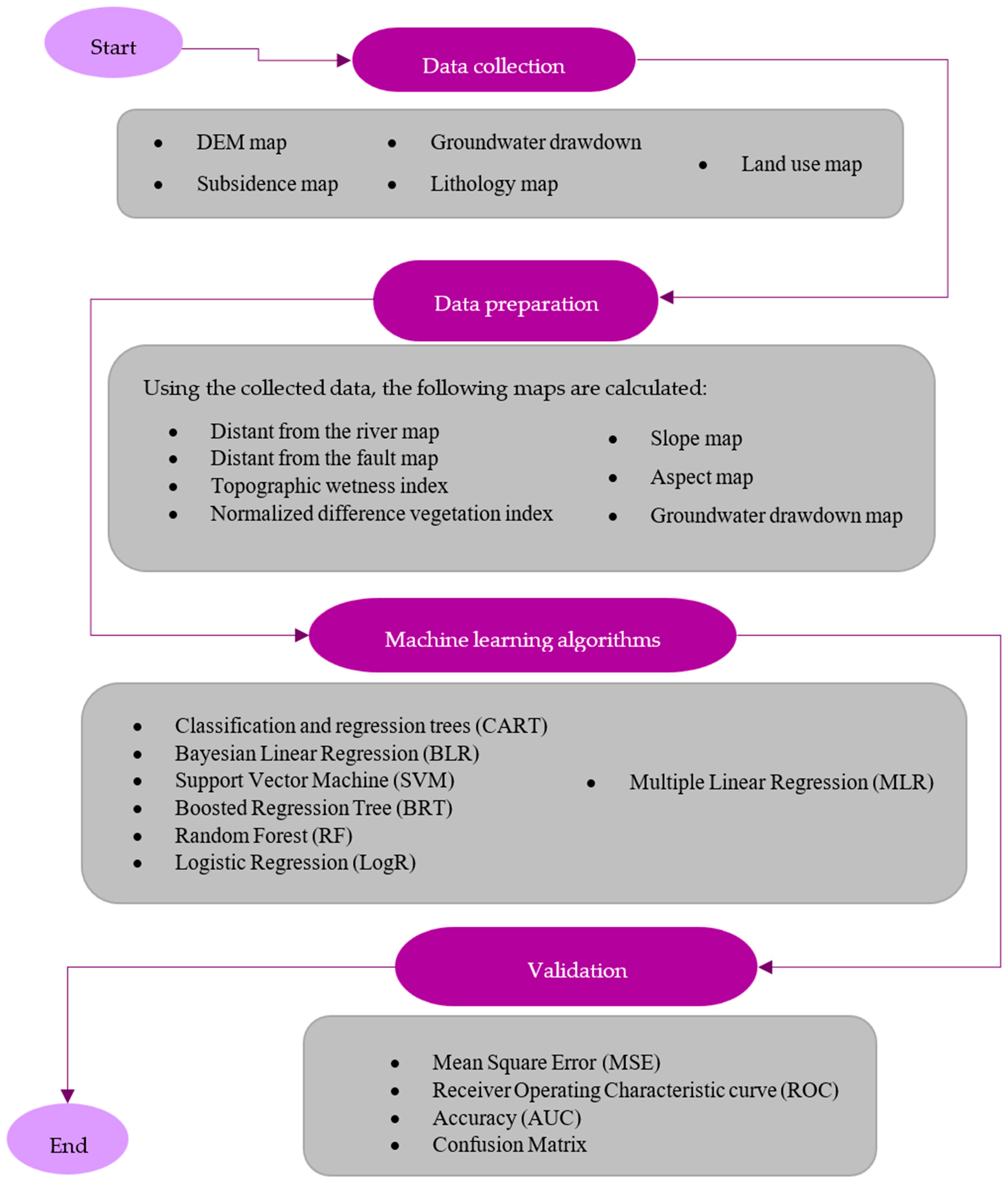
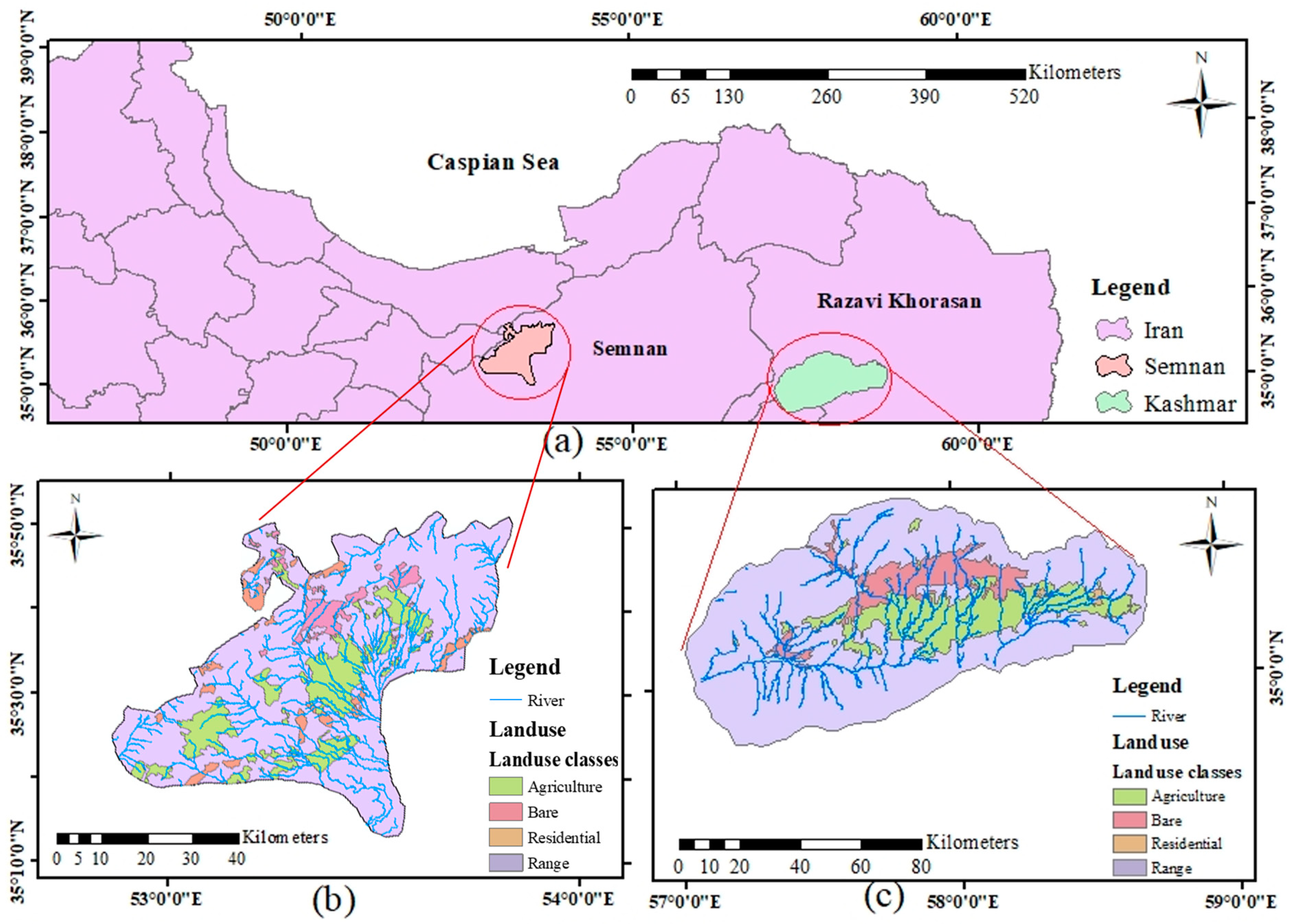
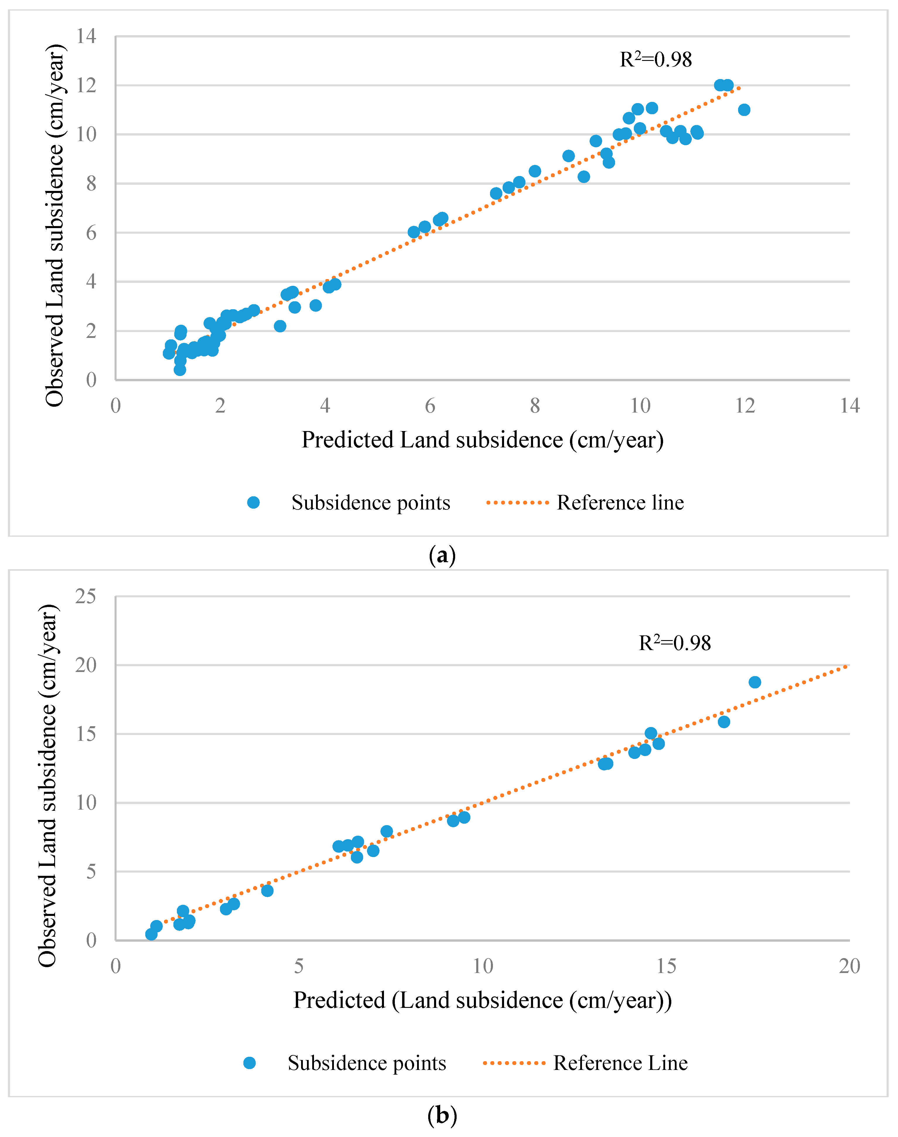
To achieve these aims, we scrutinized the performance of six classification MLAs (classification and regression tree (CART), Bayesian linear regression (BLR), SVM, boosted BRT, RF, and logistic regression (LogR)) and one regression method (multiple linear regression (MLR)) in identifying LS-prone areas and predicting the magnitude of LS. 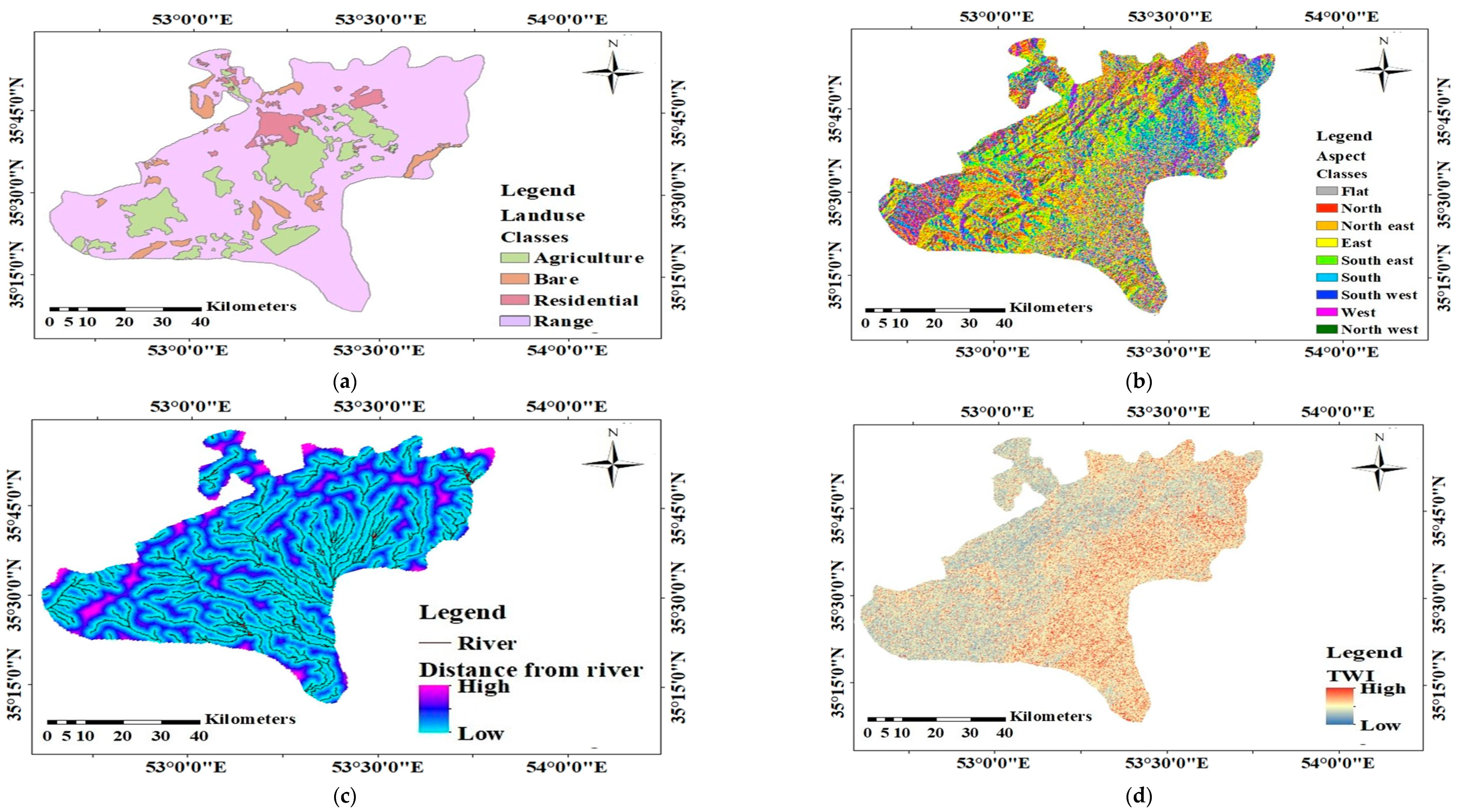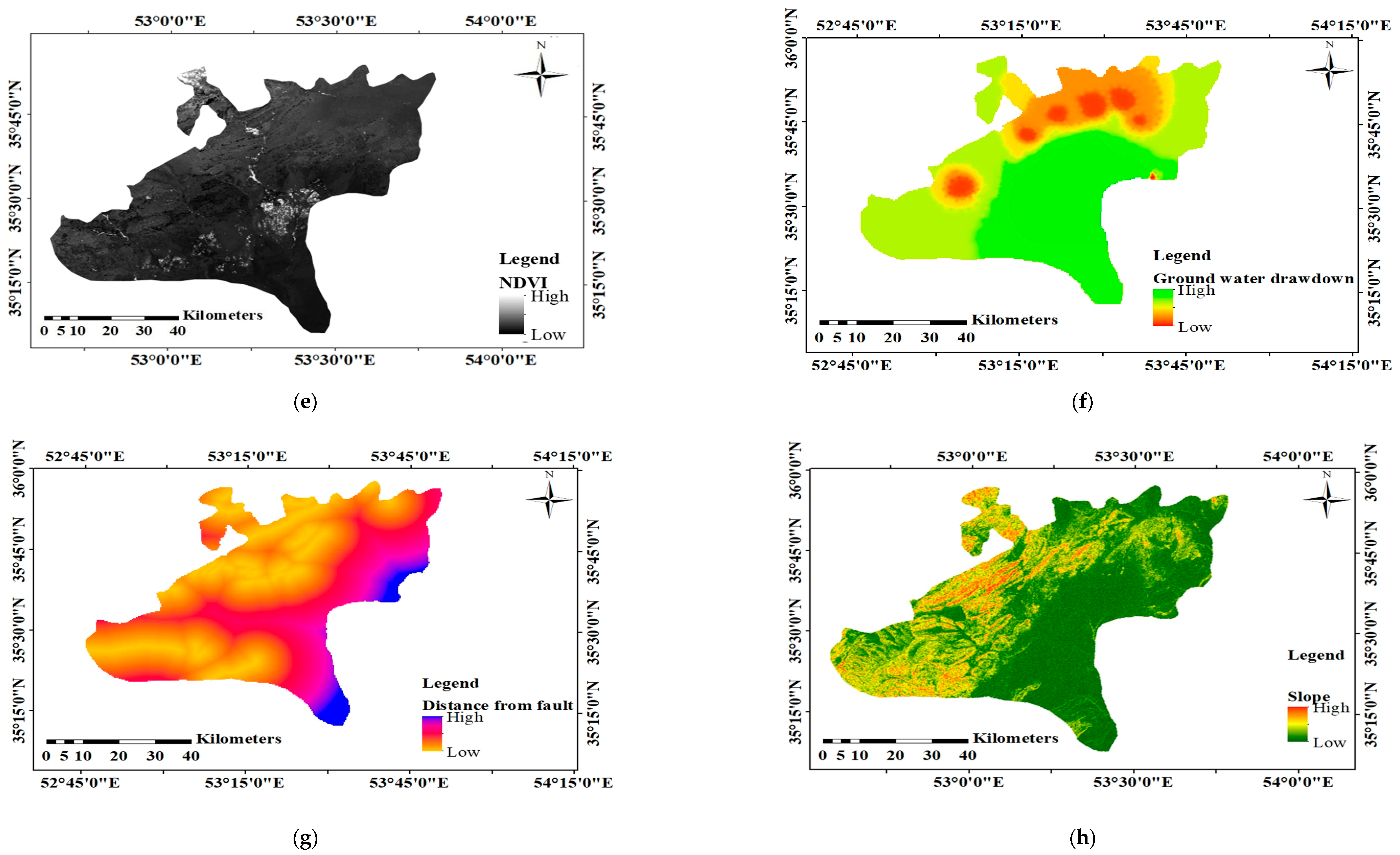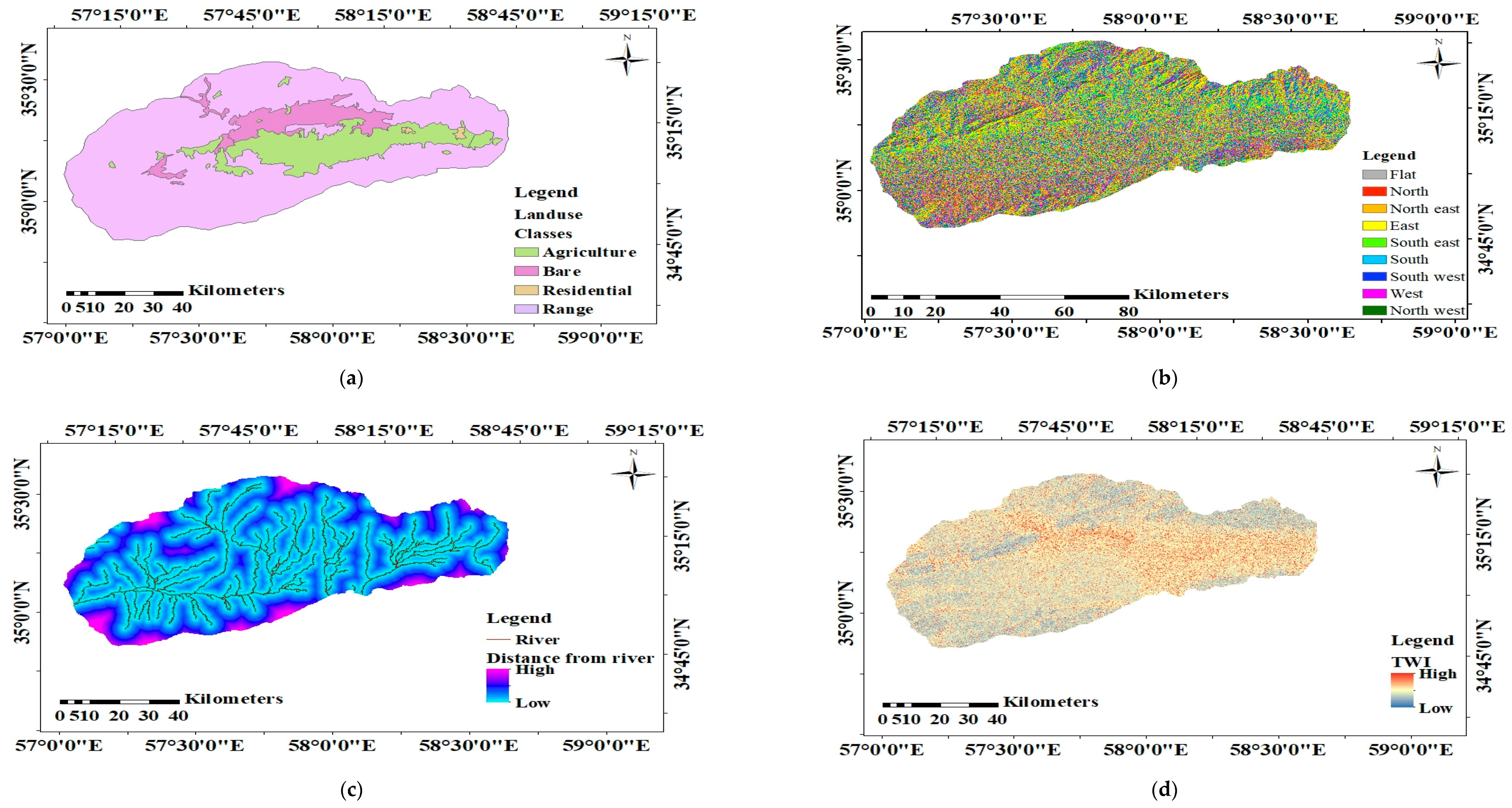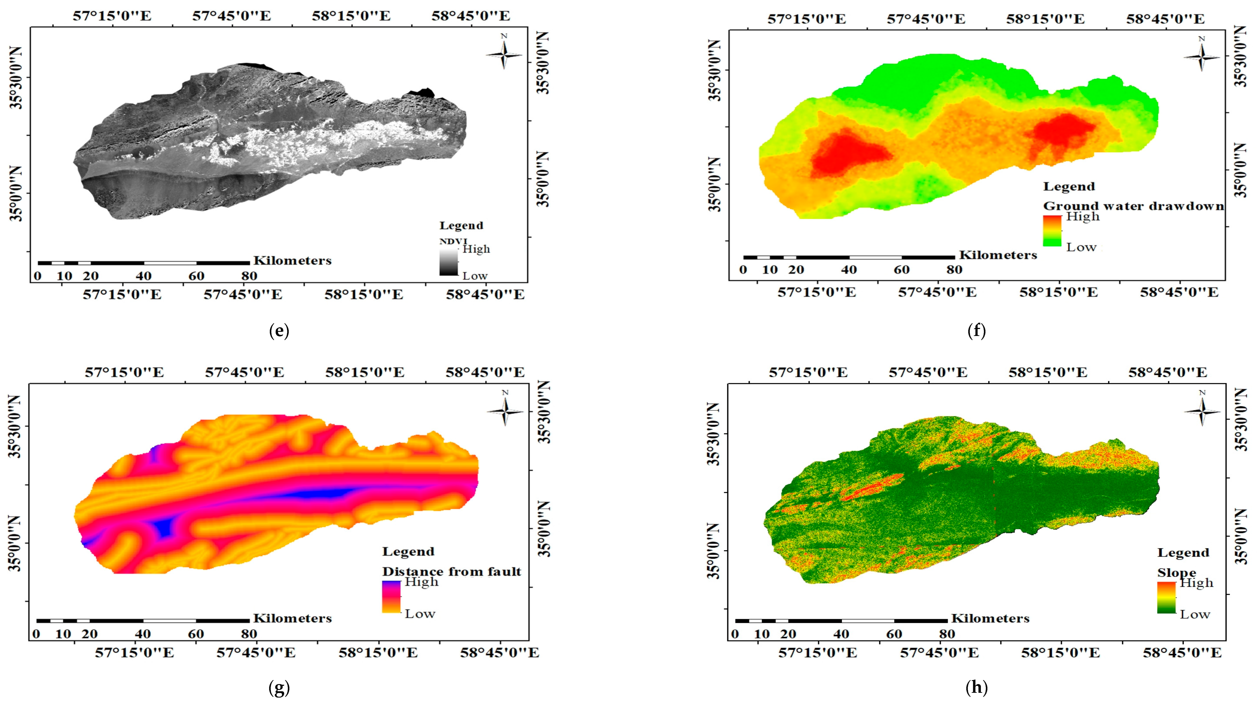We applied the methods to two study areas, Semnan Plain and Kashmar Plain in Iran, both of which have experienced severe LS in recent decades [16,17,18,19,20,21,22,23,24], using nine input variables: distance from the river, distance from the fault, groundwater drawdown, slope, aspect, land use, lithology, topographic wetness index (TWI), and normalized difference vegetation index (NDVI).

These seven MLAs were selected for analysis based on their performance merits and previous studies [16,17,18,19,20,21,22,23,24,25,26,27]. The CART approach can handle missing values in the training dataset and is insensitive to outliers since it uses surrogates [28]. The BLR approach can detect influential subsidence factors using a two-state dependent variable [29]. The SVM approach has excellent precision, robust generalization, and a higher pace of learning (REF). The BRT approach is intricate but concise, since it offers robust hydrological perception, and is thus an appropriate approach for a wide range of environmental applications. RF has higher prediction accuracy, higher efficiency when used with large datasets, low bias, and low variance by employing the bagging technique, which means that each occurrence has an equal chance of being chosen, and it avoids overfitting the data [28]. One of the advantages of LogR is its simplicity and interpretability, as the coefficients of the independent variables can be easily interpreted as the effect of each variable on the predicted probability [30]. The MLR approach is a powerful tool for modeling complex relationships between variables, as it allows analysts to examine the effect of multiple variables on a dependent variable while controlling for the effects of other variables. However, it is important to carefully consider the requirements of MLR, such as linearity, normality, and independence of errors, before applying the technique to a particular dataset.

The novel contributions of this work are comparing the ability of a broad range of classification MLAs to predict the susceptibility of an area to LS and that of a regression approach to determine the subsidence of a study area and to scrutinize the role of different factors and characteristics of a study area (e.g., amount of subsidence and data accessibility) in LS predictions, based on the outputs of these approaches.

2. Methodology

The methodology section comprises the following four main steps, as depicted in a flowchart in Figure 1:

• Preparing input variables, including slope, aspect, lithology, groundwater drawdown, distance from the river, distance from the fault, topographic wetness index, land use, and normalized difference vegetation index;
• Generating LS susceptibility maps using different MLAs (RF, CART, BLR, BRT, LogR, SVM);
• Estimating the value of LS using MLR;
• Evaluating the performance of the MLAs based on mean square error (MSE), Receiver Operating Characteristic (ROC) curve, and accuracy (AUC) of each algorithm.

2.1. Data Gathering

To prepare the input variables, Sentinel-1 satellite images of the study areas for 2015–2017 were obtained, and the locations and dimensions of several subsidence points in the areas were extracted using image analysis and by referring to technical reports (obtained from the Geological Survey and Mineral Exploration Institute) and previous studies [16,17,18,19,20,21,22,23,24,25,26,27,28,29,30,31]. The geographic location of the occurrence and the non-occurrence LS points (provided by the Geological Survey and Mineral Exploration Institute, the abovementioned studies, and RS-GIS-based methods) are used to obtain LS maps. A 12.5 m Digital Elevation Model (DEM) map was then downloaded from the ALOS PALSAR satellite, and changes in groundwater drawdown were calculated using Grace and GLADAS satellite images and observational data. Landsat-8 images were used to calculate NDVI and land use, and 1:100,000 lithology maps of the study areas were acquired from the Geological Survey of Iran. Finally, raster layers (12.5 m) were prepared and generated for the input variables.

2.2. Input Data Preparation

Input variables to the MLAs comprised slope, aspect, distance from the river, distance from the fault, NDVI, lithology, land use, and groundwater drawdown. Slope, aspect, distance from the river, and distance from the fault were derived from the DEM map. A TWI map showing topographic control over hydrological processes was derived based on DEM, flow direction, flow accumulation, and slope maps [32] using the following equation:

$$\mathrm{T}\mathrm{W}\mathrm{I}=\mathrm{l}\mathrm{n}\left(\frac{\alpha }{\tan \beta }\right)$$

(1)

where $\alpha$ is the cumulative up-slope area at any given point and $\tan \beta$ is the slope angle at that point.

The land use maps and NDVI were also obtained by processing Landsat-8 satellite images. NDVI, which represents the vegetation cover in a given area, is calculated using the following equation [33]:

$$\mathrm{N}\mathrm{D}\mathrm{V}\mathrm{I}=\frac{\mathrm{B}\mathrm{a}\mathrm{n}{\mathrm{d}}_4-\mathrm{B}\mathrm{a}\mathrm{n}{\mathrm{d}}_3}{\mathrm{B}\mathrm{a}\mathrm{n}{\mathrm{d}}_4+\mathrm{B}\mathrm{a}\mathrm{n}{\mathrm{d}}_3}$$

(2)

where $\mathrm{B}\mathrm{a}\mathrm{n}{\mathrm{d}}_4$ and $\mathrm{B}\mathrm{a}\mathrm{n}{\mathrm{d}}_3$ are the near-infrared and red bands, respectively.

To have a better perspective on the groundwater status of the study areas, data from the GRACE satellite were used to estimate total water storage (TWS) changes in the study areas. To quantify groundwater storage (GWS), values for surface storage, including soil moisture distribution, snow depth water equivalent, canopy water evaporation, and river water storage obtained from Global Land Data Assimilation System-Common Land Model (GLDAS) values were subtracted from the GRACE data. Finally, ΔGWS was computed as follows [34]:

$$∆\mathrm{G}\mathrm{W}\mathrm{S}=∆\mathrm{T}\mathrm{W}\mathrm{S}-∆\mathrm{G}\mathrm{L}\mathrm{D}\mathrm{A}\mathrm{S}$$

(3)

The groundwater drawdown was calculated using the data of observational wells obtained from the Iran Water Resources Management Company (IWRMC), and groundwater drawdown maps were generated using the IDW (Inverse Distance Weight) geostatistical method.

To avoid overfitting in machine learning approaches, one of the widely accepted methods is to randomly split the data into training and test sets [34]. Hence, of the data gathered for the study areas, around 70% was allocated randomly to model land subsidence susceptibility, while the remaining 30% was set aside to validate the model [35].

2.3. Spatial Modeling Using MLAs

2.3.1. Boosted Regression Tree (BRT)

Boosted regression tree is a nonparametric ensemble hybrid of two approaches: decision tree and boosting. The main concept in BRT involves fitting several decision trees repetitively to enhance the accuracy of the results [36,37]. Decision trees associate a response to their predictors by recursive binary splits, while boosting approaches fit several models to predictors and identify the best model to achieve more accurate results using a random subset of all data. All random subsets have the same amount of data points and are selected from the complete dataset. Data used at each tree are returned to the entire dataset and can be selected in subsequent trees, as opposed to the single models used in conventional regression approaches [38]. Finally, the boosting procedure assigns varying degrees of importance to the subsets, and subsets with the lowest prediction performance are given more weight in the next split. In this approach, predictors and inventories are allowed contribute to the modeling process over several trees, improving overall model performance [39]. The use of multiple trees in BRT eliminates the most evident drawbacks of single-tree approaches, such as comparatively poor predictive accuracy. Moreover, BRT approaches can predict various variable types (e.g., continuous and categorical data) to fit complex non-linear data and do not require data pre-processing. Since the BRT approach is based upon combining and averaging several models and modifying the dataset in each step, it has a lower error rate and higher accuracy, which is of great importance in detecting environmental phenomena like subsidence. Moreover, boosted regression trees (BRTs) showcase notable advantages, including excelling in predictive performance, adeptly handling complex data relationships, and demonstrating resilience against overfitting. However, it is important to note potential drawbacks, including computational expenses, sensitivity to noise, and the need for meticulous tuning of multiple hyperparameters. For more detailed information on the performance of BRT, see Elith et al. [39].

2.3.2. Classification and Regression Tree (CART)

Classification and regression tree is a nonparametric approach that expands a decision tree using a binary classification strategy. It recursively divides the dataset into several subsets until it forms homogeneous groups according to a modeler-specified threshold [40]. CART works with a wide variety of inputs, including numerical data, categorical data, and binary data, and its predictions are immune to monotone transformations and different scales of measurement between variables [40,41]. The inherent qualities of the CART algorithm, such as its robustness to outliers and its ability to effectively handle missing values in the training data set, can be highly advantageous in LS modeling. Also, being prone to overfitting and a lack of global optimization are the disadvantages of this approach [40].

2.3.3. Random Forest (RF)

Random forest is a commonly used MLA for various purposes, from categorization and cluster analysis to regression [42]. Breiman [28] first developed RF based on bootstrap aggregation (i.e., bagging, a method to reduce variance within a noisy dataset). The RF approach consists of three parameters: node size, number of trees, and number of features sampled. It comprises several tree-based classifiers (i.e., CARTs), each of which is built using a training set of samples (i.e., bootstrap samples) and a random variable [28]. Out-of-bag observations (OOBs) are used in RF, in which each bootstrap sample sets aside approximately one-third of the data. An estimate of the generalization error (OOB error) can be used to weigh the significance of the input variables, which are then used to identify the most influential factors on the dependent variable. RF selects the splitting variable from a random group of input variables to reduce the correlation between trees and improve model efficiency. It predicts the unseen dataset as the average of predictions from each tree once all the trees have been generated. Due to its higher accuracy in spatial modeling and better capabilities of determining the weights (i.e., importance) of different variables compared to statistical models, RF is one of the widely used MLAs in studying LS. Random forest (RF) offers robustness against overfitting, effective handling of missing values, and capability to manage a large number of features. Nevertheless, it is essential to consider potential downsides, such as computational expenses, potential suboptimal performance on highly noisy data, and a trade-off in interpretability compared to simpler models [31]. More information on RF can be found in Breiman [28].

2.3.4. Support Vector Machine (SVM)

Support vector machine was first developed by Cortes and Vapnik [43] for classification purposes. SVM is a type of MLA that uses kernel functions and hyperplanes to convert non-linear problems into linear problems that can be handled more easily [44,45,46]. It tries to minimize the upper bound of the generalization error, as opposed to the training error. Moreover, SVM seeks a global optimum under conditions that can be easily met, rather than identifying the local minimum. The better classification abilities of the SVM algorithm for environmental data and using optimal data separation techniques make SVM more suitable for environmental studies such as subsidence susceptibility [11]. SVM exhibits strength in high-dimensional spaces, demonstrating effectiveness, robustness in handling outliers, and versatility with various kernel functions. However, it is essential to acknowledge their computational intensity, interpretational challenges, and sensitivity to the choice of kernel and hyperparameters, aspects that should be carefully considered in practical applications. For more detailed information on SVM, see Marjanovic et al. [47].

2.3.5. Bayesian Logistic Regression (BLR)

Bayesian logistic regression, one of the most popular classification MLAs, is a generalized linear approach where the probability of success can be expressed as a sigmoid function (for binary classification). When analyzing the relationship between the dependent and independent variables, BLR follows three steps: (i) determining each parameter’s initial probability, (ii) finding the likelihood function of the data, and (iii) making a posterior distribution function for parameters [33]. The underlying concept is that a Bernoulli distribution is assumed for the values (i.e., 0 and 1) forecast by a linear combination of predictors, which are mapped to the probability value by the logistic function [48]. By integrating Bayesian techniques with a logistic regression model and employing uncertainty estimation approaches, more robust outcomes can be obtained and mitigate the risk of overfitting the data [49]. This can be particularly advantageous for spatial mapping objectives. Also, Bayesian logistic regression (BLR) holds advantages in providing probabilistic outputs, adeptly managing multicollinearity, and offering interpretability. However, it is crucial to acknowledge potential limitations, including the assumption of linearity in relationships, potential challenges in capturing complex patterns in data, and sensitivity to outliers. For more information on BLR, see Pavlyshenko [48].

2.3.6. Logistic Regression (LogR)

Logistic regression is a statistical approach for analyzing the relationship between a dependent variable and one or more independent variables, where the dependent variable is categorical (i.e., binary or ordinal), and the independent variables can be continuous, categorical, or a combination of both. LogR aims to model the probability of a certain outcome or event based on the values of the independent variables. The output of LogR is a predicted probability of the dependent variable belonging to a particular category. LogR fits a logistic function to the data, a sigmoid-shaped curve that maps any input value to a value between 0 and 1. The logistic function takes the following form [30]:

$$\mathrm{p}=\frac{1}{(1+{\mathrm{e}\mathrm{x}\mathrm{p}}^{-\mathrm{z}})}$$

(4)

where p is the predicted probability of the dependent variable, z represents the linear combination of the independent variables and their coefficients, and exp denotes the exponential function.

The Log R approach estimates the coefficients of the independent variables that best fit the data, and these coefficients are then used to calculate the predicted probabilities of the dependent variable [50]. The response variables of the logistic regression model can be binary or multilevel classes, and the predictor variables can be a combination of continuous, discrete, or binary variables. In addition, LogR does not require data to be normal, making it particularly useful in environmental studies. However, the increased likelihood of data overfitting is a drawback of this method [11].

2.3.7. Multiple Linear Regression (MLR)

Multiple linear regression is a statistical method that uses numerous variables to predict the outcome of a response variable. The purpose of MLR analysis is to simulate the linear connection between the independent factors and the dependent variable, since dependent variables are affected by numerous factors in most real-world issues [50]. Due to the inclusion of additional explanatory variables, MLR can be viewed as an extension of ordinary least-squares (OLS) regression of the form suggested by Chakraborty et al. [51]:

$$\mathrm{y}={\mathrm{b}}_0+{\mathrm{b}}_1{\mathrm{x}}_1+{\mathrm{b}}_2{\mathrm{x}}_2+\cdots +{\mathrm{b}}_{\mathrm{n}}{\mathrm{x}}_{\mathrm{n}}+\mathsf{\epsilon }$$

(5)

where y represents the dependent variable; ${\mathrm{x}}_1$, ${\mathrm{x}}_2$, …, ${\mathrm{x}}_{\mathrm{n}}$ are the independent variables; $b_0$ denotes the intercept; ${\mathrm{b}}_1$, ${\mathrm{b}}_2$, …, ${\mathrm{b}}_{\mathrm{n}}$ are the regression coefficients; and $\mathsf{\epsilon }$ is the error term. The regression coefficients represent the change in the dependent variable for a one-unit increase in the corresponding independent variable, while all other independent variables are assumed to be constant.

To perform MLR, the data analyst must first collect data on the dependent and independent variables and then use these data to estimate the regression coefficients, using a technique such as least square regression. The analyst can then use the estimated coefficients to predict the value of the dependent variable for new values of the independent variables.

2.4. Validation of the LS Susceptibility Maps

The purpose of validation in any modeling process is to determine whether the developed model produces sufficiently accurate results for the intended aim [52,53].

In the present analysis, AUC (also known as accuracy or efficiency), ROC curve, F-1 score, and MSE were used to evaluate the performance of the different MLAs for the two study areas and datasets. AUC is a statistical measure of how well a model detects or excludes conditions and is measured for any model as follows:

$$\mathrm{A}\mathrm{U}\mathrm{C}=\frac{\mathrm{T}\mathrm{P}+\mathrm{T}\mathrm{N}}{\mathrm{T}\mathrm{P}+\mathrm{T}\mathrm{N}+\mathrm{F}\mathrm{P}+\mathrm{F}\mathrm{N}}$$

(6)

where TN, FN, TP, and FP denote the true negative, false negative, true positive, and false positive values, respectively. TP and TN represent the number of pixels correctly identified, whereas FP and FN represent the number of pixels incorrectly categorized [49,50,51,52,53,54,55].

Although there is no general rule for choosing a cut-off value for predicting natural hazards, researchers have frequently considered probability (P) values greater than 0.5 to indicate unreliable results [56,57]. Therefore, we selected a probability of 0.50 as the threshold, so a cell with P > 0.5 and LS was categorized as TP. FP (error type I) indicates that a cell without LS is classed as unstable (P > 0.5), whereas FN (error type II) indicates that a cell with LS is classified as stable (P < 0.5).

The ROC curve which plots sensitivity (Y-axis) against 1-specificity (X-axis) and F1 − score are also good measures to investigate the performance of MLAs. The following equations are used to plot the ROC curve and calculate the F1 − score.

$$\mathrm{s}\mathrm{e}\mathrm{n}\mathrm{s}\mathrm{i}\mathrm{v}\mathrm{i}\mathrm{t}\mathrm{y}=\frac{\mathrm{T}\mathrm{p}}{\mathrm{T}\mathrm{p}+\mathrm{F}\mathrm{N}}$$

(7)

$$\mathrm{s}\mathrm{p}\mathrm{e}\mathrm{c}\mathrm{i}\mathrm{f}\mathrm{i}\mathrm{c}\mathrm{i}\mathrm{t}\mathrm{y}=\frac{\mathrm{T}\mathrm{N}}{\mathrm{T}\mathrm{N}+\mathrm{F}\mathrm{P}}$$

(8)

$$\mathrm{P}\mathrm{e}\mathrm{r}\mathrm{c}\mathrm{i}\mathrm{s}\mathrm{i}\mathrm{o}\mathrm{n}=\frac{\mathrm{T}\mathrm{p}}{\mathrm{T}\mathrm{p}+\mathrm{F}\mathrm{P}}$$

(9)

$$\mathrm{R}\mathrm{e}\mathrm{c}\mathrm{a}\mathrm{l}\mathrm{l}=\frac{\mathrm{T}\mathrm{p}}{\mathrm{T}\mathrm{p}+\mathrm{F}\mathrm{N}}$$

(10)

$$\mathrm{F}1-\mathrm{s}\mathrm{c}\mathrm{o}\mathrm{r}\mathrm{e}=\frac{2(\mathrm{P}\mathrm{e}\mathrm{r}\mathrm{c}\mathrm{i}\mathrm{s}\mathrm{i}\mathrm{o}\mathrm{n}\times \mathrm{R}\mathrm{e}\mathrm{c}\mathrm{a}\mathrm{l}\mathrm{l})}{(\mathrm{P}\mathrm{e}\mathrm{r}\mathrm{c}\mathrm{i}\mathrm{s}\mathrm{i}\mathrm{o}\mathrm{n}+\mathrm{R}\mathrm{e}\mathrm{c}\mathrm{a}\mathrm{l}\mathrm{l})}$$

(11)

Mean squared error is a popular metric to evaluate the performance of a model. In simple terms, MSE measures how well a model can predict a variable by calculating the average squared difference between predicted and actual values. The squared differences are used instead of absolute differences to ensure that positive and negative errors do not cancel each other out. MSE is calculated as follows [58,59]:

$$\mathrm{M}\mathrm{S}\mathrm{E}=\frac{1}{\mathrm{n}}\sum {{(\mathrm{y}}_{\mathrm{i}}-\widehat{{\mathrm{y}}_{\mathrm{i}}})}^2$$

(12)

where n is the number of observations, and ${\mathrm{y}}_{\mathrm{i}}$ and $\widehat{{\mathrm{y}}_{\mathrm{i}}}$ represent the actual and predicted values of the variable, respectively.

The MSE value ranges from 0 to infinity, with 0 indicating perfect prediction and higher values indicating poorer performance. The model with the lowest MSE value is considered the best fit for the data. MSE has several advantages over other metrics, including its ability to penalize large errors more severely than small errors, making it more sensitive to outliers.

3. Study Areas

In recent decades, the intensification of agriculture, urbanization, and excessive water withdrawal have caused irreversible environmental changes, including LS, in Iran. Subsidence has been observed in many cities, including Tehran, Isfahan, and Ahvaz, due to unsustainable water management. In this study, we scrutinized the performance of different MLAs in identifying LS-prone zones in two of Iran’s important but less addressed areas (Semnan Plain and Kashmar Plain) (Figure 2a), which have experienced a continuous drop in groundwater level in recent decades. The primary rationale behind selecting these two regions stems from the notable occurrence of subsidence in both areas. The decision is influenced by the proximity of lithological characteristics in these regions, coupled with similar trends in groundwater drawdown and the comparable nature of the land use. Consequently, it is of significant importance to employ various machine learning algorithms for the comparative analysis of subsidence in these two regions. LS has been occurring in both areas for some decades and has caused a drastic reduction in land elevation. In Kashmar Plain, LS has caused some areas to sink by more than 22 cm annually, leading to infrastructure destruction, increased flooding, and water supply disruption [16]. In addition, LS has caused damage to agricultural land, resulting in economic losses for farmers. Semnan Plain has also been affected by LS of approximately 12 cm/year [17]. As a result, the identification of areas that are vulnerable to LS can be highly useful for the management and prevention of further LS and the destructive processes that are linked with subsidence.

3.1. Semnan Plain

Semnan Plain is located in the western part of Semnan province in Iran, on the southern foothills of the Alborz Mountain range and northern regions of the Kavir desert (Figure 2b). It has an approximate area of 1200 km² and lies between a longitude of 53°3′ and 53°40′ E and a latitude of 35°18′ and 35°43′ N [60]. The elevation ranges from 874 m above sea level (masl) adjacent to desert areas to 1857 masl in mountainous regions. According to previous studies and geological maps of the area, the common soil type in the middle of the plain, around Semnan City and its surroundings, is young alluvial sediment [61]. The lithological characteristics of Semnan Plain, which is located in a tectonically active region, are presented in

Table 1. The lithology of Semnan plain.

Code	Description	Area (%)
Qft2	Low-level sediment fan and valley terrace deposits	59.4
Mur	Sandy marl	21.2
Qft1	High-level piedmont fan and valley terrace deposits	10.3
Eav	Dacitic to Andesitic volcanic	3.26
Ek	Shale with tuff intercalations	2.34
TRJs	Dark grey shale and sandstone	2.03
Qd	Darjazin fan deposits	2.01

. Geomorphological surveys of the area indicate that the slope of the plain is from north to south and that seasonal flows enter the plain from the northern and northeastern highlands [62]. The dominant land uses in the area are rangeland and agriculture. Semnan Plain has a semi-arid cold to cold-arid climate [63]. Mean annual precipitation mainly consists of rainfall and is about 130 mm, and the mean annual temperature is around 16.1 °C [31]. Groundwater extraction has significantly increaed in recent years due to low precipitation, high sedimentation, scarce surface water, and improper water management, in order to meet the needs of various sectors such as the municipal, agricultural, and industrial sectors. This has led to a drastic decline in groundwater levels in the region and associated environmental, social, and economic issues. The groundwater decline has been most severe in the eastern and southern parts of Semnan Plain as a result of the higher intensity of agriculture practices in these regions [60]. Figure 3 shows land use, aspect, distance from the river, TWI, NDVI, distance from fault, groundwater drawdown, and slope maps for Semnan Plain.

3.2. Kashmar Plain

Kashmar Plain covers an area of 6467 km² and is located in the western part of Khorasan Razavi province in Iran, between a longitude of 57°10′ and 58°35′ E and a latitude of 34°45′ and 35°30′ N [25] (Figure 2c). The elevation ranges between 782 and 2259 masl. Like Semnan Plain, Kashmar Plain mainly consists of rangeland and agricultural land. A large desert fault (Droneh) is located along the northern border of the Kashmar plain, and its internal trend is east–west [64]. The plain receives a mean annual precipitation of 156 mm, mainly in the form of rainfall, and has a mean annual temperature of around 17.5 °C [64]. In terms of climate, the region is classified as semi-arid to arid. Since no permanent rivers exist in the area, the water supply depends upon groundwater resources, with 84% of withdrawn groundwater used for irrigation, 9% in the municipal sector, and the rest for industrial and other purposes [65]. A recent groundwater balance analysis reported 76 MCM over-exploitation per year from the aquifer [24]. The distribution of LS in Kashmar Plain is not uniform, and the sunken areas are mostly evident as a cluster of sinkholes varying in width and depth through the plain. The lithological characteristics of Kashmar Plain are presented in

Table 2. The lithology of Kashmar plain.

Code	Description	Area (%)
Qft2	Low level sediment fan and valley terrace deposits	56.9
Mur	Sandy marl	7.52
Qft1	High-level piedmont fan and valley terrace deposits	7.13
Eav	Dacitic to Andesitic volcanic	13.36
Qsf	Lowest alluvial deposits	7.34
TRJs	Dark grey shale and sandstone	4.03
Sr	serpentinite	2.06

. Figure 4 depicts land use, aspect, distance from the river, TWI, NDVI, distance from the fault, groundwater drawdown, and slope maps of Kashmar plain.

4. Results

Land subsidence in the two study areas (Semnan Plain and Kashmar Plain) was calculated separately using the six classification-based approaches and one regression-based MLA described in the Section 2.

4.1. Analysis of Variable Importance and Correlation

Table 3. The correlation between input variables of Semnan Plain.

	Groundwater Drawdown	Distance from the River	NDVI	Distance from the Fault	TWI	Slope
Groundwater drawdown	1	0.76	0.51	0.41	0.82	0.26
Distance from the river	0.76	1	0.29	0.48	0.85	0.65
NDVI	0.51	0.29	1	0.19	0.87	0.32
Distance from the fault	0.41	0.48	0.32	1	0.1	0.15
TWI	0.82	0.85	0.87	0.1	1	0.22
Slope	0.26	0.65	0.32	0.15	0.22	1

and

Table 4. The correlation between input variables of Kashmar Plain.

	Groundwater Drawdown	Distance from the River	NDVI	Distance the from Fault	TWI	Slope
Groundwater drawdown	1	0.81	0.57	0.43	0.84	0.22
Distance from the river	0.81	1	0.33	0.53	0.87	0.69
NDVI	0.55	0.33	1	0.17	0.89	0.37
Distance from the fault	0.46	0.53	0.17	1	0.15	0.18
TWI	0.84	0.87	0.89	0.15	1	0.27
Slope	0.22	0.69	0.37	0.18	0.27	1

present the correlation between input variables for Semnan and Kashmar plains, respectively. According to the obtained results, the BRT, SVM, and RF approaches demonstrated better performance in predicting susceptibility to LS among the six studied approaches, as they had the lowest error rate.

Figure 5 illustrates the relative importance of the input variables for the top three approaches in the study areas. According to the BRT approach, variables playing the most significant role in LS in Semnan Plain were groundwater drawdown (20.31%), distance from the river (17.11%), land use (14.98%), NDVI (12.75%), and lithology (11.93%), while distance from the fault (9.51%), TWI (7.32%), and slope (6.11%) were less important for predicting LS. According to the SVM approach, the factors with the greatest impact on subsidence in Semnan Plain were groundwater drawdown (31.21%), distance from the river (16.01%), land use (13.18%), NDVI (10.15%), and lithology (9.43%), with distance from the fault (8.51%), TWI (6.12%), and slope (5.31%) having less impact. In the RF approach, there was an even stronger correlation between groundwater drawdown (33.21%), distance from the river (15.21%), land use (12.78%), NDVI (9.75%), and lithology (9.03%) and LS in Semnan plain, while distance from the fault (8.51%), TWI (6.12%), and slope (5.01%) had minor impacts (Figure 5a).

According to the BRT approach, the three most important factors in LS in Kashmar Plain were groundwater drawdown (35.31%), distance from the river (23.1%), and land use (12.98%), while NDVI (9.66%), lithology (9.5%), distance from the fault (8.5%), TWI (7.3%), and slope (6.1%) played minor roles. The SVM approach also identified groundwater drawdown (41.51%), distance from the river (21.31%), and land use (10.90%) as the three most important factors for LS in Kashmar Plain, while NDVI (7.5%), lithology (7.15%), distance from the fault (5.95%), TWI (4.33%), and slope (3.13%) had weaker correlations with LS. In addition, the RF approach identified groundwater level (44.31%), distance from the river (20.51%), and land use (10.40%) as the three most influential factors for LS in Kashmar Plain, while NDVI (4.95%), lithology (5.63%), distance from the fault (4.95%), TWI (4.33%), and slope (3.13%) played less significant roles (Figure 5b).

4.2. Land Subsidence Susceptibility Mapping

Areas prone to LS were predicted by extracting weights from the BRT, SVM, and RF approaches and mapping them in ArcGIS. Land subsidence was classified into four groups (very high, high, medium, and low) using the natural break method (for more information on this method, see Abdollahi et al. [66]). Figure 6 presents the subsidence susceptibility map generated by BRT (best) and LogR (worst) for both study areas. According to Figure 6b, it is clear that BRT achieved better performance in predicting LS. Both BRT and LogR predicted very high levels of LS in central areas of Semnan Plain, but BRT performed better than LogR in predicting areas with high subsidence. LogR performed weakly in distinguishing areas with high and medium subsidence.

The BRT and LogR approaches detected areas with very high subsidence in the southeast and northwest of Kashmar Plain. However, the LogR approach showed weakness in distinguishing areas with low and moderate LS and classified most of the areas with medium subsidence in the low subsidence category. Overall, the accuracy of LS prediction was higher for Semnan Plain, which had more data points than Kashmar Plain.

4.3. Land Subsidence Prediction

According to technical reports and previous studies, the average LS rate in Semnan Plain and Kashmar Plain is approximately 12 and 22 cm/year, respectively. The MLR approach showed good performance in predicting these LS values (Figure 7), with MSE for Semnan Plain and Kashmar Plain equal to 0.25 and 0.32, respectively.

4.4. Model Validation and Comparison

The accuracies of the different models in predicting LS values for the two study areas are presented in

Table 5. Accuracy of the approaches.

Approach	AUC
	Semnan Plain	Kashmar Plain
RF	0.73	0.69
CART	0.70	0.63
BRT	0.75	0.74
SVM	0.72	0.70
BLR	0.71	0.68
LogR	0.67	0.56

. The BRT, SVM, and RF approaches yielded the more accurate responses for predicting subsidence in both Semnan and Kashmar plains. The accuracy scores for Semnan Plain were 0.75, 0.72, and 0.73 for the BRT, SVM, and RF approaches, respectively. For Kashmar Plain, the accuracy rates were 0.74, 0.7, and 0.69 for the same approaches. According to the AUC classes (i.e., poor (0.5–0.6), average (0.6–0.7), good (0.7–0.8), very good (0.8–0.9), and excellent (0.9–1)), the performance of BRT was classified as good for both regions. On the other hand, the performance of RF and SVM was classified as good for Semnan Plain and average for Kashmar Plain. In general, all the examined approaches had average to good performance in modeling LS; however, BRT was deemed to have attained better performance due to its higher accuracy in comparison to the other approaches. BRT showcases notable advantages including excelling in predictive performance, adeptly handling complex data relationships, and demonstrating resilience against over-fitting. However, it is important to note potential drawbacks, including computational expenses, sensitivity to noise, and the need for meticulous tuning of multiple hyperparameters. For more detailed information on the performance of each model, see Section 2.3.

Confusion diagrams for Semnan plain and Kashmar plain are shown in Figure 8 and Figure 9 and

Table 6. Confusion matrix for Semanan plain.

MLAs
	RF	CART	BRT	BLR	SVM	LogR
TP	58	50	60	57	57	45
TN	1	4	1	1	1	9
FP	2	4	1	1	5	1
FN	20	23	19	22	18	25

and

Table 7. Confusion matrix for Kashmar plain.

MLAs
	RF	CART	BRT	BLR	SVM	LogR
TP	11	9	11	10	10	8
TN	1	1	2	1	1	1
FP	3	5	1	3	4	5
FN	5	5	6	6	5	6

, respectively. The ROC curves and F1 − scores of each model are presented in Figure 10 and

Table 8. F1 − scores of each model.

Approach	RF	CART	BRT	BLR	SVM	LogR
Kashmar Plain	0.70	0.64	0.74	0.67	0.68	0.56
Semnan Plain	0.83	0.78	0.84	0.80	0.82	0.76

, respectively. According to Figure 10, the BRT approach outperforms the other five algorithms, with AUC values of 0.76 and 0.74 in both Semnan and Kashmar plains. Additionally, F1 − scores in Table 8 reveal that, in both study areas, the ranking of approaches according to their accuracy is as follows: BRT > RF > SVM > BLR > CART > LogR.

4.5. Discussion

4.5.1. Comparison of Applied Approaches

Modeling and simulation are useful decision support tools to better understand potential environmental hazards. The use of modeling tools also allows decision-makers to have a better understanding about modeled phenomena and plan effective environmental strategies. Utilizing machine learning models enables policymakers to delineate land subsidence-prone areas, facilitating the establishment of risk maps and zoning regulations. Urban planners can strategically avoid placing critical infrastructure or high-density developments in identified high-risk zones. For example, policymakers and urban planners can make better decisions about infrastructure projects by considering potential subsidence risks in different areas. This ensures that infrastructure is designed and located in more safe regions (i.e., non-subsidence areas), minimizing the impacts of subsidence on roads, buildings, and utilities [67]. Also, policymakers can optimize resource allocation by using machine learning findings to identify high-risk areas. This allows for targeted monitoring, implementing mitigative measures, and upgrading infrastructure, and it leads to an increase in the overall negative impacts of land subsidence.

However, a wide variety of modeling frameworks and approaches with different predictive power are available, which can result in diverse outputs. In the present study, BRT, SVM, and RF all achieved acceptable performance in predicting LS in the two study areas, Semnan Plain and Kashmar Plain in Iran, as measured by the AUC metric. Similarly, Sekkeravani et al. [11] created zoning maps for detecting areas susceptible to LS in the central plains of Iran using various models and found that RF, BRT, and SVM achieved a significant level of accuracy.

The LogR approach performed poorly compared to the other five MLAs in terms of predicting LS in the study areas, while CART and BLR showed average performance. A previous study by Hakim et al. [68] investigating the performance of four MLAs (AdaBoost, multilayer perceptron, LogR, LogitBoost) also found that LogR was the least successful approach in predicting LS susceptibility. The findings in the present study provide ample support for the claim that tree-based MLAs, particularly SVM and BRT, are adept at identifying non-linear connections with a high degree of complexity [69]. There was substantial agreement between the results obtained and those of Lee et al. [70] for the BRT and RF approaches, but no previous study had tested and compared seven distinct MLAs in the two study areas.

4.5.2. Evaluation of the Significance of Variables

Due to the location of the study areas in arid regions of Iran with low precipitation rates, groundwater is the main source of water for different demand sectors, especially agriculture. According to the BRT and RF results, the major cause of LS in both Semnan Plain and Kashmar Plain is overexploitation and mismanagement of groundwater resources. Studies in Florida (USA) have revealed similar issues, with excessive groundwater extraction being identified as the primary cause of subsidence [71]. Subsidence and ground collapse are the result of stresses and strains imposed on groundwater resources by extensive groundwater depletion, leading to a catastrophic decrease in potentiometric levels [72]. Moreover, Semnan Plain has insufficient LS provisioning and monitoring systems [73], enabling the overexploitation of groundwater resources. In addition, there has been a notable increase in population, expansion of industrial regions, and intensified water demand in Semnan Plain in recent decades [61], resulting in the unsustainable extraction of groundwater resources. Studies conducted in other areas have also revealed a significant relationship between extensive groundwater withdrawal and land subsidence. For instance, Orhan [74] scrutinized the causes of LS in Konya, Turkey, and identified a strong correlation (0.95) between LS occurrence and changes in groundwater level.

Subsidence in the two study areas has also been significantly influenced by land use, with agricultural areas in both Semnan Plain and Kashmar Plain having experienced their highest subsidence due to excessive groundwater withdrawal. Studies by Mohammady et al. [16] and Rahmati et al. [17,25] investigating LS susceptibility in the Semnan and Kashmar plains using tree-based approaches also found that some of the most severe LS occurred in agricultural areas.

The lithology of the study areas was another influential factor in LS, with soils in the low-level pediment fan and valley terrace deposits being more susceptible to subsidence. A study by Saeidi et al. [24] also found that sediment type and sediment thickness were among the primary reasons for LS in Kashmar Plain.

5. Conclusions

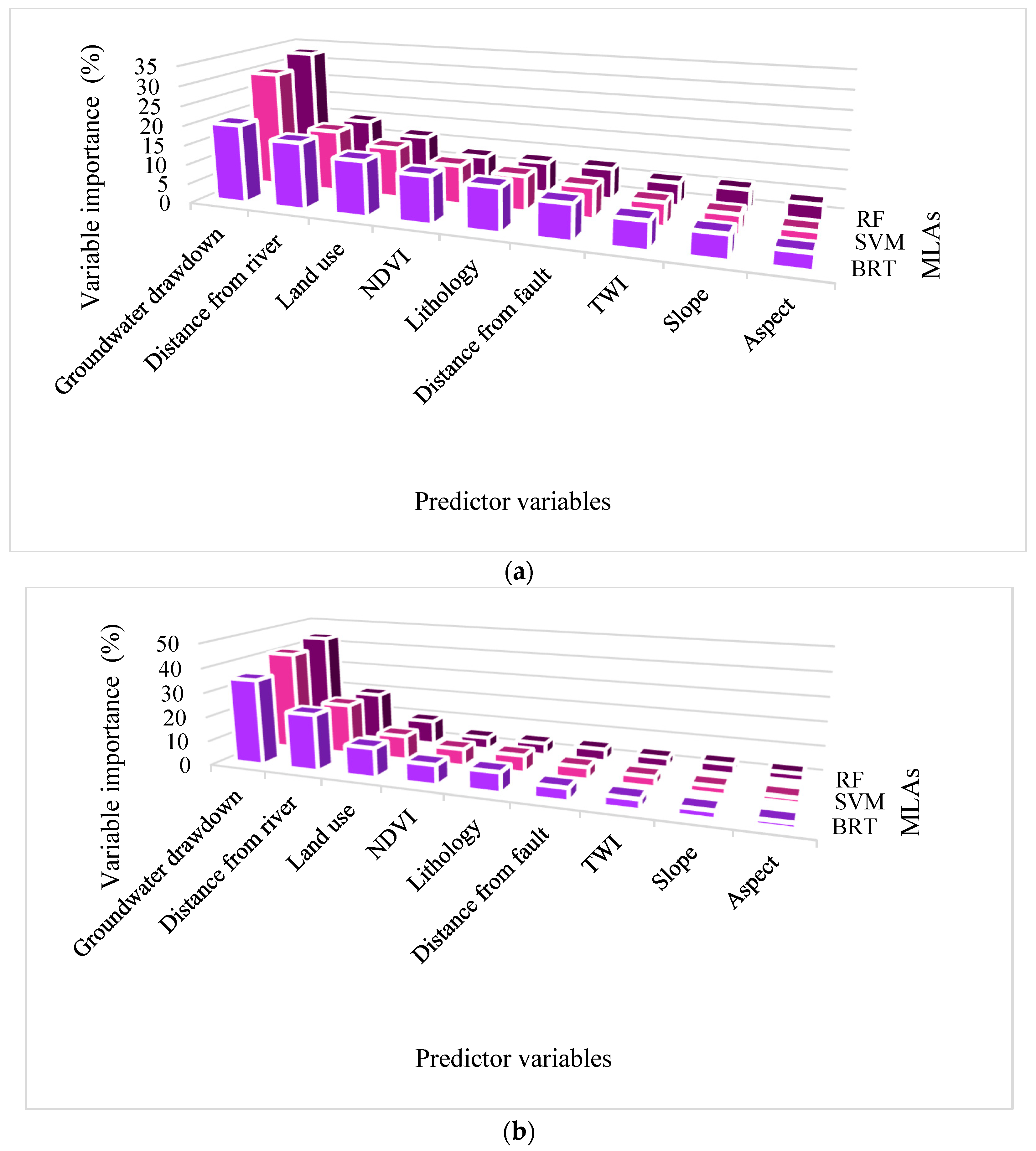
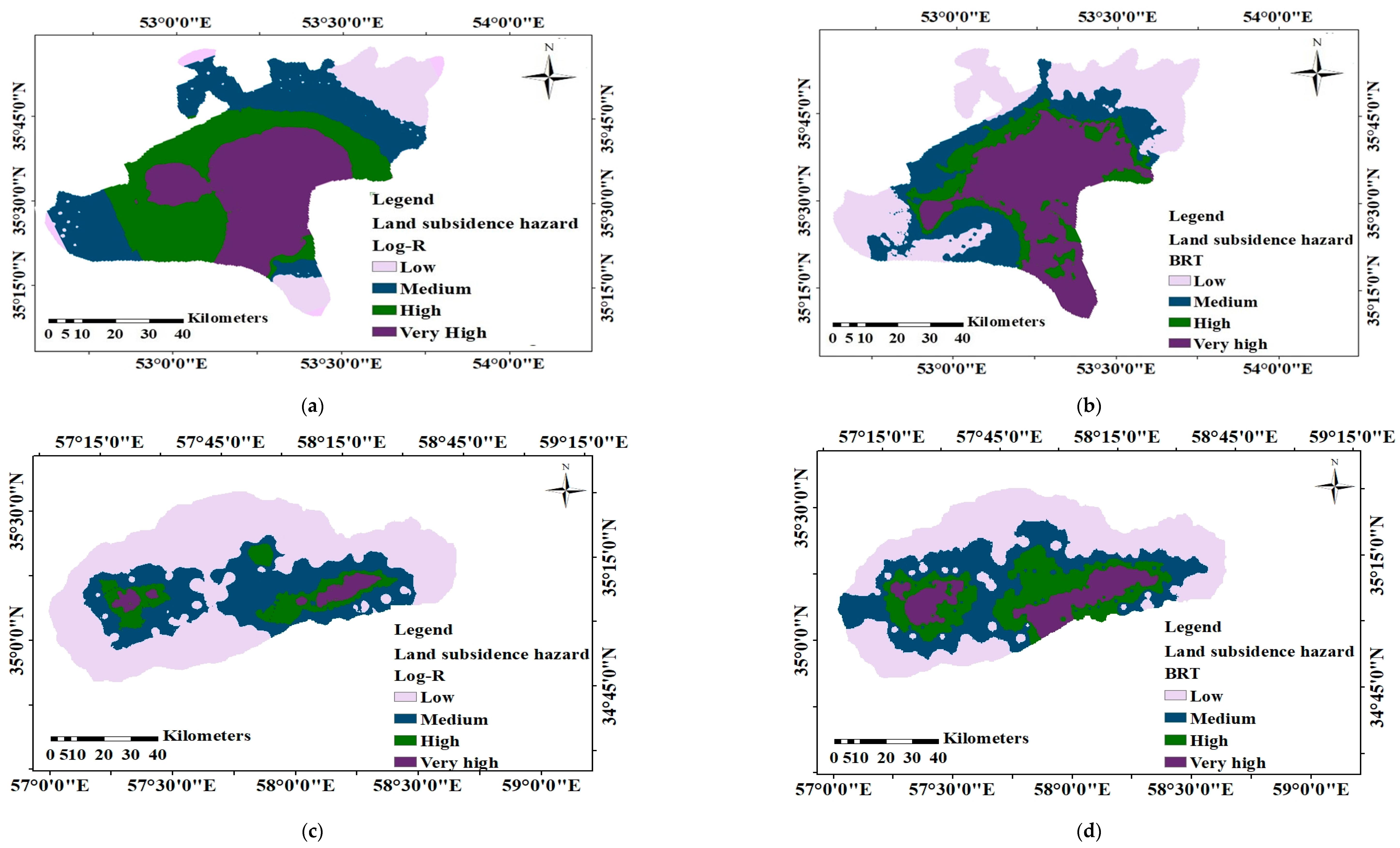
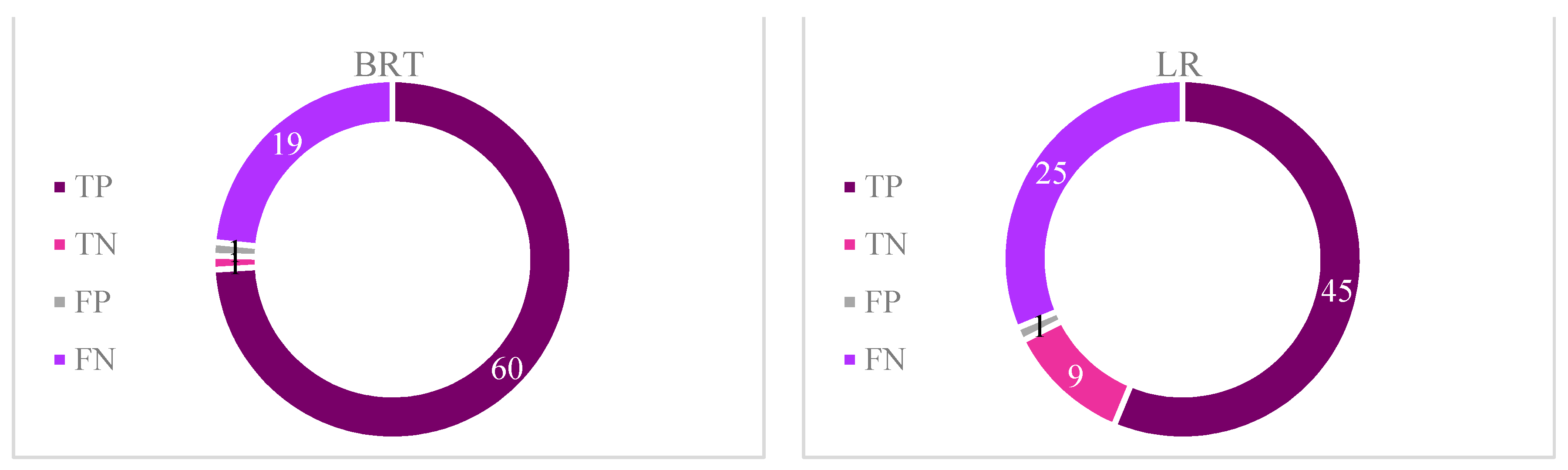
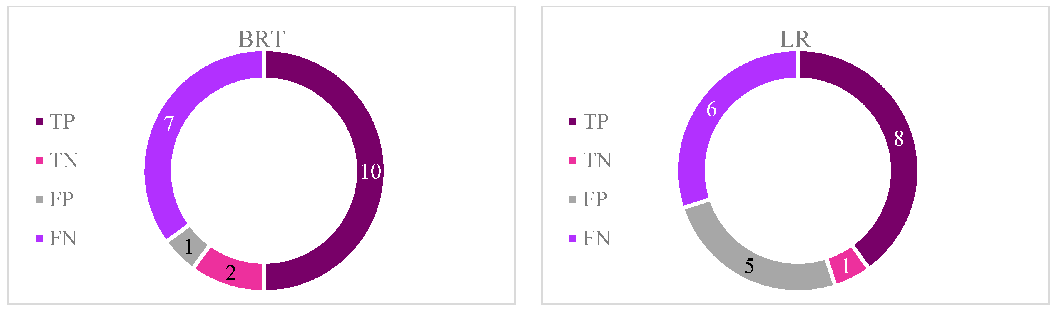
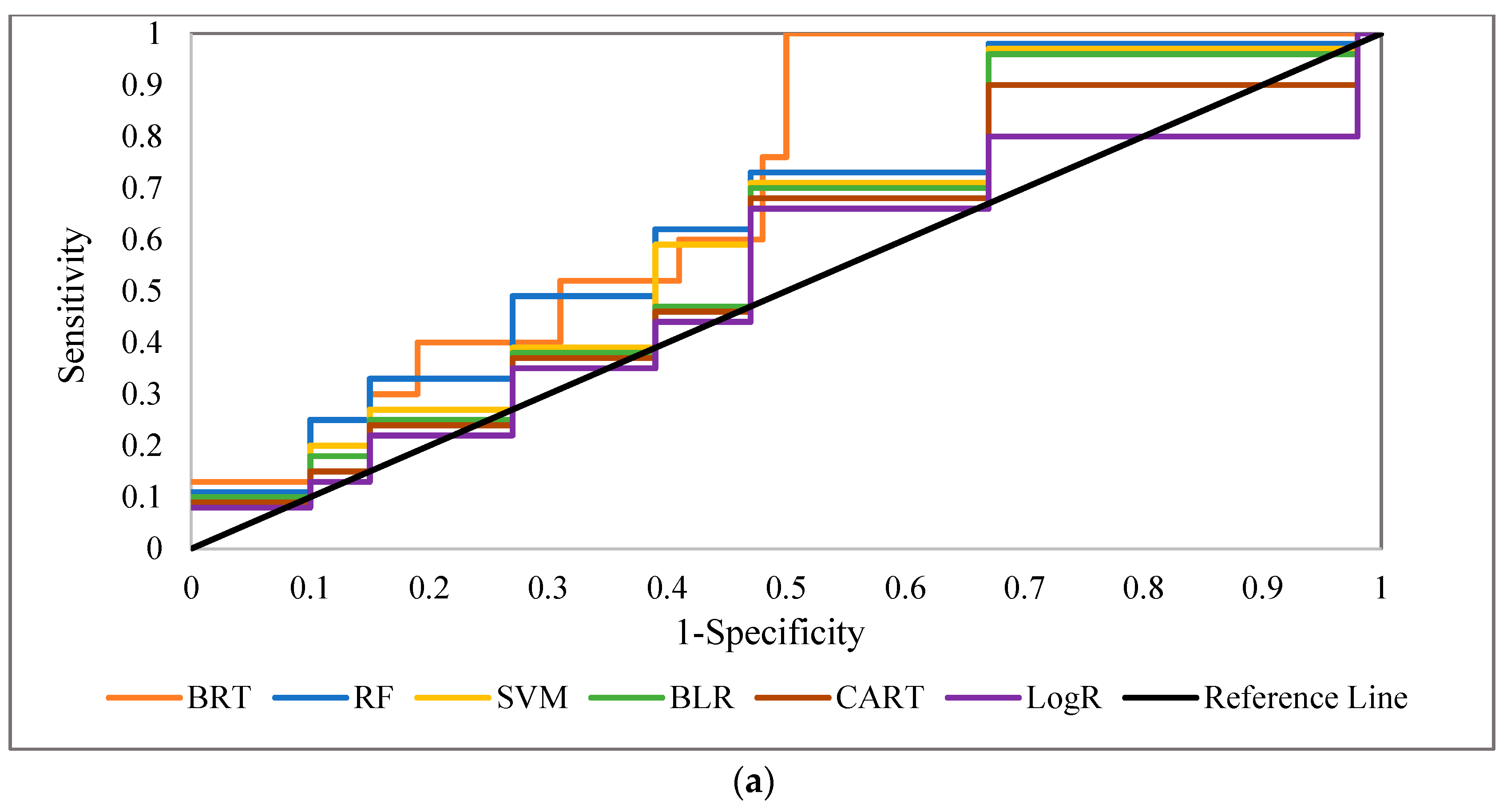
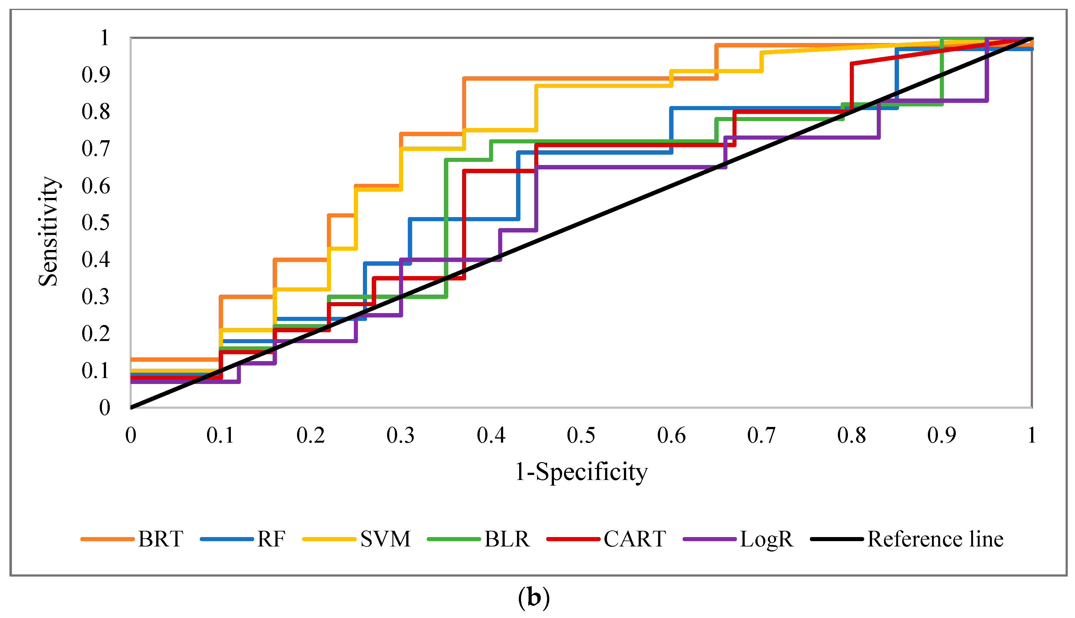
One of the detrimental natural hazards in both Semnan Plain and Kashmar Plain is land subsidence, which can result in infrastructure failure and environmental and economic issues. In this study, six classification-based MLAs (BRT, RF, SVM, BLR, CART, and LogR) were used to investigate LS in these two areas. In addition, MLR was applied to predict LS in the two areas. Lithology, slope, aspect, TWI, distance from the river, distance from the fault, land use, NDVI, and groundwater drawdown at the sites were all taken into consideration in LS modeling. The BRT approach was able to predict LS hazard in both study areas with a good degree of accuracy, while RF and SVM also showed good performance for both areas. The LogR approach showed the worst performance in predicting LS in both study areas. Overall, the results indicated that LS in both areas is mainly occurring due to groundwater drawdown, but that the distance from the river, NDVI, land use, and lithology also have significant impacts.

According to the results, groundwater drawdown is one of the most influential factors responsible for LS in the study areas. Typically, one answer in such situations is to carry out water transfer projects to offer alternate resources for local communities. Due to the risks and high implementation costs of such projects, they are not advised for providing alternate water resources. Improving water management across various sectors, utilizing water purification techniques by industries to prevent water pollution, and enacting laws regulating water usage in different demand sectors (e.g., municipal, industrial, agriculture) can aid in replenishing water resources. Furthermore, implementing projects aiming at reducing water consumption in agricultural sectors such as utilizing modern irrigation techniques (e.g., drip and rain irrigation methods), cultivating crops with higher resilience to water scarcity, close monitoring of groundwater level, and prohibiting illegal groundwater extraction can hinder the further overexploitation of resources.

In this study, land subsidence was investigated between the years 2015 and 2017. Access to more updated temporal data can enhance the accuracy of results. The primary limitation of the current study stems from the unavailability of subsidence rate data in the region. The absence of such data prevents a comprehensive analysis of the gradual influence of various factors on land subsidence over time, hindering the ability to simulate real-time possibilities of subsidence. Utilizing the interferometric synthetic aperture radar (InSAR) time series analysis technique could address this limitation. Therefore, it is recommended that future research explores the use of subsidence rate as a response variable in predicting land subsidence susceptibility using machine learning models, contingent upon the availability of relevant datasets.

Furthermore, certain critical factors, such as sedimentation rate, altitude, soil type, and curvature, were not considered in this study. Incorporating these factors into the prediction process in future studies is crucial for obtaining more accurate results. The inclusion of such data can significantly enhance the precision of the outputs.

Furthermore, there is potential for future studies to focus on developing a practical risk framework. This framework could incorporate vulnerability components, integrating data on assets and populations susceptible to the impacts of land subsidence. While these tasks hold significant value for addressing real-world land subsidence challenges, they necessitate further investigation that includes the acquisition of relevant datasets. This not only applies to the present study regions but also extends to global considerations.

This study compared the performance of a range of classification MLAs in predicting LS hazards, but future studies should also include deep learning and hybrid approaches in the analysis. Future studies can use the results obtained here to investigate management scenarios and climate change scenarios for improving the resilience of areas to subsidence and reduce adverse economic and environmental impacts.

References

1. Bagheri-Gavkosh, M.; Hosseini, S.M.; Ataie-Ashtiani, B.; Sohani, Y.; Ebrahimian, H.; Morovat, F.; Ashrafi, S. Land subsidence: A global challenge. Sci. Total Environ. 2021, 778, 146193. [Google Scholar] [CrossRef]
2. Ghasemi, A.; Bahmani, O.; Akhavan, S.; Pourghasemi, H.R. Investigation of land-subsidence phenomenon and aquifer vulnerability using machine models and GIS technique. Nat. Hazards 2023, 118, 1645–1671. [Google Scholar] [CrossRef]
3. Ortiz-Zamora, D.; Ortega-Guerrero, A. Evolution of long-term land subsidence near Mexico City: Review, field investigations, and predictive simulations. Water Resour. Res. 2010, 46, 1–15. [Google Scholar] [CrossRef]
4. Chen, B.; Gong, H.; Li, X.; Lei, K.; Ke, Y.; Duan, G.; Zhou, C. Spatial correlation between land subsidence and ur-banization in Beijing, China. Nat. Hazards 2015, 75, 2637–2652. [Google Scholar] [CrossRef]
5. Willemsen, W.; Kok, S.; Kuik, O. The effect of land subsidence on real estate values. Proc. Int. Assoc. Hydrol. Sci. 2020, 382, 703–707. [Google Scholar] [CrossRef]
6. Faunt, C.C.; Sneed, M.; Traum, J.; Brandt, J.T. Water availability and land subsidence in the Central Valley, California, USA. Hydrogeol. J. 2016, 24, 675. [Google Scholar] [CrossRef]
7. Luo, Z.J.; Zeng, F. Finite element numerical simulation of land subsidence and groundwater exploitation based on visco-elasticplastic biot’s consolidation theory. J. Hydrodyn. 2011, 23, 615–624. [Google Scholar] [CrossRef]
8. Shi, X.; Fang, R.; Wu, J.; Xu, H.; Sun, Y.; Yu, J. Sustainable development and utilization of groundwater resources considering land subsidence in Suzhou, China. Eng. Geol. 2012, 124, 77–89. [Google Scholar] [CrossRef]
9. Schmid, W.; Hanson, R.T.; Leake, S.A.; Hughes, J.D.; Niswonger, R.G. Feedback of land subsidence on the movement and conjunctive use of water resources. Environ. Model. Softw. 2014, 62, 253–270. [Google Scholar] [CrossRef]
10. Phi, T.H.; Strokova, L.A. Prediction maps of land subsidence caused by groundwater exploitation in Hanoi, Vietnam. Resour. Effic. Technol. 2015, 1, 80–89. [Google Scholar] [CrossRef]
11. Sekkeravani, M.A.; Bazrafshan, O.; Pourghasemi, H.R.; Holisaz, A. Spatial modeling of land subsidence using machine learning models and statistical methods. Environ. Sci. Pollut. Res. 2022, 29, 28866–28883. [Google Scholar] [CrossRef] [PubMed]
12. Ghimire, B.; Rogan, J.; Galiano, V.R.; Panday, P.; Neeti, N. An evaluation of bagging, boosting, and random forests for land-cover classification in Cape Cod, Massachusetts, USA. GISci. Remote Sens. 2012, 49, 623–643. [Google Scholar] [CrossRef]
13. Li, F.; Liu, G.; Tao, Q.; Zhai, M. Land subsidence prediction model based on its influencing factors and machine learning methods. Nat. Hazards 2022, 116, 3015–3041. [Google Scholar] [CrossRef]
14. Lee, S.Y.; Park, S.J. TiO2 photocatalyst for water treatment applications. J. Ind. Eng. Chem. 2013, 19, 1761–1769. [Google Scholar] [CrossRef]
15. Blachowski, J. Application of GIS spatial regression methods in assessment of land subsidence in complicated mining conditions: Case study of the Walbrzych coal mine (SW Poland). Nat. Hazards 2016, 84, 997–1014. [Google Scholar] [CrossRef]
16. Mohammady, M.; Pourghasemi, H.R.; Amiri, M.; Tiefenbacher, J.P. Spatial modeling of susceptibility to subsidence using machine learning techniques. Stoch. Environ. Res. Risk Assess. 2021, 35, 1689–1700. [Google Scholar] [CrossRef]
17. Rahmati, O.; Golkarian, A.; Biggs, T.; Keesstra, S.; Mohammadi, F.; Daliakopoulos, I.N. Land subsidence hazard modeling: Machine learning to identify predictors and the role of human activities. J. Environ. Manag. 2019, 236, 466–480. [Google Scholar] [CrossRef]
18. Arabameri, A.; Lee, S.; Rezaie, F.; Chandra Pal, S.; Asadi Nalivan, O.; Saha, A.; Chowdhuri, I.; Moayedi, H. Performance evaluation of GIS-based novel ensemble approaches for land subsidence susceptibility mapping. Front. Earth Sci. 2021, 9, 663678. [Google Scholar] [CrossRef]
19. Zhao, R.; Arabameri, A.; Santosh, M. Land subsidence susceptibility mapping: A new approach to improve decision stump classification (DSC) performance and combine it with four machine learning algorithms. Environ. Sci. Pollut. Res. 2024, 31, 15443–15466. [Google Scholar] [CrossRef]
20. Liu, J.; Liu, W.; Allechy, F.B.; Zheng, Z.; Liu, R.; Kouadio, K.L. Machine learning-based techniques for land subsidence simulation in an urban area. J. Environ. Manag. 2024, 352, 120078. [Google Scholar] [CrossRef]
21. Eghrari, Z.; Delavar, M.R.; Zare, M.; Beitollahi, A.; Nazari, B. Land Subsidence Susceptibility Mapping Using Machine Learning Algorithms. ISPRS Ann. Photogramm. Remote Sens. Spat. Inf. Sci. 2023, 10, 129–136. [Google Scholar] [CrossRef]
22. Herrera-García, G.; Ezquerro, P.; Tomás, R.; Béjar-Pizarro, M.; López-Vinielles, J.; Rossi, M.; Mateos, R.M.; Carreón-Freyre, D.; Lambert, J.; Teatini, P.; et al. Mapping the global threat of land subsidence. Science 2021, 371, 34–36. [Google Scholar] [CrossRef] [PubMed]
23. Collados-Lara, A.J.; Pulido-Velazquez, D.; Mateos, R.M.; Ezquerro, P. Potential impacts of future climate change scenarios on ground subsidence. Water 2020, 12, 219. [Google Scholar] [CrossRef]
24. Saeidi, H.; Lashkaripour, G.; Ghafoori, M. Evaluation of land subsidence in Kashmar-Bardaskan plain, NE Iran. Iran. J. Earth Sci. 2020, 12, 280–291. [Google Scholar]
25. Rahmati, O.; Choubin, B.; Fathabadi, A.; Coulon, F.; Soltani, E.; Shahabi, H.; Mollaefar, E.; Tiefenbacher, J.; Cipullo, S.; Ahmad, B.B.; et al. Predicting uncertainty of machine learning models for modelling nitrate pollution of groundwater using quantile regression and UNEEC methods. Sci. Total Environ. 2019, 688, 855–866. [Google Scholar] [CrossRef]
26. Guzy, A.; Malinowska, A.A. State of the art and recent advancements in the modelling of land subsidence induced by groundwater withdrawal. Water 2020, 12, 2051. [Google Scholar] [CrossRef]
27. Zhang, W.; Gu, X.; Tang, L.; Yin, Y.; Liu, D.; Zhang, Y. Application of machine learning, deep learning and opti-mization algorithms in geoengineering and geoscience: Comprehensive review and future challenge. Gondwana Res. 2022, 109, 1–17. [Google Scholar] [CrossRef]
28. Breiman, L. Random forests. Mach. Learn. 2001, 45, 5–32. [Google Scholar] [CrossRef]
29. Loh, W.Y. Classification and regression trees. Wiley Interdiscip. Rev. Data Min. Knowl. Discov. 2011, 1, 14–23. [Google Scholar] [CrossRef]
30. Hosmer, D.W.; Lemeshow, S.; Sturdivant, R.X. Applied Logistic Regression; John Wiley & Sons: Hoboken, NJ, USA, 2013; Volume 398. [Google Scholar]
31. Mohammady, M.; Pourghasemi, H.R.; Amiri, M. Land subsidence susceptibility assessment using random forest machine learning algorithm. Environ. Earth Sci. 2019, 78, 503. [Google Scholar] [CrossRef]
32. Sörensen, R.; Zinko, U.; Seibert, J. On the calculation of the topographic wetness index: Evaluation of different methods based on field observations. Hydrol. Earth Syst. Sci. 2006, 10, 101–112. [Google Scholar] [CrossRef]
33. Nhu, V.H.; Zandi, D.; Shahabi, H.; Chapi, K.; Shirzadi, A.; Al-Ansari, N.; Singh, S.K.; Dou, J.; Nguyen, H. Comparison of support vector machine, Bayesian logistic regression, and alternating decision tree algorithms for shallow landslide sus-ceptibility mapping along a mountainous road in the west of Iran. Appl. Sci. 2020, 10, 5047. [Google Scholar] [CrossRef]
34. Shojaei, S.; Rahimzadegan, M. Improving a comprehensive remote sensing drought index (CRSDI) in the Western part of Iran. Geocarto Int. 2022, 37, 1318–1336. [Google Scholar] [CrossRef]
35. Géron, A. Hands-on Machine Learning with Scikit-Learn, Keras, and TensorFlow; O’Reilly Media, Inc.: Sebastopol, CA, USA, 2022. [Google Scholar]
36. Friedman, J.H. Greedy function approximation: A gradient boosting machine. Ann. Stat. 2001, 29, 1189–1232. [Google Scholar] [CrossRef]
37. Ridgeway, G. Gbm: Generalized Boosted Regression Models, R package version 1.5-7; R Foundation for Statistical Computing: Vienna, Austria, 2006. [Google Scholar]
38. Linard, C.; Tatem, A.J.; Gilbert, M. Modelling spatial patterns of urban growth in Africa. Appl. Geogr. 2013, 44, 23–32. [Google Scholar] [CrossRef]
39. Elith, J.; HGraham, C.; PAnderson, R.; Dudík, M.; Ferrier, S.; Guisan, A.; JHijmans, R.; Huettmann, F.; RLeathwick, J.; Lehmann, A.; et al. Novel methods improve prediction of species’ distributions from occurrence data. Ecography 2006, 29, 129–151. [Google Scholar] [CrossRef]
40. Aertsen, W.; Kint, V.; Van Orshoven, J.; Özkan, K.; Muys, B. Comparison and ranking of different modelling techniques for prediction of site index in Mediterranean mountain forests. Ecol. Model. 2010, 221, 1119–1130. [Google Scholar] [CrossRef]
41. Felicísimo, Á.M.; Cuartero, A.; Remondo, J.; Quirós, E. Mapping landslide susceptibility with logistic regression, multiple adaptive regression splines, classification and regression trees, and maximum entropy methods: A comparative study. Landslides 2013, 10, 175–189. [Google Scholar] [CrossRef]
42. Liu, Y.; Wang, Y.; Zhang, J. New machine learning algorithm: Random Forest. In Proceedings of the Information Computing and Applications: Third International Conference, ICICA 2012, Chengde, China, 14–16 September 2012; Proceedings 3. Springer: Berlin/Heidelberg, Germany, 2012; pp. 246–252. [Google Scholar] [CrossRef]
43. Cortes, C.; Vapnik, V. Support-vector networks. Mach. Learn. 1995, 20, 273–297. [Google Scholar] [CrossRef]
44. Junli, C.; Licheng, J. Classification mechanism of support vector machines. In Proceedings of the WCC 2000 - ICSP 2000. 2000 5th International Conference on Signal Processing Proceedings. 16th World Computer Congress 2000, Beijing, China, 21–25 August 2000; IEEE: Piscataway, NJ, USA, 2000; Volume 3, pp. 1556–1559. [Google Scholar] [CrossRef]
45. Kavzoglu, T.; Sahin, E.K.; Colkesen, I. Landslide susceptibility mapping using GIS-based multi-criteria decision analysis, support vector machines, and logistic regression. Landslides 2014, 11, 425–439. [Google Scholar] [CrossRef]
46. Bafitlhile, T.M.; Li, Z. Applicability of ε-support vector machine and artificial neural network for flood fore-casting in humid, semi-humid and semi-arid basins in China. Water 2019, 11, 85. [Google Scholar] [CrossRef]
47. Marjanović, M.; Kovačević, M.; Bajat, B.; Voženílek, V. Landslide susceptibility assessment using SVM machine learning algorithm. Eng. Geol. 2011, 123, 225–234. [Google Scholar] [CrossRef]
48. Pavlyshenko, B. Machine learning, linear and bayesian models for logistic regression in failure detection problems. In Proceedings of the 2016 IEEE International Conference on Big Data (Big Data), Washington, DC, USA, 5–8 December 2016; IEEE: Piscataway, NJ, USA, 2016; pp. 2046–2050. [Google Scholar] [CrossRef]
49. Tien Bui, D.; Tuan, T.A.; Klempe, H.; Pradhan, B.; Revhaug, I. Spatial prediction models for shallow landslide hazards: A comparative assessment of the efficacy of support vector machines, artificial neural networks, kernel logistic regression, and logistic model tree. Landslides 2016, 13, 361–378. [Google Scholar] [CrossRef]
50. Ray, S. Introduction to machine learning and different types of machine learning algorithms. In Proceedings of the International Conference on Machine Learning, Big Data, Cloud and Parallel Computing: Trends, Prespectives and Prospects, COMITCon, Faridabad, India, 14–16 February 2019; pp. 35–39. [Google Scholar]
51. Chakraborty, A.; Goswami, D. Prediction of slope stability using multiple linear regression (MLR) and artificial neural network (ANN). Arab. J. Geosci. 2017, 10, 385. [Google Scholar] [CrossRef]
52. Groesser, S.N.; Schwaninger, M. Contributions to model validation: Hierarchy, process, and cessation. Syst. Dyn. Rev. 2012, 28, 157–181. [Google Scholar] [CrossRef]
53. Robinson, O.C. Sampling in interview-based qualitative research: A theoretical and practical guide. Qual. Res. Psychol. 2014, 11, 25–41. [Google Scholar] [CrossRef]
54. Beguería, S. Validation and evaluation of predictive models in hazard assessment and risk management. Nat. Hazards 2006, 37, 315–329. [Google Scholar] [CrossRef]
55. Manfreda, S.; Nardi, F.; Samela, C.; Grimaldi, S.; Taramasso, A.C.; Roth, G.; Sole, A. Investigation on the use of geomorphic approaches for the delineation of flood prone areas. J. Hydrol. 2014, 517, 863–876. [Google Scholar] [CrossRef]
56. Habibi-Aghdam, H.; Jahani-Heravi, E. Guide to Convolutional Neural Networks; Springer: New York, NY, USA, 2017. [Google Scholar]
57. Ahmadlou, M.; Zweifel, L.S.; Heimel, J.A. Functional modulation of primary visual cortex by the superior colliculus in the mouse. Nat. Commun. 2018, 9, 3895. [Google Scholar] [CrossRef]
58. Das, K.; Jiang, J.; Rao, J.N.K. Mean squared error of empirical predictor. Ann. Stat. 2004, 32, 818–840. [Google Scholar] [CrossRef]
59. Behboudian, M.; Kerachian, R.; Hosseini, M. Application of information fusion techniques and satellite products in the optimal redesign of rain gauge networks. Stoch. Environ. Res. Risk Assess. 2021, 35, 1665–1680. [Google Scholar] [CrossRef]
60. Dehghan, P.; Azarnivand, H.; Malekian, A. Quantifying Spatio-Temporal Changes of Groundwater Level in Arid Regions. Desert 2022, 27, 1–12. [Google Scholar] [CrossRef]
61. Haddad, A.; Khorasani, E. Groundwater level changes effect on the subsidence in Semnan plain. Geosci. Sci. Q. J. 2019, 28, 181–190. (In Persian) [Google Scholar] [CrossRef]
62. Akbari, H.; Momeni, A.; Khorasani, E. Investigating the subsidence of Semnan Plain due to the extraction of underground water. New Find. Appl. Geol. 2019, 13, 96–110. (In Persian) [Google Scholar]
63. Kharazi, P.; Yazdani, M.R.; Khazealpour, P. Suitable identification of underground dam locations, using deci-sion-making methods in a semi-arid region of Iranian Semnan Plain. Groundw. Sustain. Dev. 2019, 9, 100240. [Google Scholar] [CrossRef]
64. Saeidi, H.; Lashkaripour, G.R.; Ghafoori, M. Evaluation of Earth Fissures Caused by Land Subsidence in Kash-mar-Bardaskan Plain, Northeast Iran. Arid. Reg. Geogr. Stud. 2019, 9, 74–88. Available online: https://jargs.hsu.ac.ir/article_161490.html?lang=en (accessed on 1 March 2023).
65. Kohbanani, H.; Yazdani, M.R.; Hosseini, S.K. Mapping Land Subsidence Hazard through InSAR (Case study: Kashmar and Khalil Abad plain). Desert Manag. 2019, 7, 65–76. (In Persian) [Google Scholar] [CrossRef]
66. Abdollahi, S.; Pourghasemi, H.R.; Ghanbarian, G.A.; Safaeian, R. Prioritization of effective factors in the oc-currence of land subsidence and its susceptibility mapping using an SVM model and their different kernel functions. Bull. Eng. Geol. Environ. 2019, 78, 4017–4034. [Google Scholar] [CrossRef]
67. França, S.; Cabral, H.N. Predicting fish species richness in estuaries: Which modelling technique to use? Environ. Model. Softw. 2015, 66, 17–26. [Google Scholar] [CrossRef]
68. Hakim, W.L.; Achmad, A.R.; Lee, C.W. Land subsidence susceptibility mapping in jakarta using functional and meta-ensemble machine learning algorithm based on time-series InSAR data. Remote Sens. 2020, 12, 3627. [Google Scholar] [CrossRef]
69. Mellor, A.; Boukir, S.; Haywood, A.; Jones, S. Exploring issues of training data imbalance and mislabelling on random forest performance for large area land cover classification using the ensemble margin. ISPRS J. Photogramm. Remote Sens. 2015, 105, 155–168. [Google Scholar] [CrossRef]
70. Lee, S.; Kim, J.C.; Jung, H.S.; Lee, M.J.; Lee, S. Spatial prediction of flood susceptibility using random-forest and boosted-tree models in Seoul metropolitan city, Korea. Geomat. Nat. Hazards Risk 2017, 8, 1185–1203. [Google Scholar] [CrossRef]
71. Wilson, W.L.; Beck, B.F. Hydrogeologic factors affecting new sinkhole development in the Orlando area, Florida. Groundwater 1992, 30, 918–930. [Google Scholar] [CrossRef]
72. Stamatopoulos, C.; Petridis, P.; Parcharidis, I.; Foumelis, M. A method predicting pumping-induced ground set-tlement using back-analysis and its application in the Karla region of Greece. Nat. Hazards 2018, 92, 1733–1762. [Google Scholar] [CrossRef]
73. Arabameri, A.; Saha, S.; Roy, J.; Tiefenbacher, J.P.; Cerda, A.; Biggs, T.; Pradhan, B.; Ngo, P.T.T.; Collins, A.L. A novel ensemble computational intelligence approach for the spatial prediction of land subsidence susceptibility. Sci. Total Environ. 2020, 726, 138595. [Google Scholar] [CrossRef]
74. Orhan, O. Monitoring of land subsidence due to excessive groundwater extraction using small baseline subset technique in Konya, Turkey. Environ. Monit. Assess. 2021, 193, 174. [Google Scholar] [CrossRef]
Figure 1. Flowchart showing different steps in the methodology applied in this study.
Land 13 00322 g001
Figure 2. (a) Location of the study areas in Iran, (b) map of Semnan Plain, and (c) map of Kashmar Plain.
Land 13 00322 g002
Figure 3. Thematic layers considered for Semnan plain: (a) land use, (b) aspect, (c) distance from the river, (d) topographic wetness index (TWI), (e) NDVI, (f) distance from fault, (g) groundwater drawdown, and (h) slope.
Land 13 00322 g003aLand 13 00322 g003b
Figure 4. Thematic layers considered for Kashmar plain: (a) land use, (b) aspect, (c) distance from the river, (d) topographic wetness index (TWI), (e) NDVI, (f) distance from fault, (g) groundwater drawdown, and (h) slope.
Land 13 00322 g004aLand 13 00322 g004b
Figure 5. The relative importance of geo-environmental factors in BRT, SVM, and RF approaches in (a) Semnan Plain and (b) Kashmar Plain.
Land 13 00322 g005
Figure 6. Land subsidence hazard mapping using (a) LogR in Semnan plain, (b) BRT in Semnan plain, (c) LogR in Kashmar plain, and (d) BRT in Kashmar.
Land 13 00322 g006
Figure 7. Predicted LS values for (a) Semnan and (b) Kashmar plains.
Land 13 00322 g007
Figure 8. Confusion matrix for Semnan plain.
Land 13 00322 g008
Figure 9. Confusion matrix for Kashmar plain.
Land 13 00322 g009
Figure 10. Receiver Operating Characteristic (ROC) curves for (a) Semnan Plain and (b) Kashmar Plain.
Land 13 00322 g010aLand 13 00322 g010b