

Interactive Effects of Ecological Land Agglomeration and Habitat Quality on Soil Erosion in the Jinsha River Basin, China


Abstract
1. Introduction
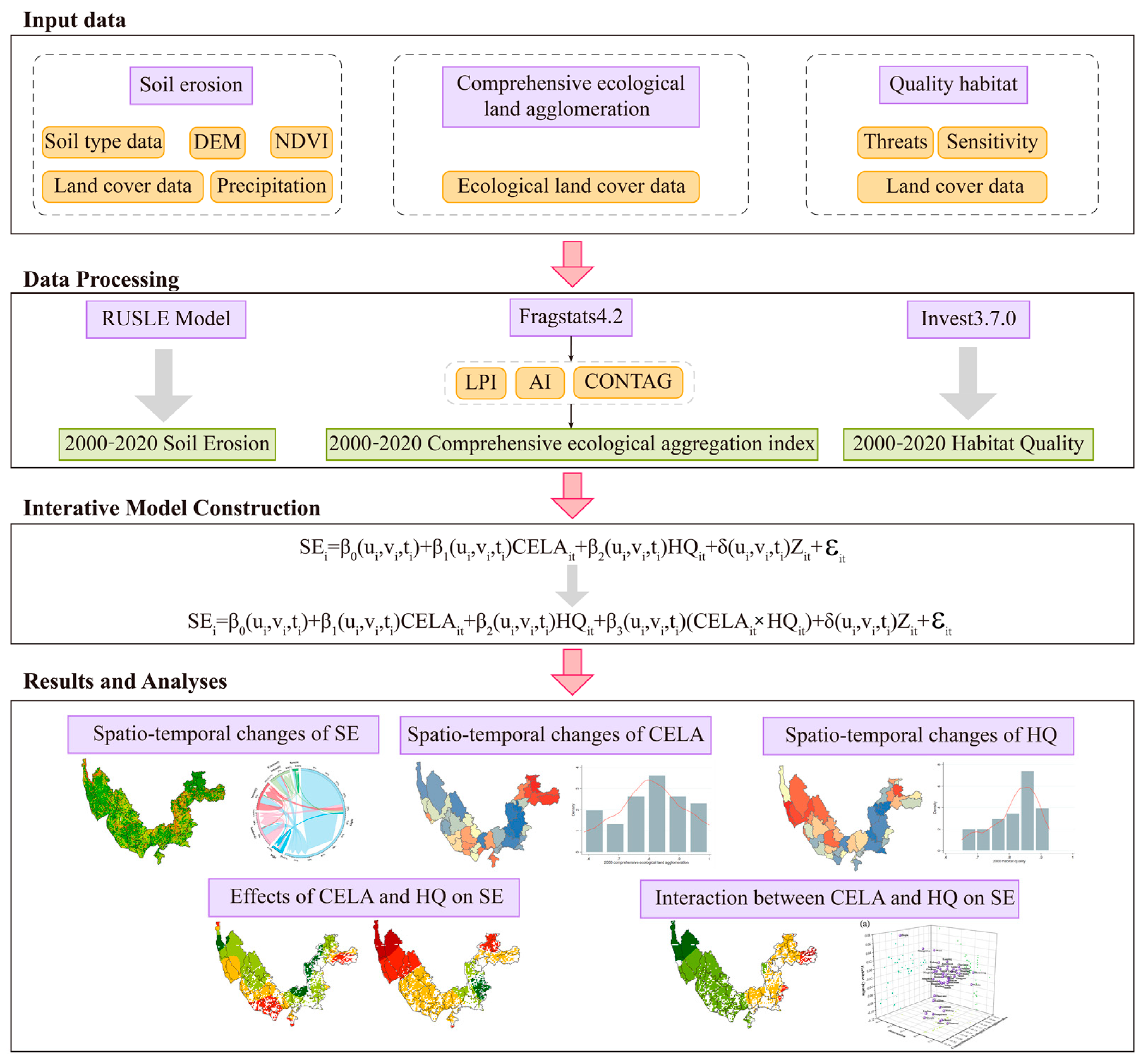
2. Research Design
3. Materials and Methods
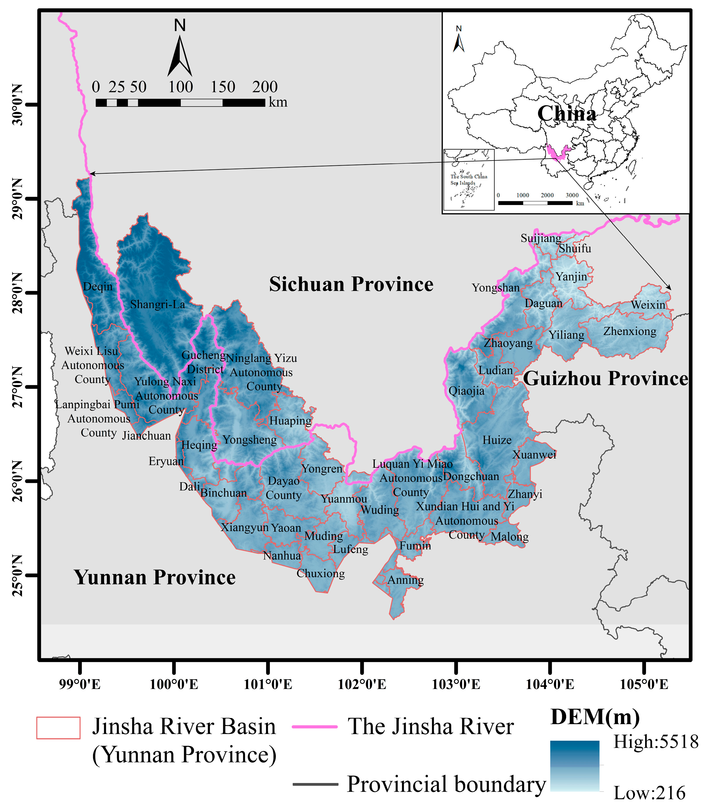
3.1. Study Area
3.2. Data Collection
3.3. Methods
3.3.1. RUSLE Model
3.3.2. Comprehensive Ecological Land Agglomeration
3.3.3. Habitat Quality Assessment Model
3.3.4. Spatial Autocorrelation Analysis
3.3.5. Geographic and Temporally Weighted Regression (GTWR)
4. Results
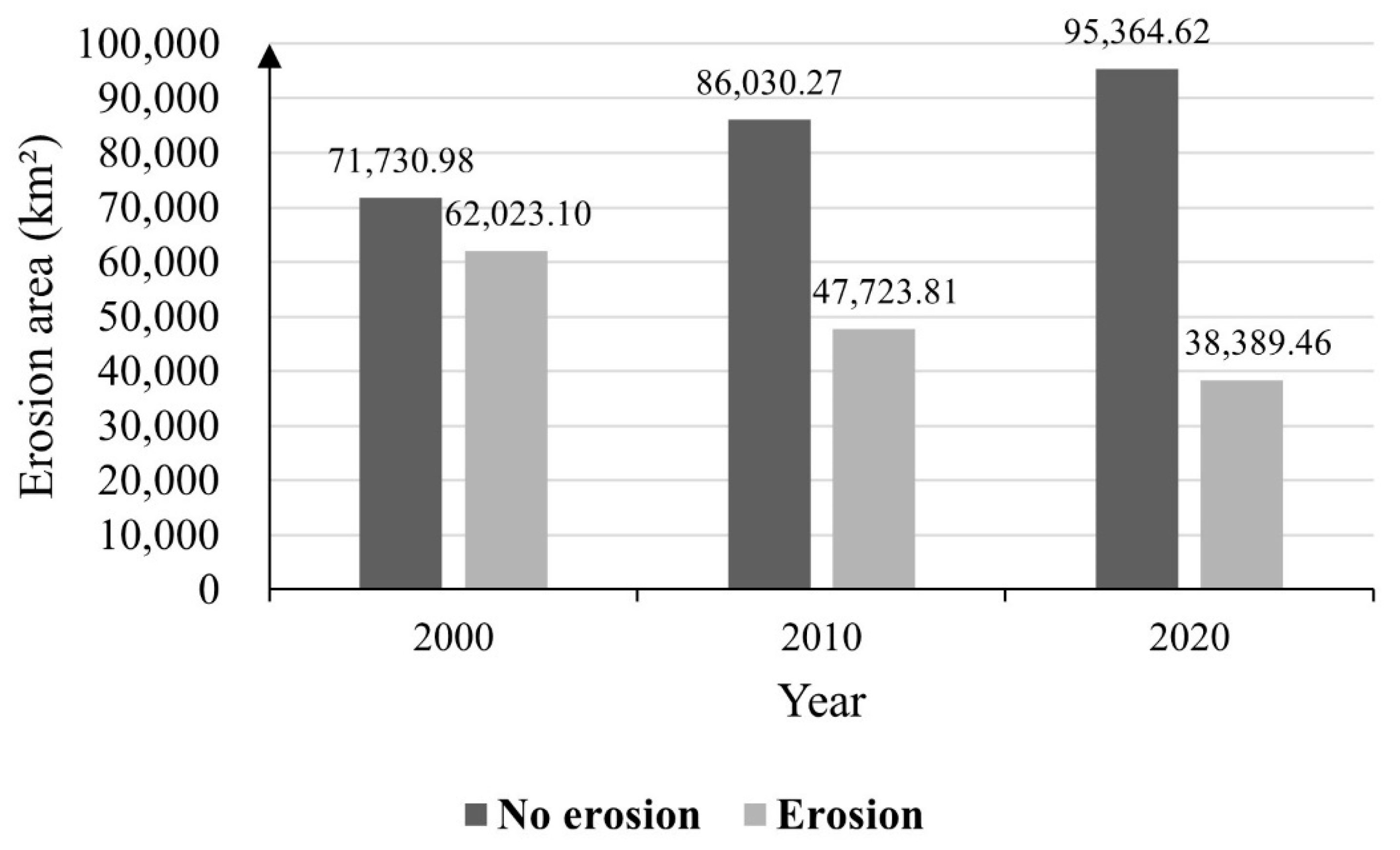
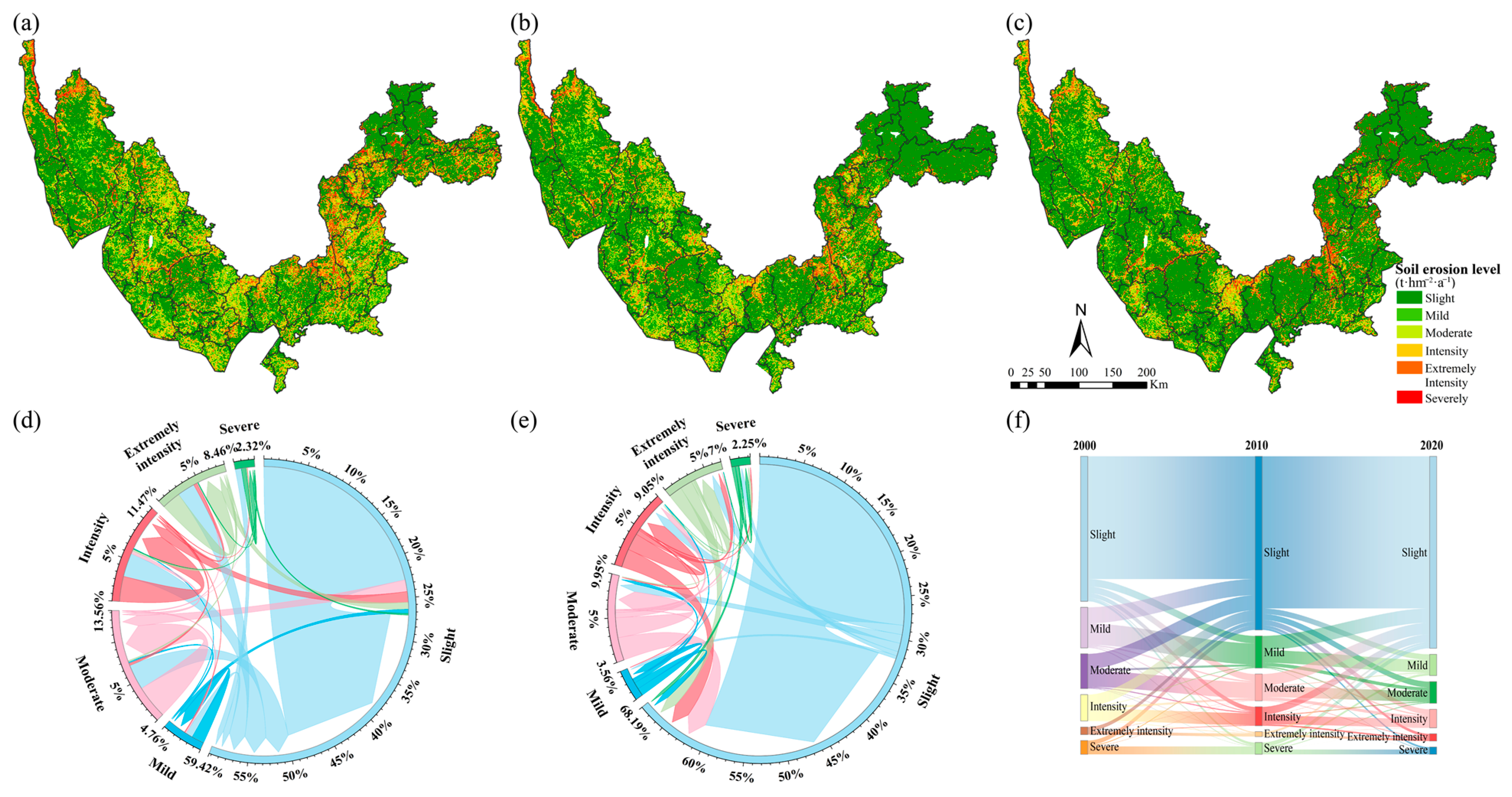
4.1. Spatio-Temporal Changes of Soil Erosion
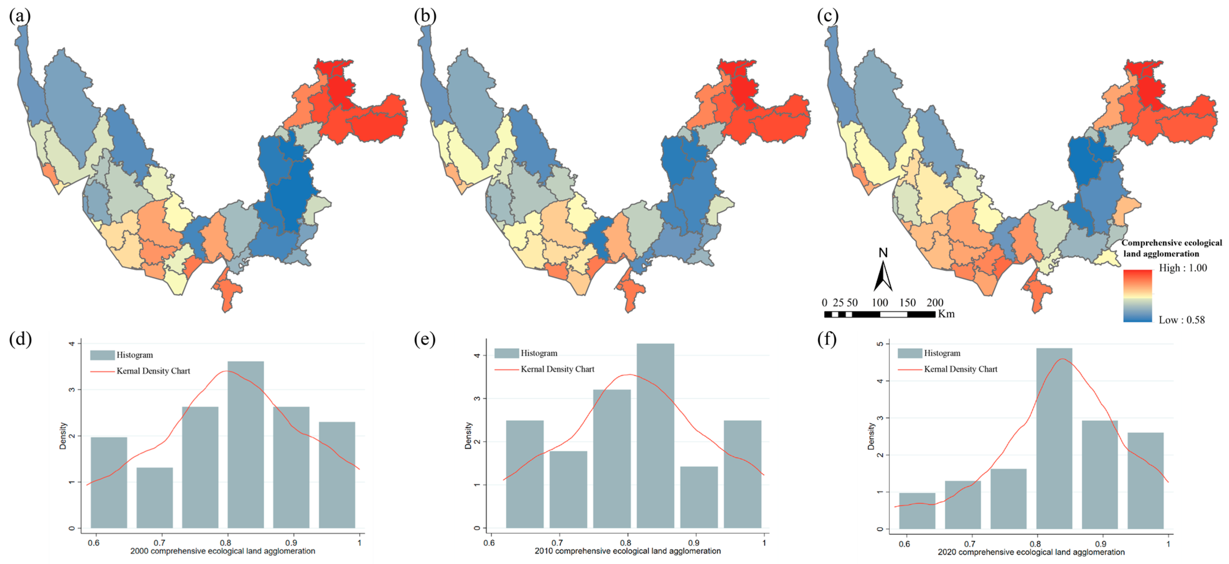
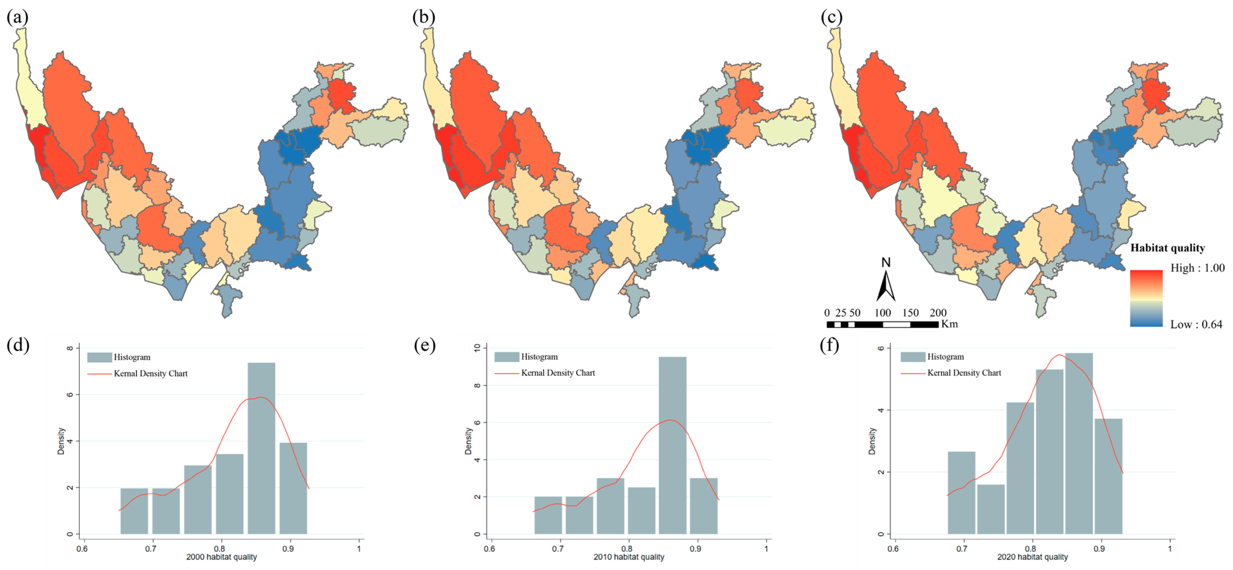
4.2. Spatio–Temporal Changes of the Comprehensive Ecological Land Agglomeration and Habitat Quality
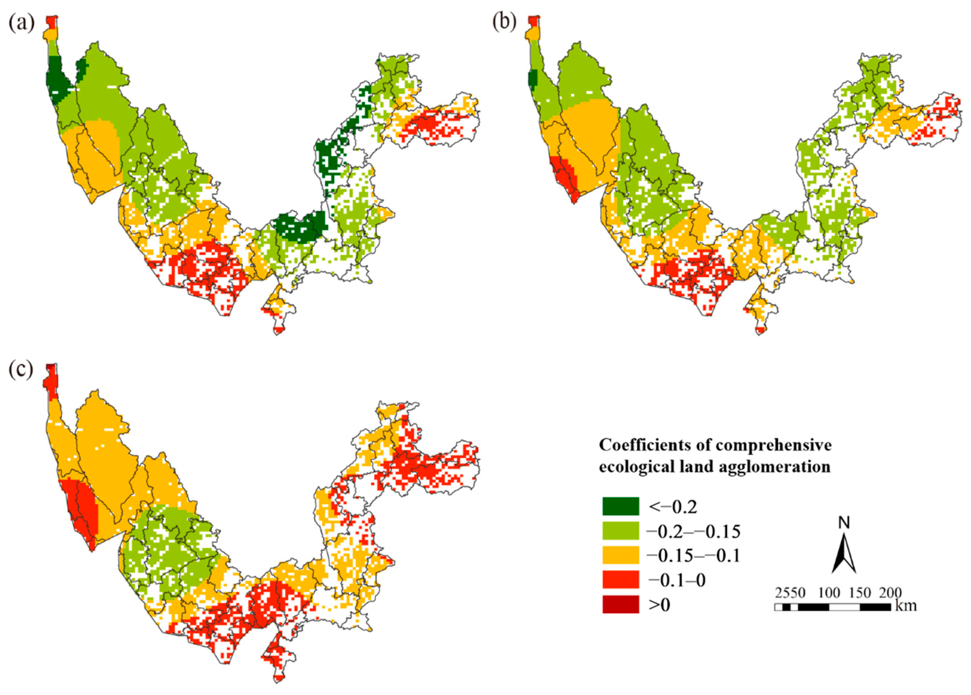
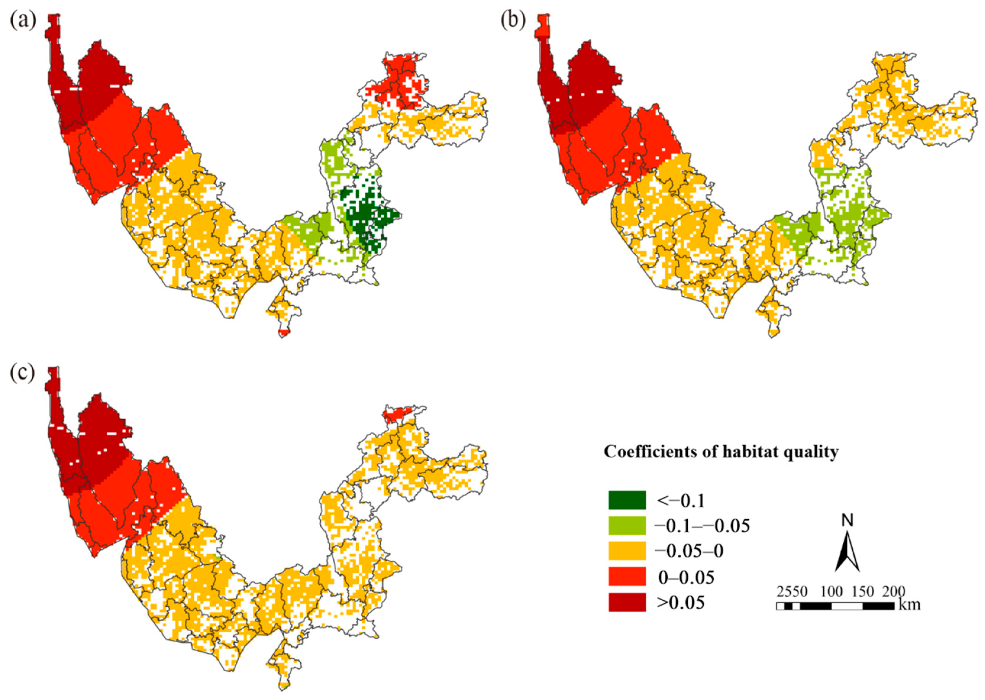
4.3. Effects of Comprehensive Ecological Land Agglomeration and Habitat Quality on Soil Erosion
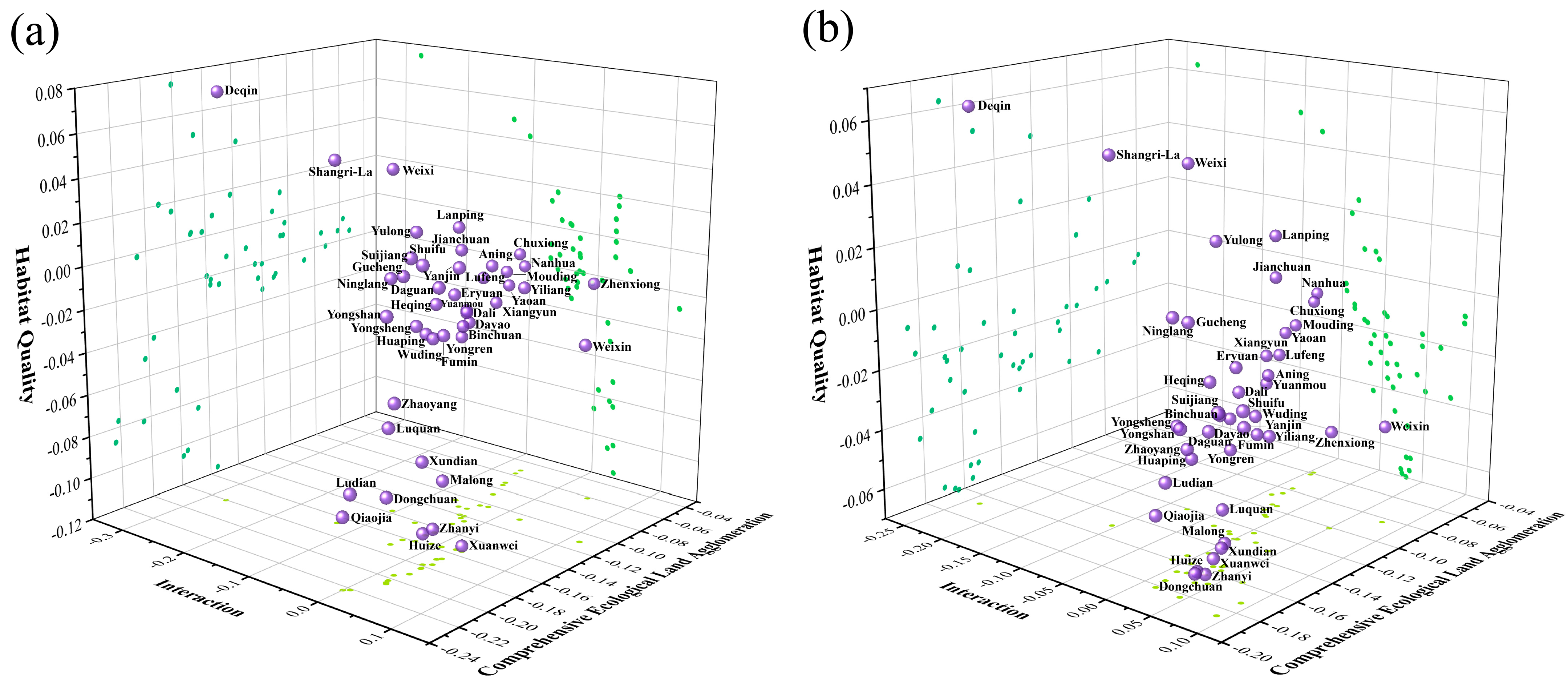
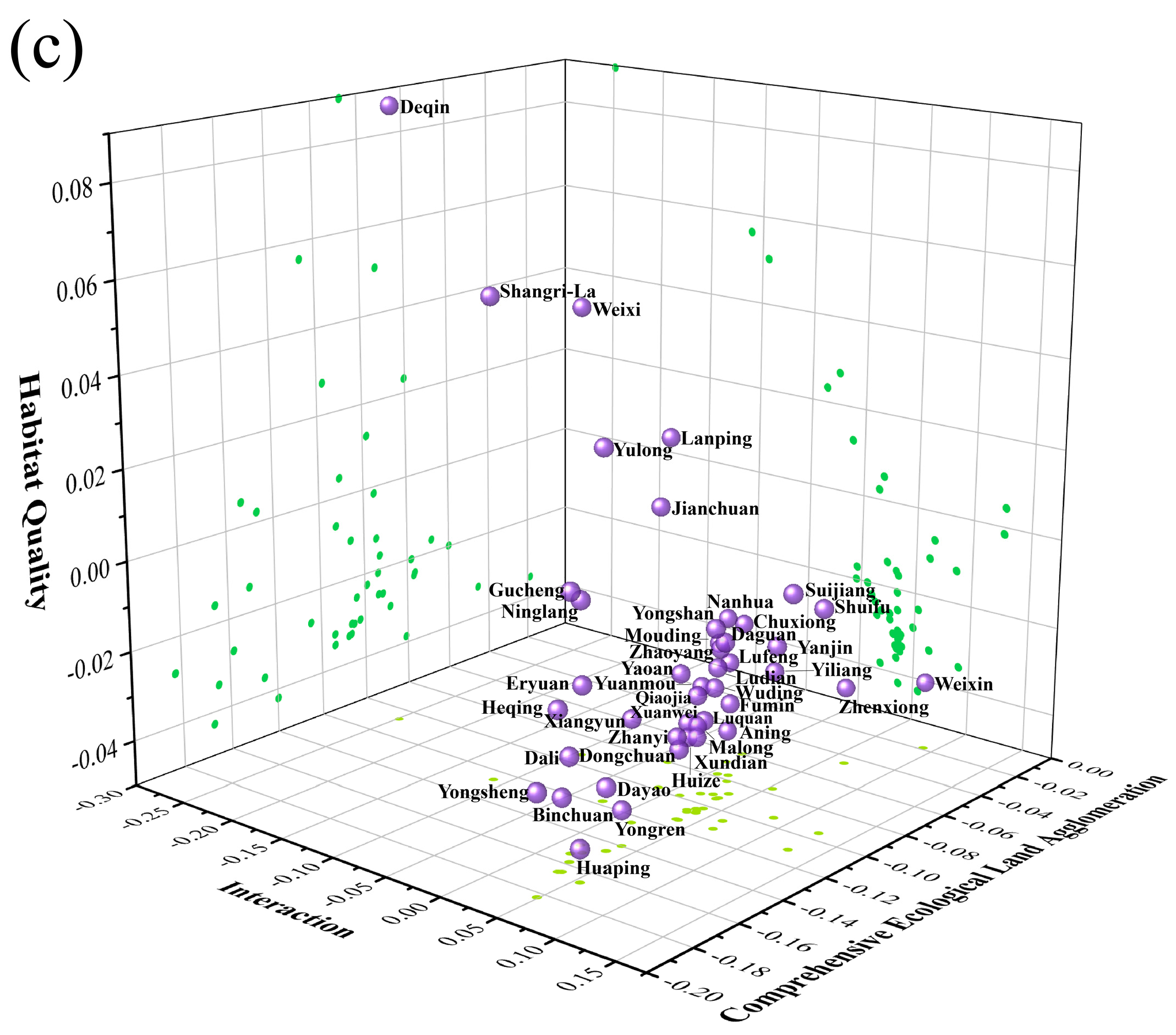
4.4. Interaction between Comprehensive Ecological Land Agglomeration and Habitat Quality on Soil Erosion
5. Discussion
5.1. Feasibility and Rationality of Methods
5.2. Interaction among Comprehensive Ecological Land Agglomeration, Habitat Quality, and Soil Erosion in the Jinsha River Catchment in Yunnan Province
5.3. The Management of Ecological Land Agglomeration and Restoration of Habitat Quality Are Effective Tools for Soil Erosion Management
5.4. Strategies for Ecological Land Agglomeration Management and Habitat Quality Restoration
6. Conclusions
Author Contributions
Funding
Data Availability Statement
Conflicts of Interest
References
- Li, Z.W.; Ning, K.; Chen, J.; Liu, C.; Wang, D.Y.; Nie, X.D.; Hu, X.Q.; Wang, L.X.; Wang, T.W. Soil and water conservation effects driven by the implementation of ecological restoration projects: Evidence from the red soil hilly region of China in the last three decades. J. Clean. Prod. 2020, 260, 121109. [Google Scholar] [CrossRef]
- Xu, F.J.; Zhao, W.J.; Yan, T.T.; Qin, W.; Chen, H.A. Can slope spectrum information entropy replace slope length and steepness factor: A case study of the rocky mountain area in northern China. Catena 2022, 212, 106047. [Google Scholar] [CrossRef]
- Li, Y.; Li, Y.R.; Fang, B.; Wang, Q.Y.; Chen, Z.F. Impacts of ecological programs on land use and ecosystem services since the 1980s: A case-study of a typical catchment on the Loess Plateau, China. Land Degrad. Dev. 2022, 33, 3271–3282. [Google Scholar] [CrossRef]
- van Zelm, R.; van der Velde, M.; Balkovic, J.; Cengic, M.; Elshout, P.M.F.; Koellner, T.; Núñez, M.; Obersteiner, M.; Schmid, E.; Huijbregts, M.A.J. Spatially explicit life cycle impact assessment for soil erosion from global crop production. Ecosyst. Serv. 2018, 30, 220–227. [Google Scholar] [CrossRef]
- Abdulkareem, J.H.; Pradhan, B.; Sulaiman, W.N.A.; Jamil, N.R. Prediction of spatial soil loss impacted by long-term land-use/land-cover change in a tropical watershed. Geosci. Front. 2019, 10, 389–403. [Google Scholar] [CrossRef]
- Ochoa, P.A.; Fries, A.; Mejía, D.; Burneo, J.I.; Ruíz-Sinoga, J.D.; Cerdà, A. Effects of climate, land cover and topography on soil erosion risk in a semiarid basin of the Andes. Catena 2016, 140, 31–42. [Google Scholar] [CrossRef]
- Wang, L.; Yan, H.; Wang, X.W.; Wang, Z.; Yu, S.X.; Wang, T.W.; Shi, Z.H. The potential for soil erosion control associated with socio-economic development in the hilly red soil region, southern China. Catena 2020, 194, 104678. [Google Scholar] [CrossRef]
- Pili, S.; Serra, P.; Salvati, L. Landscape and the city: Agro-forest systems, land fragmentation and the ecological network in Rome, Italy. Urban For. Urban Green. 2019, 41, 230–237. [Google Scholar] [CrossRef]
- Liu, Q.-Q.; Chen, L.; Li, J.-C. Influences of slope gradient on soil erosion. Appl. Math. Mech. 2001, 22, 510–519. [Google Scholar] [CrossRef]
- Shi, P.; Li, P.; Li, Z.; Sun, J.; Wang, D.; Min, Z. Effects of grass vegetation coverage and position on runoff and sediment yields on the slope of Loess Plateau, China. Agric. Water Manag. 2022, 259, 107231. [Google Scholar] [CrossRef]
- Yang, M.; Li, X.; Hu, Y.; He, X. Assessing effects of landscape pattern on sediment yield using sediment delivery distributed model and a landscape indicator. Ecol. Indic. 2012, 22, 38–52. [Google Scholar] [CrossRef]
- Zhao, G.; Gao, P.; Tian, P.; Sun, W.; Hu, J.; Mu, X. Assessing sediment connectivity and soil erosion by water in a representative catchment on the Loess Plateau, China. Catena 2020, 185, 104284. [Google Scholar] [CrossRef]
- Ferretti, V.; Pomarico, S. Ecological land suitability analysis through spatial indicators: An application of the Analytic Network Process technique and Ordered Weighted Average approach. Ecol. Indic. 2013, 34, 507–519. [Google Scholar] [CrossRef]
- Kemp, K.K. Environmental Modeling with GIS: A Strategy for Dealing with Spatial Continuity; University of California: Santa Barbara, CA, USA, 1992. [Google Scholar]
- Xia, N.; Hai, W.; Tang, M.; Song, J.; Quan, W.; Zhang, B.; Ma, Y. Spatiotemporal evolution law and driving mechanism of production–living–ecological space from 2000 to 2020 in Xinjiang, China. Ecol. Indic. 2023, 154, 110807. [Google Scholar] [CrossRef]
- Shi, M.; Wu, H.; Fan, X.; Jia, H.; Dong, T.; He, P.; Baqa, M.F.; Jiang, P. Trade-offs and synergies of multiple ecosystem services for different land use scenarios in the yili river valley, China. Sustainability 2021, 13, 1577. [Google Scholar] [CrossRef]
- Yohannes, H.; Soromessa, T.; Argaw, M.; Dewan, A. Spatio-temporal changes in habitat quality and linkage with landscape characteristics in the Beressa watershed, Blue Nile basin of Ethiopian highlands. J. Environ. Manag. 2021, 281, 111885. [Google Scholar] [CrossRef]
- Wei, J.; Hou, L.; He, X. An assessment of human versus climatic impacts on large-sized basin erosion: The case of the upper Yangtze River. Nat. Hazards 2014, 74, 405–420. [Google Scholar] [CrossRef]
- Li, J.; Zhou, Z.X. Coupled analysis on landscape pattern and hydrological processes in Yanhe watershed of China. Sci. Total Environ. 2015, 505, 927–938. [Google Scholar] [CrossRef]
- Liu, Y.; Zhang, C.; Zeng, H. Constraint effects among several key ecosystem service types and their influencing factors: A case study of the Pearl River Delta, China. Ecol. Indic. 2023, 146, 109883. [Google Scholar] [CrossRef]
- Guo, L.; Liu, R.; Men, C.; Wang, Q.; Miao, Y.; Shoaib, M.; Wang, Y.; Jiao, L.; Zhang, Y. Multiscale spatiotemporal characteristics of landscape patterns, hotspots, and influencing factors for soil erosion. Sci. Total Environ. 2021, 779, 146474. [Google Scholar] [CrossRef]
- Shen, G.; Chen, N.; Wang, W.; Chen, Z. WHU-SGCC: A novel approach for blending daily satellite (CHIRP) and precipitation observations over the Jinsha River basin. Earth Syst. Sci. Data 2019, 11, 1711–1744. [Google Scholar] [CrossRef]
- Liu, S.; Wang, D.; Miao, W.; Wang, Z.; Zhang, P.; Li, D. Characteristics of runoff and sediment load during flood events in the Upper Yangtze River, China. J. Hydrol. 2023, 620, 129433. [Google Scholar] [CrossRef]
- Zhu, Z.; Fu, Y.; Woodcock, C.E.; Olofsson, P.; Vogelmann, J.E.; Holden, C.; Wang, M.; Dai, S.; Yu, Y. Including land cover change in analysis of greenness trends using all available Landsat 5, 7, and 8 images: A case study from Guangzhou, China (2000–2014). Remote Sens. Environ. 2016, 185, 243–257. [Google Scholar] [CrossRef]
- Zhang, F.; Tiyip, T.; Feng, Z.D.; Kung, H.T.; Johnson, V.C.; Ding, J.L.; Tashpolat, N.; Sawut, M.; Gui, D.W. Spatio-Temporal Patterns of Land Use/Cover Changes Over the Past 20 Years in the Middle Reaches of the Tarim River, Xinjiang, China. Land Degrad. Dev. 2015, 26, 284–299. [Google Scholar] [CrossRef]
- Gao, J.; Wang, H. Temporal analysis on quantitative attribution of karst soil erosion: A case study of a peak-cluster depression basin in Southwest China. Catena 2019, 172, 369–377. [Google Scholar] [CrossRef]
- Yonaba, R.; Koïta, M.; Mounirou, L.A.; Tazen, F.; Queloz, P.; Biaou, A.C.; Niang, D.; Zouré, C.; Karambiri, H.; Yacouba, H. Spatial and transient modelling of land use/land cover (LULC) dynamics in a Sahelian landscape under semi-arid climate in northern Burkina Faso. Land Use Policy 2021, 103, 105305. [Google Scholar] [CrossRef]
- Aneseyee, A.B.; Elias, E.; Soromessa, T.; Feyisa, G.L. Land use/land cover change effect on soil erosion and sediment delivery in the Winike watershed, Omo Gibe Basin, Ethiopia. Sci. Total Environ. 2020, 728, 138776. [Google Scholar] [CrossRef]
- Fu, B.J.; Zhao, W.W.; Chen, L.D.; Zhang, Q.J.; Lü, Y.H.; Gulinck, H.; Poesen, J. Assessment of soil erosion at large watershed scale using RUSLE and GIS: A case study in the Loess Plateau of China. Land Degrad. Dev. 2005, 16, 73–85. [Google Scholar] [CrossRef]
- Arnoldus, H. Methodology used to determine the maximum potential average annual soil loss due to sheet and rill erosion in Morocco. Environ. Sci. 1977, 34, 39–51. Available online: http://www.oalib.com/references/9333552 (accessed on 6 September 2023).
- Williams, J.R.; Greenwood, D.J.; Nye, P.H.; Walker, A. The erosion-productivity impact calculator (EPIC) model: A case history. Philos. Trans. R. Soc. Lond. Ser. B Biol. Sci. 1997, 329, 421–428. [Google Scholar] [CrossRef]
- Zhang, J.; Wang, N.; Wang, Y.; Wang, L.; Hu, A.; Zhang, D.; Su, X.; Chen, J. Responses of soil erosion to land-use changes in the largest tableland of the Loess Plateau. Land Degrad. Dev. 2021, 32, 3598–3613. [Google Scholar] [CrossRef]
- Yu, Y.; Shen, Y.; Wang, J.; Wei, Y.; Liu, Z. Simulation and mapping of drought and soil erosion in Central Yunnan Province, China. Adv. Space Res. 2021, 68, 4556–4572. [Google Scholar] [CrossRef]
- Rao, W.; Shen, Z.; Duan, X. Spatiotemporal patterns and drivers of soil erosion in Yunnan, Southwest China: RULSE assessments for recent 30 years and future predictions based on CMIP6. Catena 2023, 220, 106703. [Google Scholar] [CrossRef]
- Guo, X.; Chang, Q.; Liu, X.; Bao, H.; Zhang, Y.; Tu, X.; Zhu, C.; Lv, C.; Zhang, Y. Multi-dimensional eco-land classification and management for implementing the ecological redline policy in China. Land Use Policy 2018, 74, 15–31. [Google Scholar] [CrossRef]
- Li, J.; Zhou, K.; Xie, B.; Xiao, J. Impact of landscape pattern change on water-related ecosystem services: Comprehensive analysis based on heterogeneity perspective. Ecol. Indic. 2021, 133, 108372. [Google Scholar] [CrossRef]
- Dale, V.H.; Polasky, S. Measures of the effects of agricultural practices on ecosystem services. Ecol Econ. 2007, 64, 286–296. [Google Scholar] [CrossRef]
- Sun, X.; Yu, Y.; Wang, J.; Liu, W. Analysis of the Spatiotemporal Variation in Habitat Quality Based on the InVEST Model- A Case Study of Shangri-La City, Northwest Yunnan, China. J. Phys. Conf. Ser. 2021, 1961, 012016. [Google Scholar] [CrossRef]
- Lei, J.; Chen, Y.; Li, L.; Chen, Z.; Chen, X.; Wu, T.; Li, Y. Spatiotemporal change of habitat quality in Hainan Island of China based on changes in land use. Ecol. Indic. 2022, 145, 109707. [Google Scholar] [CrossRef]
- Zhao, X.; Deng, C.; Huang, X.; Kwan, M.-P. Driving forces and the spatial patterns of industrial sulfur dioxide discharge in China. Sci. Total Environ. 2017, 577, 279–288. [Google Scholar] [CrossRef]
- Huang, B.; Wu, B.; Barry, M. Geographically and temporally weighted regression for modeling spatio-temporal variation in house prices. Int. J. Geogr. Inf. Sci. 2010, 24, 383–401. [Google Scholar] [CrossRef]
- Hu, J.; Zhang, J.; Li, Y. Exploring the spatial and temporal driving mechanisms of landscape patterns on habitat quality in a city undergoing rapid urbanization based on GTWR and MGWR: The case of Nanjing, China. Ecol. Indic. 2022, 143, 109333. [Google Scholar] [CrossRef]
- Li, Y.; Bai, X.; Zhou, Y.; Qin, L.; Tian, X.; Tian, Y.; Li, P. Spatial–Temporal Evolution of Soil Erosion in a Typical Mountainous Karst Basin in SW China, Based on GIS and RUSLE. Arab. J. Sci. Eng. 2016, 41, 209–221. [Google Scholar] [CrossRef]
- Ran, C.; Wang, S.; Bai, X.; Tan, Q.; Zhao, C.; Luo, X.; Chen, H.; Xi, H. Trade-offs and synergies of ecosystem services in southwestern China. Environ. Eng. Sci. 2020, 37, 669–678. [Google Scholar] [CrossRef]
- Sun, L.; Yu, H.; Sun, M.; Wang, Y. Coupled impacts of climate and land use changes on regional ecosystem services. J. Environ. Manag. 2023, 326, 116753. [Google Scholar] [CrossRef]
- Quinton, J.N.; Govers, G.; Van Oost, K.; Bardgett, R.D. The impact of agricultural soil erosion on biogeochemical cycling. Nat. Geosci. 2010, 3, 311–314. [Google Scholar] [CrossRef]
- Singh, G.; Panda, R.K. Grid-cell based assessment of soil erosion potential for identification of critical erosion prone areas using USLE, GIS and remote sensing: A case study in the Kapgari watershed, India. Int. Soil Water Conserv. Res. 2017, 5, 202–211. [Google Scholar] [CrossRef]
- Yan, Y.; Dai, Q.; Wang, X.; Jin, L.; Mei, L. Response of shallow karst fissure soil quality to secondary succession in a degraded karst area of southwestern China. Geoderma 2019, 348, 76–85. [Google Scholar] [CrossRef]
- Koulouri, M.; Giourga, C. Land abandonment and slope gradient as key factors of soil erosion in Mediterranean terraced lands. Catena 2007, 69, 274–281. [Google Scholar] [CrossRef]
- Li, P.; Zuo, D.; Xu, Z.; Zhang, R.; Han, Y.; Sun, W.; Pang, B.; Ban, C.; Kan, G.; Yang, H. Dynamic changes of land use/cover and landscape pattern in a typical alpine river basin of the Qinghai-Tibet Plateau, China. Land Degrad. Dev. 2021, 32, 4327–4339. [Google Scholar] [CrossRef]
- Li, W.; Zinda, J.A.; Zhang, Z. Does the “Returning Farmland to Forest Program” Drive Community-Level Changes in Landscape Patterns in China? Forests 2019, 10, 933. [Google Scholar] [CrossRef]
- Dong, J.; Guo, F.; Lin, M.; Zhang, H.; Zhu, P. Optimization of green infrastructure networks based on potential green roof integration in a high-density urban area—A case study of Beijing, China. Sci. Total Environ. 2022, 834, 155307. [Google Scholar] [CrossRef] [PubMed]
- Valeri, S.; Zavattero, L.; Capotorti, G. Ecological Connectivity in Agricultural Green Infrastructure: Suggested Criteria for Fine Scale Assessment and Planning. Land 2021, 10, 807. [Google Scholar] [CrossRef]
- Wang, F.; Yu, Q.; Qiu, S.; Xu, C.; Ma, J.; Liu, H. Study on the relationship between topological characteristics of ecological spatial network and soil conservation function in southeastern Tibet, China. Ecol. Indic. 2023, 146, 109791. [Google Scholar] [CrossRef]
- Wang, D.L.; Ding, W.L. Spatial pattern of the ecological environment in Yunnan Province. PLoS ONE 2021, 16, e0248090. [Google Scholar] [CrossRef]
- Zhang, Z.; Hu, Z.; Zhong, F.; Cheng, Q.; Wu, M. Spatio-Temporal Evolution and Influencing Factors of High Quality Development in the Yunnan–Guizhou, Region Based on the Perspective of a Beautiful China and SDGs. Land 2022, 11, 821. [Google Scholar] [CrossRef]


| Agglomeration Index | Min | Max | Mean | SD |
|---|---|---|---|---|
| LPI | 22.22 | 100 | 86.29 | 27.67 |
| AI | 0 | 100 | 86.98 | 28.62 |
| CONTAG | 0 | 55.30 | 17.65 | 36.36 |
| Threat | Max Distance | Weight | DECAY |
|---|---|---|---|
| Cropland | 6 | 0.7 | linear |
| Unused | 3 | 0.5 | linear |
| Impervious | 10 | 1 | exponential |
| Land Use Types | Habitat | Cropland | Unused | Impervious |
|---|---|---|---|---|
| Cropland | 0.5 | 0.5 | 0 | 0.4 |
| Forest | 1 | 1 | 0.6 | 0.5 |
| Shrub | 0.8 | 0.8 | 0.6 | 0.5 |
| Grassland | 0.6 | 0.6 | 0.5 | 0.6 |
| Water | 0.8 | 0.8 | 0.4 | 0.4 |
| Unused | 0.3 | 0.3 | 0.3 | 0 |
| Impervious | 0 | 0 | 0 | 0 |
| Level | Soil Erosion Modulus/(t·hm−2a−1) | 2000 Area (km2) | 2000 Proportion | 2010 Area (km2) | 2010 Proportion | 2020 Area (km2) |
|---|---|---|---|---|---|---|
| Slight | 0–10 | 72,349.67 | 54.09% | 86,609.38 | 64.75% | 95,797.02 |
| Mild | 10–25 | 6841.27 | 5.11% | 5896.34 | 4.41% | 3632.97 |
| Moderate | 25–50 | 20,249.68 | 15.14% | 16,016.36 | 11.97% | 10,597.78 |
| Intensity | 50–80 | 17,320.33 | 12.95% | 13,375.6 | 10.00% | 10,844.87 |
| Extremely intensity | 80–150 | 13,179.67 | 9.85% | 9457.9 | 7.07% | 9260.03 |
| Severe | >150 | 3813.47 | 2.85% | 2398.5 | 1.79% | 3621.39 |
| Total | - | 133,754.08 | 100.00% | 133,754.1 | 100.00% | 133,754.1 |
| Year | 2020 | |||||||
|---|---|---|---|---|---|---|---|---|
| 2000 | Level | Slight | Mild | Moderate | Intensity | Extremely Intensity | Severe | Total |
| Slight | 62,890.81 | 1064.60 | 2630.14 | 2659.10 | 2164.92 | 940.09 | 72,349.67 | |
| Mild | 3173.54 | 2153.34 | 1031.79 | 462.33 | 20.27 | 0.00 | 6841.27 | |
| Moderate | 11,273.42 | 368.70 | 5859.67 | 1816.49 | 887.01 | 44.40 | 20,249.68 | |
| Intensity | 9533.18 | 46.33 | 888.94 | 4724.60 | 1718.04 | 409.24 | 17,320.33 | |
| Extremely intensity | 6798.80 | 0.00 | 187.25 | 1140.85 | 4069.24 | 983.53 | 13,179.67 | |
| Severe | 2127.28 | 0.00 | 0.00 | 41.50 | 400.55 | 1244.13 | 3813.47 | |
| Total | 95,797.02 | 3632.97 | 10,597.78 | 10,844.87 | 9260.03 | 3621.39 | 133,754.08 | |
| Year | Moran’s | Z Score | p Score |
|---|---|---|---|
| 2000 | 0.52 | 67.94 | 0.00 |
| 2010 | 0.53 | 68.82 | 0.00 |
| 2020 | 0.51 | 66.33 | 0.00 |
| Models | R2 Adjusted | Sigma | AICc |
|---|---|---|---|
| GWR | 0.616 | 0.620 | 21,148.6 |
| GTWR | 0.625 | 0.612 | 20,945.6 |
| Variable | Average Value | Standard Deviation | Minimum Value | Maximum Values |
|---|---|---|---|---|
| intercept | 0.7906 | 0.4208 | −0.2335 | 3.3109 |
| Comprehensive ecological land agglomeration | −0.4026 | 0.0861 | −0.6850 | −0.0344 |
| Habitat quality | −0.9047 | 0.3456 | −2.9933 | −0.4106 |
| R2 | 0.370 | |||
| Variable | Mean | Standard Deviation | Minimum Value | Maximum Values |
|---|---|---|---|---|
| Intercept | 0.0283 | 0.1620 | −0.1491 | 0.5699 |
| comprehensive ecological land agglomeration | −0.1383 | 0.0381 | −0.2538 | 0.0246 |
| Habitat quality | −0.0021 | 0.0430 | −0.1190 | 0.1130 |
| NDVI | −0.7912 | 0.2935 | −1.6782 | −0.5024 |
| Precipitation | 0.0696 | 0.0822 | −0.1633 | 0.3154 |
| Population | 0.0466 | 0.0859 | −0.2211 | 0.3599 |
| R2 | 0.625 | |||
| Variable | Mean | Standard Deviation | Minimum Value | Maximum Values |
|---|---|---|---|---|
| Intercept | 0.0390 | 0.1552 | −0.1392 | 0.5660 |
| Comprehensive ecological land agglomeration | −0.1337 | 0.0369 | −0.2573 | −0.0063 |
| Habitat quality | −0.0321 | 0.0478 | −0.4705 | 0.0261 |
| Interaction term | −0.0299 | 0.0886 | −0.5966 | 0.1677 |
| NDVI | −0.7958 | 0.2936 | −1.6856 | −0.5021 |
| Precipitation | 0.0696 | 0.0831 | −0.1630 | 0.3179 |
| Population | 0.0476 | 0.0851 | −0.1452 | 0.3594 |
| R2 | 0.639 | |||
Disclaimer/Publisher’s Note: The statements, opinions and data contained in all publications are solely those of the individual author(s) and contributor(s) and not of MDPI and/or the editor(s). MDPI and/or the editor(s) disclaim responsibility for any injury to people or property resulting from any ideas, methods, instructions or products referred to in the content. |
© 2024 by the authors. Licensee MDPI, Basel, Switzerland. This article is an open access article distributed under the terms and conditions of the Creative Commons Attribution (CC BY) license (https://creativecommons.org/licenses/by/4.0/).
Share and Cite
Wen, B.; Liu, C.; Tian, X.; Zhang, Q.; Huang, S.; Zhang, Y. Interactive Effects of Ecological Land Agglomeration and Habitat Quality on Soil Erosion in the Jinsha River Basin, China. Land 2024, 13, 229. https://doi.org/10.3390/land13020229
Wen B, Liu C, Tian X, Zhang Q, Huang S, Zhang Y. Interactive Effects of Ecological Land Agglomeration and Habitat Quality on Soil Erosion in the Jinsha River Basin, China. Land. 2024; 13(2):229. https://doi.org/10.3390/land13020229
Chicago/Turabian StyleWen, Bo, Chenxi Liu, Xu Tian, Qi Zhang, Shaolie Huang, and Yanyuan Zhang. 2024. "Interactive Effects of Ecological Land Agglomeration and Habitat Quality on Soil Erosion in the Jinsha River Basin, China" Land 13, no. 2: 229. https://doi.org/10.3390/land13020229
APA StyleWen, B., Liu, C., Tian, X., Zhang, Q., Huang, S., & Zhang, Y. (2024). Interactive Effects of Ecological Land Agglomeration and Habitat Quality on Soil Erosion in the Jinsha River Basin, China. Land, 13(2), 229. https://doi.org/10.3390/land13020229