Integrating Spatiotemporal and Travel-Related Information for Accurate Urban Passenger Profiling Using GANs

Abstract

The elaborate description of passenger travel profiles is of significant importance in urban planning, socioeconomic structural design, and individual travel preference analysis. Traditional models often lack consideration of personalized features and exhibit suboptimal performance in constructing spatiotemporal dependencies. To address these issues, this paper proposes a method that integrates spatiotemporal information with travel-related information and employs generative adversarial networks (GANs) for adversarial training. This method accurately fits the true distribution of user travel data, thereby providing detailed profiles of public transportation passengers’ travel behavior. Specifically, the proposed approach considers the complete travel chain of individuals, establishes a spatiotemporal constraint representation model, and utilizes GANs to simulate the distribution of passenger travel, obtaining more compact and high-level travel vector features. The empirical results demonstrate that the proposed method accurately captures passengers’ travel patterns in both the temporal and spatial dimensions, offering technical support for urban transportation planning.

1. Introduction

Modeling and representing human activities are crucial for understanding human activity patterns in urban sociospatial planning and individual travel preference analysis [1,2,3], which examines how social behaviors interact with spatial configurations in urban environments. This understanding is essential for optimizing public transportation systems and analyzing travel preferences at an individual level [4,5]. However, human travel activities are characterized by strong spatiotemporal correlations and are a collection of individual travel patterns [6,7]. Therefore, effectively integrating spatiotemporal and travel-related information is key to accurately characterizing and representing travel activity patterns [8].

Human travel activities exhibit certain group similarities, and early studies on human activity models were based on statistical approaches from a group perspective [9]. Classic models can be traced back to the gravity model from the last century [10], which defines human activity between cities as follows: the intensity of population migration is proportional to the product of the populations of the two cities and inversely proportional to the distance between them. Another classic model is the radiation model [11], which comprehensively considers factors such as job opportunities, income distribution, working conditions, population, and local random processes. This model fits actual data well and effectively simulates population flow and human activity migration between regions. Traditional models, represented by the gravity and radiation models, emphasize exploring human travel patterns, aiming to construct a general model to simulate human travel patterns. However, these models are relatively simple, consider only a single set of influencing factors, and are modeled from a group perspective, lacking consideration of individualized travel behavior characteristics [12].

Public transportation systems such as subways, buses, and ferries support a vast amount of daily population movement within cities, including the regular activities of commuters and residents as well as numerous random activities. These systems generate massive amounts of smart card data (SCD) daily, reaching terabytes or even larger scales [13]. SCD serve as an excellent medium to describe public travel activities, providing a new opportunity to study travel patterns and preferences from a different perspective.

From a data-driven perspective, modeling human travel activities often focuses on individual travel patterns. Common modeling methods include Recurrent Neural Networks (RNNs) and Word2Vec [14]. These models can capture the temporal associations of individual travel and handle variable-length input and output sequences [15,16], achieving good results in practical applications. However, research on directly applying RNNs and similar network models to travel activity modeling tends to focus excessively on large-sample data-driven models while providing rough spatiotemporal feature modeling [17,18,19]. This approach often pays too much attention to single-trajectory information and neglects the complete travel chain information of individuals, thereby losing many personalized travel characteristics.

While much of the existing research on urban transportation planning focuses on aggregate travel behavior and general system-level optimization, there is a significant gap in the literature regarding personalized travel recommendations for individual passengers. Traditional models primarily rely on spatiotemporal data (e.g., location, time) to predict travel behavior, but they often overlook semantic information such as trip purpose and individual preferences, which are crucial for creating personalized travel profiles. This study aims to fill this gap by proposing a novel methodology that integrates both spatiotemporal and semantic data using generative adversarial networks (GANs), enabling the generation of more accurate, individualized travel recommendations and profiles for urban commuters.

Travel data encapsulate passenger preferences and activity behavior characteristics, serving as a fundamental data source for passenger travel profiling [20,21]. Based on passenger travel data, the goal of this study is to establish a refined expression model for human activity travel profiles. This paper proposes a method for expressing individual human travel activities by combining spatiotemporal information with travel-related information. It utilizes classical algorithms to characterize individual travel patterns and inputs the extracted activity patterns into generative adversarial networks (GANs) for adversarial training to fit the true distribution of the user’s travel data, thus representing the user’s travel activities. The model is data-driven and emphasizes the spatiotemporal characteristics of travel. The extracted travel profiles provide valuable insights into understanding user habits, behavior patterns, and personalized travel recommendations, and individual passengers can use them to improve the efficiency and comfort of their daily commutes. By analyzing their historical travel patterns and preferences, the model can provide tailored suggestions, such as optimal travel times or recommended routes to avoid congestion. The main contributions of this paper include the following:

(1) From a data-driven perspective, modeling individual travel by considering complete travel chain information.

(2) Considering the characteristics of public transportation, incorporating spatiotemporal constraints, and adding common travel features to the personalized travel representation. This system can offer tailored recommendations that optimize the travel experience for individual passengers, enhancing travel convenience and helping to alleviate congestion during peak periods.

(3) Using GANs’ adversarial training approach to simulate passenger travel distributions and obtaining more compact and high-level travel vector features specific to individual passengers and their unique spatiotemporal characteristics.

2. Related Work

2.1. Travel Activity Representation

The modeling and representation of human travel activities play a crucial role in understanding migration patterns between cities, urban socioeconomic structure planning, and individual travel preferences [2,3]. Understanding human travel behavior is key to analyzing personal activity patterns and optimizing urban functional zoning [4]. Human travel activities exhibit strong spatiotemporal correlations and are a collective representation of individual travel patterns [8]. Thus, effectively integrating spatiotemporal and travel-related information is crucial for accurately capturing and representing travel activity patterns.

Traditional research on human activity modeling often starts from a statistical perspective, focusing on group-level behaviors. Early models, such as the gravity model [10], defined inter-city human activity as proportional to the product of the populations of the two cities and inversely proportional to the distance between them. Another classical model, the radiation model [11], incorporates factors such as local work opportunities, income distribution, job conditions, and population, resulting in a high degree of fit with real-world data and accurately simulating migration and human activity flow. These traditional models, represented by the gravity and radiation models, primarily explore travel patterns from a group perspective and often lack consideration of personalized individual travel behaviors [12].

Recent advancements in computational resources and the rapid growth of trajectory data have led to the rise of deep learning techniques for travel activity modeling. Gong et al. [18] employed an agent-based modeling model for intra-urban activity simulation to explore user activity patterns. Mor et al. [18,19] used machine learning to cluster international urban tourists. Zhou et al. [22] utilized Variational Autoencoders (VAEs) for solving the user–trajectory matching problem. Chao et al. [23] proposed using autoencoders (AEs) to establish representations of individual trips and infer user travel purposes based on these representations. While these deep learning-based studies provide valuable insights and advancements, they often fall short in modeling spatiotemporal features, an area that this paper aims to address.

2.2. Generative Adversarial Networks

Generative adversarial networks (GANs) are powerful deep learning models that play a significant role in solving complex data distribution fitting problems. Introduced by I.J. Goodfellow in 2014 [24], GANs have sparked significant research interest. This model is based on a “two-player zero-sum game”, where the network consists of a generator (G) and a discriminator (D). The generator aims to model the complex data distribution, while the discriminator’s goal is to distinguish between real and generated samples. The training process involves an adversarial game where G seeks to produce samples that are indistinguishable from real data, while D aims to accurately classify the samples as real or fake.

GANs offer a novel approach to representation learning through their adversarial game framework. Dai et al. [17] noted that previous graph representation models lacked constraints, reducing the robustness of representation results. They designed an Adversarial Network Embedding (ANE) model to enhance graph representation results by capturing the original graph structure using GANs. Wang et al. [25] proposed a Graph Generative Adversarial Net (GraphGAN) model, where the generator approximates the real distribution of neighboring nodes given a graph node, and the discriminator assesses the authenticity of samples generated by the generator. Zhou et al. [26] applied adversarial game principles to solve Point of Interest (POI) recommendation problems, using a recommender to learn the latent real distribution of POIs and a discriminator to evaluate the authenticity of generated and real samples. Gao et al. [27] proposed a semi-supervised learning model for user trajectory matching (Trajectory User Linking, TUL), employing adversarial networks to regularize the data distribution of user trajectories. GANs have demonstrated unique advantages in the process of human travel modeling, providing a powerful tool for improving the methods proposed in this paper.

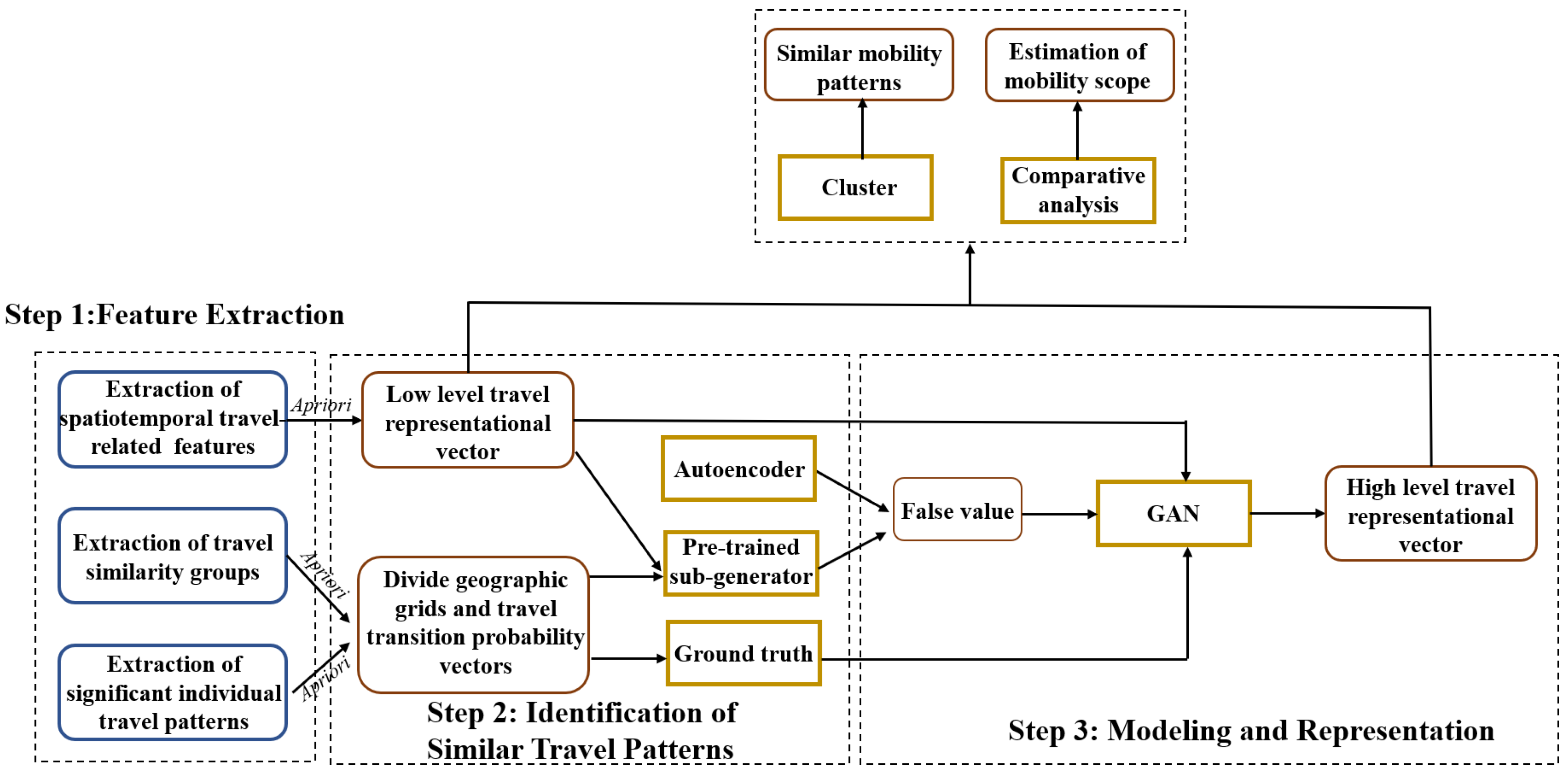
3. Materials and Methods

In this section, we present the methodology used to construct detailed travel profiles of passengers by integrating spatiotemporal and travel-related information. The main goal of this section is to describe the process through which we combine travel data with travel-related features to accurately represent individual travel behaviors. This includes the extraction of key travel characteristics, the application of an improved Apriori algorithm to identify significant travel patterns, and the use of generative adversarial networks (GANs) for adversarial training to generate high-level representations of travel data.

3.1. Definitions

Specifically, we use an improved Apriori algorithm to extract significant individual travel patterns and identify similar individuals, which are then utilized for generating adversarial vector representations of travel activities. The research objective of this study can be expressed as follows:

$$y=f(x_1,x_2,\dots ,x_t)$$

(1)

where $x_1,x_2,\dots ,x_t$ are the time-series data of passenger travel, $f(·)$ is the proposed algorithm, and y represents the detailed travel profile of a passenger, which includes various features such as the passenger’s travel time patterns, spatial movement (origins and destinations), and travel-related characteristics (trip duration, number of transfers, and travel purpose). These features are the target output of the model, which aims to learn and predict the full travel behavior of an individual passenger. To create a comprehensive passenger profile, it is essential to consider travel time features, spatial features, and travel-related features, defined as follows:

Travel time features: The features extracted from the travel chain include the trip’s start time, To, and end time, Td. The raw time data, recorded in formats such as “18:34:31”, cannot be directly used in their DateTime format for model training due to computational limitations and the need to reflect the periodic nature of time. Specifically, the times “23:59:11” and “00:01:01” are similar and should not be treated as separate. To capture the periodicity of time features, this study projects the actual time features onto a two-dimensional circular plane [28]. Each time feature is represented by a point coordinate ($o_x$, $o_y$) on the circle, as Equations (2)–(4).

(i) DateTime-format time features are converted into hours as the basic unit of measurement, as shown in Equation (2).

$$FTime=DTime\left(h\right)+{\displaystyle \frac{DTime\left(m\right)}{60}}+{\displaystyle \frac{DTime\left(s\right)}{3600}}$$

(2)

(ii) Circular projection conversion is performed using Equations (3) and (4), where T represents the period, i.e., 24 h.

$$o_x=cos\left({\displaystyle \frac{2\pi \ast FTime}{T}}\right)$$

(3)

$$o_y=sin\left({\displaystyle \frac{2\pi \ast FTime}{T}}\right)$$

(4)

Both the start and end times are converted, expanding from 2 feature dimensions to 4 feature dimensions.

Travel spatial features: To improve computational accuracy, the original coordinates in the WGS84 coordinate system are projected into the Universal Mercator projection, and all subsequent calculations use this projected coordinate system. ($x_{um},y_{um}$) = trans($x_{wg84},y_{wg84}$), where trans represents the coordinate conversion function, and this article uses the pyproj library for conversion. This results in 4 feature dimensions for both the starting and ending coordinates.

Travel-related features: Travel-related features are crucial components of trip information. Three travel-related features are extracted for travel-related information representation: trip duration, number of stations passed, and transfer counts. Trip duration and the number of stations passed represent the time and travel spatial sequences of the passenger’s trip, respectively, while transfer counts indicate the intensity of the passenger’s transfer behavior.

Travel Transition Probability Matrix: A two-dimensional matrix, M, with dimensions for passenger travel activity statistics is established. Each element, m (i, j), of the M matrix represents the number of trips taken by passengers from the i-th urban grid to the j-th urban grid. From this, it can be seen that the i-th row of the M matrix represents all the trips taken by the passenger from the i-th urban grid, while the j-th column represents all the trips taken by the passenger to the j-th urban grid. Specifically, for each row unit, the probability of traveling from that row to other places is calculated. For the j-th element in the i-th row, $\mathrm{m}\prime (\mathrm{i},\mathrm{j})={\displaystyle \frac{\mathrm{m}(\mathrm{i},\mathrm{j})}{\sum _j\mathrm{m}(\mathrm{i},\mathrm{j})}}$, taking the maximum probability as the representation of the row, i.e., $\mathrm{m}{\mathrm{m}}_{\mathrm{i}}\prime$ = max (${\mathrm{m}}^{\prime }$(i, 1),..., ${\mathrm{m}}^{\prime }$(i, n)), where n represents the number of geographic grids. So, we obtain a vector of length n representing the departure characteristics of the passenger, and the same applies to the columns.

Travel chain information: this can be represented as ${chain}_i=\left\{c_{i,1},c_{i,2},\dots ,c_{i,n}\right\},$ which represents the stations that the i-th passenger passes through from $c_{i,1}$ to $c_{i,n}$.

OD trip: this means the origin and destination, namely ${\mathrm{O}}_i$ = {$O_{i,x},O_{i,y}$},${\mathrm{D}}_i$={$D_{i,x},D_{i,y}$}, where $O_{i,x},O_{i,y}$,$D_{i,x},{and D}_{i,y}$ represent the coordinates of the origin and destination points, respectively. Each trip can thus be represented by a total of 11 feature dimensions. To accelerate model convergence and ensure that data have the same distribution scale, standardization (normalization) is applied to each feature column. This involves transforming the data to conform to a standard normal distribution with a mean of 0 and a variance of 1.

3.2. Algorithm Details

Figure 1 provides an overview of the methodology, illustrating how raw travel data flow through the system. The process begins with feature extraction (Step 1), where the raw data are processed to extract key travel features such as trip duration, number of stations passed, and number of transfers. These features are critical for understanding passenger behavior and are used to construct travel profiles.

Next, the identification of similar travel patterns (Step 2) is performed using an improved Apriori algorithm. This step identifies similar travel behaviors among passengers based on the extracted features, enabling the construction of a Travel Transition Probability Matrix that models the likelihood of transitions between travel states (such as location or time).

Finally, the modeling and representation stage (Step 3) uses generative adversarial networks (GANs) to create high-level representations of passenger travel activities. The GANs are trained to capture the distribution of travel data, generating more compact and high-level travel vector features that can be used for further analysis, prediction, or personalized recommendations.

3.3. Extraction of Significant Travel Patterns

Based on passenger travel activity data, this study focuses on representing individual travel behavior by extracting the OD (origin–destination) sequence set that best reflects the travel patterns of the passengers. Significant travel patterns for individuals should exhibit the following characteristics: (1) frequent travel characteristics: patterns that occur frequently in the travel data; (2) co-occurrence characteristics: activities that commonly occur together, indicating a symbiotic relationship; and (3) spatiotemporal constraints: travel interactions that must satisfy specific time thresholds and spatial limitations.

An association analysis algorithm provides a robust approach to addressing the above criteria. The traditional Apriori algorithm is commonly used to discover frequent itemsets in transaction data but suffers from inefficiencies when dealing with large datasets or complex constraints. Our improved version of the Apriori algorithm incorporates spatiotemporal constraints that are critical for the accurate classification of travel patterns in urban environments. For example, we introduce a time window constraint that limits frequent itemsets to those that occur within a specific timeframe (e.g., peak hours). Additionally, a spatial proximity constraint ensures that only those itemsets that represent travel patterns within the same region are considered, thus focusing on local travel patterns. This study uses the Apriori algorithm [29] by integrating spatiotemporal constraints into the calculations of support and confidence between data items, making it more applicable to real-world scenarios.

Specifically, if a passenger i has m trips within a defined research period, the travel chain can be represented as shown in Equation (5), where $P_i$ denotes locations and $d_i$ represents the time intervals between adjacent locations.

$$i_{trip}=\{P_1\stackrel{d_1}{\to }{P}_2\stackrel{d_2}{\to }{P}_3\to \dots \to P_{2m-1}\stackrel{d_{2m-1}}{\to }{P}_{2m}\}$$

(5)

For a travel chain of length m, the trips are arranged in ascending order based on their starting times, and the travel time between each trip, such as d₁ or d₂, is calculated as shown in Equation (5). This approach integrates the O (origin) and D (destination) of each trip in the travel chain to represent the passenger’s travel activity trajectory within the specified time interval, for example, $P_1\stackrel{d_1}{\to }{P}_2$ belong to ${trip}_1$, $P_{2m-1}\stackrel{d_{2m-1}}{\to }{P}_{2m}$ belong to ${trip}_m$.

Specifically, a set Q is defined to store the quadruple tuples (O, D, startDur, aveDur), representing the average travel time, aveDur, from the origin O to the destination D starting at time startDur. The inclusion of the departure time constraint accounts for significant fluctuations in travel times due to peak hours on weekdays. The startDur variable is predefined, dividing the 24 h day into intervals.

The entire database is then traversed to generate the candidate set R₁ and construct the Q set. Using a predefined support threshold, the frequent set L₁ is derived from the candidate set R₁. The process is then extended to find longer frequent pattern sets. If the frequent set L_k (where k represents the length of the frequent pattern data items in the set) meets the minimum length constraint, the itemsets satisfying the confidence constraint and spatiotemporal constraints are used to form the candidate set R^k+1. Members of R^k+1 that meet the support threshold form the frequent set L^k+1.

Meeting spatiotemporal constraints means that for an OD pair to be considered frequent and similar, it must satisfy the origin O, destination D, departure time interval startDur, and travel time constraints within the range of [aveDur∗(1−σ), aveDur∗(1+σ)]. This indicates the presence of frequent and symbiotic relationships. The frequent itemsets, L_Pattern, collectively form the total frequent set L, as shown in Algorithm 1.

Algorithm 1. Individual Significance Extraction Algorithm

Input: Collection of travel chains for all passengers within M days Trips = {T1, T2, T3, …, Tn-1, Tn},travel time fluctuation threshold σ, support threshold θ, confidence threshold δ, Minimum frequent pattern set length threshold γ. Output: Significant travel chain collection of all passengers within M days ETrips = {ET1, ET2, ET3, …, ETn-1, ETn} 1: Initialize Q←∅, L←∅, k←1, j←1 2: for each trip in Trips do 3:      R_j.append(trip.places) 4:      Q←UpdateQ(trip) 5: end for 6: Lj←ExtractFrequentPattern(Rj, θ) 7: while len(Lk) > γ do 8:      L.append(Lk) 9:      k←k + 1 10:    Rk←ExpandRSet(Lj, Lk, δ, Q, σ) 11:    Lk←ExtractFrequentPattern(Rk, θ) 12: End while 13: ETrips = ExtractPersonMotif(L, Trips)

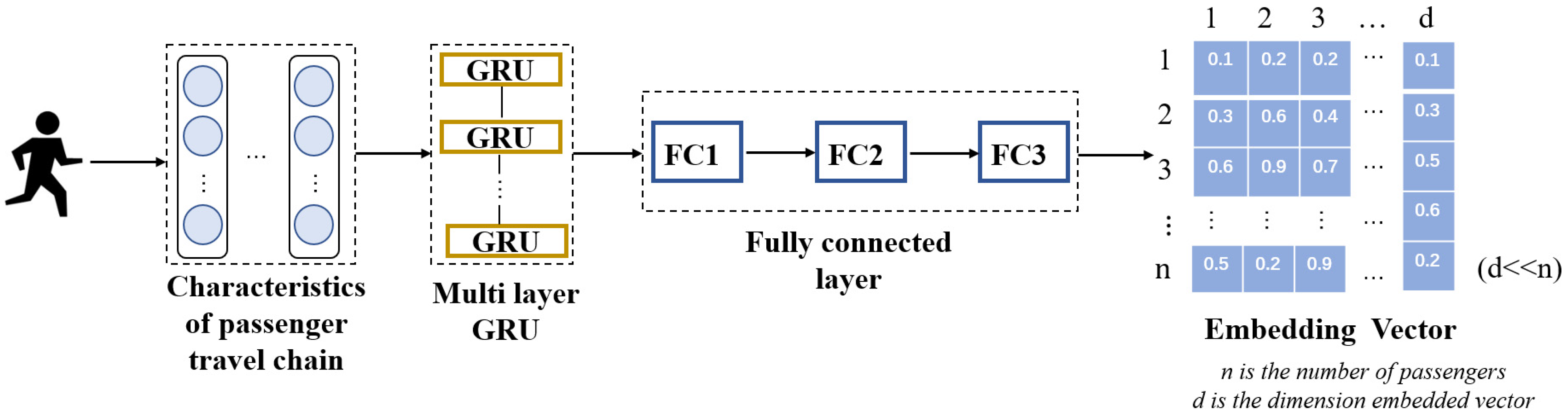
3.4. Travel Activity Vector Representation

Given the variable length of the results from Section 3.3 and the sparsity of bus trajectory data, directly applying these results to the model can be challenging. Therefore, this paper proposes a method for representing travel activity patterns based on geographical grids. The travel activity’s origin (O) and destination (D) information are transformed into passenger flows between corresponding geographical grids, termed travel activity transfers. By statistically calculating the frequency of these transfers, transfer probabilities are computed. These probabilities are then combined into a transfer probability vector, serving as the vector representation of passenger travel activities.

This study uses regional visit heat as the basis for geographical grid division. The grid division should adhere to a maximum heat limit. If an area’s heat is too high and meets the minimum regional size limit, it should be recursively divided into four smaller regions until each region’s flow heat does not exceed the maximum flow limit and the regional boundaries are not smaller than the minimum boundary limit. The specific implementation process is shown in Algorithm 2.

Algorithm 2. Geographic Grid Division Algorithm

Input: The scope of the area to be divided G = [lowerLeftLng, lowerLeftLat, upperLeftLng, upperLeftLat], Grid edge length limit threshold γ, Maximum flow limit threshold for grid θ Output: A set of geographic grids that meet the conditions FG = {fgrid1, fgrid2,…, fgridn} 1: Initialize FG←∅, SG←G 2: for each sg in SG do 3:      if sg.flow > θ and sg.width > γ and sg.height > γ then 4:            gTmp = SplitGrid(sg) 5:            FilterByQuatree(gTmp) 6:      else then 7:            FG.append(sg.copy()) 8:      end if 9: end for

3.5. Travel Pattern Representation

3.5.1. Pre-Training

Bus travel activities exhibit strong regularity, which implies that in modeling individual travel activities, the common features of the travel activities of the similar travel group to which the individual belongs should also be considered. Based on the above considerations, this paper adopts a method of pre-training a sub-generator to balance the training of the generative adversarial network (GAN) and incorporate common features into the individual travel representations shown as Figure 2.

The model inputs the passenger’s travel chain rather than the passenger’s single trip. After the feature extraction process described in Section 3.4, the passenger’s travel chain is integrated into an M ×N vector, where M represents the number of trips and N represents the number of features per trip (N = 11). There is a temporal correlation between the trips in the travel chain, so it first goes through multiple layers of Gated Recurrent Units (GRU) to capture the sequential correlation information within the trips. A GRU is a type of Recurrent Neural Network (RNN), similar to the more widely used RNN variant Long Short-Term Memory (LSTM). Both were proposed to address the sequential correlation and long-term dependencies in the data. Unlike LSTM, which contains input gates, output gates, and forget gates, a GRU simplifies the gating structure to only include an Update Gate and a Reset Gate. In practice, GRUs and LSTM perform similarly, but a GRU is chosen here because it is relatively simpler to compute, easier to train, and can improve training efficiency to some extent.

Multiple GRU layers are selected to allow the network to receive features multiple times, further ensuring no data loss and enhancing the model’s ability to capture data correlations. In this model training, the number of layers is set to three. After passing through multiple GRU layers, the model consists of three fully connected (FC) layers, mapping the data dimensions to match the label dimensions. The entire model’s training labels are the travel activity vector representations of the similar travel group to which the passenger belongs. The activation function for each network layer in the model is the Tanh activation function. After training, this part of the model will form a pre-trained model that becomes a part of the GAN, contributing to the subsequent individual travel representation model.

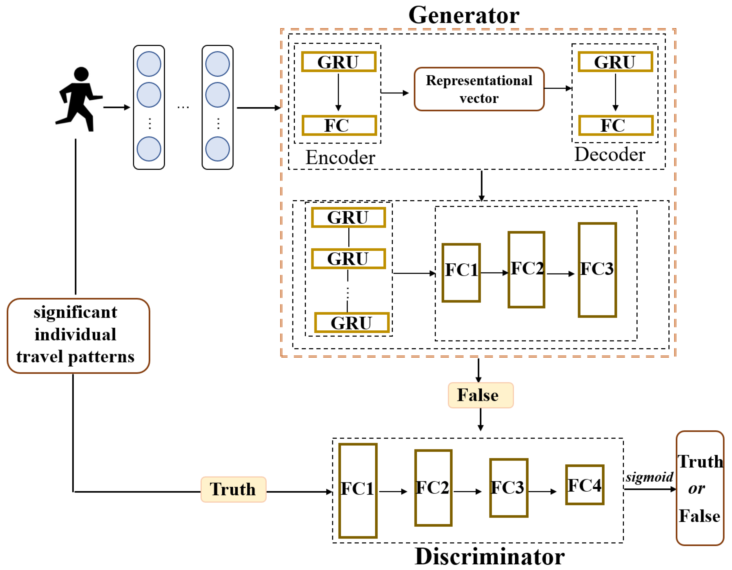
3.5.2. Generative Adversarial Networks Module

The generator network works together with the GRU-based autoencoder to form the generator part of the generative adversarial network, while the discriminator is composed of fully connected layers. The overall design of the model is shown in Figure 3.

As shown in Figure 3, the input to the model is the passenger’s travel chain, i.e., the set of the passenger’s trips. The passenger’s travel chain is sorted in ascending order by trip start time. If the number of trips for the passenger is M and each trip’s feature dimension is N (N = 11), the model’s input is M*N. This is based on the adversarial training approach of the original GAN [2]. The generator part consists of an autoencoder and a pre-trained sub-generator. The purpose of the autoencoder is to capture the representation of the input travel chain information, obtaining the representation result through the embedded layer connected to the encoder. Both the encoder and decoder parts of the autoencoder consist of GRU and FC layers. This design captures the temporal dependencies between passenger trips. The decoder is designed in a structure that mirrors that of the encoder. The passenger’s travel chain vector retains its dimensionality after forward propagation through the autoencoder. This result continues to propagate forward into the pre-trained sub-generator, producing fake values for the GAN to enter the discriminator for true/false judgment. The characteristics of passenger travel times are represented as a probability transition vector in the geographic grid defined in this paper, which is the true value in the model.

The autoencoder and pre-trained sub-generator together form the generator part of the GAN. The samples generated by it are used as fake values in the model training, fed into the discriminator. The construction of the true values for model training was already completed in Section 3.4, representing the travel probability transition vector by placing trips during specific time periods into the defined geographic grid. This vector serves as the model’s true value. The discriminator is constructed using FC layers, with the last layer mapping to a probability within (0, 1) using the Sigmoid function. The closer the probability is to 1, the higher the likelihood that the sample is a real sample, and vice versa. The cross-entropy loss function is used for computation and backpropagation. Aside from using the Sigmoid activation function in the last layer of the discriminator, the Tanh activation function is used in all the other network layers of both the generator and the discriminator.

3.6. Loss Function

The initial generative adversarial network (GAN) employs a multilayer perceptron (MLP) for constructing both the generator (G) and the discriminator (D) [24]. Assuming the dataset used is x, in order for the generator G to learn the distribution, p_g, of x, we first define an input noise for G, which follows the distribution p_z(z). Under the parameter θ_g, the distribution that G can map from the noise z is defined as G (z; θ_g). Similarly, the discriminator D is defined as D (x; θ_d), which represents the probability distribution for the probability that the discriminator can judge the authenticity of the samples under the parameter θ_d. The training of D aims to maximize the accuracy of distinguishing between real samples and the data obtained from G while simultaneously training G to maximize the probability that D classifies the fake samples generated by G as real samples. This is achieved by minimizing the log loss: log(1 − D(G(z))). So the joint loss function, V (G, D), of D and G can be written in the following form:

$$\begin{array}{c}\mathrm{m}\mathrm{i}\mathrm{n}\\ G\end{array}\begin{array}{c}\mathrm{m}\mathrm{a}\mathrm{x}\\ G\end{array}V\left(D,G\right)=E_{x~p_{data}}\left[\log D\left(x\right)\right]+E_{z~p_z\left(x\right)}\left[\log (1-D(G\left(z\right)\left)\right)\right]$$

(6)

Generator G and discriminator D engage in a continuous adversarial game during training until they reach an equilibrium state. At this point, it can be considered that generator G has reached the necessary conditions to simulate the probability distribution of the original data, and it can be assumed that the samples generated by generator G and the original samples both come from the same distribution.

4. Results

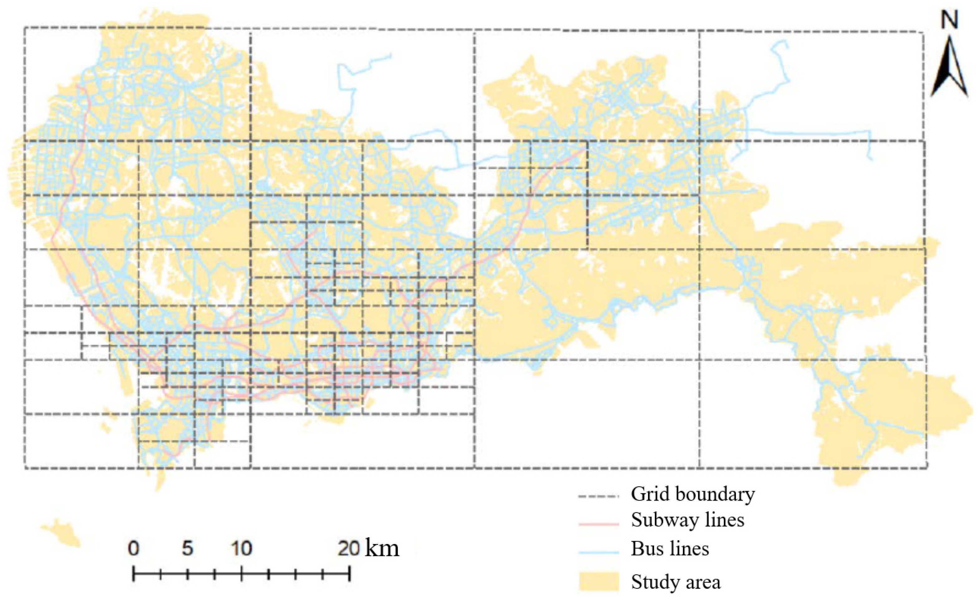
4.1. Data Description and Preprocessing

This study utilizes smart card data from 17 April 2017 to 23 April 2017, covering a one-week period for research purposes. The study area is Shenzhen City, as illustrated in Figure 4. Shenzhen, as one of the forefront cities in China’s development, possesses a vast public transportation network. In April 2017, the public transportation system in Shenzhen primarily comprised 8 subway lines, 199 subway stations, 808 bus routes, and 6226 bus stops, shown as Figure 4.

The data employed in this study include smart card data for Shenzhen’s public transportation (encompassing both subway and bus card data), i.e., public transportation network data. These data sources, originating from different datasets, were transformed into a unified projection coordinate system, WGS 1984 UTM 114E. To enhance computational accuracy, the projection coordinate system was predominantly utilized during the coordinate system calculations. While we initially focused on commuters with exactly two trips per day, we recognize that many commuters may make additional trips after work, for leisure or errands, or work non-standard hours. To account for these behaviors, future analyses could include multiple trips and flexible time windows, allowing for a broader representation of commuting patterns.

This study employs a geographic grid-based method for travel activity pattern representation, which transforms the origin (O) and destination (D) information from travel activities into flows between geographic grids. These inter-grid travel activity flows are referred to as travel activity transitions. The transition probabilities are calculated based on the frequency of these activities, and the probabilities for each location are aggregated into a transition probability vector. This vector serves as the vectorial representation of passenger travel activities.

If the flow within a grid exceeds the maximum flow limit and meets the length constraint for subdivision, the grid is divided into four equal parts. The flow from the original grid is evenly distributed into the four subdivided grids. Similarly, each of these four sub-grids is evaluated for further subdivision. Grids that do not meet the subdivision criteria are included in the set of geographic grids that satisfy the conditions. The study area chosen is Shenzhen City, with data from a single day being utilized for the empirical evaluation. When setting the maximum flow limit to 100,000 and the minimum grid width and height to 2500 m, the resulting grid divisions are shown in Figure 5.

For our empirical evaluation, we chose to use data from 17 April to 23 April 2017 to capture typical travel patterns across a full week, including both weekdays and weekends. This period was selected based on the availability of comprehensive public transportation data for Shenzhen during this time. We acknowledge that public events or anomalies could have affected travel patterns, and we have ensured that no major events (e.g., public holidays or large-scale activities) occurred during this period that would significantly skew the results. However, future studies could benefit from incorporating data from a longer time span to account for broader variations in travel behavior.

Regarding the use of single-day data for gridding, we recognize the limitation of using data from just one day (17 April 2017). While these data were sufficient for a proof-of-concept analysis, we recommend that future studies use data from multiple days or weeks to ensure a more comprehensive and representative model of travel behavior.

4.2. Indicator Description and Empirical Evaluation Configuration

This empirical evaluation is built on a hardware configuration of 64 GB of RAM and NVIDIA-RTX 5000 GPU from NVIDIA, (Santa Clara, CA, USA), using the Windows 10 operating system, torch version 2.1.0 + cuda121, and Pycharm version 2023.2.4 for the empirical evaluation. We employed the Adam optimizer, setting the learning rate for the generator to 0.0001, iterating over the sample set 30 times, and processing 512 input data per iteration. The loss function is BCEloss, as shown in Equation (7).

$$BCE\left(y,y^{\prime }\right)={\displaystyle \frac{{\sum }_{i=1}^n-y_i\mathit{log}{y}_i^{\prime }-\left(1-y_i\right)\mathit{log}(1-y_i^{\prime })}{n}}$$

(7)

4.3. Cluster Analysis of Travel Spatiotemporal Patterns

For both weekdays and weekends, passenger travel data were expressed using the model developed in this study. The resulting low-dimensional compact representations (n = 5) were then subjected to clustering analysis. Inspired by Primerano et al. (2008) [20], the passenger types were categorized into four groups for ease of analysis: (1) Random travelers: these were passengers who took only one trip during the study period. (2) Commuting travelers: These were passengers who made exactly two trips a day, where the first trip started no later than t1(t1 = 10) and the second trip started no earlier than t2(t2 = 17). Additionally, the starting point of the first trip was the same as the endpoint of the second trip, and the time interval between the arrival time of the first trip and the departure time of the second trip exceeded t3(t3 = 8). (3) Short-distance purpose travelers: these were passengers who made exactly two trips a day, excluding commuting trips, where the starting point of the first trip was the same as the endpoint of the second trip. (4) Indeterminate travelers: these were passengers who did not fit into the above three categories.

From

Table 1. Overall analysis.

Category	Number of Passengers	Average Travel Time (min)	Average Number of Stations Passed Through	Average Transfer Times	Random Passengers	Commuting Passengers	Short-Distance Passengers	Indeterminate Passengers
1	2288	40.123	9.877	0.448	0.240	0.307	0.352	0.101
2	1839	42.516	11.183	0.662	0.557	0.214	0.141	0.088
3	5041	33.955	9.137	0.546	0.434	0.196	0.286	0.084
4	2002	34.208	9.266	0.531	0.433	0.202	0.262	0.103
5	681	35.169	9.488	0.543	0.423	0.206	0.268	0.103
Sum	11,851	36.587	9.639	0.542	0.415	0.222	0.271	0.092

, it can be observed that Category 1 includes a higher proportion of commuting passengers and short-distance purpose passengers. Compared to the other categories, these passengers have a longer average travel time, exceeding the average by approximately 5 min. Additionally, they pass through more stations on average and make fewer transfers. The travel characteristic of this category is relatively purpose-driven, opting for more direct travel routes, though the travel time may increase due to factors such as peak hours. Based on this characteristic, it is recommended that this group of people take fast and convenient subway transportation methods, as well as subway lines with fewer transfers and more comfort. Passengers in Category 2 exhibit the longest average travel time, as well as a higher average number of stations passed and a greater average number of transfers. The proportion of random passengers is also higher in this category. These passengers tend to make longer trips with less concern for travel distance and exhibit less regularity in their travel patterns. This group of people can receive personalized recommendations based on their travel destination type and behavioral habits. Categories 3 and 4 show shorter travel times and fewer stations passed compared to the overall average, with a slightly higher proportion of random passengers. These categories primarily consist of short-distance random travelers. This group of people can mainly be recommended subway travel plans with low time costs. Category 5 has the smallest data volume and exhibits high levels of randomness with more complex travel patterns. This group of people can mainly be recommended routes based on their travel purposes and preferences.

A visual analysis of the clustering results is presented in Figure 6. For Category 1’s commuting passengers, the visual analysis reveals that many trips are concentrated in the gray-marked areas of Figure 6. This suggests that the commuting patterns in this category involve round trips within these areas. From an actual map of Shenzhen, it is apparent that these areas are significant transit routes between the city’s central and peripheral regions. Thus, it is inferred that commuting behavior in this category often involves movements between these central and peripheral areas.

Similarly, the visual analysis of long-distance passengers from Category 2 indicates that approximately 30% of these passengers are associated with Shenzhen North Station. Most of these trips originate from Shenzhen North Station (marked by the star in Figure 6) and radiate out to various regions of Shenzhen, as shown by the brown arrows in Figure 5 and Figure 6. This analysis demonstrates that the model captures travel-related features of passenger travel. It identifies clustered travel patterns, such as frequent movements between central and peripheral areas of Shenzhen, which are likely related to the significant activities identified in the adversarial model. Additionally, the model detects local travel activity patterns, such as long-distance travel centered around Shenzhen North Station, suggesting that the model effectively incorporates large-flow areas and group characteristics into its travel activity representation.

Taking the non-working day of 22 April 2017 as an example, 3,093,202 travel itineraries were reconstructed on that day. For ease of analysis, 20,000 travel itineraries were randomly selected for cluster analysis, including 11,661 passengers. Four clusters were selected, and the corresponding indicator results are shown in

Table 2. Cluster analysis of passengers on weekends.

Category	Number of Passengers	Average Travel Time (min)	Average Number of Stations Passed Through	Average Transfer Times	Random Passengers	Commuting Passengers	Short-Distance Passengers	Indeterminate Passengers
1	3506	42. 327	11.971	0.632	0.492	0.103	0.172	0.223
2	4233	30.387	8.812	0.491	0.371	0.172	0.349	0.108
3	3015	34. 835	9.712	0.552	0.432	0.227	0.212	0.129
4	857	35.208	9.466	0.551	0.411	0.213	0.258	0.118
Sum	11,611	35.503	10.047	0.554	0.426	0.168	0.253	0.149

.

The differences between passenger travel on weekends and working days are evident in terms of several aspects. Specifically, the proportion of commuting passengers decreases by approximately 8% on non-working days, while the proportion of passengers in the undetermined category increases by about 5%. This indicates a higher propensity for travel on non-working days, with a corresponding increase in the number of trips and a greater proportion of randomly traveling passengers.

In this study, the classification of travelers into different categories (e.g., commuting, leisure) was based on specific criteria such as trip frequency, timing (e.g., departure and arrival time), and trip purpose (e.g., work-related vs. leisure). For instance, commuting travelers were defined as individuals making exactly two trips per day, one from home to work and one back home again. However, this definition may exclude travelers who take multiple trips per day or those whose work hours that do not fit within the typical 9:00–17:00 timeframe. This could explain the slight 8% decrease in commuting passengers between working and non-working days, as post-work leisure or additional trips (e.g., for errands) may not be captured. Future studies could benefit from more flexible criteria for defining commuting behaviors, such as including multiple trips per day and wider time windows for departure and arrival.

On weekends, long-distance travel behaviors are also present, as illustrated in Category 1 of Table 2. However, in contrast to long-distance travelers on working days (e.g., Category 2 in Table 1), non-working-day long-distance travelers include a lower proportion of commuting and short-distance purpose passengers, with a higher proportion of random travelers. This suggests that long-distance travel on non-working days is more random and less purpose-driven. Based on this characteristic, a subway travel mode suitable for long-distance travel can be recommended for this group of people.

Additionally, as shown in Category 2 of Table 2, short-distance purpose travel on non-working days exhibits a more concentrated behavioral distribution. Consequently, this category demonstrates tighter clustering, indicating that short-distance, purpose-driven travel behaviors are more pronounced on non-working days. This group of people may have a high demand for leisure; therefore, it is recommended that they take public transportation/the subway directly to their destination.

For comparison, 11,851 passengers corresponding to the working day of April 17th were expressed using the original travel chain features and analyzed using hierarchical clustering. They were divided into five categories, as shown in

Table 3. Cluster analysis of passengers on working days.

Category	Number of Passengers	Average Travel Time (min)	Average Number of Stations Passed Through	Average Transfer Times	Random Passengers	Commuting Passengers	Short-Distance Passengers	Indeterminate Passengers
1	6001	36.395	9.568	0.523	0.414	0.233	0.263	0.089
2	1787	36.945	9.722	0.562	0.432	0.206	0.268	0.094
3	2277	36.917	9.773	0.561	0.416	0.196	0.286	0.102
4	768	35.499	9.351	0.541	0.393	0.243	0.274	0.089
5	1018	37.169	9.829	0.573	0.407	0.224	0.288	0.081
Sum	11,851	36.587	9.639	0.542	0.415	0.222	0.271	0.092

.

From the analysis of Table 3, it can be observed that clustering directly based on the features of the original passenger travel chain yields categories with similar analysis metrics across the board, with no significant differences between categories. This is due to the inherent complexity and variability of travel patterns, which make the raw features relatively coarse and less capable of capturing the underlying patterns effectively. As a result, it is challenging to discern different travel activity patterns among passenger categories when using the raw features alone.

The clustering results in Table 2 and Table 3 reveal distinct passenger groups based on their travel behaviors, such as commuting travelers and random travelers, offering valuable insights into how different passenger types utilize the transportation system. These insights can be leveraged to optimize public transportation services, particularly during peak hours, by allocating resources more effectively to high-demand areas.

The travel patterns observed in this study are strongly influenced by the geographical and socioeconomic context of Shenzhen. As a rapidly growing city, Shenzhen’s workforce is diverse, with many residents commuting from outlying districts to the city center. The availability of public transportation options such as buses and subways plays a significant role in shaping travel behavior, particularly on working days when commuters make more predictable trips. On non-working days, travel patterns become more variable, influenced by factors like leisure activities and shopping trips, which are common in Shenzhen’s urban environment.

4.4. Method Comparison and Analysis

Passenger travel is a composite behavior that reflects a complex set of patterns. Additionally, a passenger’s habitual travel behavior can be indicated by their frequently visited travel activity areas. This study aims to estimate the travel activity range of passengers through comparative empirical evaluations. Specifically, the goal is to estimate the top k regions that a given passenger is most likely to visit based on their travel characteristics.

In this estimation process, given a passenger’s travel features x∈X and the entire travel activity range set Q, the task is to determine a subset Y⊆Q containing k elements (where k is less than the total number of elements in Q). The goal is for the probabilities of all elements in Y to be higher than the probabilities of the elements in the complement set S, where S represents the set of elements not included in Y, as shown in Equation (8).

$$P(\forall y\in Y|x)>P(\forall s\in S|x)$$

(8)

Four models are compared for the estimation of travel activity range: (1) the proposed model (Ours), (2) the proposed model without the sub-generator (OursD), (3) the autoencoder-based model (AE), and (4) the model based on raw passenger travel chain features (Raw).

• Proposed model (Ours): this model incorporates the full architecture, including the pre-trained sub-generator, as described in this study.
• Proposed model without sub-generator (OursD): This model is identical to the proposed model except for the omission of the pre-trained sub-generator. It serves to evaluate the impact of the sub-generator on the overall performance of the model.
• Autoencoder-based model (AE): This model uses a standard autoencoder structure, where both the encoder and decoder are composed of GRU layers and fully connected layers. The central embedding layer serves as a reference for the compact representation. The AE model is used to assess the effectiveness of conventional deep learning feature compression methods.
• Raw travel chain feature model (Raw): This model utilizes the raw travel chain features, as described in Section 3.2. Given that a passenger may take multiple trips, these are aggregated by averaging them to form a single composite vector. This model is used to validate the effectiveness of direct feature expression.
• Collaborative filtering (CF): this is a popular method used in recommendation systems, where the goal is to suggest items (e.g., products, services, or in this case, travel routes) based on the preferences of similar users.
• Spatiotemporal clustering (STC): This is a technique used to group data points based on both spatial (location) and temporal (time) dimensions. This method is particularly useful in contexts where data are influenced by both where an event occurs and when it happens, such as in urban transportation systems, weather patterns, or social media trends.

These four models provide different approaches for expressing passenger travel chain features, leading to varying representations. Consequently, when used as input features for the travel activity range estimation model, each model exhibits distinct characteristics. The estimation model is designed as a fully connected neural network comprising four layers, with neuron configurations of (input dimension, 20), (20, 40), (40, 70), and (70, output dimension), respectively. The activation function used is the Sigmoid function. The loss function for this model is cross-entropy loss (CEL), as defined in Equation (9). In the training phase, for each passenger, k training samples are created, representing the k most frequently visited regions. To account for the frequency differences among these regions, the training sample set is constructed in the proportion k:k − 1:…:2:1, with a higher proportion allocated to regions with higher visitation probabilities. After training, the top k regions with the highest output probabilities are selected as the estimated most frequently visited travel activity areas for the passenger.

$$CEL\left(x,label\right)=-\mathit{log}{\displaystyle \frac{e^{x}label}{{\sum }_{j=1}^n{e}^{x}j}}$$

(9)

Following the design of evaluation metrics used in retrieval ranking models, two metrics are employed to assess the performance of the comparison models: Average Relevance (AR, Equation (10)) and Average Precision (AP, Equation (11)). In this study, Average Relevance (AR) and Average Precision (AP) are particularly useful for assessing how well the model captures and ranks individualized travel patterns. Since the goal is to make personalized travel recommendations, these metrics help evaluate whether the model provides relevant and high-quality suggestions for each passenger. AP emphasizes the accuracy of the top recommendations, ensuring that the most relevant travel behaviors are prioritized. AR, on the other hand, assesses the overall relevance of the entire set of predictions, ensuring that the model does not just focus on ranking the top predictions but also captures the full range of distinct travel behaviors:

$$AR={\displaystyle \frac{{\sum }_{i=1}^N\raisebox{1ex}{$\sum _{j=1}^k{I}_y\left(y_j^{\prime }\right)$}\!\left/ \!\raisebox{-1ex}{$k$}\right.}{N}}$$

(10)

$$Ap={\displaystyle \frac{{\sum }_i^N\raisebox{1ex}{$\sum _{j=1}^k{I}_{yj}\left(y_j^{\prime }\right)$}\!\left/ \!\raisebox{-1ex}{$k$}\right.}{N}}$$

(11)

$$I_y\left(x\right)=\left\{\begin{array}{c}1, x\in y\\ 0, x\notin y\end{array}\right.$$

(12)

We selected k = 3 and k = 5 for comparative empirical evaluations. We used a total of 4 working days from 18 April to 21 April as the training data for the sunrise chain and selected data from 17 April for testing. The comparative empirical results are shown in

Table 4. Comparison results.

Methods	AR (k = 3)	AP (k = 3)	AR (k = 5)	AP (k = 5)
Raw	0.626	0.553	0.595	0.527
AE	0.637	0.551	0.609	0.531
CF	0.596	0.532	0.586	0.501
STC	0.620	0.544	0.598	0.529
OursD	0.707	0.594	0.674	0.562
Ours	0.723	0.637	0.709	0.581

.

From Table 4, it can be observed that there is little difference in the performance metrics between the original features and the features obtained through autoencoder training. The models that exclude the sub-generator (OursD) and the full model (Ours) show relatively better evaluation results. The pre-trained sub-generator in the full model enhances convergence and results in a noticeable improvement in the evaluation metrics. Further analysis indicates that the autoencoder primarily serves the purpose of feature compression, resulting in a compact representation of the original features without incorporating additional information. As a result, the performance of the autoencoder model is similar to that of the original features.

The introduction of the generative adversarial network (GAN) for data representation, through adversarial training to approximate the true data distribution and incorporating certain constraints to guide convergence, explains why the latter two models show improved evaluation metrics. Specifically, the full model with the pre-trained sub-generator achieves higher performance compared to the model without the sub-generator. Furthermore, we introduce the use of generative adversarial networks (GANs) to model the distribution of passenger travel patterns, which allows us to generate compact and high-level representations of travel behavior. This methodology enables us to not only understand individual travel patterns but also simulate potential future behaviors, providing valuable insights for urban transportation planning.

As shown in Figure 7, a comparison between the feature representation of our model and the original travel chain features was conducted using the travel activity range results for some commuting passengers from Category 1 in Table 3. It was found that for passengers with inaccurate estimated ranges, such as passengers with a travel activity range in Region G, the results using the original travel chain features often lacked consistency, estimating regions like A, C, and E, whereas the results from our model frequently identified Region B. This is because Regions B and G are both densely populated commuting areas, despite differing in terms of geographical location. Our model, by incorporating significant individual activities, provides a more compact and similar vector representation for commuting passengers, capturing high-level travel-related information better than the original feature representation. However, there remains some deviation, indicating that while the model captures commuting travel behavior-related information, the spatial information captured is still imprecise, suggesting room for improvement in absolute accuracy. This may be due to the algorithm used for grid partitioning, which needs further refinement to consider more spatiotemporal heterogeneity, as well as the relatively simple architecture of the fully connected layers in the travel activity estimation model, which could benefit from enhancement.

For passengers starting from Regions D and F, located in densely populated areas within Shenzhen, all the models showed inaccurate travel activity range estimates. This is likely due to the complexity and randomness of travel behavior in these densely connected and high-traffic areas. This suggests that the model still requires improvements. While comparative empirical evaluations emphasize relative metrics, there is still a need for further refinement of the models to enhance absolute accuracy in these evaluations.

The high-level travel profiles generated through our method (illustrated in Figure 7) can be used to create personalized travel recommendations for passengers. For example, commuters could be advised on the best time to take public transport based on their usual travel patterns, thus improving the passenger experience and reducing congestion during peak hours.

5. Conclusions and Discussion

The study of human travel activities is crucial for analyzing behavioral habits, understanding urban socioeconomic structures, assisting in urban planning and design, and for municipal construction. The daily generation of passenger travel trajectory data from smart public transportation systems and travel platforms provides a solid data foundation for researching human mobility. This paper, by examining the advantages and limitations of classical human travel activity models from a statistical perspective and existing data-driven representation models, proposes a travel representation method for individual bus passengers based on generative adversarial networks (GANs). In contrast, the model proposed in this study offers a more refined representation of passenger travel patterns by incorporating significant individual travel modes and employing adversarial training through generative adversarial networks (GANs) to capture the distribution of passenger travel. This approach allows the model to better identify and capture similar travel patterns among passengers compared to clustering based on raw travel chain features. Nevertheless, since individual travel activities are inherently complex, the proposed model provides a significantly improved representation compared to the original model, leading to greater differentiation in clustering results. This means that passengers with similar travel behaviors are represented more closely in the high-dimensional space of the model. However, there remains substantial room for improvement in terms of absolute accuracy in the representation. Our findings, particularly the identification of distinct travel patterns, have significant implications for urban transportation planning. By understanding the spatiotemporal distribution of passenger demand, city planners can make more data-driven decisions about infrastructure improvements, ensuring that the transportation network meets the evolving needs of urban residents. This study’s results provide a foundation for developing smart transportation systems capable of adapting to individual passenger needs. By understanding travel behaviors and offering personalized travel suggestions, cities can improve the efficiency and quality of public transport, reducing congestion and environmental impact. While this study uses data from the entire public transportation system, the personalized travel representation method proposed here is specifically applied to individual bus passengers. Future work could expand this approach to other transportation modes, such as subway or ferries, to provide a more comprehensive model for urban travel behavior.

However, there are some limitations in this work, which can inspire future research: (1) refinement of passenger travel chain features: This study models passenger travel chains based on spatiotemporal constraints. Nevertheless, there is a need for more detailed modeling of travel chain features. It is necessary to extract the functional areas, passenger travel purposes, and social attributes of the departure and arrival destinations in order to improve the prediction accuracy more finely. On the other hand, passengers who pay using cash or alternative methods are excluded from the dataset, which may lead to a skewed representation of travel behaviors, particularly for certain demographic groups. Additionally, data gaps due to technical errors or incomplete journeys may affect the accuracy of travel behavior profiling. Future work could consider combining smart card data with other data sources, such as survey data or mobile phone data, to address these gaps and provide a more comprehensive overview of travel behavior across all passenger groups. (2) Optimization of generative adversarial networks: This work primarily focuses on improving the generator component of the GAN, while the discriminator still employs fully connected layers. Future improvements should include advancements in the discriminator part. Additionally, exploring variations of GANs, such as Deep Convolutional GANs or Conditional GANs, represents a promising direction for optimizing the model. (3) Integration of multi-source socioeconomic data and comparison among different cities: Incorporating socioeconomic data among different cities such as housing prices, land use, and population statistics into the modeling process could enhance both the accuracy and practical relevance of the model. (4) Future work could extend this analysis by incorporating data from multiple weeks and refining the grid division to account for seasonal or event-based variations. This would not only improve the precision of predictions but also increase the model’s applicability and value in real-world scenarios.

References

1. Li, Y.; Yang, G.; Su, Z.; Li, S.; Wang, Y. Human activity recognition based on multienvironment sensor data. Inf. Fusion 2023, 91, 47–63. [Google Scholar] [CrossRef]
2. Barabási, A.-L. The origin of bursts and heavy tails in human dynamics. Nature 2005, 435, 207–211. [Google Scholar] [CrossRef]
3. Brockmann, D.; Lars, H.; Theo, G. The scaling laws of human travel. Nature 2006, 439, 462–465. [Google Scholar] [CrossRef]
4. Barbosa, H.; Barthelemy, M.; Ghoshal, G.; James, C.R.; Lenormand, M.; Louail, T.; Menezes, R.; Ramasco, J.J.; Simini, F.; Tomasini, M. Human mobility: Models and applications. Phys. Rep. 2018, 734, 1–74. [Google Scholar] [CrossRef]
5. Shi, Y.; Zheng, Y.; Chen, D.; Yang, J.; Cao, Y.; Cui, A. Research on the Correlation between the Dynamic Distribution Patterns of Urban Population Density and Land Use Morphology Based on Human–Land Big Data: A Case Study of the Shanghai Central Urban Area. Land 2024, 13, 1547. [Google Scholar] [CrossRef]
6. Ray, A.; Kolekar, M.H.; Balasubramanian, R.; Hafiane, A. Transfer learning enhanced vision-based human activity recognition: A decade-long analysis. Int. J. Inf. Manag. Data Insights 2022, 3, 100142. [Google Scholar] [CrossRef]
7. Li, X.; Lu, Z. Spatiotemporal Evolution of Land Use Structure and Function in Rapid Urbanization: The Case of the Beijing–Tianjin–Hebei Region. Land 2024, 13, 1651. [Google Scholar] [CrossRef]
8. Xu, Y.; Belyi, A.; Bojic, I.; Ratti, C. Human mobility and socioeconomic status: Analysis of Singapore and Boston. Comput. Environ. Urban Syst. 2018, 72, 51–67. [Google Scholar] [CrossRef]
9. Song, C.; Qu, Z.; Blumm, N.; Barabási, A.-L. Limits of predictability in human mobility. Science 2010, 327, 1018–1021. [Google Scholar] [CrossRef]
10. Zipf, G.K. The P 1 P 2/D hypothesis: On the intercity movement of persons. Am. Sociol. Rev. 1946, 11, 677–686. [Google Scholar] [CrossRef]
11. Simini, F.; González, M.C.; Maritan, A.; Barabási, A.-L. A universal model for mobility and migration patterns. Nature 2012, 484, 96–100. [Google Scholar] [CrossRef] [PubMed]
12. Masucci, A.P.; Serras, J.; Johansson, A.; Batty, M. Gravity versus radiation models: On the importance of scale and heterogeneity in commuting flows. Phys. Rev. E Stat. Nonlinear Soft Matter Phys. 2013, 88, 022812. [Google Scholar] [CrossRef] [PubMed]
13. Gordon, J.B.; Koutsopoulos, H.N.; Wilson, N.H.M.; Attanucci, J.P. Automated inference of linked transit journeys in london using fare-transaction and vehicle location data. Transp. Res. Rec. 2013, 2343, 17–24. [Google Scholar] [CrossRef]
14. Mikolov, T.; Sutskever, I.; Chen, K.; Corrado, G.S.; Dean, J. Distributed representations of words and phrases and their compositionality. Adv. Neural Inf. Process. Syst. 2013, 26, 1–9. [Google Scholar]
15. Wang, P.; Fu, Y.; Xiong, H.; Li, X. Adversarial substructured representation learning for mobile user profiling. In Proceedings of the 25th ACM SIGKDD International Conference on Knowledge Discovery & Data Mining, Anchorage, AK, USA, 4–8 August 2019. [Google Scholar]
16. Gao, Q.; Zhou, F.; Zhang, K.; Trajcevski, G.; Luo, X.; Zhang, F. Identifying Human Mobility via Trajectory Embeddings. Twenty-Sixth International Joint Conference on Artificial Intelligence. In Proceedings of the Twenty-Sixth International Joint Conference on Artificial Intelligence Melbourne Australia, 19–25 August 2017; Volume 17. [Google Scholar]
17. Dai, Q.; Li, Q.; Tang, J.; Wang, D. Adversarial network embedding. In Proceedings of the AAAI Conference on Artificial Intelligence, New Orleans, LA, USA, 2–7 February 2018; Volume 32. No. 1. [Google Scholar]
18. Gong, S.; Dong, X.; Wang, K.; Lei, B.; Jia, Z.; Qin, J.; Roadknight, C.; Liu, Y.; Cao, R. Agent-based modelling with geographically weighted calibration for intra-urban activities simulation using taxi GPS trajectories. Int. J. Appl. Earth Obs. Geoinf. 2023, 122, 103368. [Google Scholar] [CrossRef]
19. Mor, M.; Dalyot, S.; Ram, Y. Who is a tourist? Classifying international urban tourists using machine learning. Tour. Manag. 2022, 95, 104689. [Google Scholar] [CrossRef]
20. Primerano, F.; Taylor, M.A.; Pitaksringkarn, L.; Tisato, P. Defining and understanding trip chaining behavior. Transportation 2008, 35, 55–72. [Google Scholar] [CrossRef]
21. Yang, H.; Wang, L.; Tang, F.; Fu, M.; Xiong, Y. Differences in Urban Vibrancy Enhancement among Different Mixed Land Use Types: Evidence from Shenzhen, China. Land 2024, 13, 1661. [Google Scholar] [CrossRef]
22. Zhou, F.; Yin, R.; Zhang, K.; Trajcevski, G.; Zhong, T.; Wu, J. Adversarial point-of-interest recommendation. In Proceedings of the The World Wide Web Conference, Raleigh, NC, USA, 26–30 April 2010. [Google Scholar]
23. Chen, C.; Liao, C.; Xie, X.; Wang, Y.; Zhao, J. Trip2Vec: A deep embedding approach for clustering and profiling taxi trip purposes. Pers. Ubiquitous Comput. 2018, 23, 53–66. [Google Scholar] [CrossRef]
24. Goodfellow, I.; Pouget-Abadie, J.; Mirza, M.; Xu, B.; Warde-Farley, D.; Ozair, S.; Courville, A.; Bengio, Y. Generative Adversarial Nets, NIPS. 2014. Available online: https://proceedings.neurips.cc/paper_files/paper/2014/hash/5ca3e9b122f61f8f06494c97b1afccf3-Abstract.html (accessed on 10 October 2024).
25. Wang, H.; Wang, J.; Wang, J.; Zhao, M.; Zhang, W.; Zhang, F.; Xie, X.; Guo, M. Graphgan: Graph representation learning with generative adversarial nets. In Proceedings of the AAAI Conference on Artificial Intelligence, New Orleans, LA, USA, 2–7 February 2018; Volume 32. No. 1. [Google Scholar]
26. Zhou, F.; Yin, R.; Zhang, K.; Trajcevski, G.; Zhong, T.; Wu, J. Adversarial point-of-interest recommendation. In Proceedings of the WWW ‘19: The Web Conference, San Francisco, CA, USA, 13–17 May 2019. [Google Scholar]
27. Gao, Q.; Zhang, F.; Yao, F.; Li, A.; Mei, L.; Zhou, F. Adversarial mobility learning for human trajectory classification. IEEE Access 2020, 8, 20563–20576. [Google Scholar] [CrossRef]
28. Lasinio, G.J.; Santoro, M.; Mastrantonio, G. CircSpaceTime: An R package for spatial and spatio-temporal modelling of circular data. J. Stat. Comput. Simul. 2020, 90, 1315–1345. [Google Scholar] [CrossRef]
29. Agrawal, R. Gast Algorithm for Mining Association Rules in Large Databases. In Proceedings of the 20th Very Large Data Bases Conference, Santiago de, Chile, Chile, 12–15 September 1994. [Google Scholar]
Figure 1. Algorithm flowchart.
Land 13 02178 g001
Figure 2. Pre-training process.
Land 13 02178 g002
Figure 3. Passenger profile construction supported by generative adversarial networks.
Land 13 02178 g003
Figure 4. Study area.
Land 13 02178 g004
Figure 5. Quadtree partition grid diagram.
Land 13 02178 g005
Figure 6. Characteristics of travel groups.
Land 13 02178 g006
Figure 7. Spatial distribution patterns of different types of populations (A, C and E represent random mobility area, B and G represent high-traffic commuter area, D and F represent areas with intensive travel activities).
Land 13 02178 g007