
A Geospatial Decision Support System for Supporting the Assessment of Land Degradation in Europe

 ,
,  ,
,  and
and
Abstract
1. Introduction
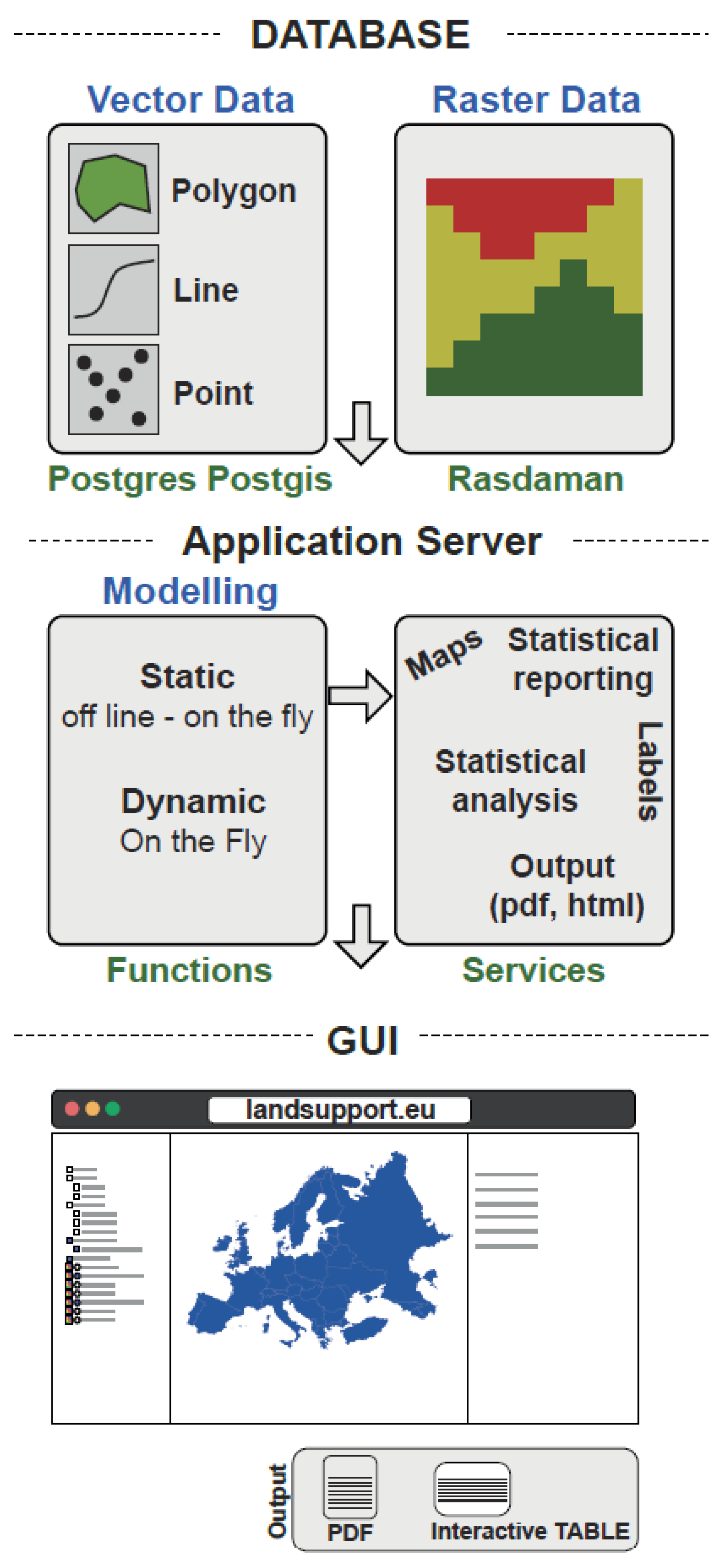
The LANDSUPPORT Platform
2. Materials and Methods
The SDG 15.3.1 Indicator
3. Results
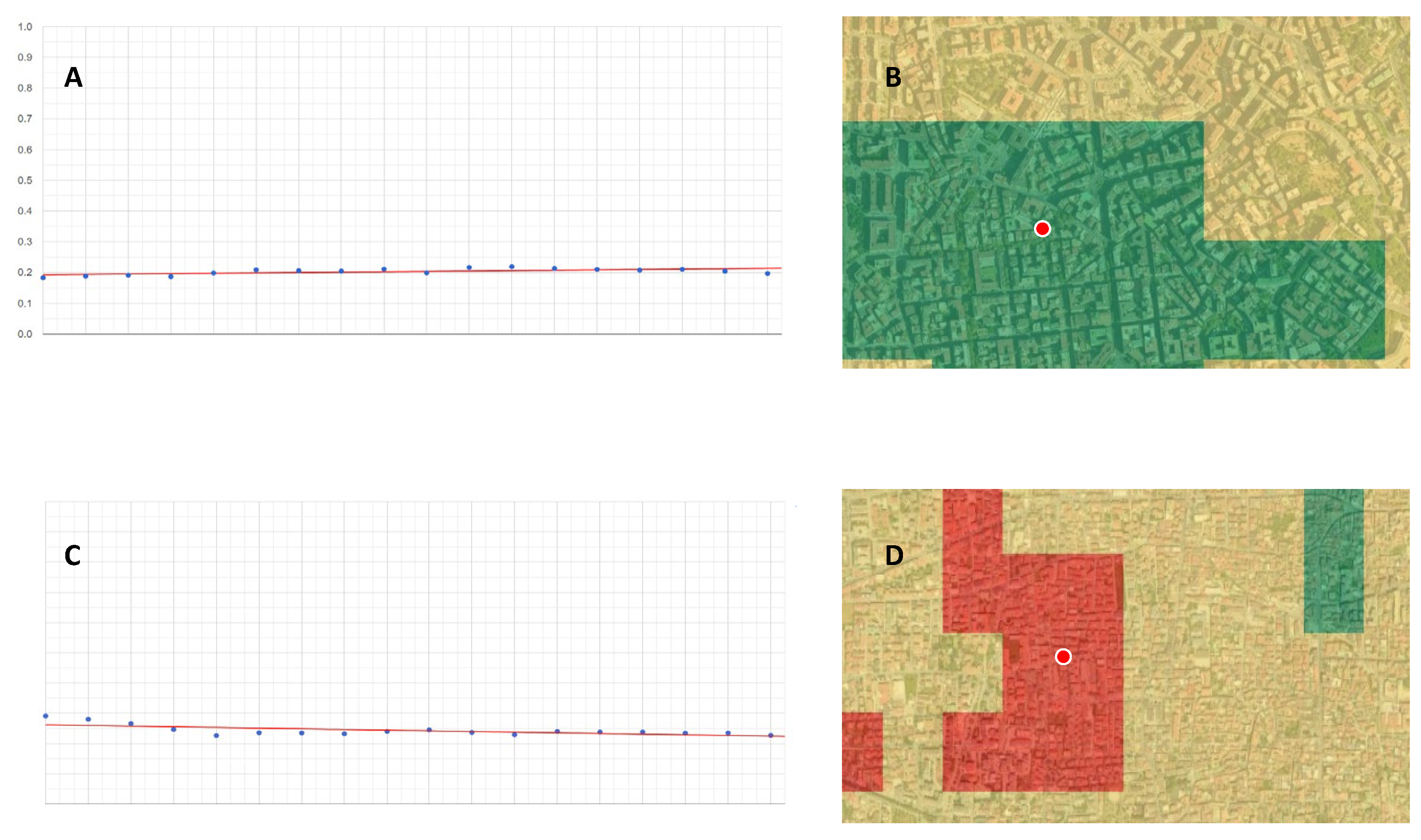
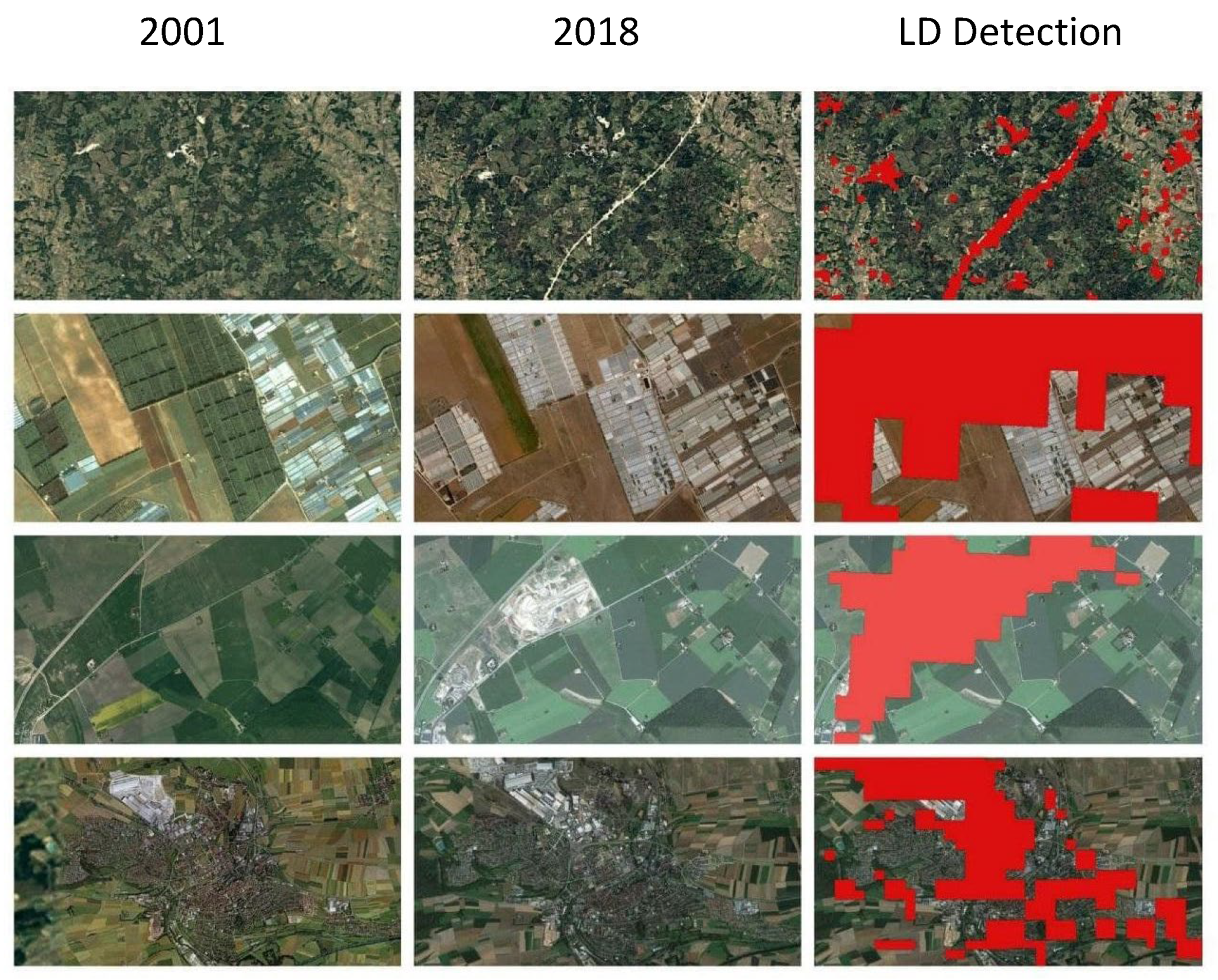
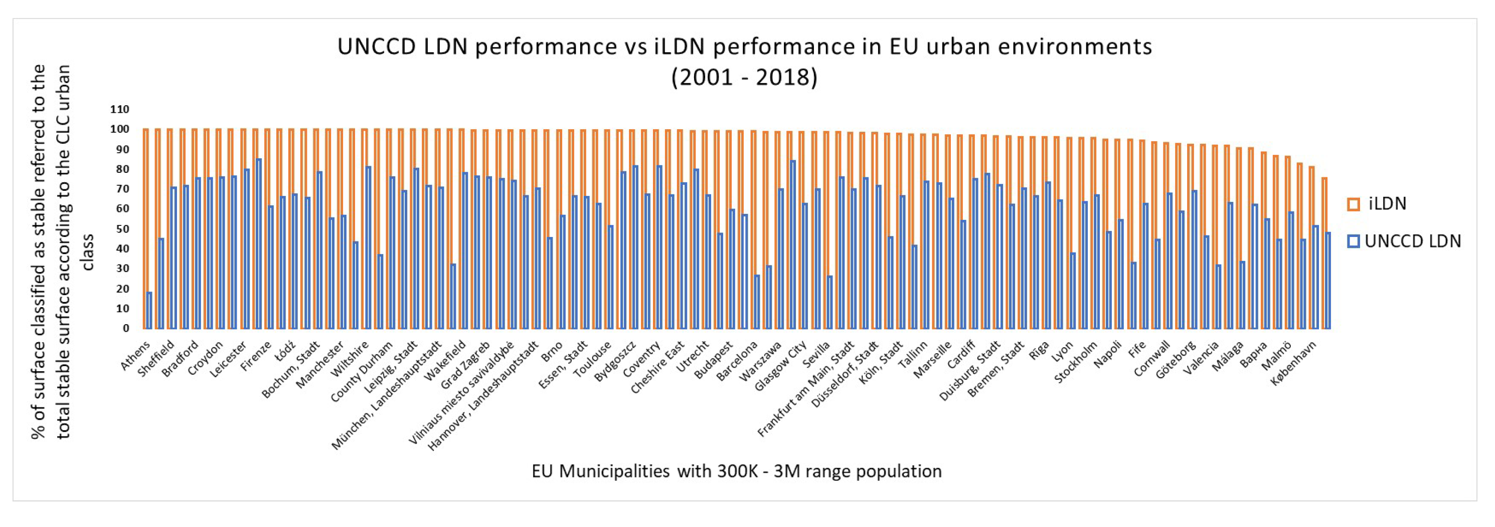
3.1. Indicator Test, Verification and Improvement
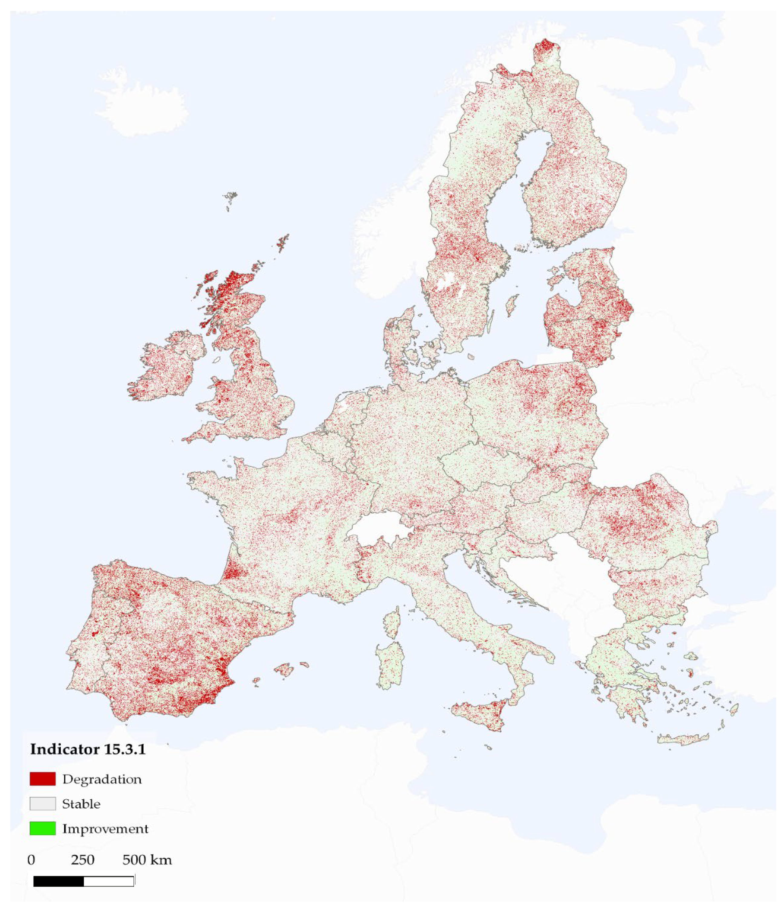
3.2. The Improved SDG 15.3.1 Indicator
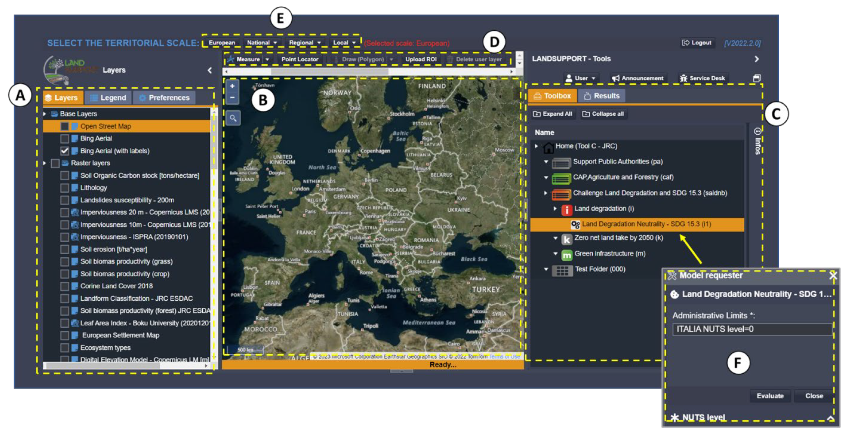
3.3. The LDN Tool
4. Case Studies
4.1. Case 1: (National Extension)
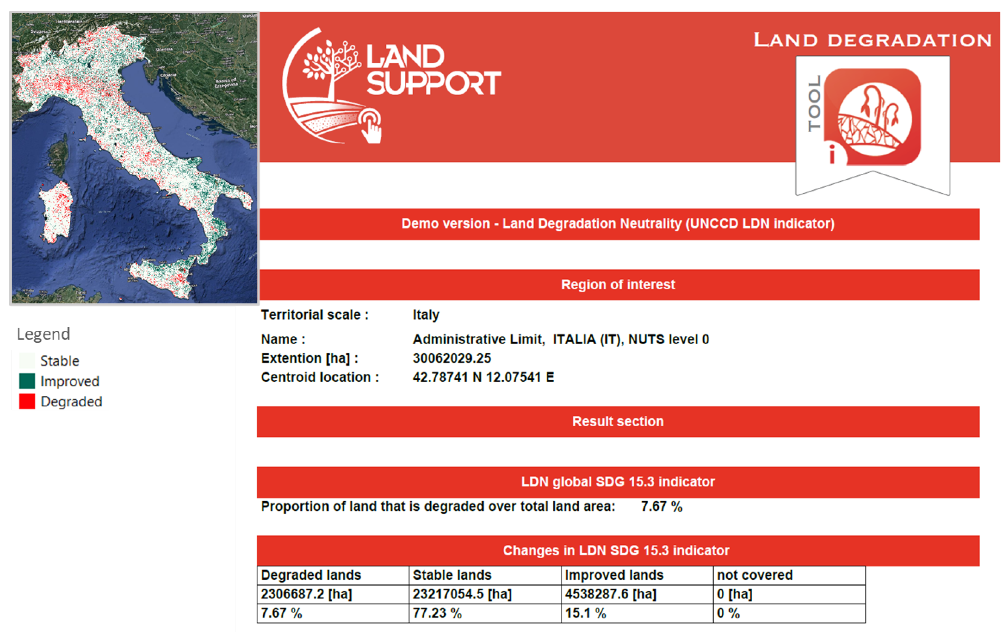
4.1.1. Obtaining the SDG Indicator 15.3.1 at the National Level
LANDSUPPORT Tool Help
4.2. Case 2: (Regional Extension)
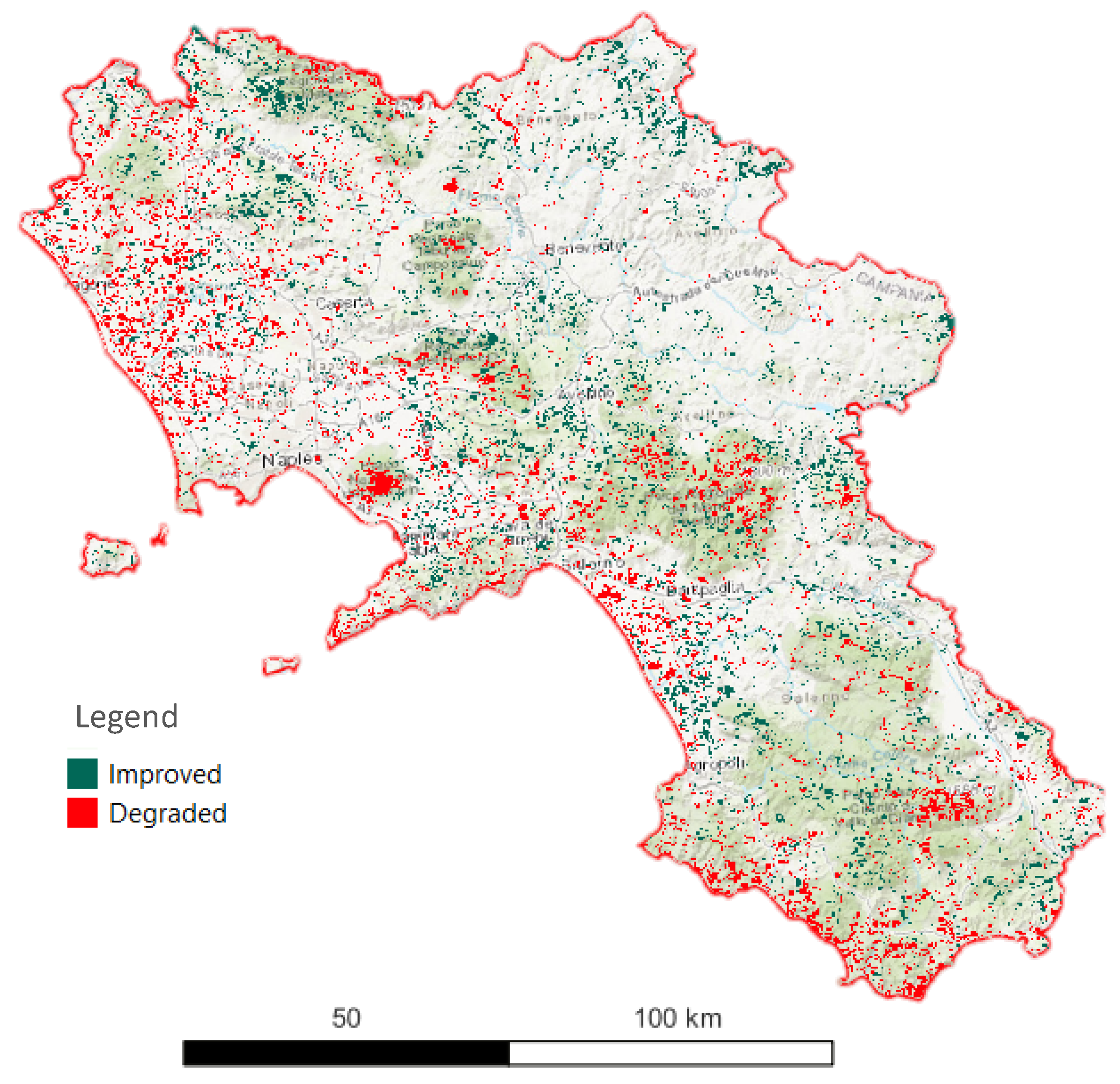
4.2.1. Improving the Regional Rural Development Plan
LANDSUPPORT Tool Help
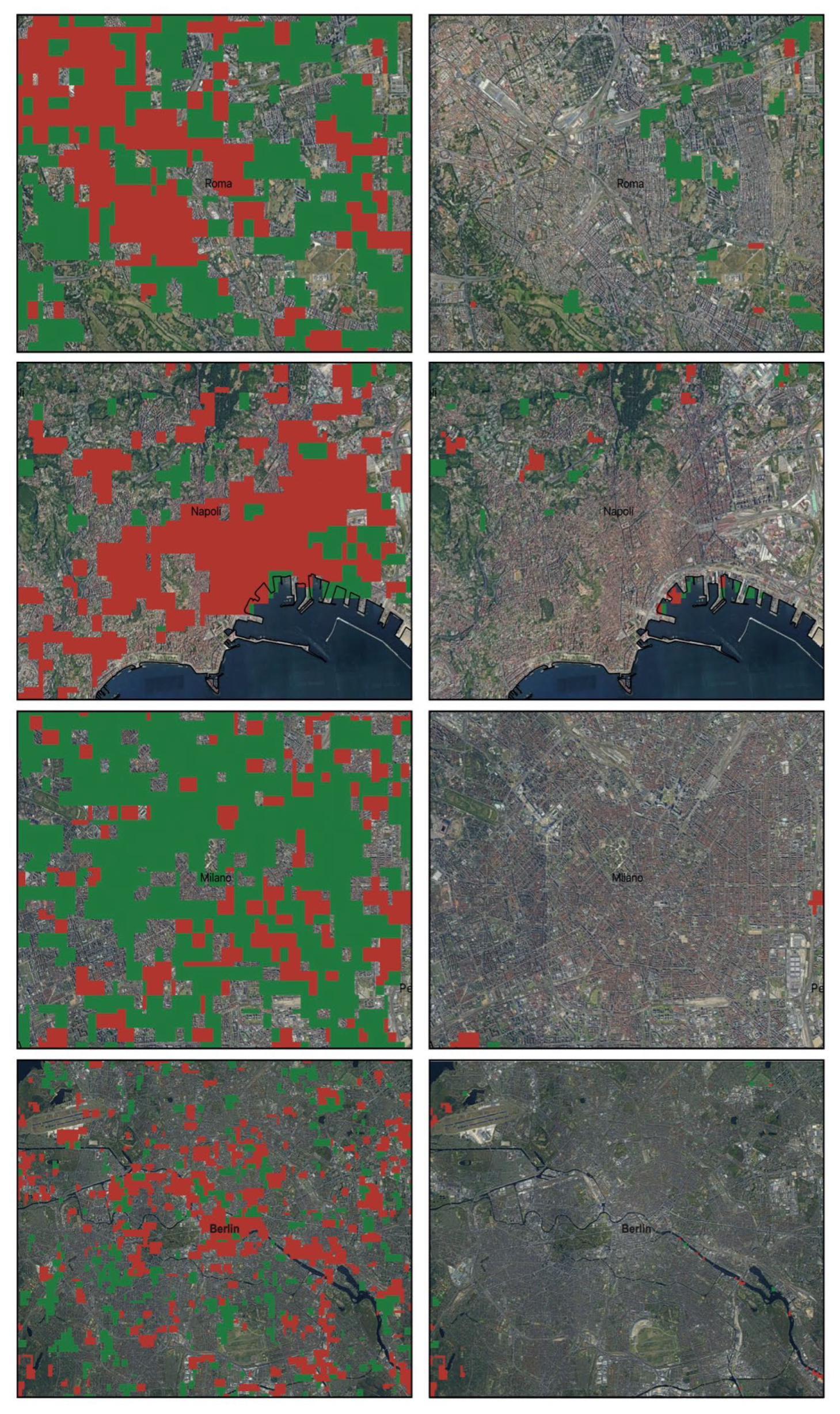
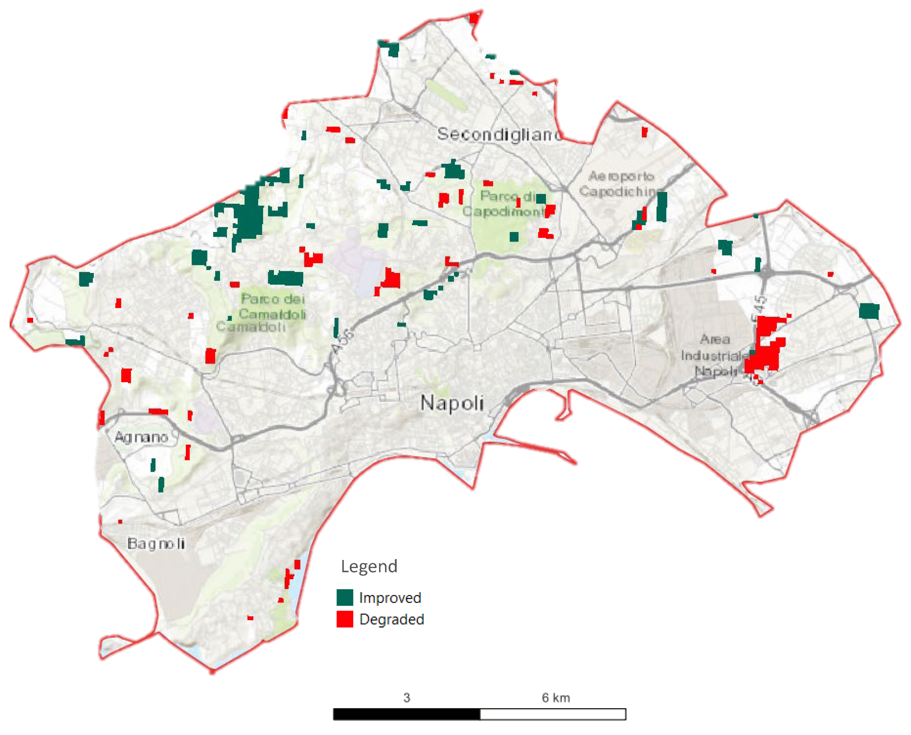
4.3. Case 3: (Municipalities)
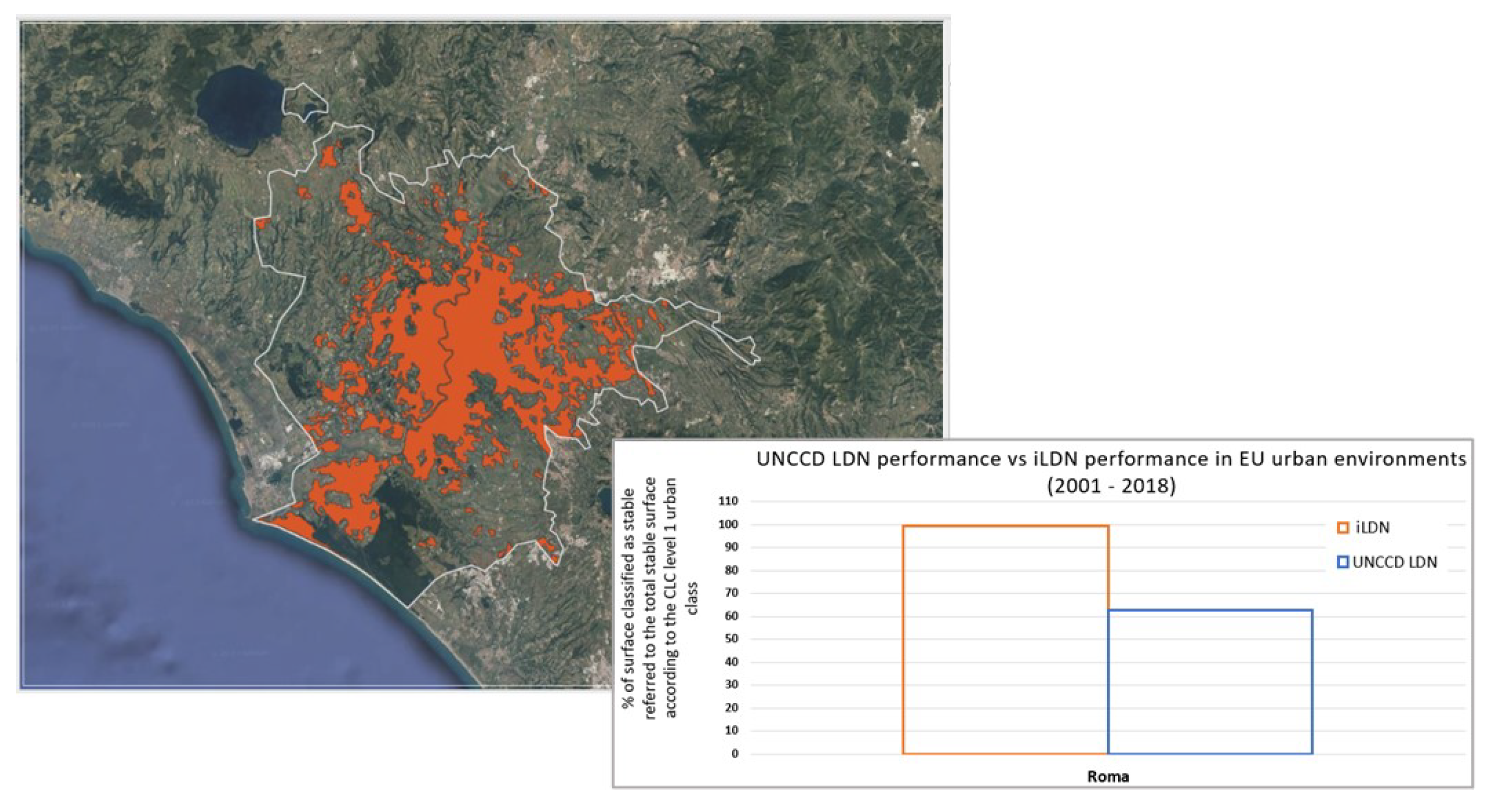
4.3.1. Updating the Municipal Urbanization Plan (PUC) of the Naples Municipality
LANDSUPPORT Tool Help
5. Discussion
6. Conclusions
Author Contributions
Funding
Data Availability Statement
Acknowledgments
Conflicts of Interest
References
- Koch, A.; Mcbratney, A.; Adams, M.; Field, D.; Hill, R.; Crawford, J.; Minasny, B.; Lal, R.; Abbott, L.; O’Donnell, A.; et al. Soil Security: Solving the Global Soil Crisis. Glob. Policy 2013, 4, 434–441. [Google Scholar] [CrossRef]
- Lal, R. Soil carbon sequestration impacts on global climate change and food security. Science 2004, 304, 1623–1627. [Google Scholar] [CrossRef]
- IPBES. The IPBES Assessment Report on Land Degradation and Restoration; Montanarella, L., Scholes, R., Brainich, A., Eds.; Secretariat of the Intergovernmental Science-Policy Platform on Biodiversity and Ecosystem Services: Bonn, Germany, 2018; 744p. [Google Scholar] [CrossRef]
- Weber, J. Accounting for soil in the SEEA. In Proceedings of the 12th Meeting of the London Group on Environmental Accounting, Rome, Italy, 17–19 December 2007. [Google Scholar]
- Wilkki, M.; Reeve, N. European Missions Overview. Communication from the Commission to the European Parliament, the Council, the European Economic and Social Committee and the Committee of the Regions on European Missions, Brussels, 29.9.2021 COM(2021) 609 Final 2021. Available online: https://op.europa.eu/en/publication-detail/-/publication/7e2fad00-2716-11ec-bd8e-01aa75ed71a1/language-en (accessed on 5 April 2023).
- Tóth, G.; Hermann, T.; da Silva, M.R.; Montanarella, L. Monitoring soil for sustainable development and land degradation neutrality. Environ. Monit. Assess. 2018, 190, 57. [Google Scholar] [CrossRef]
- Sims, N.C.; Green, C.; Newnham, G.J.; England, J.R.; Held, A.; Wulder, M.A.; Herold, M.; Cox, S.J.D.; Huete, A.R.; Kumar, L.; et al. Good Practice Guidance. SDG Indicator 15.3.1. Proportion of Land That Is Degraded over Total Land Area; UNCCD-SPI: Bonn, Germany, 2017; Available online: https://www.unccd.int/sites/default/files/relevant-links/2017-10/Good%20Practice%20Guidance_SDG%20Indicator%2015.3.1_Version%201.0.pdf (accessed on 5 April 2023).
- Orr, B.J.; Cowie, A.L.; Castillo Sanchez, V.M.; Chasek, P.; Crossman, N.D.; Erlewein, A.; Louwagie, G.; Maron, M.; Metternicht, G.I.; Minelli, S.; et al. Scientific Conceptual Framework for Land Degradation Neutrality. A Report of the Science-Policy InterfAce; United Nations Convention to Combat Desertification (UNCCD): Bonn, Germany, 2017. [Google Scholar]
- Conservation International. Trends.Earth 1.0.7 Documentation. 2018. Available online: https://docs.trends.earth/en/latest/ (accessed on 10 May 2023).
- Xoxo, S.; Mantel, S.; de Vos, A.; Mahlaba, B.; le Maître, D.; Tanner, J. Towards SDG 15.3: The biome context as the appropriate degradation monitoring dimension. Environ. Sci. Policy 2022, 136, 400–412. [Google Scholar] [CrossRef]
- Feng, S.; Zhao, W.; Zhan, T.; Yan, Y.; Pereira, P. Land degradation neutrality: A review of progress and perspectives. Ecol. Indic. 2022, 144, 109530. [Google Scholar] [CrossRef]
- Ding, Z.; Peng, J.; Qiu, S.; Zhao, Y. Nearly Half of Global Vegetated Area Experienced Inconsistent Vegetation Growth in Terms of Greenness, Cover, and Productivity. Earth’s Future 2020, 8, e2020EF001618. [Google Scholar] [CrossRef]
- Baret, F.; Guyot, G. Potentials and limits of vegetation indices for LAI and APAR assessment. Remote Sens. Environ. 1991, 35, 161–173. [Google Scholar] [CrossRef]
- Cui, Y.; Li, X. A new global land productivity dynamic product based on the consistency of various vegetation biophysical indicators. Big Earth Data 2022, 6, 36–53. [Google Scholar] [CrossRef]
- Ivits, E.; Horion, S.; Erhard, M.; Fensholt, R.; Penuelas, J. Assessing European ecosystem stability to drought in the vegetation growing season. Glob. Ecol. Biogeogr. 2016, 25, 1131–1143. [Google Scholar] [CrossRef]
- Paredes-Trejo, F.; Barbosa, H.; Giovannettone, J.; Kumar, T.V.L.; Kumar Thakur, M.; de Oliveira Buriti, C. Drought variability and land degradation in the Amazon River basin. Front. Earth Sci. 2022, 10, 939908. [Google Scholar] [CrossRef]
- Lorenz, K.; Lal, R.; Ehlers, K. Soil organic carbon stock as an indicator for monitoring land and soil degradation in relation to United Nations’ Sustainable Development Goals. Land Degrad. Dev. 2019, 30, 824–838. [Google Scholar] [CrossRef]
- Al Sayah, M.J.; Abdallah, C.; Sarkissian, R.D.; Abboud, M. A framework for investigating the land degradation neutrality-Disaster risk reduction nexus at the sub-national scales. J. Arid Environ. 2021, 195, 104635. [Google Scholar] [CrossRef]
- Prince, S.D. Challenges for remote sensing of the Sustainable Development Goal SDG 15.3.1 productivity indicator. Remote Sens. Environ. 2019, 234, 111428. [Google Scholar] [CrossRef]
- Schillaci, C.; Jones, A.; Vieira, D.; Munafò, M.; Montanarella, L. Evaluation of the Sustainable Development Goal 15.3.1 Indicator of Land Degradation in the European Union. Land Degrad. Dev. 2022, 34, 250–268. [Google Scholar] [CrossRef]
- Olsson, L.; Barbosa, H.; Bhadwal, S.; Cowie, A.; Delusca, K.; Flores-Renteria, D.; Hermans, K.; Jobbagy, E.; Kurz, W.; Li, D.; et al. Land Degradation. In Climate Change and Land: An IPCC Special Report on Climate Change, Desertification, Land Degradation, Sustainable Land Management, Food Security, and Greenhouse Gas Fluxes in Terrestrial Ecosystems; Shukla, P.R., Skea, J., Buendia, E.C., Masson-Delmotte, V., Pörtner, H.-O., Roberts, D.C., Zhai, P., Slade, R., Connors, S., van Diemen, R., et al., Eds.; IPCC: Geneva, Switzerland, 2019. [Google Scholar] [CrossRef]
- GreGiuliani, G.; Mazzetti, P.; Santoro, M.; Nativi, S.; Van Bemmelen, J.; Colangeli, G.; Lehmann, A. Knowledge generation using satellite earth observations to support sustainable development goals (SDG): A use case on Land degradation. Int. J. Appl. Earth Obs. Geoinf. 2020, 88, 102068. [Google Scholar] [CrossRef]
- Von Maltitz, G.P.; Gambiza, J.; Kellner, K.; Rambau, T.; Lindeque, L.; Kgope, B. Experiences from the South African land degradation neutrality target setting process. Environ. Sci. Policy 2019, 101, 54–62. [Google Scholar] [CrossRef]
- Terribile, F.; Acutis, M.; Agrillo, A.; Anzalone, E.; Azam-Ali, S.; Bancheri, M.; Baumann, P.; Birli, B.; Bonfante, A.; Botta, M.; et al. The LANDSUPPORT geospatial decision support system (S-DSS) vision: Operational tools to implement sustainability policies in land planning and management. Land Degrad. Dev. 2023, 1–22. [Google Scholar] [CrossRef]
- Bancheri, M.; Fusco, F.; Dalla Torre, D.; Terribile, F.; Manna, P.; Langella, G.; De Vita, P.; Allocca, V.; Loishandl-Weisz, H.; Hermann, T.; et al. The pesticide fate tool for groundwater vulnerability assessment within the geospatial decision support system LandSupport. Sci. Total Environ. 2022, 807, 150793. [Google Scholar] [CrossRef]
- Mileti, F.A.; Miranda, P.; Langella, G.; Pacciarelli, M.; De Michele, C.; Manna, P.; Bancheri, M.; Terribile, F. A geospatial decision support system for ecotourism: A case study in the Campania region of Italy. Land Use Policy 2022, 118, 106131. [Google Scholar] [CrossRef]
- Yang, C.; Raskin, R.; Goodchild, M.; Gahegan, M. Geospatial Cyberinfrastructure: Past, present and future. Computers. Environ. Urban Syst. 2010, 34, 264–277. [Google Scholar] [CrossRef]
- Baumann, P.; Furtado, P.; Ritsch, R.; Widmann, N. The RasDaMan approach to multidimensional database management. In Proceedings of the ACM Symposium on Applied Computing, San Jose, CA, USA, 28 February–1 March 1997; pp. 166–173. [Google Scholar] [CrossRef]
- Sims, N.C.; Newnham, G.J.; England, J.R.; Guerschman, J.; Cox, S.J.D.; Roxburgh, S.H.; Viscarra Rossel, R.A.; Fritz, S.; Wheeler, I. Good Practice Guidance. SDG Indicator 15.3.1, Proportion of Land That Is Degraded Over Total Land Area; Version 2.0; United Nations Convention to Combat Desertification: Bonn, Germany, 2021; Available online: https://www.unccd.int/sites/default/files/relevant-links/2021-03/Indicator_15.3.1_GPG_v2_29Mar_Advanced-version.pdf (accessed on 10 May 2023).
- Gibbs, H.K.; Salmonm, J.M. Mapping the World’s Degraded Lands. Appl. Geogr. 2015, 57, 12–21. [Google Scholar] [CrossRef]
- Hengl, T.; De Jesus, J.M.; Heuvelink, G.B.M.; Gonzalez, M.R.; Kilibarda, M.; Blagotić, A.; Shangguan, W.; Wright, M.N.; Geng, X.; Bauer-Marschallinger, B.; et al. SoilGrids250m: Global gridded soil information based on machine learning. PLoS ONE 2017, 12, e0169748. [Google Scholar] [CrossRef] [PubMed]
- Śleszyński, P.; Gibas, P.; Sudra, P. The Problem of Mismatch between the CORINE Land Cover Data Classification and the Development of Settlement in Poland. Remote Sens. 2020, 12, 2253. [Google Scholar] [CrossRef]


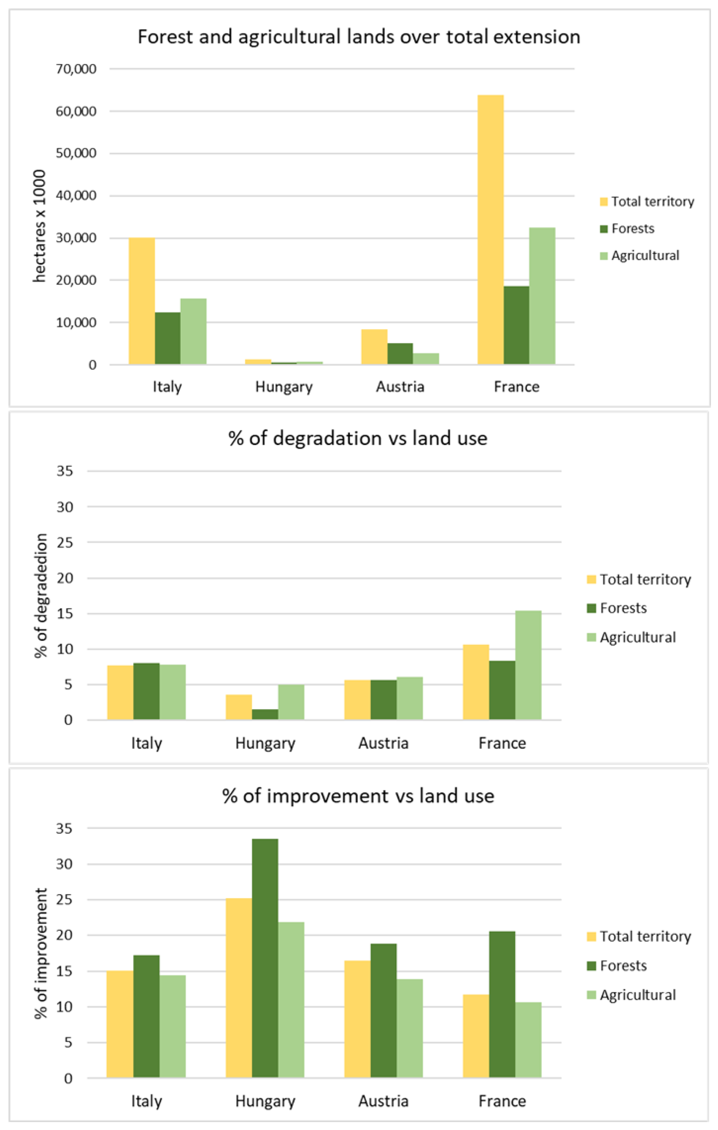
| Land Use Class Extension (ha) | |||
|---|---|---|---|
| Total ROI Extension | Forests | Agricultural | |
| Italy | 30,062,029 | 12,428,000 | 15,642,000 |
| Hungary | 1,342,831 | 489,630 | 746,201 |
| Austria | 8,394,780 | 5,127,264 | 2,678,365 |
| France | 63,848,068 | 18,574,106 | 32,388,971 |
| Degraded (%) | |||
| Italy | 7.67 | 8.03 | 7.78 |
| Hungary | 3.56 | 1.52 | 4.94 |
| Austria | 5.64 | 5.59 | 6.06 |
| France | 10.62 | 8.34 | 15.43 |
| Improved (%) | |||
| Italy | 15.10 | 17.17 | 14.45 |
| Hungary | 25.23 | 33.56 | 21.91 |
| Austria | 16.41 | 18.86 | 13.92 |
| France | 11.70 | 20.61 | 10.58 |
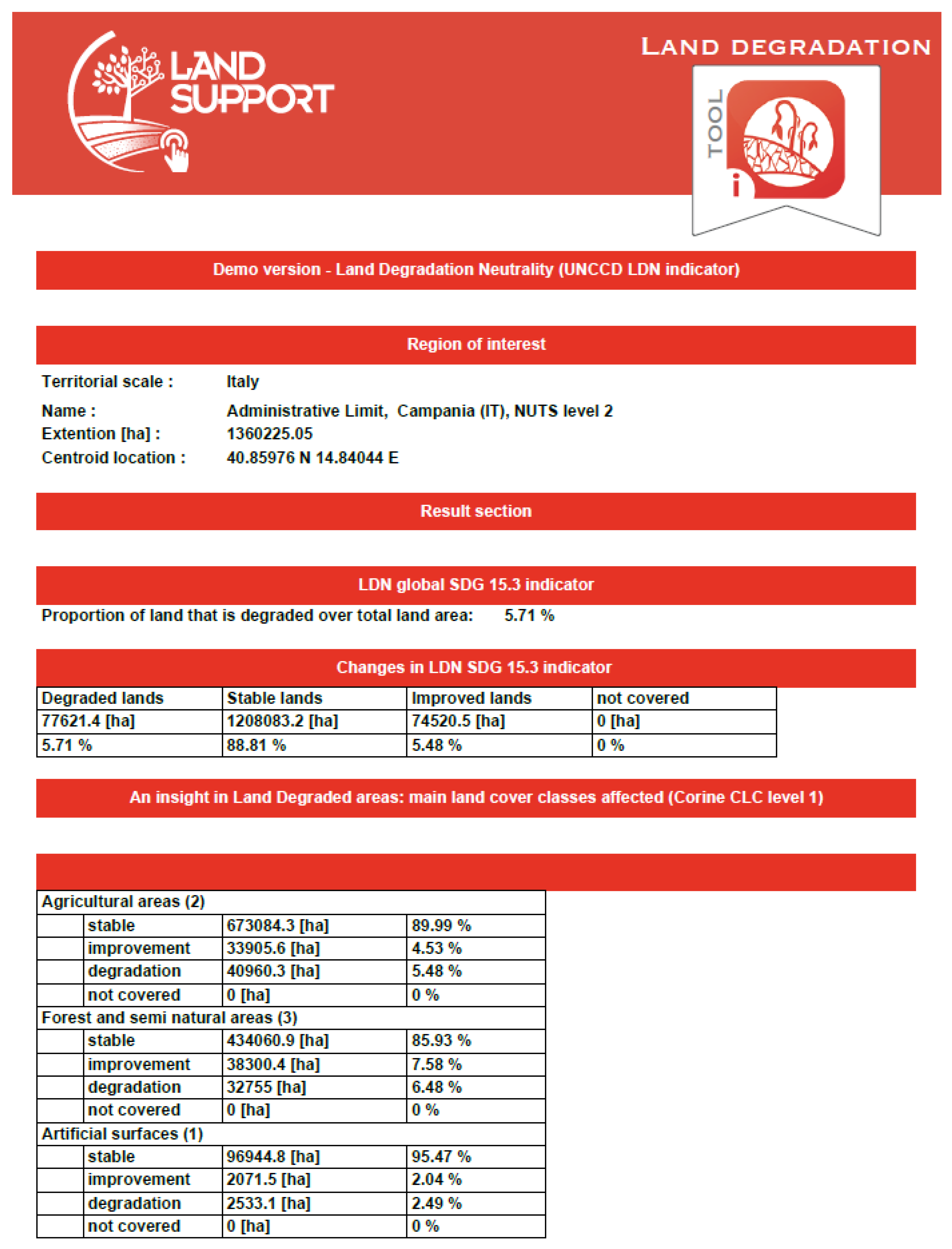
| Indicator Class | Surface Affected (ha) | % Referred to Total ROI Area | Total ROI Area |
|---|---|---|---|
| Degradation | 186.9 | 1.7 | 11,131.2 ha |
| Improvement | 259.1 | 2.3 | |
| Stable | 10,685.2 | 95.9 |
Disclaimer/Publisher’s Note: The statements, opinions and data contained in all publications are solely those of the individual author(s) and contributor(s) and not of MDPI and/or the editor(s). MDPI and/or the editor(s) disclaim responsibility for any injury to people or property resulting from any ideas, methods, instructions or products referred to in the content. |
© 2024 by the authors. Licensee MDPI, Basel, Switzerland. This article is an open access article distributed under the terms and conditions of the Creative Commons Attribution (CC BY) license (https://creativecommons.org/licenses/by/4.0/).
Share and Cite
Manna, P.; Agrillo, A.; Bancheri, M.; Di Leginio, M.; Ferraro, G.; Langella, G.; Mileti, F.A.; Riitano, N.; Munafò, M. A Geospatial Decision Support System for Supporting the Assessment of Land Degradation in Europe. Land 2024, 13, 89. https://doi.org/10.3390/land13010089
Manna P, Agrillo A, Bancheri M, Di Leginio M, Ferraro G, Langella G, Mileti FA, Riitano N, Munafò M. A Geospatial Decision Support System for Supporting the Assessment of Land Degradation in Europe. Land. 2024; 13(1):89. https://doi.org/10.3390/land13010089
Chicago/Turabian StyleManna, Piero, Antonietta Agrillo, Marialaura Bancheri, Marco Di Leginio, Giuliano Ferraro, Giuliano Langella, Florindo Antonio Mileti, Nicola Riitano, and Michele Munafò. 2024. "A Geospatial Decision Support System for Supporting the Assessment of Land Degradation in Europe" Land 13, no. 1: 89. https://doi.org/10.3390/land13010089
APA StyleManna, P., Agrillo, A., Bancheri, M., Di Leginio, M., Ferraro, G., Langella, G., Mileti, F. A., Riitano, N., & Munafò, M. (2024). A Geospatial Decision Support System for Supporting the Assessment of Land Degradation in Europe. Land, 13(1), 89. https://doi.org/10.3390/land13010089