Article

Urban Heat Island and Reduced Habitat Complexity Explain Spider Community Composition by Excluding Large and Heat-Sensitive Species

1
ECOBIO-UMR 6553, CNRS, University of Rennes, F-35042 Rennes, France
2
LTSER ZA Armorique, F-35000 Rennes, France
3
LETG-UMR 6554, CNRS, University of Rennes 2, F-35000 Rennes, France
*
Author to whom correspondence should be addressed.
Land 2024, 13(1), 83; https://doi.org/10.3390/land13010083
Submission received: 14 December 2023 / Revised: 4 January 2024 / Accepted: 9 January 2024 / Published: 11 January 2024

Abstract

:
Along with worldwide urbanization, upheavals in habitat and temperature are major threats for biodiversity. However, due to their interdependence, their relative roles as drivers of animal community composition remain entangled. Here, we investigated how taxonomic and functional compositions of arthropod communities were related to uncorrelated habitat and temperature gradients, and compared landscape (i.e., urbanization, Urban Heat Island (UHI)) to local variables (i.e., vegetation height and cover, near-ground temperature). We sampled 20,499 spiders (137 species) on 36 grasslands in Rennes (northwestern France). Unlike rural areas, urban sites were characterized by short vegetation and intense UHI, hosted species-poor communities, and were composed of small thermophilic species. UHI intensification and local loss of habitat complexity (short and dense vegetation) were associated with declining large and heat-sensitive species. These results highlight the prevalent role of urban warming, rather than land cover change, as an urban filter. Further, we show that landscape-scale UHI, not local temperature, filters species according to their functional attributes. UHI can therefore be considered as a thermal barrier, filtering species according to their physiological capacity to cope with urban thermal conditions. Finally, to counterbalance biotic homogenization, we argue for the importance of implementing complex habitat structures at the local scale within urban green infrastructure.

1. Introduction

The rapid expansion of cities is widely considered to be a major contributor to global biodiversity loss [1]. However, despite an acknowledged global negative impact, the potential of urban areas to conserve biodiversity is often highlighted [2,3]. For instance, urban ecosystems have been shown to support different animal taxa [4], including ground-dwelling arthropods such as carabid beetles and spiders [5]. Whether urbanization supports or disadvantages communities depends on intraspecific and interspecific responses to the new conditions induced by the urban environment [6]. Indeed, urban environments can affect functional trait frequencies and composition, and therefore act as an environmental filter shaping urban community composition according to the ability of species to overcome urban conditions and establish themselves [7,8]. Distinct variables of the urban environment filter have been identified as important drivers of arthropod community composition at local and landscape scales [3,9,10]. These local and landscape variables described in the literature can be grouped in two main categories, habitat and temperature-related variables [11].
With respect to habitat, changes in land cover at the landscape scale were repeatedly identified as important drivers of the loss of arthropod diversity along urbanization gradients [12,13]. For example, parasitoid diversity was significantly negatively affected by the replacement of vegetated areas with impervious surface [14], ground-dwelling beetles with building coverage [15], while ants, beetles, and spiders were related to landscape connectivity variables [16]. In addition to landscape-specific effects, studies also provide evidence of the common role of habitat variables measured at landscape and local scales in explaining the structure of arthropod communities [10,17]. Variables such as the mowing regime or the habitat structural complexity were found to influence arthropod species composition at local scale [5,9].
In addition to habitat conditions, temperature is another widely studied variable. Urban warming has been identified as an important driver of arthropod community composition [18] because arthropods are ectotherms and their metabolism is directly dependent on external temperature [19,20]. At landscape scale, temperatures are strongly influenced by the urban heat island (UHI) phenomenon. The term UHI refers to an increase in the average atmospheric temperature within a city, compared to adjacent rural areas [21]. This phenomenon mainly leads to an increase in night temperatures within urbanized areas [21,22,23]. At local scale, near-ground temperatures also influence arthropod communities [11,24]. However, near-ground temperatures, as experienced by arthropods, can be very different from atmospheric temperatures [25,26,27]. In fact, near-ground temperatures show greater spatial variation than atmospheric UHI and are therefore often referred to as thermal mosaics [24,28]. In urban areas, this is due to the complex interweaving of vegetated and built surfaces [29,30,31]. Considering the temperature recorded at near-ground scale in addition to the UHI in studies of arthropod communities is necessary, as this corresponds to the scale at which arthropods perceive their environment [32]. Consequently, the presence of near-ground thermal variations provides an opportunity to mitigate unfavorable thermal conditions for ground-dwelling arthropods (i.e., behavioral thermoregulation) [33].
Although a few studies have shown direct relationships between atmospheric UHI and arthropod community composition [18,24,34], to our knowledge no study has aimed to link functional trait composition (i.e., the distribution of individual functional traits within a community [35]) to thermal metrics (at both landscape and local scales). Characterizing the links between species’ functional traits and environmental variables would enable us to better understand how species maintain themselves in cities [8], identify species from regional pools that are able to cope with urban environmental conditions, and identify the relevant environmental variables that shape species composition [36]. For example, a landscape habitat variable (i.e., urbanization) was found to shift the functional composition of communities towards more dispersive and thermophilic carabid species [7]. If this study provides fundamental insights into the temperature-induced functional response of arthropods to urban conditions, the actual temperature measurements were not related to functional shifts. Ideally, both near-ground (local) and atmospheric UHI (landscape) temperatures should be recorded. However, this may rarely be possible due to the technical difficulties of implementing comprehensive sensor networks capable of monitoring temperature at different spatial scales.
In ground-dwelling arthropods, several functional traits have been associated with local and landscape environmental conditions. Among them, body size is a key functional trait related to many physiological traits [37] and constrained by environmental conditions. For example, leaf litter depth is positively associated with carabid body size [38,39,40,41]. Reduced grassland management favors the occurrence of both large-bodied carabids and spiders [5,42]. At the landscape scale, urbanization increases the dispersal capacity of spiders [43], while patch isolation favors small, highly mobile carabids [5] and spiders [43]. Finally, body size changes in several arthropods are related to urbanization rate and are thought to be due to temperature increases caused by UHI [44,45]. Hence, UHI-induced warming is generally predicted to drive shifts in ectotherm communities toward smaller species, according to the Atkinson temperature-size rule [46]. The thermal affinity of species is also expected to be an important functional trait driving species community composition at local and landscape scales [7]. If many studies have examined intraspecific changes in critical thermal limits [47,48,49,50,51] and thermal preferences [52] along UHI gradients, almost no studies have considered interspecific thermal traits to test whether changes also occur at the community level. Although a few studies have reported changes in thermal affinities of urban versus rural communities in ants and carabids [7,53], the identification of explanatory variables remains to be investigated. Indeed, our knowledge of functional trait–environment relationships remains scarce with respect to the respective roles of habitat and temperature in explaining arthropod communities. To date, no studies have gone beyond a rural–urban comparison with the aim of disentangling the role of different urbanization-related variables and testing temperature metrics as predictors.
In this study, we used ground-dwelling spiders as a model to assess functional trait–environment relationships along an urbanization gradient. Spiders are ideal biological models because they are abundant, highly diverse, and respond to urban environmental stressors, including landscape and local predictors [5,43,54,55]. Moreover, spiders effectively maintain many ecosystem services by playing important regulatory roles as abundant prey and predators in the food chain [56], notably because of their diversity in terms of functional characteristics, their behavioral or physiological adaptations, but also their evolutionary strategies [57]. Finally, spiders are ectotherms, which makes them particularly sensitive to temperature changes [18]. For example, individuals from warmer locations exhibit higher thermal tolerance [58]. Firstly, we analyzed spider community composition along an urbanization gradient, identified indicator species, and determined which predictor variables drive the abundance of the mainly represented species. Secondly, we characterized the functional traits of spider communities and their relationships with the environment. More precisely, we quantified changes in community-averaged body size, community dispersal capacity, and community thermal affinity in response to urbanization gradient and thermal conditions. Thirdly, we tested whether the observed changes in community functional composition were the result of a functional replacement (i.e., species with particular functional trait scores are discarded while others are favored) or a filtering process (i.e., species with particular trait scores are discarded with little or no replacement).
In order to disentangle the relative effects of habitat and temperature at landscape scale on the functional composition of communities, we selected study sites using a specific procedure that minimizes the covariation between both habitat and temperature variables (see Appendix A for details). To our knowledge, our study is the first to analyze functional trait–environment relationships by simultaneously comparing (1) uncorrelated habitat and temperature variables at landscape scale, (2) local habitat and temperature variables, and (3) temperature variables at landscape and local scales. In line with previous findings on ground-dwelling spiders [45], we expect Atkinson’s rule to prevail [46]. As a result, the size of spiders should decrease in urbanized areas, while dispersal capacity should increase in relation to the rate of urbanization, as densely urbanized landscapes are also more fragmented [59,60]. We can assume that urban communities will be composed of more thermophilic species than rural ones in response to the warmer conditions generated by increased UHI intensity [7,53].

2. Materials and Methods

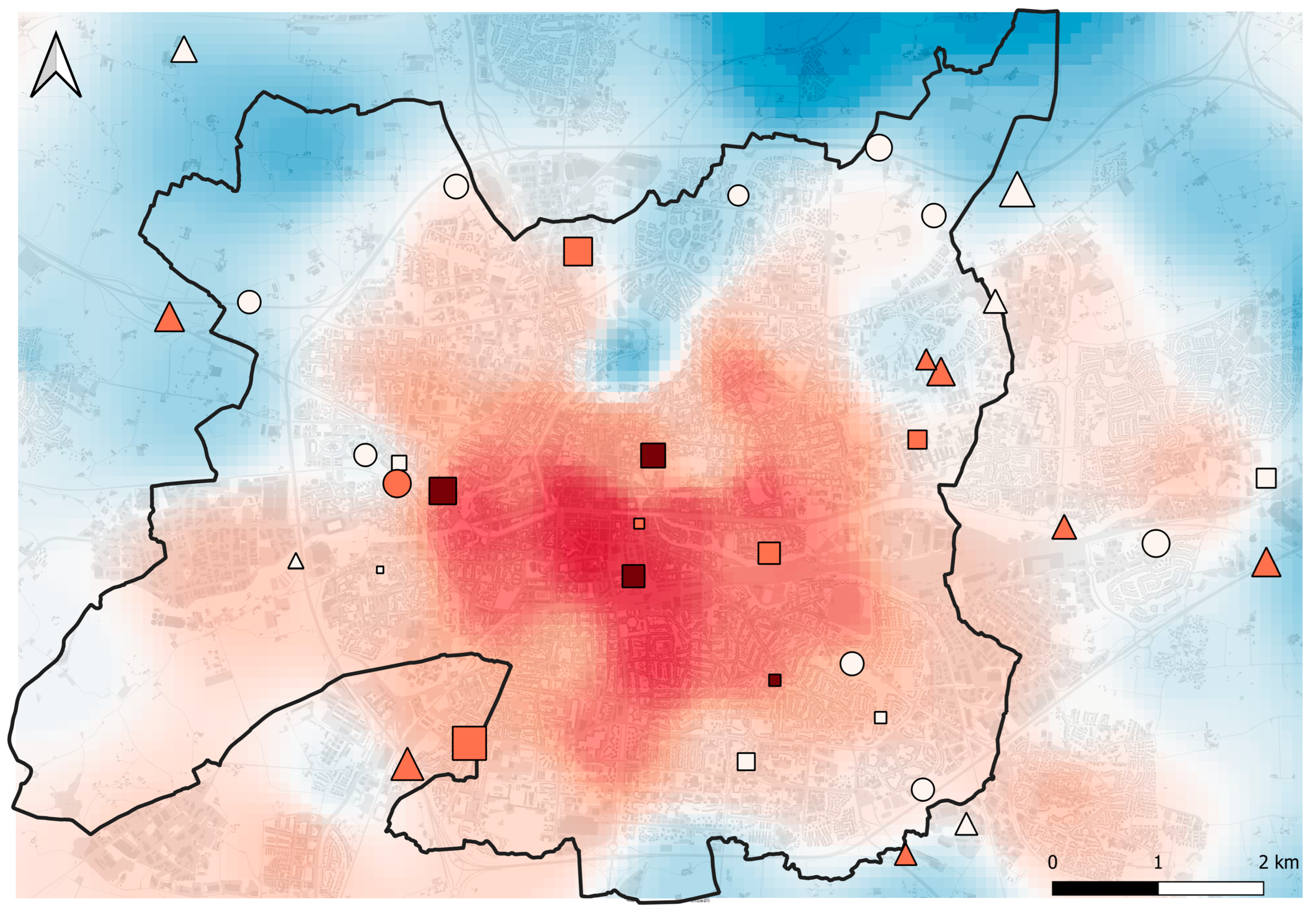
2.1. Study Area and Sampling Sites

This study was conducted in and around Rennes city in the north-west of France (48°06′ N–1°40′ W). Rennes is a city of 227,000 inhabitants. The proximity of the sea (70 km) maintains a temperate oceanic climate. Despite its mild climate, Rennes city faces regular and strong UHI events [23]. We chose grasslands as a model ecosystem because they represent 445 ha (i.e., 56%) of urban green spaces in Rennes [61]. They provide good experimental conditions, as they can support a wide range of vegetation structures, from short and densely seeded lawns in highly managed parks or courtyards to higher and heterogenous vegetation where management is less frequent. Finally, urban grasslands support abundant ground-dwelling arthropod communities [62], ensuring suitable sampling size.
To conduct our experiment, 36 sampling sites were selected on grasslands that had been previously identified as suitable (Figure 1). To select suitable grasslands, we determined areas where urbanization rate and UHI intensity were not highly correlated by performing a spatial correlation analysis based on land cover and UHI maps (see Appendix A for details). The output map allowed us to identify the main decorrelated areas and then select the 36 study sites. The sites were located in public green spaces (N = 10), roadside green spaces (N = 6), communal gardens (N = 12), educational institutions (N = 5), and private gardens (N = 3). Grassland structures ranged from poorly managed meadows to manicured lawns.

2.2. Spider Sampling

Spiders were sampled each month from March to September 2022 using three pitfall traps per sampling site. The three pitfall traps were placed 5 m apart, forming a triangle to ensure capture efficiency [63]. The traps were oriented north, southeast, and southwest. The traps were made of plastic cups (85 mm in diameter and 115 mm in height). We filled them with 150 mL of saline solution at a concentration of 100 g·L−1 to improve spider preservation and a drop of neutral soap to prevent floating. The traps were opened for two weeks each month. After each sampling session, spider individuals were sorted and stored in separate vials containing 70% ethanol. All mature spiders were identified to species level using identification keys [64,65]. Nomenclature followed the World Spider Catalogue version 22 (https://wsc.nmbe.ch/, accessed on 1 December 2022). The dataset used for analysis was obtained by pooling all three traps per sampling site and all seven sampling sessions together.

2.3. Functional Trait Selection

To investigate the functional response of spider communities to their environment, we retrieved information related to body size [64,65,66,67] and dispersal capacity (i.e., ballooning [68,69]) for each species from literature data (Supplementary Materials, Table S1). These traits are known to respond to environmental change along urbanization gradients [5]. Body size influences species physiology, ecological niches, and species’ spatial distribution [45,70]. While sexual dimorphism is common in spiders, we retrieved only the body size of females [45]. Dispersal capacity informs on species ability to escape their home range to avoid competition or adverse environmental conditions [71].
We also estimated the thermal niche of species to test whether urban environmental conditions filter species according to their thermal affinities. We followed a method described in the literature [7,72] to assign temperature attributes to species according to their spatial distribution in Europe and North Africa. Accordingly, we extracted species distribution information for all recorded species from the online database Spiders of Europe [67] and we retrieved gridded European mean, maximum, and minimum daily temperatures between 2011 and 2022 [73]. From the temperature data, we extracted the averaged mean, maximum, and minimum temperature per country. The average temperatures of countries where a species is present were then used to calculate the thermal niches of the species, resulting in three thermal affinity values per species: mean, maximum, and minimum thermal affinity.

2.4. Environmental Variables

To characterize habitat and temperature variables, we collected two and three environmental variables at landscape and local scales, respectively (see Table 1 for details). Variables measured at landscape scale were the proportion of impervious surface (a commonly used proxy for urbanization) [74] and the mean UHI intensity calculated over the entire study period as a proxy for urban atmospheric warming [23,52]. To calculate these two landscape variables, we chose 100 m as the radius size of the circular buffers around the sampling sites. This buffer size has been found to cover an adequate area to provide landscape-scale information related to the urban matrix that drives arthropod communities [17,75]. Furthermore, it corresponds to the finest spatial resolution of atmospheric UHI data available in our study area and it matches the scale at which the correlation between urban land cover (i.e., built-up area) and atmospheric UHI remains lowest in Rennes [22]. We did not include any additional landscape variables related to vegetation cover, since urbanization and vegetation (including wooded areas) were strongly negatively correlated (r = −0.8).
At the local (i.e., site) scale, we characterized vegetation structure by measuring the percentage of vegetation cover and the height of the vegetation. These predictors are regularly used to characterize the habitat of arthropod species [15]. In addition, we monitored the air temperature just above the surface (i.e., 5 cm) during the study period to obtain a record of the near-ground temperature experienced by the spiders (see Table 1 for details).

2.5. Data Analyses

2.5.1. Characterization of the Urbanization Gradient

To establish a typology of sites according to their contrasts in environmental characteristics, we performed a hierarchical clustering analysis (HCA) based on all scaled environmental variables. We used the ‘HCPC’ function and the ‘Ward’ method to construct the tree in the ‘FactoMineR’ package (version 2.7) [76]. The optimal number of clusters was determined according to the partition with the higher relative loss of inertia [76]. Once the sites were grouped into clusters, we performed a silhouette analysis to check the agreement of individual sites with their own cluster, using the ‘silhouette’ function from the ‘cluster’ package (version 2.1.4) [77].

2.5.2. Spider Community Composition along an Urbanization Gradient

The composition of spider communities across environmental clusters obtained by HCA was analyzed using non-metric multidimensional scaling (NMDS, Bray–Curtis dissimilarity) with the ‘vegan’ package (version 2.6-4) [78]. For ordination, species abundances were square root transformed. We then tested whether communities differed significantly between clusters by performing a pairwise permutational multivariate analysis of variance (9999 permutations) using the ‘pairwise.perm.manova’ function from the ‘RVAideMemoire’ package (version 0.9-83-3) [79]. Finally, all environmental variables were fitted in ordination space and their significance was tested using a Monte Carlo randomization procedure (9999 permutations).
Indicator species were assessed using the fidelity and exclusivity of species to the resulting clusters of sites using the IndVal (indicator value) procedure in the ‘labdsv’ package (version 2.0-1) [80]. Indicator values were calculated from the species abundance matrix, taking into account both relative abundances and frequencies of occurrence within each individual cluster. Significance of indicator values was tested at a p-value < 0.05 using a Monte Carlo randomization procedure (9999 permutations). Species with both an indicator value > 0.5 and a significant p-value were considered to be accurate indicators.
To test the response of the 29 most represented species (including indicator species) to environmental variables, we fitted Poisson generalized linear models (GLMs). Since overdispersion was detected, we corrected standard errors by using a quasi-Poisson GLM [81]. We assessed the goodness of fit by calculating the adjusted R2, with the ‘rsq’ function from the ‘rsq’ package (version 2.5) [82]. To reduce statistical noise, all observations comprising fewer than three individuals per site and per sampling period were removed from the dataset used to perform statistical analysis on community composition and indicator species.

2.5.3. Relationships between Functional Traits and Environmental Conditions

For each trait (i.e., body size, ballooning, and thermal affinity), we obtained a trait community index by calculating community-averaged trait scores. As a binary trait, ballooning was considered as numerical, and a community-averaged value between 0 and 1 was calculated. In order to account for the functional attributes of rare species in the calculation of community-averaged indexes, we considered all species and did not weight the community-averaged traits by species abundance. To test whether significant differences in trait community indices existed between clusters, we performed a one-way ANOVA using the ‘aov’ function, followed by a post-hoc Tukey test using the ‘Tukey-HSD’ function. To identify the direction of variations of each trait, we built a GLM with each community-averaged trait score as the response variable and all five environmental variables as predictors. For all models, we assumed a normal distribution and assessed goodness of fit by the adjusted R2 calculated using the ‘rsq’ package (version 2.5) [82].

2.5.4. Characterization of Changes in Functional Trait Community Indices

Finally, we analyzed whether changes in functional trait community indices were the result of replacement by species with particular trait scores within communities, or whether they were due to a decline in certain species (i.e., species filtering). To achieve this, we categorized species according to their continuous functional trait scores [7] (i.e., body size and thermal affinity). To define species categories, cutoff functional trait scores were chosen to yield three groups with balanced numbers. Species are thus divided into small, medium, and large species with respect to body size, or into low, medium, or high according to their affinity to temperature with respect to thermal niche. We used one-way ANOVA followed by a post-hoc Tukey test to determine whether species with particular functional trait categories were over- or under-represented in the cluster communities in terms of absolute and relative species richness. We also tested whether specific environmental variables were associated with increases or decreases in the richness of species with specific functional trait using the same GLM as described above, but with absolute species richness as the response variable.
All statistical analyses were performed in R version 4.2.2.

3. Results

3.1. Sampling Results and Urbanization Gradient

A total of 20,499 adult spiders were captured, belonging to 21 families and 137 species. The most represented families were Linyphiidae (N = 8807; 43%), Lycosidae (N = 4951; 24.2%), and Tetragnathidae (N = 5023; 24.5%). The most abundant species were Pachygnatha degeeri (N = 4913; 24%) and Pardosa cf. tenuipes (N = 2490; 12%).
The hierarchical classification of sampling sites led to the identification of three distinct clusters characterized by contrasted environmental conditions (Figure 2). The first cluster (‘high vegetated rural’) includes sites with both low UHI intensity and urbanization at the landscape scale, while at the local scale the herbaceous vegetation was high, dense with low near-ground temperatures. The second cluster (‘short vegetated rural’) includes sites with both low UHI intensity and urbanization, while at the local scale, the vegetation was short, sparse, with intermediate near-ground temperatures. The third cluster (‘short vegetated urban’) includes sites with both high UHI intensity and urbanization, while at the local scale, the vegetation was short, sparse, with high near-ground temperatures.

3.2. Spider Community Composition and Indicator Species along an Urbanization Gradient

Excluding species with fewer than three occurrences per site and per sampling session resulted in 20,049 adult spiders (i.e., 98% from total abundance) belonging to 85 species (62% from total species richness) subjected to NMDS ordination (Figure 3). The final stress value of 0.17 indicates a good representation of the community distribution by the scaling. Spider communities from both rural clusters (i.e., ‘high vegetated rural’ and ‘short vegetated rural’) did not significantly differ among each other (p = 0.81), but were significantly different from communities belonging to the ‘short vegetated urban’ cluster (p = 0.002, respectively). Examination of individual environmental variables revealed that spider communities were significantly structured by UHI intensity (p < 0.001), urbanization (p = 0.004), near-ground temperature (p < 0.001), and vegetation height (p = 0.002).
Although the composition of communities differed significantly between clusters, several dominant species were shared by the three clusters. For example, P. degeeri, P. cf. tenuipes or Tenuiphantes tenuis were abundant in the three clusters (Table 2). We identified six indicator species in total, three for ‘high vegetated rural’ sites and three for ‘short vegetated urban’ sites.
The GLM analysis of the abundances of the 29 most abundant species revealed that UHI and near-ground temperature were each associated with seven species (Table 3), representing 24.21% and 41.09% of the individual count, respectively. Near-ground temperature was negatively related to abundance, whereas UHI was associated to contrasted responses. For instance, Erigone dentipalpis indicated ‘short vegetated urban’ sites and was positively related to UHI. In contrast, Pardosa pullata indicated ‘high vegetated rural’ sites (Table 2) and was less abundant when UHI and near-ground temperature increased (Table 3). Similarly, indicators of ‘short vegetated urban’ sites became rarer with increasing vegetation height (Table 3), whereas P. pullata was supported.

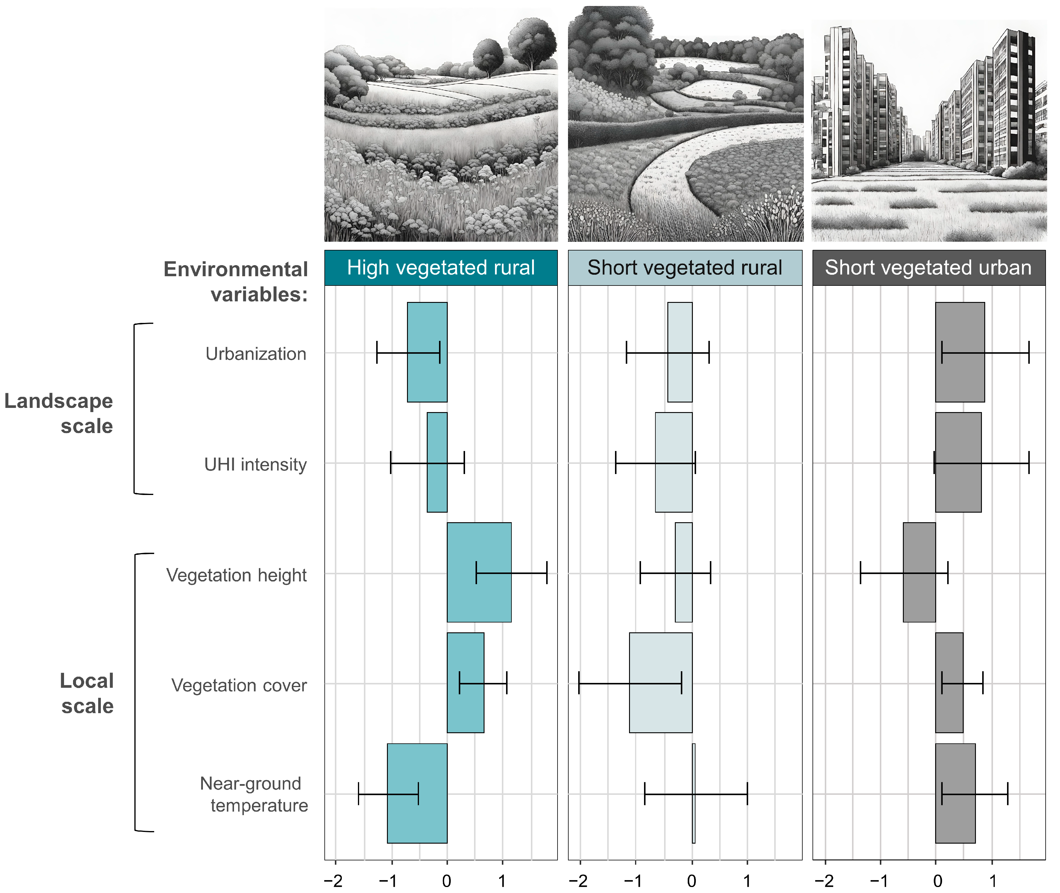
3.3. Relationships between Functional Traits and Environmental Conditions

Mean community body size varied significantly between clusters (Figure 4, p = 0.04). The mean community size of spiders was significantly lower (4.00 mm) in high vegetated urban sites, compared to short and high vegetated rural sites (4.34 mm and 4.58 mm, respectively). GLM analysis showed that body size was positively related to vegetation height (coeff. = 0.28, p = 0.02, adjusted R2 = 0.21). Community ballooning capacity did not differ significantly between clusters (p = 0.50). GLM analysis showed a significant negative relationship between community ballooning capacity and vegetation height (coeff. = −0.03, p = 0.02, adjusted R2 = 0.16).
We found significant differences in community thermal affinities between ‘high vegetated rural’ and urban sites (Figure 5). Urban sites systematically had higher community thermal affinities with mean affinities of 10.30 °C (mean thermal affinity), 15.10 °C (maximum thermal affinity), and 5.80 °C (minimum thermal affinity), whereas high vegetated rural sites had lower values with 10.10 °C (mean thermal affinity), 14.90 °C (maximum thermal affinity), and 5.60 °C (minimum thermal affinity). No relationship with environmental variables was identified by GLM analysis regarding the thermal affinity. As the changes in the community-averaged thermal affinity were similar whether the index was calculated from mean, maximum, or minimum temperatures, only the mean community thermal affinity is considered in the following results and discussion.

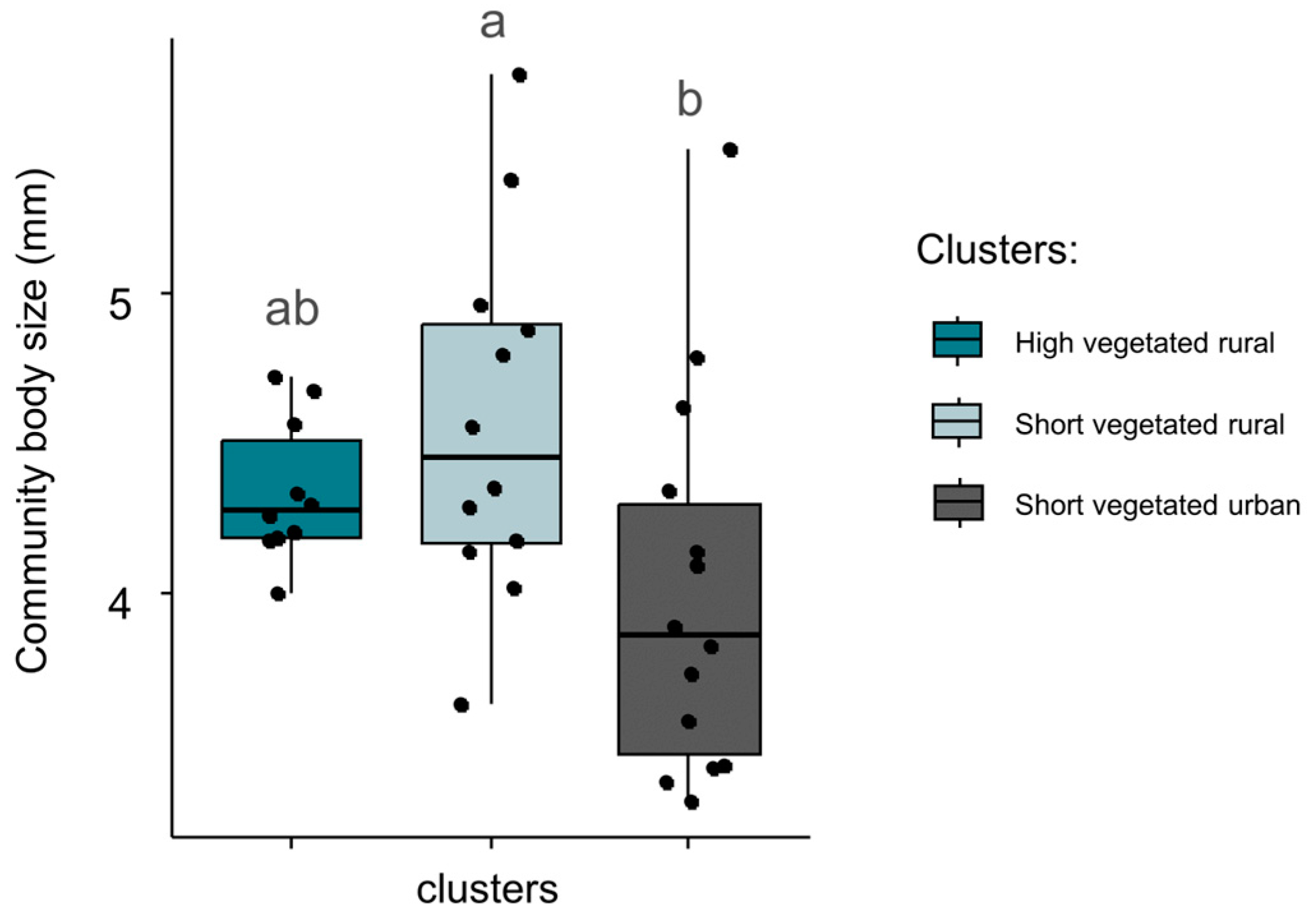
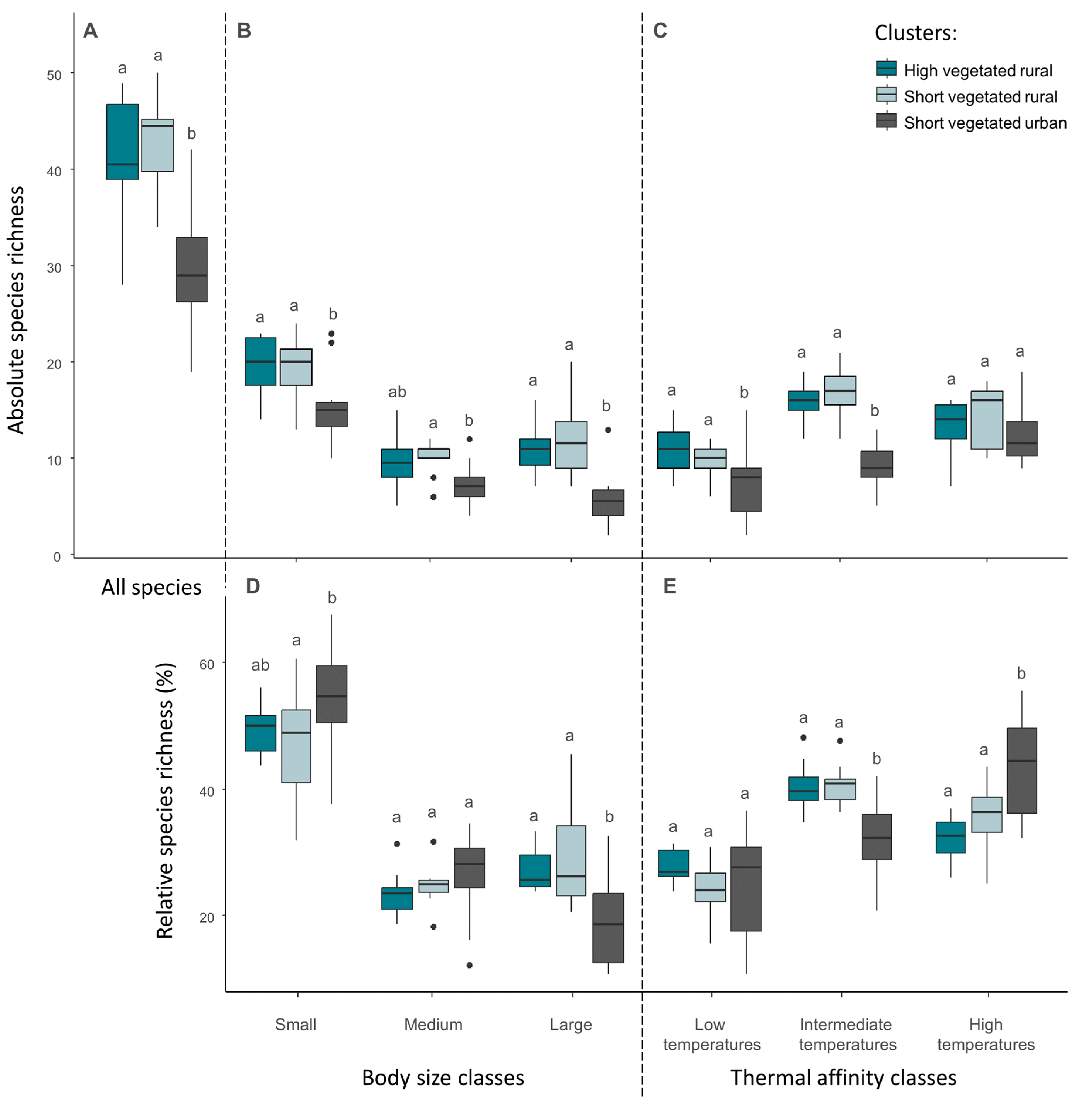
3.4. Characterization of Changes in Functional Trait Community Indices

The total number of species was significantly lower in the ‘short vegetated urban’ cluster, compared to ‘high vegetated rural’ and ‘short vegetated rural’ (Figure 6A). Among species classes sorted by body size, the number of small and large species was significantly lower in the urban cluster compared to both rural ones, whereas the number of medium species differed only between the urban cluster and the ‘high vegetated rural’ (Figure 6B). Proportionally, small species increased whereas large species decreased in the urban cluster, compared to both rural ones (Figure 6D). We observed a decrease in the absolute number of species associated to low and intermediate temperatures in the urban cluster, compared to both rural ones (Figure 6C). In the case of species related to high temperatures, the number of species did not differ between clusters. The decreasing absolute species richness in species associated to low and intermediate temperatures resulted in an increased proportion of species associated to high temperatures in the urban cluster, compared to the rural ones (Figure 6E).
Analysis of the effect of environmental variables on variation in absolute species richness showed that the variables studied had a strong influence on large species (Table 4). In particular, UHI intensity is negatively related to the number of large species, whereas the vegetation height is positively related to the number of large species. In addition, the number of species related to low and intermediate temperatures were negatively related to UHI intensity, whereas the number of species related to intermediate temperatures was also explained by vegetation attributes (Table 4).

4. Discussion

4.1. Spider Community Composition and Indicator Species along an Urbanization Gradient

We showed that spider community composition varies between urban grasslands, depending on their environmental characteristics. Urbanization rate, UHI intensity, near-ground temperature, and vegetation height were identified as factors dissociating the three clusters of sites with contrasting environmental conditions. While some species are shared with similar abundance across the three clusters (e.g., P. degeeri, P. cf. tenuipes, T. tenuis), we found that species composition contrasted strongly in terms of occurrence and abundance between clusters (Table 2). In particular, we found that ‘high vegetated rural’ and ‘short vegetated urban’ clusters present indicator species.
In high vegetated rural sites, the two wolf spider species identified as indicators are closely related species (i.e., Pardosa prativaga and P. pullata). They are known to commonly co-occur in a widely overlapping range of vegetation structures, although some differences in habitat preference have been observed, particularly in case of interspecific competition [83]. Both species are typical of herbaceous vegetation (i.e., agricultural meadows), although P. pullata prefers open microhabitats with low vegetation, whereas P. prativaga prefers denser and higher vegetation [83]. Our results show that near-ground temperature is the variable mostly related to the abundance of P. pullata across the 36 study sites. Therefore, this result suggests that the stronger association of P. pullata with high-vegetated grasslands (i.e., meadows) than with short-vegetated grasslands (i.e., lawns) may not be determined by a particular habitat structure, but could rather result mainly from locally adapted temperature conditions. We identified two common and widespread linyphiid spiders, Erigone atra and E. dentipalpis, as indicator species associated with urban sites characterized by intense UHI conditions, short and dense vegetation, and high near-ground temperatures. These two species are phylogenetically close and co-occur frequently. They share identical life cycles, niches, and habits [84,85]. Both species have been well studied in agricultural landscapes and previous studies have reported high dispersal capacities (i.e., by ballooning) as well as a particular ability to colonize new habitats in a short time after human-induced disturbance. In the light of our results, these conclusions drawn from the agricultural context can easily be transposed to the urban environment. If agricultural fields are regularly disturbed by multiple operations throughout the year, urban grasslands may also be subject to multiple mowing operations. The fact that E. atra and E. dentipalpis are indicators of short vegetated grasslands found in urban areas is therefore not surprising, since these are also the most frequently mown. In addition, Cryptachea blattea was indicator for urban areas. This species was first described in New Zealand and is spreading rapidly throughout Europe, as evidenced by the first records made in the last decade in several European countries (Germany in 2008 [86], Britain in 2011 [87], Switzerland in 2013–2014 [88], France in 2014 [89], the Netherlands in 2014 [90], and Ireland in 2019 [91]). The majority of these new records were made in anthropogenic environments, such as ornamental gardens or nurseries [91]. The strong positive relationship observed between C. blattea abundance and the urbanization rate is therefore in line with previous studies. It indicates that the presence of C. blattea is probably related to the intensive use of horticultural plants, which are widely planted in cities’ urban parks and green infrastructures. The absence of indicator species associated with the ‘short vegetated rural’ cluster may be explained by heterogeneous environmental characteristics of sites [92].

4.2. Relationships between Functional Traits and Environmental Conditions

As a first step, to determine whether the spider communities belonging to the three identified clusters were functionally distinct, we tested whether the community-averaged body size differed between clusters. We observed a significant decrease in body size in urban spider communities associated with the highest levels of urbanization, UHI intensity, and near-ground temperature (Figure 7). This result is consistent with previous research showing that community-averaged body size of terrestrial arthropods generally tends to decrease with increasing urbanization [93,94,95]. Furthermore, this relationship has recently been linked to temperature increases in urban areas caused by the UHI effect [45]. However, our examination of the links between body size and environmental variables (taken individually) calls this latter hypothesis into question. It revealed that vegetation structure (more that the UHI) was related to changes in community-averaged body size. Interestingly, community-averaged dispersal capacity was also related to local vegetation attributes, although no differences among clusters were observed. This is consistent with previous studies, showing a lack of relationship between landscape-scale urbanization rate and community-averaged dispersal capacity of spiders [5]. It is therefore not surprising that the community-averaged functional traits (i.e., body size and dispersal capacity) showed significant relationships with the vegetation height. The fact that short-vegetated habitats, whether in rural or urban areas, host smaller, more dispersive species than high-vegetated habitats is supported by previous findings concerning spiders. Indeed, community-averaged body size is driven by local vegetation height [42]. In addition, a decrease in vegetation structure complexity may prevent colonization and establishment of large prey, which in turn may limit feeding opportunities for large spiders. Although we focus on the community-averaged body size response, intraspecific changes in functional trait can occur along urban environmental gradients, resulting either from phenotypic plasticity or genetic adaptation [96]. For example, moths showed that intraspecific body size changes toward smaller individuals with increasing temperature. It is consistent with the observed global trend observed at the community level, characterized by a negative relationship [44]. In spiders, however, only a few species have been the subject of such studies (e.g., [97]). Future urban studies on spiders should compare the intraspecific variation in body size across species. This approach would enable researchers to determine whether community-averaged and intraspecific changes are consistent, or whether the direction of relationships with environmental drivers is species-dependent [44].
In a second step, we tested whether changes in community-averaged thermal affinity occurred between clusters. We observed a significant increase in thermal affinity in the urban cluster, compared to communities in the ‘high vegetated rural’ cluster. This suggests that thermophilic species are favored by urban environments (Figure 7). Similar community-averaged functional changes along an urbanization gradient have been observed in ants [53] and grassland carabid communities [7]. In these studies, changes were interpreted as a result of species being selected to succeed in intense UHI conditions thanks to an affinity for high temperatures (which diverges from our UHI index based on daily minimum temperatures). Species tolerating a wider range of temperatures were hypothesized to be favored in urban areas [7]. These authors found only the thermal affinity index based on maximum temperatures to increase with urbanization, while the index based on minimum temperatures did not respond. This latter assumption is contradicted by our results, since we observed a constant change, whether the mean, minimum, or maximum temperature index was considered. If the range of temperature tolerance does not change in our study system, interspecific variation in critical thermal limits (i.e., CTmax) may be of prime importance. For example, in a study exploring the relationship between thermal tolerance of bee species and their ability to persist under intense UHI conditions, thermal tolerance was shown to be a critical thermal trait for predicting species-specific responses to warming [98]. This study highlights the importance of species’ thermal physiology in shaping community compositions through functional filtering processes. This importance is also supported by the large number of studies focusing on intraspecific variation in thermal tolerance [47,48,49,50,51]. An alternative explanation for the observed change in community-averaged thermal affinities could be an indirect effect of body size, through the covariation of species’ thermal affinity and body size. Intraspecific studies on spiders have already shown that larger individuals tend to prefer higher temperatures [52], and the general positive association between body size and thermal tolerance is striking in arthropods [99,100,101]. However, as we found that species’ trait for body size and mean thermal affinity are weakly correlated (r = 0.22), we argue that the predominant patterns from intraspecific studies cannot be extended to the community level in our system. Furthermore, communities sampled in warm urban sites, and therefore belonging to the urban cluster, were composed of smaller species than rural communities, which in itself invalidates this alternative interpretation. Nevertheless, it cannot be excluded that traits other than thermal affinity are associated with biogeographical distribution and directly or indirectly influence the ability of species to succeed in urban areas.

4.3. Changes in Functional Trait Community Indices

Finally, we aimed to investigate the mechanisms associated with the observed changes in community-averaged functional traits, by assessing the role of functional replacement versus filtering between environmental clusters. We found that sites belonging to the urban cluster were less rich in species than sites belonging to the two rural clusters. This confirms previous results obtained on carabids, supporting the filtering process theory [7]. Under this condition, community-averaged functional changes result, at least partially, from a subset of species with particular trait values, enabling them to establish in urban environmental conditions [7,102]. We further aimed to understand the mechanisms underlying the observed community-averaged functional changes by studying the variations in species richness partitioned into classes of species characterized by particular functional trait values.
We found that urban sites were linked to a decrease in species richness in all body size classes (e.g., small, medium, large). This decrease in species number was more important in large species than in small and medium species. Therefore, the decrease in community-averaged body size in urban sites results from a size-related loss of species, with the urban filter being more effective for larger species. Furthermore, this acute loss of large species within urban spider communities could be the direct result of a negative effect of temperature increase. Indeed, the number of large species was strongly negatively related to the UHI intensity. This result is in line with the global prediction of a warming-induced decrease in body-size within communities of ectothermic taxa [103]. At the scale of a city, UHI could limit the body size of spider communities by increased metabolic costs in warmer conditions compared to adjacent rural areas, allowing only small and medium-sized species to maintain themselves. Such filtering of large species reflects common temperature-size rules observed at the intraspecific level. For example, Bergmann’s rule states that warmer conditions (e.g., low latitudes or altitudes) are associated with intraspecific changes in body size in favor of smaller individuals [104]. Furthermore, according to Atkinson’s rule, ectothermic individuals that have developed in warm conditions generally become smaller in the adult stage than individuals from colder environments [46]. Furthermore, our analysis of species richness confirms the importance of local vegetation structure as a driver of the community-averaged body size. It also indicates that these variables are particularly determinant of the presence of large species. In the light of our results, the loss of availability of vertical and horizontal structural complexity of the vegetation through decreasing height and increasing density limits the establishment of large species. This suggests that vegetation homogenization, e.g., by increasing mowing frequency, limits the establishment of large spiders, possibly by reducing hiding opportunities or the availability of large prey [42].
The hypothesis of a functional filtering process is also supported by an examination of species richness distribution within thermal affinity classes. Indeed, we found that the increase in community-averaged thermal affinity in the urban cluster resulted from an increased proportion of thermophilic species, combined with a reduced proportion of species associated with intermediate temperatures. Closer examination of the absolute number of species reveals that these changes in proportions are due to a relatively greater deficit of species with low and intermediate temperature affinities in the urban compared to the rural clusters. As with body size, the difference in community-averaged thermal affinity observed between urban and rural clusters is therefore the result of decreasing species richness when comparing the rural clusters to the urban one. It indicates a functional filtering process. Indeed, the absence of an absolute increase in thermophilic species in sites belonging to the urban cluster shows that the observed functional trait change toward higher temperature values is due to a filtering process against heat-sensitive species in urbanized areas. Detailed analysis of individual variables showed that this functional filtering is linked to the intensification of UHI conditions. This result provides a better understanding of the mechanisms. Indeed, previous studies have linked changes in community-averaged temperature affinities to global urbanization but have not formally identified the underlying driving variables. Our study provides the first evidence that temperature is the determining variable and goes further by showing that landscape-scale UHI, rather than local temperature increase, filters species according to their thermal affinities. Thus, the large heat zones generated by the UHI effect can be considered as thermal barriers at the edge of the city, where only species physiologically able to cope with urban warming persist. On the contrary, near-ground temperature in cities has been shown to be a dominant factor associated with the abundance of locally present species, as supported by previous studies on different arthropod groups [24,105,106].

5. Conclusions

Our study shows that changes in the functional composition of spider communities occurs at both local and landscape scales and those functional traits are filtered at both scales. Landscape-scale UHI negatively affects species richness by filtering species according to their thermal affinity, leading to biotic homogenization at the community level. Furthermore, the local habitat structure is also related to the functional composition of spider communities. Indeed, the reduction in vegetation height led to a reduction in the number of species, with larger species being extirpated. As the vegetation in urban sites was on average shorter than in rural sites in our study system, urban communities changed towards low-diversity communities composed of small species. As predatory arthropods, spiders play an important role in the trophic chain, controlling a wide range of invertebrates. Consequently, lower abundance of specific functional traits due to reduced species richness may lead to imbalance in urban ecosystems caused by a lack of biocontrol at lower trophic levels. Here, we provide further evidence that complexifying grassland vegetation, e.g., by increasing mowing height or decreasing management frequency, enables the establishment of more functionally diverse communities. Improving the structure of green infrastructures could therefore not only compensate for the loss of species induced by urban warming at taxonomic and functional levels, but also help to locally mitigate the effects of the UHI [107], thus offering valuable co-benefits to urban climate and biodiversity.

Supplementary Materials

The following supporting information can be downloaded at: https://www.mdpi.com/article/10.3390/land13010083/s1. Table S1: Species list of spiders and related traits based on literature data [64,65,66,67,68,69].

Author Contributions

B.B., H.Q. and V.C. conceived and designed the study. V.D. and V.C. conducted the field work and analyzed the data. V.C. wrote the first draft of the manuscript. B.B., H.Q., V.D. and A.R. contributed substantially to revisions. All authors have read and agreed to the published version of the manuscript.

Funding

This project received financial support from the region of Brittany for financing this research as part of the ARED program. This project received financial support from the CNRS through the MITI interdisciplinary programs through its exploratory research program (project “BiodivR”).

Data Availability Statement

Data is contained within the article.

Acknowledgments

We thank the team of the Department of Plant Ecology from the Technische Universität Berlin for having made temperature loggers available to us during the time of the experiment. We also thank Rennes Métropole, the DJB (Direction des Jardins et de la Biodiversité) of Rennes, the city councils of Cesson-Sévigné, Chantepie, Saint-Jacques-de-la-Lande, the high school Emile Zola, the Institut Agro Rennes, the DIR Ouest, and all community gardens for having authorized and helped us with the sampling.

Conflicts of Interest

The authors declare no conflicts of interest.

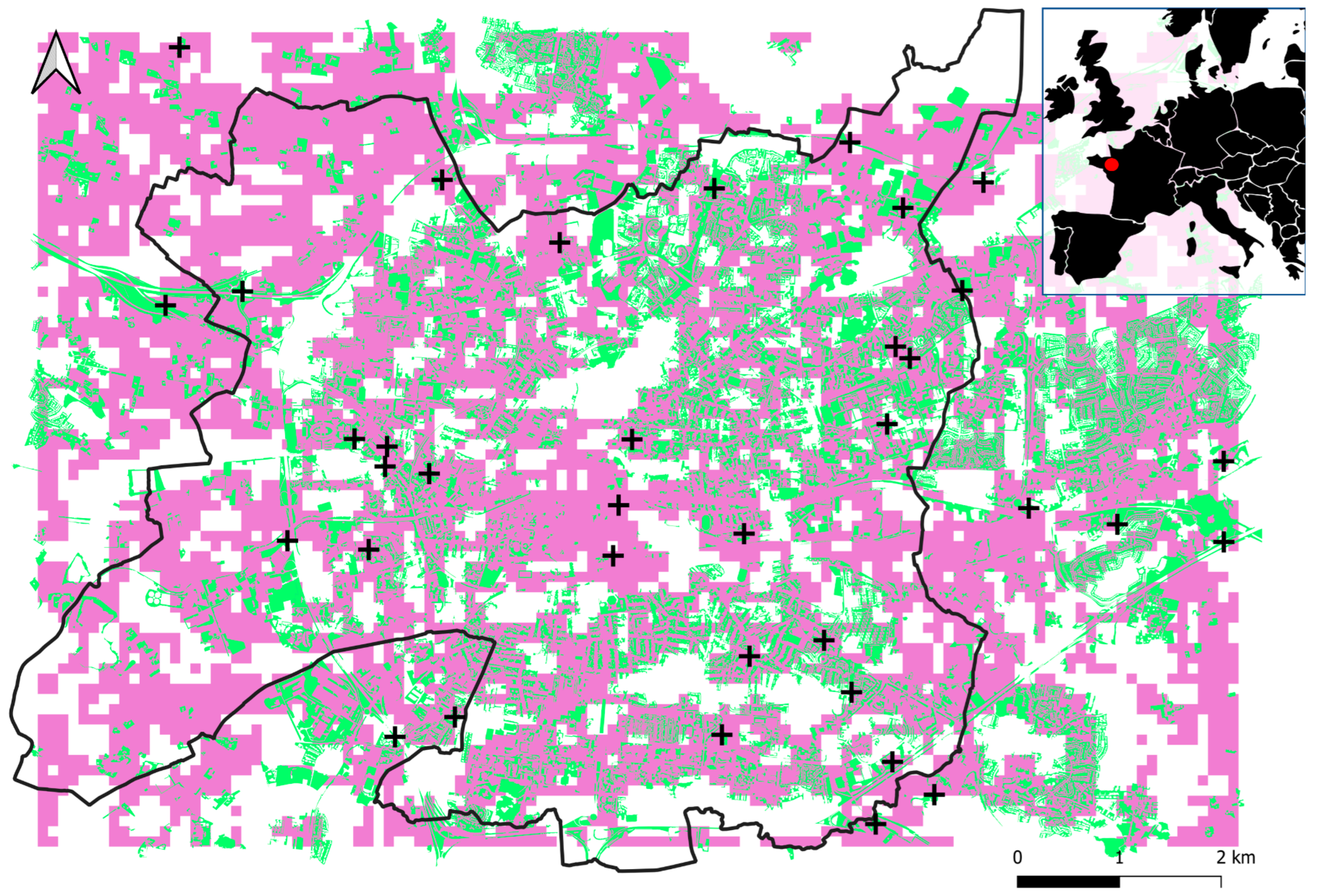
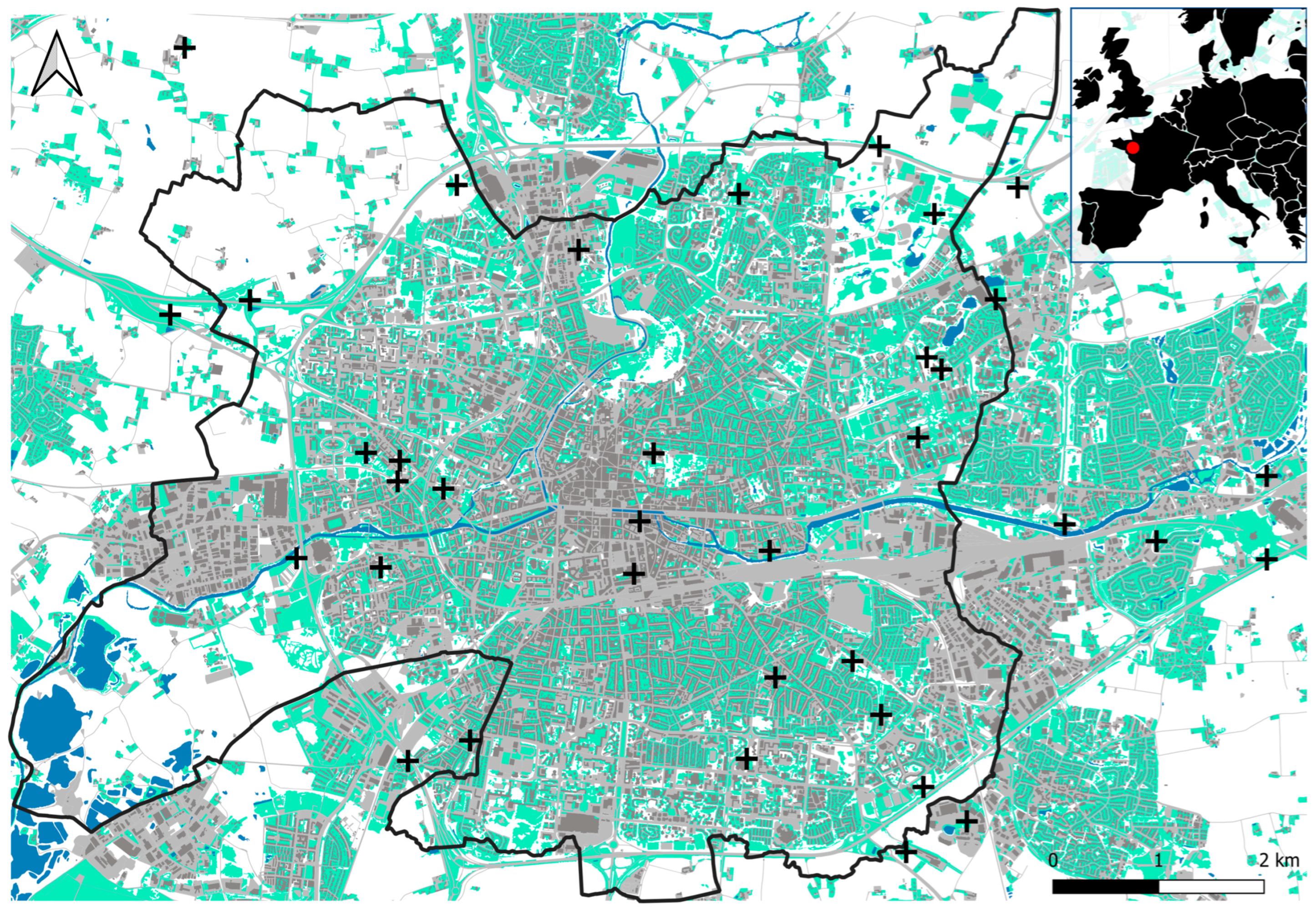
Appendix A. Sampling Site Selection Procedure

Prior to data collection, we performed a spatial analysis in order to identify suitable sampling areas where land cover and atmospheric UHI were not significantly correlated. We based this sampling site selection procedure on two maps: a raster map showing the proportions of built-up areas and a raster map showing the intensity of the atmospheric UHI in 2020 (both at 100 m resolution). As the proportion of built-up areas was identified as a major factor in atmospheric UHI intensity in Rennes [22], we identified the areas where the two maps were least spatially correlated. To achieve this, we proceeded as follows:
(1)
We performed a Spearman spatial correlation analysis to identify all pixels showing a non-significant covariation between atmospheric UHI intensity and the proportion of built-up areas. This analysis was performed using the ‘rasterCorrelation’ function from the ‘spatialEco’ package (version 1.3.7). Correlations were calculated within a 500 m square sliding window (i.e., 25 pixels), centered on each map pixel. This window size corresponds to a trade-off between a number of pixels large enough to calculate a reliable correlation (N = 25) and an area small enough (25 ha) to identify uncorrelated areas;
(2)
We extracted all pixels corresponding to non-significant correlations (p-value > 0.05), resulting in a raster map indicating suitable (i.e., uncorrelated) areas for sampling;
(3)
We selected all patches of herbaceous vegetation (excluding agricultural fields) from the Rennes land cover map that overlapped the suitable sampling area (Figure A1);
(4)
We identified 39 accessible sampling sites encompassing a broad gradient of built-up cover proportions and UHI intensities;
(5)
Once fieldwork was completed in 2022, we repeated the first four steps with updated atmospheric UHI data from 2022 corresponding to the arthropod sampling period, to check that all sampling sites were still located in suitable (i.e., uncorrelated) areas;
(6)
We removed three sites located in unsuitable areas, resulting in 36 remaining sampling sites.
This sampling site selection procedure was an important prerequisite, as it determined the subsequent discrimination of individual effects of land cover (i.e., urbanization) and atmospheric UHI related to arthropod communities.
Figure A1. Map of Rennes (black line) and its surroundings. Areas identified as suitable for sampling (uncorrelated) after spatial correlation analysis are in purple (p-value > 0.05) and associated intersecting grasslands are in green. Impervious surface is displayed in grey. Black crosses display sampling sites. The red dot on the map at top right indicates the location of the study area.
Land 13 00083 g0a1

References

  1. Elmqvist, T.; Fragkias, M.; Goodness, J.; Güneralp, B.; Marcotullio, P.J.; McDonald, R.I.; Parnell, S.; Schewenius, M.; Sendstad, M.; Seto, K.C. Urbanization, Biodiversity and Ecosystem Services: Challenges and Opportunities: A global Assessment; Springer Nature: Berlin/Heidelberg, Germany, 2013; ISBN 978-94-007-7087-4. [Google Scholar]
  2. Shwartz, A.; Turbé, A.; Julliard, R.; Simon, L.; Prévot, A.-C. Outstanding Challenges for Urban Conservation Research and Action. Glob. Environ. Chang. 2014, 28, 39–49. [Google Scholar] [CrossRef]
  3. Beninde, J.; Veith, M.; Hochkirch, A. Biodiversity in Cities Needs Space: A Meta-Analysis of Factors Determining Intra-Urban Biodiversity Variation. Ecol. Lett. 2015, 18, 581–592. [Google Scholar] [CrossRef] [PubMed]
  4. MacGregor-Fors, I.; Escobar, F.; Rueda-Hernández, R.; Avendaño-Reyes, S.; Baena, M.L.; Bandala, V.M.; Chacón-Zapata, S.; Guillén-Servent, A.; González-García, F.; Lorea-Hernández, F.; et al. City “Green” Contributions: The Role of Urban Greenspaces as Reservoirs for Biodiversity. Forests 2016, 7, 146. [Google Scholar] [CrossRef]
  5. Buchholz, S.; Hannig, K.; Moller, M.; Schirmel, J. Reducing Management Intensity and Isolation as Promising Tools to Enhance Ground-Dwelling Arthropod Diversity in Urban Grasslands. Urban Ecosyst. 2018, 21, 1139–1149. [Google Scholar] [CrossRef]
  6. McIntyre, N.E. Wildlife Responses to Urbanization: Patterns of Diversity and Community Structure in Built Environments. In Urban Wildlife Conservation: Theory and Practice; McCleery, R.A., Moorman, C.E., Peterson, M.N., Eds.; Springer: Boston, MA, USA, 2014; pp. 103–115. ISBN 978-1-4899-7500-3. [Google Scholar]
  7. Piano, E.; De Wolf, K.; Bona, F.; Bonte, D.; Bowler, D.E.; Isaia, M.; Lens, L.; Merckx, T.; Mertens, D.; Van Kerckvoorde, M.; et al. Urbanization Drives Community Shifts towards Thermophilic and Dispersive Species at Local and Landscape Scales. Glob. Chang. Biol. 2017, 23, 2554–2564. [Google Scholar] [CrossRef] [PubMed]
  8. Buchholz, S.; Gathof, A.K.; Grossmann, A.J.; Kowarik, I.; Fischer, L.K. Wild Bees in Urban Grasslands: Urbanisation, Functional Diversity and Species Traits. Landsc. Urban Plan. 2020, 196, 103731. [Google Scholar] [CrossRef]
  9. Sattler, T.; Borcard, D.; Arlettaz, R.; Bontadina, F.; Legendre, P.; Obrist, M.; Moretti, M. Spider, Bee, and Bird Communities in Cities Are Shaped by Environmental Control and High Stochasticity. Ecology 2010, 91, 3343–3353. [Google Scholar] [CrossRef] [PubMed]
  10. Philpott, S.; Cotton, J.; Bichier, P.; Friedrich, R.; Moorhead, L.; Uno, S.; Valdez, M. Local and landscape drivers of arthropod abundance, richness, and trophic composition in urban habitats. Urban Ecosyst. 2014, 17, 513–532. [Google Scholar] [CrossRef]
  11. Piano, E.; Bona, F.; Isaia, M. Urbanization drivers differentially affect ground arthropod assemblages in the city of Turin (NW-Italy). Urban Ecosyst. 2020, 23, 617–629. [Google Scholar] [CrossRef]
  12. Fenoglio, M.S.; Rossetti, M.R.; Videla, M. Negative effects of urbanization on terrestrial arthropod communities: A meta-analysis. Glob. Ecol. Biogeogr. 2020, 29, 1412–1429. [Google Scholar] [CrossRef]
  13. Maher, G.M.; Johnson, G.A.; Burdine, J.D. Impervious surface and local abiotic conditions influence arthropod communities within urban greenspaces. PeerJ 2022, 10, e12818. [Google Scholar] [CrossRef]
  14. Bennett, A.B.; Gratton, C. Local and landscape scale variables impact parasitoid assemblages across an urbanization gradient. Landsc. Urban Plan. 2012, 104, 26–33. [Google Scholar] [CrossRef]
  15. Delgado de la Flor, Y.A.; Burkman, C.E.; Eldredge, T.K.; Gardiner, M.M. Patch and landscape-scale variables influence the taxonomic and functional composition of beetles in urban greenspaces. Ecosphere 2017, 8, e02007. [Google Scholar] [CrossRef]
  16. Peng, M.-H.; Hung, Y.-C.; Liu, K.-L.; Neoh, K.-B. Landscape configuration and habitat complexity shape arthropod assemblage in urban parks. Sci. Rep. 2020, 10, 16043. [Google Scholar] [CrossRef]
  17. McCary, M.A.; Minor, E.; Wise, D.H. Covariation between local and landscape factors influences the structure of ground-active arthropod communities in fragmented metropolitan woodlands. Landsc. Ecol. 2018, 33, 225–239. [Google Scholar] [CrossRef]
  18. Meineke, E.K.; Holmquist, A.J.; Wimp, G.M.; Frank, S.D. Changes in spider community composition are associated with urban temperature, not herbivore abundance. J. Urban Ecol. 2017, 3, juw010. [Google Scholar] [CrossRef]
  19. Angilletta, M.J. Thermal Adaptation: A Theoretical and Empirical Synthesis; Oxford University Press: New York, NY, USA, 2009; ISBN 978-0-19-857087-5. [Google Scholar]
  20. Huey, R.B.; Kearney, M.R.; Krockenberger, A.; Holtum, J.A.M.; Jess, M.; Williams, S.E. Predicting organismal vulnerability to climate warming: Roles of behaviour, physiology and adaptation. Philos. Trans. R. Soc. B Biol. Sci. 2012, 367, 1665–1679. [Google Scholar] [CrossRef] [PubMed]
  21. Oke, T.R.; Mills, G.; Christen, A.; Voogt, J.A. Urban Climates; Cambridge University Press: Cambridge, UK, 2017; ISBN 978-0-521-84950-0. [Google Scholar]
  22. Foissard, X.; Dubreuil, V.; Quenol, H. Defining scales of the land use effect to map the urban heat island in a mid-size European city: Rennes (France). Urban Clim. 2019, 29, 100490. [Google Scholar] [CrossRef]
  23. Dubreuil, V.; Foissard, X.; Nabucet, J.; Thomas, A.; Quénol, H. Fréquence et intensité des îlots de chaleur à rennes: Bilan de 16 années d’observations (2004–2019). Climatologie 2020, 17, 6. [Google Scholar] [CrossRef]
  24. McGlynn, T.P.; Meineke, E.K.; Bahlai, C.A.; Li, E.J.; Hartop, E.A.; Adams, B.J.; Brown, B.V. Temperature accounts for the biodiversity of a hyperdiverse group of insects in urban Los Angeles. Proc. R. Soc. B Biol. Sci. 2019, 286, 20191818. [Google Scholar] [CrossRef]
  25. Daly, C.; Conklin, D.R.; Unsworth, M.H. Local atmospheric decoupling in complex topography alters climate change impacts. Int. J. Climatol. 2010, 30, 1857–1864. [Google Scholar] [CrossRef]
  26. Pincebourde, S.; Salle, A. On the importance of getting fine-scale temperature records near any surface. Glob. Chang. Biol. 2020, 26, 6025–6027. [Google Scholar] [CrossRef] [PubMed]
  27. Lembrechts, J.J.; Aalto, J.; Ashcroft, M.B.; De Frenne, P.; Kopecký, M.; Lenoir, J.; Luoto, M.; Maclean, I.M.D.; Roupsard, O.; Fuentes-Lillo, E.; et al. SoilTemp: A global database of near-surface temperature. Glob. Chang. Biol. 2020, 26, 6616–6629. [Google Scholar] [CrossRef]
  28. Ziter, C.D.; Pedersen, E.J.; Kucharik, C.J.; Turner, M.G. Scale-dependent interactions between tree canopy cover and impervious surfaces reduce daytime urban heat during summer. Proc. Natl. Acad. Sci. USA 2019, 116, 7575–7580. [Google Scholar] [CrossRef] [PubMed]
  29. Buyantuyev, A.; Wu, J. Urban heat islands and landscape heterogeneity: Linking spatiotemporal variations in surface temperatures to land-cover and socioeconomic patterns. Landsc. Ecol. 2010, 25, 17–33. [Google Scholar] [CrossRef]
  30. Li, J.; Song, C.; Cao, L.; Zhu, F.; Meng, X.; Wu, J. Impacts of landscape structure on surface urban heat islands: A case study of Shanghai, China. Remote Sens. Environ. 2011, 115, 3249–3263. [Google Scholar] [CrossRef]
  31. Li, J.; Li, C.; Zhu, F.; Song, C.; Wu, J. Spatiotemporal pattern of urbanization in Shanghai, China between 1989 and 2005. Landsc. Ecol. 2013, 28, 1545–1565. [Google Scholar] [CrossRef]
  32. Pincebourde, S.; Woods, H.A. There is plenty of room at the bottom: Microclimates drive insect vulnerability to climate change. Curr. Opin. Insect Sci. 2020, 41, 63–70. [Google Scholar] [CrossRef]
  33. Woods, H.A.; Dillon, M.E.; Pincebourde, S. The roles of microclimatic diversity and of behavior in mediating the responses of ectotherms to climate change. J. Therm. Biol. 2015, 54, 86–97. [Google Scholar] [CrossRef]
  34. Merckx, T.; Van Dyck, H. Urbanization-driven homogenization is more pronounced and happens at wider spatial scales in nocturnal and mobile flying insects. Glob. Ecol. Biogeogr. 2019, 28, 1440–1455. [Google Scholar] [CrossRef]
  35. Díaz, S.; Lavorel, S.; Chapin, F.S.; Tecco, P.A.; Gurvich, D.E.; Grigulis, K. Functional Diversity—At the Crossroads between Ecosystem Functioning and Environmental Filters. In Terrestrial Ecosystems in a Changing World; Canadell, J.G., Pataki, D.E., Pitelka, L.F., Eds.; Global Change—The IGBP Series; Springer: Berlin/Heidelberg, Germany, 2007; pp. 81–91. ISBN 978-3-540-32730-1. [Google Scholar]
  36. Moretti, M.; Dias, A.T.C.; de Bello, F.; Altermatt, F.; Chown, S.L.; Azcárate, F.M.; Bell, J.R.; Fournier, B.; Hedde, M.; Hortal, J.; et al. Handbook of protocols for standardized measurement of terrestrial invertebrate functional traits. Funct. Ecol. 2017, 31, 558–567. [Google Scholar] [CrossRef]
  37. Kingsolver, J.; Huey, R. Size, temperature, and fitness: Three rules. Evol. Ecol. Res. 2008, 10, 251–268. [Google Scholar]
  38. Koivula, M.; Punttila, P.; Haila, Y.; Niemelä, J. Leaf Litter and the Small-Scale Distribution of Carabid Beetles (Coleoptera, Carabidae) in the Boreal Forest. Ecography 1999, 22, 424–435. [Google Scholar] [CrossRef]
  39. Small, E.C.; Sadler, J.P.; Telfer, M.G. Carabid beetle assemblages on urban derelict sites in Birmingham, UK. J. Insect Conserv. 2002, 6, 233–246. [Google Scholar] [CrossRef]
  40. Tyler, G. Differences in abundance, species richness, and body size of ground beetles (Coleoptera: Carabidae) between beech (Fagus sylvatica L.) forests on Podzol and Cambisol. For. Ecol. Manag. 2008, 256, 2154–2159. [Google Scholar] [CrossRef]
  41. Philpott, S.M.; Albuquerque, S.; Bichier, P.; Cohen, H.; Egerer, M.H.; Kirk, C.; Will, K.W. Local and Landscape Drivers of Carabid Activity, Species Richness, and Traits in Urban Gardens in Coastal California. Insects 2019, 10, 112. [Google Scholar] [CrossRef]
  42. Delgado de la Flor, Y.A.; Perry, K.I.; Turo, K.J.; Parker, D.M.; Thompson, J.L.; Gardiner, M.M. Local and landscape-scale environmental filters drive the functional diversity and taxonomic composition of spiders across urban greenspaces. J. Appl. Ecol. 2020, 57, 1570–1580. [Google Scholar] [CrossRef]
  43. Piano, E.; Giuliano, D.; Isaia, M. Islands in cities: Urbanization and fragmentation drive taxonomic and functional variation in ground arthropods. Basic Appl. Ecol. 2020, 43, 86–98. [Google Scholar] [CrossRef]
  44. Merckx, T.; Kaiser, A.; Van Dyck, H. Increased body size along urbanization gradients at both community and intraspecific level in macro-moths. Glob. Chang. Biol. 2018, 24, 3837–3848. [Google Scholar] [CrossRef]
  45. Merckx, T.; Souffreau, C.; Kaiser, A.; Baardsen, L.F.; Backeljau, T.; Bonte, D.; Brans, K.I.; Cours, M.; Dahirel, M.; Debortoli, N.; et al. Body-size shifts in aquatic and terrestrial urban communities. Nature 2018, 558, 113–116. [Google Scholar] [CrossRef]
  46. Atkinson, D. Temperature and organism size: A biological law for ectotherms? Adv. Ecol. Res. 1994, 25, 1–58. [Google Scholar]
  47. Angilletta, M.J.; Wilson, R.S.; Niehaus, A.C.; Sears, M.W.; Navas, C.A.; Ribeiro, P.L. Urban physiology: City ants possess high heat tolerance. PLoS ONE 2007, 2, e258. [Google Scholar] [CrossRef] [PubMed]
  48. Brans, K.I.; Jansen, M.; Vanoverbeke, J.; Tüzün, N.; Stoks, R.; De Meester, L. The heat is on: Genetic adaptation to urbanization mediated by thermal tolerance and body size. Glob. Chang. Biol. 2017, 23, 5218–5227. [Google Scholar] [CrossRef]
  49. Diamond, S.E.; Chick, L.D.; Perez, A.; Strickler, S.A.; Zhao, C. Evolution of plasticity in the city: Urban acorn ants can better tolerate more rapid increases in environmental temperature. Conserv. Physiol. 2018, 6, coy030. [Google Scholar] [CrossRef]
  50. Diamond, S.E.; Chick, L.D.; Perez, A.; Strickler, S.A.; Martin, R.A. Evolution of thermal tolerance and its fitness consequences: Parallel and non-parallel responses to urban heat islands across three cities. Proc. R. Soc. B Biol. Sci. 2018, 285, 20180036. [Google Scholar] [CrossRef]
  51. Sato, A.; Takahashi, Y. Responses in thermal tolerance and daily activity rhythm to urban stress in Drosophila suzukii. Ecol. Evol. 2022, 12, e9616. [Google Scholar] [CrossRef]
  52. Cabon, V.; Pincebourde, S.; Colinet, H.; Dubreuil, V.; Georges, R.; Launoy, M.; Pétillon, J.; Quénol, H.; Bergerot, B. Preferred temperature in the warmth of cities: Body size, sex and development stage matter more than urban climate in a ground-dwelling spider. J. Therm. Biol. 2023, 117, 103706. [Google Scholar] [CrossRef] [PubMed]
  53. Menke, S.B.; Guenard, B.; Sexton, J.O.; Weiser, M.D.; Dunn, R.R.; Silverman, J. Urban areas may serve as habitat and corridors for dry-adapted, heat tolerant species; an example from ants. Urban Ecosyst. 2011, 14, 135–163. [Google Scholar] [CrossRef]
  54. Varet, M.; Pétillon, J.; Burel, F. Comparative responses of spider and carabid beetle assemblages along an urban-rural boundary gradient. J. Arachnol. 2011, 39, 236–243. [Google Scholar] [CrossRef]
  55. Vergnes, A.; Pellissier, V.; Lemperiere, G.; Rollard, C.; Clergeau, P. Urban densification causes the decline of ground-dwelling arthropods. Biodivers. Conserv. 2014, 23, 1859–1877. [Google Scholar] [CrossRef]
  56. Michalko, R.; Pekár, S.; Entling, M.H. An updated perspective on spiders as generalist predators in biological control. Oecologia 2019, 189, 21–36. [Google Scholar] [CrossRef] [PubMed]
  57. Foelix, R. Biology of Spiders; Oxford University Press: New York, NY, USA, 2011; ISBN 978-0-19-973482-5. [Google Scholar]
  58. Malmos, K.G.; Lüdeking, A.H.; Vosegaard, T.; Aagaard, A.; Bechsgaard, J.; Sørensen, J.G.; Bilde, T. Behavioural and physiological responses to thermal stress in a social spider. Funct. Ecol. 2021, 35, 2728–2742. [Google Scholar] [CrossRef]
  59. Concepción, E.D.; Moretti, M.; Altermatt, F.; Nobis, M.P.; Obrist, M.K. Impacts of urbanisation on biodiversity: The role of species mobility, degree of specialisation and spatial scale. Oikos 2015, 124, 1571–1582. [Google Scholar] [CrossRef]
  60. Cheptou, P.-O.; Hargreaves, A.L.; Bonte, D.; Jacquemyn, H. Adaptation to fragmentation: Evolutionary dynamics driven by human influences. Philos. Trans. R. Soc. B Biol. Sci. 2017, 372, 20160037. [Google Scholar] [CrossRef] [PubMed]
  61. Chollet, S.; Brabant, C.; Tessier, S.; Jung, V. From urban lawns to urban meadows: Reduction of mowing frequency increases plant taxonomic, functional and phylogenetic diversity. Landsc. Urban Plan. 2018, 180, 121–124. [Google Scholar] [CrossRef]
  62. Proske, A.; Lokatis, S.; Rolff, J. Impact of mowing frequency on arthropod abundance and diversity in urban habitats: A meta-analysis. Urban For. Urban Green. 2022, 76, 127714. [Google Scholar] [CrossRef]
  63. Ward, D.F.; New, T.R.; Yen, A.L. Effects of Pitfall Trap Spacing on the Abundance, Richness and Composition of Invertebrate Catches. J. Insect Conserv. 2001, 5, 47–53. [Google Scholar] [CrossRef]
  64. Roberts, M.J. The Spiders of Great Britain and Ireland, Volume 1: Atypidae to Theridiosomatidae; Harley Books: Colchester, UK, 1985; ISBN 978-0-946589-18-0. [Google Scholar]
  65. Roberts, M.J. The Spiders of Great Britain and Ireland, Volume 2: Linyphiidae and Check List; Harley Books: Colchester, UK, 1987; ISBN 978-90-04-61178-8. [Google Scholar]
  66. Macías-Hernández, N.; Ramos, C.; Domènech, M.; Febles, S.; Santos, I.; Arnedo, M.; Borges, P.; Emerson, B.; Cardoso, P. A database of functional traits for spiders from native forests of the Iberian Peninsula and Macaronesia. Biodivers. Data J. 2020, 8, e49159. [Google Scholar] [CrossRef]
  67. Nentwig, W.; Blick, T.; Bosmans, R.; Gloor, D.; Hänggi, A.; Christian, K. Spiders of Europe-Version 09.2023. Available online: http://www.araneae.unibe.ch/ (accessed on 1 September 2023).
  68. Blandenier, G.; Fürst, P. Ballooning spiders caught by a suction trap in an agricultural landscape in Switzerland. In Proceedings of the 17th European Colloquium of Arachnology, Edinburgh, UK, 14–18 July 1997; British Arachnological Society: Buckinghamshore, UK, 1998; Volume 1997, pp. 178–186. [Google Scholar]
  69. Bell, J.; Bohan, D.; Shaw, E.; Weyman, G. Ballooning dispersal using silk: World fauna, phylogenies, genetics and models. Bull. Entomol. Res. 2005, 95, 69–114. [Google Scholar] [CrossRef]
  70. Magura, T.; Lövei, G.L. Consequences of Urban Living: Urbanization and Ground Beetles. Curr. Landsc. Ecol. Rep. 2021, 6, 9–21. [Google Scholar] [CrossRef]
  71. Bonte, D.; Dahirel, M. Dispersal: A central and independent trait in life history. Oikos 2017, 126, 472–479. [Google Scholar] [CrossRef]
  72. Bowler, D.E.; Haase, P.; Kröncke, I.; Tackenberg, O.; Bauer, H.G.; Brendel, C.; Brooker, R.W.; Gerisch, M.; Henle, K.; Hickler, T.; et al. A cross-taxon analysis of the impact of climate change on abundance trends in central Europe. Biol. Conserv. 2015, 187, 41–50. [Google Scholar] [CrossRef]
  73. Cornes, R.C.; van der Schrier, G.; van den Besselaar, E.J.M.; Jones, P.D. An Ensemble Version of the E-OBS Temperature and Precipitation Data Sets. J. Geophys. Res. Atmos. 2018, 123, 9391–9409. [Google Scholar] [CrossRef]
  74. Moll, R.J.; Cepek, J.D.; Lorch, P.D.; Dennis, P.M.; Tans, E.; Robison, T.; Millspaugh, J.J.; Montgomery, R.A. What does urbanization actually mean? A framework for urban metrics in wildlife research. J. Appl. Ecol. 2019, 56, 1289–1300. [Google Scholar] [CrossRef]
  75. Chatelain, M.; Rüdisser, J.; Traugott, M. Urban-driven decrease in arthropod richness and diversity associated with group-specific changes in arthropod abundance. Front. Ecol. Evol. 2023, 11, 980387. [Google Scholar] [CrossRef]
  76. Lê, S.; Josse, J.; Husson, F. FactoMineR: An R package for multivariate analysis. J. Stat. Softw. 2008, 25, 1–18. [Google Scholar] [CrossRef]
  77. Maechler, M.; Rousseeuw, P.; Struyf, A.; Hubert, M.; Hornik, K.; Studer, M.; Roudier, P.; Gonzalez, J. Package ‘Cluster’. 2013. Available online: https://cran.r-project.org/web/packages/cluster/ (accessed on 1 September 2023).
  78. Oksanen, J.; Blanchet, F.G.; Friendly, M.; Kindt, R.; Legendre, P.; McGlinn, D.; Minchin, P.R.; O’Hara, R.B.; Simpson, G.L.; Solymos, P.; et al. vegan: Community Ecology Package. R Package Version 2.5-6. 2019. Available online: https://CRAN.R-project.org/package=vegan (accessed on 1 December 2020).
  79. Herve, M. RVAideMemoire: Testing and Plotting Procedures for Biostatistics 2023. Available online: https://cran.r-project.org/web/packages/RVAideMemoire/ (accessed on 1 September 2023).
  80. Roberts, D.W. labdsv: Ordination and Multivariate Analysis for Ecology 2016. Available online: https://cran.r-project.org/web/packages/labdsv/ (accessed on 1 September 2023).
  81. Zuur, A.; Leno, E.N.; Walker, N.; Saveliev, A.A.; Smith, G.M. Mixed Effects Models and Extensions in Ecology with R.; Springer: New York, NY, USA, 2009. [Google Scholar]
  82. Zhang, D.B. A Coefficient of Determination for Generalized Linear Models. Am. Stat. 2017, 71, 310–316. [Google Scholar] [CrossRef]
  83. Hollander, J.D.; Lof, H. Differential use of the habitat by Pardosa pullata (Clerck) and Pardosa prativaga (L. Koch) in a mixed population (Araneae, Lycosidae). Tijdschr. Voor Entomol. 1972, 115, 205–215. [Google Scholar]
  84. de Keer, R.; Maelfait, J.-P. Observations on the life cycle of Erigone atra (Araneae, Erigoninae) in a heavily grazed pasture. Pedobiologia 1988, 32, 201–212. [Google Scholar] [CrossRef]
  85. Downie, I.S.; Ribera, I.; McCracken, D.I.; Wilson, W.L.; Foster, G.N.; Waterhouse, A.; Abernethy, V.J.; Murphy, K.J. Modelling populations of Erigone atra and E. dentipalpis (Araneae: Linyphiidae) across an agricultural gradient in Scotland. Agric. Ecosyst. Environ. 2000, 80, 15–28. [Google Scholar] [CrossRef]
  86. Sührig, A. Cryptachaea blattea, eine weitere nach Deutschland eingeschleppte Spinnenart (Araneae: Theridiidae). Arachnol. Mitteilungen 2010, 39, 1–4. [Google Scholar] [CrossRef]
  87. Marriott, D. Cryptachaea blattea (Urquhart, 1886) a theridiid new to Great Britain. Newsl. Br. Arachnol. Soc. 2012, 123, 9–10. [Google Scholar]
  88. Hänggi, A.; Straub, S. Storage buildings and greenhouses as stepping stones for non-native potentially invasive spiders (Araneae)—A baseline study in Basel, Switzerland. Arachnol. Mitteilungen 2016, 51, 1–8. [Google Scholar] [CrossRef]
  89. Le Divelec, R.; Courtial, C.; Rollard, C. Cryptachaea blattea (Urquart, 1886) et Pseudomaro aenigmaticus (Denis, 1966): Deux araignées nouvelles pour la France (Araneae: Theridiidae, Linyphiidae). Rev. Arachnol. 2018, 2, 2–6. [Google Scholar]
  90. Bink, J. Cryptachaea blattea (Urquhart, 1886) (Araneae, Theridiidae) voor het eerst waargenomen in Nederland. Nieuwsbr. SPINED 2014, 34, 11. [Google Scholar]
  91. Nolan, M. Notes on ‘irish’ spiders (Arachnida): Atypus affinis EICHWALD (Atypidae) and Entelecara errata O.P.-CAMBRIDGE (Linyphiidae) removed from the Irish list; Cryptachaea blattea (Urquhart)(Theridiidae) new to Ireland. Bull. Ir. Biogeogr. Soc. 2020, 44, 189–204. [Google Scholar]
  92. Hacala, A.; Le Roy, M.; Sawtschuk, J.; Pétillon, J. Comparative responses of spiders and plants to maritime heathland restoration. Biodivers. Conserv. 2020, 29, 229–249. [Google Scholar] [CrossRef]
  93. Magura, T.; Tóthmérész, B.; Molnár, T. Changes in carabid beetle assemblages along an urbanisation gradient in the city of Debrecen, Hungary. Landsc. Ecol. 2004, 19, 747–759. [Google Scholar] [CrossRef]
  94. Gaublomme, E.; Dhuyvetter, H.; Verdyck, P.; Desender, K. Effects of urbanisation on carabid beetles in old beech forests. DIAS Rep. 2005, 114, 111–123. [Google Scholar]
  95. Sadler, J.; Small, E.; Fiszpan, H.; Telfer, M.; Niemelä, J. Investigating environmental variation and landscape characteristics of an urban–rural gradient using woodland carabid assemblages. J. Biogeogr. 2006, 33, 1126–1138. [Google Scholar] [CrossRef]
  96. Alberti, M.; Correa, C.; Marzluff, J.M.; Hendry, A.P.; Palkovacs, E.P.; Gotanda, K.M.; Hunt, V.M.; Apgar, T.M.; Zhou, Y. Global urban signatures of phenotypic change in animal and plant populations. Proc. Natl. Acad. Sci. USA 2017, 114, 8951–8956. [Google Scholar] [CrossRef]
  97. Johnson, J.C.; Urcuyo, J.; Moen, C.; Stevens, D.R., II. Urban heat island conditions experienced by the Western black widow spider (Latrodectus hesperus): Extreme heat slows development but results in behavioral accommodations. PLoS ONE 2019, 14, e0220153. [Google Scholar] [CrossRef] [PubMed]
  98. Hamblin, A.L.; Youngsteadt, E.; Lopez-Uribe, M.M.; Frank, S.D. Physiological thermal limits predict differential responses of bees to urban heat-island effects. Biol. Lett. 2017, 13, 20170125. [Google Scholar] [CrossRef] [PubMed]
  99. Blanckenhorn, W.U. The evolution of body size: What keeps organisms small? Q. Rev. Biol. 2000, 75, 385–407. [Google Scholar] [CrossRef]
  100. Nielsen, M.E.; Papaj, D.R. Effects of developmental change in body size on ectotherm body temperature and behavioral thermoregulation: Caterpillars in a heat-stressed environment. Oecologia 2015, 177, 171–179. [Google Scholar] [CrossRef] [PubMed]
  101. Klockmann, M.; Günter, F.; Fischer, K. Heat resistance throughout ontogeny: Body size constrains thermal tolerance. Glob. Chang. Biol. 2016, 23, 686–696. [Google Scholar] [CrossRef]
  102. Niemelä, J.; Kotze, D.J. Carabid beetle assemblages along urban to rural gradients: A review. Landsc. Urban Plan. 2009, 92, 65–71. [Google Scholar] [CrossRef]
  103. Scheffers, B.R.; De Meester, L.; Bridge, T.C.L.; Hoffmann, A.A.; Pandolfi, J.M.; Corlett, R.T.; Butchart, S.H.M.; Pearce-Kelly, P.; Kovacs, K.M.; Dudgeon, D.; et al. The broad footprint of climate change from genes to biomes to people. Science 2016, 354, aaf7671. [Google Scholar] [CrossRef]
  104. Blanckenhorn, W.U.; Demont, M. Bergmann and Converse Bergmann Latitudinal Clines in Arthropods: Two Ends of a Continuum? Integr. Comp. Biol. 2004, 44, 413–424. [Google Scholar] [CrossRef]
  105. Meineke, E.K.; Dunn, R.R.; Sexton, J.O.; Frank, S.D. Urban Warming Drives Insect Pest Abundance on Street Trees. PLoS ONE 2013, 8, e59687. [Google Scholar] [CrossRef]
  106. Hamblin, A.L.; Youngsteadt, E.; Frank, S.D. Wild bee abundance declines with urban warming, regardless of floral density. Urban Ecosyst. 2018, 21, 419–428. [Google Scholar] [CrossRef]
  107. Francoeur, X.W.; Dagenais, D.; Paquette, A.; Dupras, J.; Messier, C. Complexifying the urban lawn improves heat mitigation and arthropod biodiversity. Urban For. Urban Green. 2021, 60, 127007. [Google Scholar] [CrossRef]
Figure 1. Location of the 36 sampling sites (black crosses) within and around Rennes (black line). Built surfaces are in grey, grasslands in green, and waterbodies in blue. The red dot on the map at top right indicates the location of the study area.
Land 13 00083 g001
Figure 2. Mean scaled values and standard deviations (black segments) of environmental variables after classification of sampling sites into three clusters by hierarchical clustering. Clustering was performed based on the two and three variables measured at the landscape and local scale, respectively.
Land 13 00083 g002
Figure 3. Results of NMDS ordination based on 85 species (Bray–Curtis distance) and the four significant environmental variables.
Land 13 00083 g003
Figure 4. Community-averaged body size in sites belonging to three categories identified by hierarchical classification. Black dots indicate the exact community-averaged body size in sites, whereas boxes summarize the information per cluster. Differences between clusters are given by non-matching lowercase letters (Tukey tests; p ≤ 0.05).
Land 13 00083 g004
Figure 5. Community-averaged thermal affinity based on mean (A), minimum (B), and maximum (C) temperature data, in sites belonging to three clusters identified by the hierarchical classification. Black dots indicate the exact community-averaged thermal affinity in sites, whereas boxes summarize the information per cluster. Differences between clusters are given by non-matching lowercase letters (Tukey tests; p ≤ 0.05).
Land 13 00083 g005
Figure 6. Absolute and relative species richness. Upper charts display the total number of species (A), the number of species belonging to the three body size classes (B), and the number of species belonging to three classes of thermal affinity (C). Lower charts display the relative species richness belonging to the three body size classes (D) and relative species richness belonging to the three classes of thermal affinity (E). Differences between clusters are given by non-matching lowercase letters (Tukey tests, p ≤ 0.05) within each single body size or thermal affinity class.
Land 13 00083 g006
Figure 7. Map of Rennes (black line) and surrounding area. Symbols represent sampling sites. The shape of the symbols indicates the cluster to which a sampling site belongs (circles = ‘high vegetated rural’, triangles = ‘short vegetated rural’, squares = ‘short vegetated urban’). Symbol size indicates the mean community body size (from 3.30 mm to 5.73 mm). Symbol color indicates the mean community thermal affinity, with white symbols indicating low values (from 9.89 °C to 10.16 °C), light red symbols indicating intermediate values (from 10.17 °C to 10.43 °C), and dark red symbols indicating high values (from 10.44 °C to 10.70 °C). The atmospheric UHI (1 March to 30 September 2022) is illustrated by a color gradient from blue (low intensity; minimum = 0 °C) to red (high intensity; maximum = 3 °C). Impervious surface is shown in grey.
Land 13 00083 g007
Table 1. Environmental variables used to characterize sampling sites.
VariableMean + SDUnitDetails
Landscape scale
Urbanization36.80 ± 21.94%Percentage of impervious surface within a 100 m radius buffer around sampling sites. Land cover data were obtained at a resolution of 5 m from the French portal for geographical data (dataset OCSGE 2017; https://geo.data.gouv.fr, accessed on 1 December 2021).
Urban heat island1.71 ± 0.56°CAverage difference between the minimum daily temperature at a reference cold station located outside the urban area and the minimum daily temperature at each other sensor, over the sampling period. Atmospheric temperature data used to calculate the UHI were retrieved from the long-term Rennes Climate Urban Network (see https://run.letg.cnrs.fr for details). Based on 30 DAVIS Vantage-Pro-2 automated weather stations (Davis Instruments Corporation, Hayward, CA 94545, USA) and 93 RisingHF RHF1SOO1 connected temperature sensors (LoRaWAN Solutions RisingHF, Shenzhen 518057, China), UHI was interpolated by inverse distance weighting to spatialize the estimated UHI values over the city extent at a resolution of 100 m [22]. From this map, we finally extracted the mean pixel values within circular buffers of 100 m around the sampling sites.
Local scale
Vegetation height19.73 ± 11.54cm Mean vegetation height measured within the triangle materialized by the three pitfall traps during each of the seven sampling sessions. All seven measurements were averaged to obtain one final value per site.
Vegetation cover90.50 ± 9.38%Percentage of herbaceous vegetation cover estimated in 10% increments within the triangle materialized by the three pitfall traps during each of the seven sampling sessions. All seven measurements were averaged to obtain one final value per site. A low vegetation cover indicates the presence of litter or bare soil.
Near-ground temperature2.58 ± 1.39°CAverage difference between the minimum daily temperature at a reference cold station and the minimum daily temperature at each other sensor, over the sampling period. Temperatures were recorded every 15 min during each trapping session using a dedicated network of temperature loggers composed of 21 Lascar EL-USB-2+ (Lascar Electronics Ltd., Whiteparish, Wiltshire SP5 2SJ, UK) and 15 Tinytag Talk 2 TK-4023 (Gemini Data Loggers Ltd., Chichester, West Sussex PO19 8UJ, UK). The sensors were placed 5 cm above the ground surface at each sampling site, in close proximity to the north trap.
Table 2. List of the 19 most abundant species occurring in each cluster. Indicator species are in bold. For each cluster, the number of individuals per species are indicated in the column ‘N’ and the related percentage in the column ‘%’.
High Vegetated RuralN%Short Vegetated RuralN%Short Vegetated UrbanN%
Total7535100Total6529100Total5983100
Pachygnatha degeeri215928.6Pachygnatha degeeri165025.3Pachygnatha degeeri112818.9
Pardosa cf. tenuipes6919.2Pardosa cf. tenuipes146422.4Erigone dentipalpis108018.1
Oedothorax fuscus6578.7Tenuiphantes tenuis3194.9Tenuiphantes tenuis5228.7
Oedothorax retusus5517.3Alopecosa pulverulenta2273.5Pardosa cf. tenuipes4427.4
Tenuiphantes tenuis3684.9Oedothorax fuscus1953.0Erigone atra3936.6
Pardosa pullata3574.7Pardosa pullata1953.0Bathyphantes gracilis3275.5
Agyneta affinis2403.2Diplostyla concolor1892.9Oedothorax fuscus2223.7
Bathyphantes gracilis2142.8Hahnia nava1882.9Hahnia nava2133.6
Aulonia albimana2072.7Aulonia albimana1822.8Oedothorax retusus1692.8
Diplostyla concolor1942.6Bathyphantes gracilis1692.6Tiso vagans1612.7
Pardosa prativaga1772.3Oedothorax retusus1532.3Diplostyla concolor1151.9
Hahnia nava1742.3Tiso vagans1211.9Ozyptila simplex1151.9
Alopecosa pulverulenta1512.0Agyneta affinis1151.8Agyneta mollis1041.7
Agyneta mollis1441.9Erigone dentipalpis1071.6Agyneta affinis921.5
Panamomops sulcifrons1381.8Erigone atra1041.6Pardosa pullata881.5
Erigone dentipalpis1121.5Pardosa prativaga1031.6Aulonia albimana821.4
Trochosa terricola911.2Trochosa terricola1011.5Cryptachaea blattea821.4
Tiso vagans861.1Phrurolithus festivus781.2Panamomops sulcifrons801.3
Erigone atra610.8Agyneta mollis761.2Phrurolithus festivus721.2
Table 3. Responses of the 29 most abundant species to environmental variables, tested by GLM. Positive and negative relationships are indicated by ↑ and ↓, respectively. p-values are indicated between brackets. Indicator species are in bold. ‘N’ is the number of individuals per species and ‘%’ is the percentage of individual count per species related to the total number of individuals. Adjusted R2 is given in the ‘Adj-R2′ column.
SpeciesN%Environmental VariablesAdj-R2
UrbanizationUHINear-Ground
Temperature
Vegetation HeightVegetation Cover
Pachygnatha degeeri493724.62 ↓ (0.020) 0.27
Pardosa cf. tenuipes259712.95 0.00
Erigone dentipalpis12996.48 ↑ (0.002) ↓ (0.023)↓ (0.033)0.51
Tenuiphantes tenuis12096.03 0.02
Oedothorax fuscus10745.36 ↑ (<0.001)↓ (0.002) 0.47
Oedothorax retusus8734.35 ↑ (0.003)↓ (0.020) 0.33
Bathyphantes gracilis7103.54 0.02
Pardosa pullata6403.19↑ (0.010)↓ (0.020)↓ (<0.001)↑ (0.010) 0.55
Hahnia nava5752.87 0.06
Erigone atra5582.78 ↓ (0.030)↑ (0.010)0.34
Diplostyla concolor4982.48 0.06
Aulonia albimana4712.35 ↓ (0.040) ↑ (0.030) 0.11
Agyneta affinis4472.23 0.06
Alopecosa pulverulenta4032.01 ↓ (0.005)↓ (0.030) 0.14
Tiso vagans3681.84 0.00
Agyneta mollis3241.62 ↑ (0.010)0.16
Pardosa prativaga3041.52 0.10
Panamomops sulcifrons2881.44 0.13
Trochosa terricola2131.06 ↓ (0.020) 0.26
Phrurolithus festivus2071.03 0.00
Ozyptila simplex2031.01 0.01
Mermessus trilobatus1420.71 0.00
Pachygnatha clercki1000.50 ↓ (0.050) 0.06
Pelecopsis parallela990.49 0.00
Palliduphantes pallidus940.47 ↑ (0.050) 0.15
Dicymbium nigrum840.42 0.07
Monocephalus fuscipes840.42 0.00
Cryptachaea blattea820.41↑ (0.001) ↓ (0.002) 0.85
Pardosa palustris760.38 0.58
Table 4. Significant responses of absolute species richness to environmental variables within classes of species sorted by body size and thermal affinity. Significant positive and negative relationships are indicated by ↑ and ↓, respectively. p-values are indicated between brackets. Near-ground temperature is not shown, as no changes in absolute species richness were associated with this variable.
Environmental VariablesAdj-R2
UrbanizationUHIVegetation HeightVegetation Cover
Body size classes
Small↓ (0.04)---0.36
Medium-↓ (0.02)--0.29
Large-↓ (<0.001)↑ (<0.001)↓ (0.01)0.60
Thermal affinity classes
Low temperatures-↓ (0.03)--0.45
Intermediate temperatures-↓ (0.002)↑ (0.003)↓ (<0.001)0.75
High temperatures----0.10
Disclaimer/Publisher’s Note: The statements, opinions and data contained in all publications are solely those of the individual author(s) and contributor(s) and not of MDPI and/or the editor(s). MDPI and/or the editor(s) disclaim responsibility for any injury to people or property resulting from any ideas, methods, instructions or products referred to in the content.

