Abstract
At a time of rising urbanisation and climate change, urban green spaces (UGSs) are an essential element to help adapt to extreme weather events. Especially in urban core areas, heat and drought are regarded as human stress factors. The delineation of such areas constitutes an important reference geometry in topographic geodata (urban mask). This article deals with possibilities for investigating UGSs in European cities—based on unified urban masks—by applying city-wide metrics to Copernicus data (Urban Atlas including the Street Tree Layer). Both public and tree-covered urban green spaces are examined in detail. Selected results are presented for 30 European cities that display a wide range of urban structures. The spatial reference to uniformly delineated urban masks places the analytical focus of city-wide metrics onto corresponding core areas. In general, the values of UGS metrics vary considerably between cities, indicating the strong influence of city-specific factors on urban structures in Europe. For the comparative analysis of tree-covered urban areas, the Urban Green Raster Germany and a municipal tree register are used to provide additional data sources. The regular updating of the Copernicus dataset means that green spaces in European cities can be monitored, also using urban masks.
1. Introduction and State of Research
In view of rising urbanisation and climate change, urban green spaces (UGSs) and their ecosystem services are essential elements to help adapt to extreme weather events. Especially in urban core areas, heat and drought are regarded as human stress factors. In international frameworks, urban green spaces are becoming recognised as providing an important contribution to sustainability. Target 11.7 of the United Nations’ global Sustainable Development Goals (SDGs) is to provide universal access to safe, inclusive and accessible, green and public spaces by 2030. This particularly applies to women and children, elderly people and persons with disabilities [1].
The positive effects of valuable and accessible UGSs on people’s health (improvement in air quality, noise reduction, mitigation of air temperature during hot periods) are highlighted in the document “Who benefits from nature in cities?” by the European Environment Agency (EEA) [2]. The aspect of heat reduction is likely to become increasingly important as the world becomes ever hotter. The EEA document mentions the following benefits of urban green space on human health and well-being: improved mental health and cognitive functioning, reduced cardiovascular morbidity, prevalence of type 2 diabetes and mortality as well as improved maternal and foetal outcomes. The COVID-19 pandemic highlighted the significance of UGSs for recreation, which was seen to be particularly important at a time of limited opportunities for social interaction [3].
Furthermore, trees in urban areas provide multiple benefits for human well-being as well as for carbon sequestration, climate change adaptation, biodiversity conservation and flood protection [4]. Specifically, a comprehensive study of European cities by Schwab et al. (2021) demonstrated that surface temperatures are reduced by tree coverage in urban areas, especially on hot summer days [5]. Therefore, it is useful to consider and analyse tree-covered UGSs separately.
Urban indicators of green infrastructure can be more meaningful with some spatial reference to an urban core area such as an urban mask that reflects the German Ortslage instead of the total administrative city area, which will be explained in the following. The spatial feature class (including UGSs) Ortslage is defined in the Basic Landscape Model documentation of the Official Topographic–Cartographic Information System (ATKIS) of Germany as a “contiguous built-up area” encompassing “‘residential areas’, ‘industrial and commercial areas’, ‘mixed-used areas’ and ‘areas of special functional character’ as well as areas which have a close spatial and functional relationship to these dedicated to transportation, watercourses, areas occupied by ‘buildings and other facilities’, for recreation, sport and leisure, as well as ‘vegetation areas’” [6] (p. 224, translated). This ATKIS feature class has been translated as “urban site” in the Monitor of Settlement and Open Space Development (IOER Monitor) [7]. In our discussion, we will use the original German term Ortslage.
The official delineation of the administrative city area will be rather different from the urban mask as strictly defined in terms of Ortslage. In a case study of 30 large European cities, the GIS-derived urban mask area showed a huge disparity in the proportion this covered of the corresponding administrative city area [8]. Regarding the proportion of open space within the administrative area, the author also noticed typical differences between countries when selecting the case study cities: for example, the administrative area of French cities often extends far into the surrounding open space, while English cities are usually much more narrowly defined spatially. These remarkable differences were confirmed in a study on the use of greenbelts to mitigate urban sprawl [9]. Furthermore, territorial reforms, especially incorporations of surrounding municipalities into large cities, influence the results of spatial analyses based on corresponding administrative geometries. These two aspects (different proportions of urban core areas and territorial reforms) also support the application of unified urban masks derived from Ortslage for settlement-related analyses.
Considering the balance between compactness, efficiency and environmental quality of settlement areas, Deilmann et al. (2017) claim that the built environment and UGSs should be explicitly linked analytically. They argue that when analysing settlement structures, the spatial and functional delineation of a unified defined urban mask from open space is already necessary within the administrative boundaries of a city. In addition, they introduce the concept of urban metrics as a multi-dimensional approach to investigating the physiognomy of a city [10]. This approach to applying city-wide metrics with reference to urban masks in terms of Ortslage using seven German cities as examples is intended to serve as a model for the analysis of European cities.
The urban mask in the shape of the ATKIS Ortslage can be considered an important intersection geometry in the analysis of urban greenery. For instance, increased surface temperatures have been found in less greened Ortslage areas compared with the respective administrative city areas [11]. Indeed, vegetative cover within this feature class is an important indicator for a sustainable city and fulfils several functions by offering recreational and meeting space, improving general health and ensuring a better urban climate.
Within the framework of a project on monitoring UGS based on satellite data from the European Copernicus programme, indicators of green space provision were developed for cities in Germany. Here, the ATKIS Ortslage plays an important role as a spatial reference unit for core areas of the settlement space [12]. Furthermore, urban vegetation cover also serves as a habitat for plants and animals. Therefore, the indicator “Vegetation cover inside of Ortslage” has been integrated into another German-wide monitoring system, called Incora [13]. This system considers the feature class Ortslage of ATKIS when delineating urban sites to create a uniform geodata basis in Germany [14].
Urban green space influences the quality of life of the population through numerous ecosystem services. Relevant factors here are the extent of green space, its type and its structure. One study of UGS dynamics around the world by Colding et al. (2020) observed a gradual loss of such spaces due to the densification and privatisation of urban land use, with negative consequences for ecosystem services [15].
For planning purposes, indicators are needed to analyse the condition of green spaces in individual districts or the city as a whole. Here, the method of urban vegetation structure types (UVSTs) can be applied to investigate urban ecosystem services and assess the ecological quality of urban structures. In a corresponding study, green urban areas and forests were examined separately using the city of Dresden, Germany, as an example [16].
To better understand the quality of urban green infrastructure of a city as a whole or in city districts, landscape metrics can be used as structural indices and combined with a morphological spatial pattern analysis. Based on the urban morphology approach, typical spatial patterns of UGSs can be established as a special taxonomy. For example, a study of six historic city centres in Southern Europe identified three main patterns of urban green, namely, fragmented, compact and linear distribution, with corresponding implications for the potential provision of ecosystem services. As can be seen from the published map sections, all the study sites are essentially located within urban core areas, corresponding to the urban mask [17].
In a pilot study to investigate the spatial composition and configuration of UGSs, a Green Connectivity Index was calculated by integrating three existing landscape metrics: Class Area, Aggregation Index and Cohesion Index [18]. The interlinking of green infrastructure is key to enhancing urban biodiversity, with brownfield sites here providing a valuable land resource. To support urban green development, Wolff et al. (2023) present a model for identifying and prioritising brownfield sites for this connectivity, incorporating tree canopy cover as a parameter [19].
Various definitions of urban green space have been offered in the literature; an overview of terms used in different scientific fields can be found in Taylor and Hochuli (2017). In particular, they identified two widespread interpretations—as a synonym for nature or as explicitly urban vegetation [20]. Leaning on this second interpretation, in the analyses presented here, we always understand the term UGS in the spatial context of the urban mask (i.e., Ortslage).
In this sense, the mapping guide of the Copernicus Urban Atlas defines which public urban green spaces are to be mapped as “Green urban areas” and in which geometric constellation [21] (p. 32). Such areas are dominated by vegetation with some tree cover. In contrast, public and private tree-covered urban areas are mapped as an additional layer to the Urban Atlas—the so-called “Street Tree Layer” (STL) [21] (p. 13). Figure 1 shows the different components of urban green infrastructure and their spatial overlapping in relation to the urban mask. The focus of the analysis is directed towards the two spatial UGS components mentioned above, mainly, representing the recreational function (land use) and the climate function (land cover). Due to their classification as natural and semi-natural areas in the Urban Atlas, forests are not assigned here to the urban mask but rather to open space, independently of their location inside or outside the administrative city area.
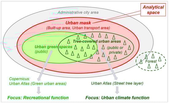
Figure 1.
Components of urban green infrastructure (own graphic).
The land use dataset of the first edition of the Urban Atlas 2006 was discussed in [22] when estimating spatial metrics to analyse the form of urban areas. For this purpose, the individual classes such as “Green urban areas” and “Sports and leisure facilities” were combined together into groups. The resulting analysis of nine Greek cities demonstrated the feasibility of applying such metrics to quantify the spatial structure and composition of land uses and thus provide insight into the underlying morphological characteristics of any city.
An international multi-city study by Ortí et al. (2022) offered a description of the taxonomic and structural diversity of woody vegetation in selected UGSs distributed across seven European cities from the northeast to the southwest [23]. The selection of UGSs was based on areas classified as “Green urban areas” in the second edition of the Urban Atlas 2012. With the help of additional data, over 400 woody species were identified in these areas. Their study provides information on the plant diversity and composition of woody vegetation in UGSs of different sizes, climates and urban planning history.
Exploring the nexus between urban dynamics, land use change and ecosystem services, Haase et al. (2018) investigated the topic of UGS development in European cities [24]. While many cities (mostly in Eastern Europe) are still shrinking today, others are now experiencing new growth. Both trends (shrinkage and growth) offer potential as well as risks for the sustainable use of urban land, including the provision of adequate green spaces. In their analysis of urban ecosystem services, Grunewald et al. (2019) investigated the provision and accessibility of UGSs in German cities using a multi-indicator approach [25].
Against the backdrop of green city concepts and with the aim of identifying and comparing green spaces in European cities, an indicator set was created by Engelhardt (2022). A corresponding dashboard was developed to analyse and visualise the spatial values—both for individual cities and in a comparison of European cities. The indicators for the quantity of green spaces were based on land use data from the Urban Atlas 2018, including both artificial spaces (especially green urban areas) and natural and semi-natural spaces (especially herbaceous vegetation and forests) [26]. This means that green spaces are included in the system both inside and outside the urban mask. Furthermore, there is a reference to green spaces for the population.
In the present study, the topic of urban greening and urban climate are addressed primarily with spatial reference to urban core areas as indicated by the unified urban masks described above. The author believes that this approach has largely been ignored in previous investigations, especially in study areas outside of Germany. Here, the calculation of city-wide UGS metrics is mainly based on European open geodata from the year 2018. The metrics include established indices from landscape ecology. By applying these to urban green structures, it is possible to uncover correlations between physiognomic features. European overview maps can provide information on whether and in which regions certain urban green structures dominate. While any general treatment of urban dynamics goes beyond the aim of this study, the structural analysis presented here offers a starting point for appropriate monitoring.
2. Materials and Methods
2.1. Study Area
A group of cities was selected from the member states of the European Environment Agency (EEA) to represent a wide geographical distribution or dispersity of urban structures throughout Europe. Base data were taken from the Copernicus Urban Atlas 2018 [27]. The study area consists of 30 cities within their administrative boundaries. A third of these are coastal cities, reflecting Europe’s distinctive and well-developed coastal areas. These sample cities were used in a previous study [8]; only the port city of Constanta on the Black Sea was replaced (due to inconsistencies in the 2018 Street Tree Layer data) with the Hanseatic city of Rostock on the Baltic Sea (providing an example city for additional comparison with two German geodatabases).
Care was taken to ensure that the administrative areas of the selected cities were spatially contiguous, i.e., without exclaves or islands (which were eliminated if necessary). Furthermore, the settlement site or urban mask of a city should be easily distinguishable from neighbouring municipalities. Therefore, megacities or large urban agglomerations of more than one million inhabitants were not included in the selection. A lower population boundary was set at 100,000 inhabitants, reflecting the usual definition of a large city. More than a quarter of the population of the EEA countries under consideration lives in cities of this size [28]. Together, these differently structured European cities constitute a sample set for the comparative analysis of UGSs. An overview of all selected cities is given in Table 1.

Table 1.
Overview of all selected cities in alphabetical order with population and area.
The spatial distribution of the case study cities in Europe can be seen in the overview maps of Section 3—where the results are presented (Figures 4, 9 and 13)—against the backdrop of biogeographical regions. The EEA has mapped 11 biogeographical regions of Europe at a scale of 1:1,000,000 and with a focus on biodiversity and sustainability [29]. In these overview maps, we can see eight of these regions: Alpine, Atlantic, Black Sea, Boreal, Continental, Mediterranean, Pannonian and Steppic. It is not always possible to unambiguously assign a city to a biogeographical region; there are often borderline cases or overlaps, such as in Bratislava (SK), Ljubljana (SI), Perugia (IT), Reims (FR) and Salzburg (AT). Therefore, the biogeographical regions are not used here for detailed analysis. Rather the map serves to locate the cities and provide a cartographic visualisation of the European context. Furthermore, the biogeographical regions play an important role in the validation of the European Copernicus data (level of reporting) [30].
2.2. Data Sources
All geodata used here are open geodata. This reflects the fundamental paradigm shift in recent years within society and public authorities as well as the economic and scientific sectors on the topic of data availability. Clearly, such discussions also apply to geodata [31].
As mentioned above, the main data source for this study is the Urban Atlas, which is part of the European Copernicus Land Monitoring Service. The Urban Atlas provides detailed vector data on land cover (LC) and land use (LU) for many of Europe’s urban regions. With a largely uniform nomenclature, these open data are available at a scale of 1:10,000 for the reference years 2006, 2012 and 2018. The latest 2018 edition provides high-resolution and inter-comparable geodata for 788 European city regions (“functional urban areas” or FUAs) [27]. These include all EU cities of more than 50,000 inhabitants along with their commuting zones. For the FUAs of the cities listed in Table 1, data from the 2018 edition of the Urban Atlas were used in this study (version v013; downloaded on 2 June 2022). A mapping guide contains the product description, mapping guidance and class description (28 classes) for the Urban Atlas [21]. Within the framework of the Copernicus Land Monitoring Service, the classification of the Urban Atlas is comparable to CORINE (Coordination of Information on the Environment) Land Cover.
From the 2012 edition onwards, the Urban Atlas has featured an additional layer for tree-covered areas over artificial surfaces. This so-called Street Tree Layer (STL) is a separate layer within artificial surfaces (level 1 urban mask) for each FUA. It details not only street trees but also contiguous rows or patches of trees covering 500 m² or more and with a minimum width of 10 m over this mask [21]. Various satellite images were interpreted to produce the 2018 edition of the STL (Pléiades, KOMPSAT, Planet, SPOT6, SuperView, etc.) [32]. With raster resolutions of 2 to 4 m, smoothing techniques were applied to these images to smooth the contours of the tree-covered areas and create the STL polygons. For the FUAs of the cities listed in Table 1, STL data from the 2018 edition of the Urban Atlas were used in this study (version v012; downloaded on 1 July 2022).
While the validation process of the Copernicus Urban Atlas 2018 edition (incl. STL) has not yet been completed, a validation report has already been issued [30]. One aspect of the validation process is to check whether these datasets comply with INSPIRE (Infrastructure for Spatial Information in the European Community) standards. The quality characteristics include completeness, logical consistency, positional accuracy, thematic accuracy, temporal quality and usability.
Within the framework of the European Urban Audit, annual population data are available for cities and so-called “greater cities”. To ensure temporal consistency with the Urban Atlas 2018 edition, corresponding values were selected from the Eurostat data table [28].
In addition, two German sources of open data were used for comparison, namely, the Urban Green Raster (UGR) Germany and tree data from a municipal tree register. The UGR is a land cover classification that addresses, in particular, the country’s areas of urban vegetation. The raster dataset has a spatial resolution of 10 m and is based on an automated classification of Sentinel-2 satellite data from the 2018 vegetation period [33]. The municipal tree register consists of point-based tree data from the Open Data Portal of the Hanseatic and University City of Rostock [34].
2.3. Spatial Analysis
Figure 2 gives an overview of this study’s methodology: from the input data to data preparation and analysis up to the presentation of the results. The urban mask derived from Copernicus data is central to the spatial or geometric relationships and the calculated city-wide UGS metrics (including correlation). The additional exemplary investigations using two German data sources are not shown in the figure.
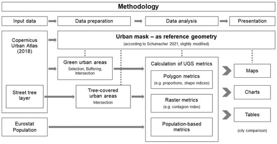
Figure 2.
Methodological overview of this study (own graphic).
As pointed out in the Introduction, certain core urban metrics on green infrastructure would be rendered more meaningful with spatial reference to an urban mask that reflects the German spatial element Ortslage rather than the administrative city area. As this spatial element is not considered outside of Germany, the author previously developed a GIS method to delineate such a layer at a medium scale using European Copernicus data [8]. To this end, the following land use classes were selected from the nomenclature of the Urban Atlas [21] as components for the urban mask:
- Continuous and discontinuous urban fabric (built-up area and associated land, predominantly residential structures) (classes 11100, 11210, 11220, 11230, 11240);
- Industrial, commercial, public, military, and private units (class 12100);
- Construction sites and land without current use (classes 13300, 13400);
- Green urban areas (public green areas for predominantly recreational use such as gardens, zoos, parks, castle parks and cemeteries) (class 14100);
- Sports and leisure facilities (class 14200).
Here, port areas were added to the list (class 12300). This extension appears necessary because port areas onshore include not only docking facilities but also associated industrial and commercial areas, which are not spatially separated in the database. In addition, dockyards are explicitly mapped as port areas.
In the Urban Atlas, road and rail transport is not differentiated according to whether the corresponding geo-objects are located within or outside the settlement area. Therefore, areas of inner-city transport can only be implicitly incorporated in the GIS algorithm for delineating the urban mask.
In this study’s workflow, the first step of data preparation is to select the category “Green urban areas” (class 14100) from the Urban Atlas data, which represents the publicly accessible UGS of a city. The category “Sports and leisure facilities” (class 14200) is not considered here because the related areas are usually significantly built-up/impervious and often inaccessible to the public. The map in Figure 3 shows the location of the public UGSs inside the urban mask as well as the forests in the open space in the city of Rostock, Germany. The determining factor in assigning an area to green urban areas is its public accessibility and close functional relationship to the built-up settlement areas according to the nomenclature of the Urban Atlas as mentioned above [21]. In the example of Rostock, a spatial concentration of green urban areas can be seen in the southwest of the city’s urban mask. The large forested area in the northeast of the administrative area (Rostocker Heide) is relatively far from the core settlement area of the city and thus not included in the urban mask.
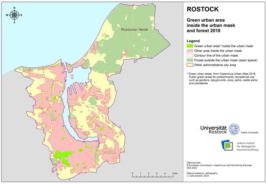
Figure 3.
City map of green urban areas inside the urban mask and forest in the open space of Rostock, Germany, 2018 (own processing).
As well as offering recreational services, the selected green urban areas have a beneficial microclimatic impact that generally radiates into adjacent structures. Therefore, these areas are externally buffered to a reasonable distance of 75 m (following a study on heat island and oasis effects of vegetative canopies [35]). This buffer distance, which is used by default, enables the mapping of the potential microclimatic effect of green urban areas, whereby constructional barriers are ignored [10]. Finally, the green urban areas including buffer zones intersect with the urban mask because all metrics considered here refer to this spatial unit.
An intersection with this reference geometry is also necessary for the data processing of the tree-covered open areas (Street Tree Layer). While the STL is clipped with an internal urban mask during its production, this is not published as open data within the framework of the Copernicus Land Monitoring Service and differs in detail from the urban mask used here [8,21].
The data analysis includes the calculation of selected metrics of UGSs (green urban areas or tree-covered urban areas) related to the urban mask for each city. In addition, all pairwise correlation coefficients between the selected variables are calculated. The metrics presented here are to be understood as examples. They were selected from the large number of available indices developed as part of the quantitative landscape analysis [36,37,38,39] as well as mathematical methods for urban ecology [40]. In the last-mentioned thesis by Thinh, green spaces within the settlement area (corresponding to an urban mask) are differentiated according to urban structure types and evaluated with suitable measurement variables.
This study focuses on the comparative application and analysis of metrics in the green–urban spatial context rather than developing a closed indicator system. Therefore, these metrics can be used here in their original units of measure. An extreme value normalisation such as in [10] is not carried out. Predominantly polygon-based metrics are calculated because the Copernicus input data are vector data. In the case of a raster-defined index, a vector–raster transformation is performed.
Table 2 gives an overview of all GIS-calculated variables or metrics with a general reference to the urban mask for the 30 European case study cities based on the Copernicus Urban Atlas data 2018. These city-wide characteristics can be divided into four groups: (I)—basic, (II)—public urban green, (III)—tree-covered urban green and (IV)—population-based. The variables in the last group also make use of population data from Eurostat [29]. The city-wide characteristics initially included simple variables such as absolute areas and area shares with reference to the urban mask. A vector-based and a raster-based index a selected from the extensive FRAGSTATS pool [36], respectively, and the Patch Analyst [37] as typical complex metrics:
Table 2.
City-wide characteristics with general reference to the urban mask.
- Area-weighted mean shape index (AWMSI) (No. 10);
- Contagion index (CI) (No. 11 and 14).
Both indices play an important role within the framework of the already-mentioned concept of urban metrics, where six main components are distinguished for the physiognomic analysis of urban structures: diversity, form complexity, heterogeneity, core area, neighbourhood and fragmentation [10]. The AWMSI is assigned to form complexity and the CI to form heterogeneity. Here, the indices are applied in a modified way, i.e., for the quantitative analysis of green structures within the urban mask. Both the shape complexity and the heterogeneity represent relevant physiognomic properties of urban green structures in the sense of urban morphology.
2.3.1. Area-Weighted Mean Shape Index (AWMSI)
The numerous metrics to describe the shape of polygons always consider the relation of edge lengths and areas. The area-weighted mean shape index is applied in this study as a measure of the shape complexity of landscape or settlement structures. Applied to urban metrics, this dimensionless index is calculated as follows [10]:
n = number of polygons;
i = index of polygons running from 1 to n;
Ei = perimeter length of polygon with index i;
Ai = area polygon with index i;
A = total area of polygons;
Range of values: [1; ∞].
A modified edge length–area ratio is considered, with larger areas carrying more weight than smaller ones in the calculation (increasing index values with the growing complexity of the structure). For the ideal shape of one single circular polygon, the measured value is one. A favourable property of the AWMSI is its low correlation to the size of the reference unit. This metric is applied here to characterise the form complexity of green urban areas within the urban mask of a city. If there are large public green spaces with jagged edges to the other (mostly built-up) areas within the urban mask, this is reflected in a high form complexity and a corresponding AWMSI index value. In order to preserve the shape of the original polygon boundaries and their fissuring, the buffer zones mentioned above are ignored here.
2.3.2. Contagion Index (CI)
The contagion index (degree of clumping) occupies a special position within heterogeneity metrics. This index describes the extent to which patches (e.g., green urban areas) are spatially aggregated or dispersed. It is therefore a raster-based index, where the respective grid cells are evaluated together with their neighbouring cells. For a given number of classes, the configuration of the grid cells is set in relation to their maximum possible spatial aggregation. The original formula was devised by O’Neill et al. [41]; the modified formula according to Li and Reynolds is used here [42]. The modified contagion index CI* as applied to urban metrics is calculated as follows [10]:
m = number of classes;
i, k = index of classes running from 1 to m;
Pi = proportion of spatial units occupied by an object of class i;
gik = number of pixel contacts of classes i and k;
Unit: %;
Range of values: (0; 100].
The formula can also be understood as a combination of two probabilities: the first corresponds to the probability that a randomly chosen pixel belongs to class i, derived from the proportional presence of this class in the calculated section; the second probability relates to the meeting of pixels of classes i and k. The combination corresponds to the probability that two randomly chosen neighbouring pixels belong to classes i and k [39]. The contagion index is 100% when all objects or pixels show their maximum spatial aggregation by class in the study area. In the case of maximum scattering (chessboard pattern, when each neighbouring cell has a different class), this index value tends to zero.
In the present application, the study area corresponds to the urban mask of a city. The Urban Atlas land use data are processed in such a way that only two spatially complementary classes remain: green urban areas and other areas inside the urban mask. Areas outside the urban mask are not considered. The contagion index of green urban areas inside the urban mask is calculated using the original data without any buffering. A high contagion index represents a strong spatial clumping or aggregation of green urban areas, and a low index represents their dispersed spatial distribution. Before the index can be calculated, these vector data must be transformed into raster data. The parameters for generating the raster dataset are oriented on the Urban Green Raster Germany (spatial resolution of 10 m) [33]. Both orthogonal and diagonal adjacent cells are regarded as connected cells (8-cell adjacency, chessboard distance).
The contagion index is also calculated for the tree-covered urban areas (STL) within the urban mask of a city. A high contagion index represents a strong spatial clumping or aggregation of tree-covered urban areas, while a low index represents their dispersed spatial distribution inside the urban mask.
2.3.3. Other Aspects
It makes little sense to calculate the AWMSI for the tree-covered urban areas as the STL often shows extremely complex and jagged shapes, which can change greatly with just slightly modified generalisation—with a relatively large influence on this index.
Of course, the spatial analyses must also incorporate a population reference. Therefore, city-wide population data from Eurostat are used here to calculate three metrics with a spatial reference to the urban mask (Table 2).
Finally, the results of the spatial analysis are presented in the form of maps, charts and tables. Cartographic visualisation at different scales and extents can greatly aid the recognition of spatial structures and planning conclusions. Here, we distinguish between European overview maps, city maps and detailed maps of city districts for specific purposes. The maps illustrate spatial characteristics of UGS in terms of their size, distribution and geometric structure in the urban core areas of European cities.
3. Results
All values calculated using the Copernicus data 2018 for the city-wide characteristics of the 30 selected European cities are compiled in the Supplementary Materials (Table S1). In addition, the pairwise correlation coefficients are included as a triangular matrix.
Here, we note considerable differences between the cities. In particular, the total population ranges between 119,000 in Cork, Ireland, and 965,000 in Marseille, France, while the administrative areas run from only 39.6 km² (also Cork) to 601.0 km² (also Marseille). However, the urban mask area is only moderately correlated with the administrative city area. Thus, the minimum and maximum values for the urban mask area are found in other cities: 30.5 km² in Burgos, Spain, and 255.6 km² in Toulouse, France. The number of separate urban mask polygons also varies greatly, namely, from only three in Cambridge, UK, to 427 in Angers, France. There is also a considerable disparity in the mean area of an urban mask polygon, with values ranging from 0.17 km² (Perugia, Italy) to 10.9 km² (Cambridge). The share of urban mask area to administrative city area ranges from 14.1% (Perugia) to 88.7% (Cork). These large value ranges related to the urban mask confirm the suitability of the selection of European cities for analysis (although, it should be pointed out that this sample is not statistically representative of all relevant European cities).
3.1. Green Urban Areas
The share of green urban area (inside the urban mask) to urban mask area 2018 for the selected case study cities is shown in an overview map in the context of the biogeographical regions of Europe (Figure 4). The individual cities show a wide range of values in the share of public urban green spaces, although, at first glance, no clear large-scale relationships are apparent. The location of a city on the coast or inland does not seem to play a role. On the other hand, city-specific characteristics of urban structures obviously have a considerable impact.
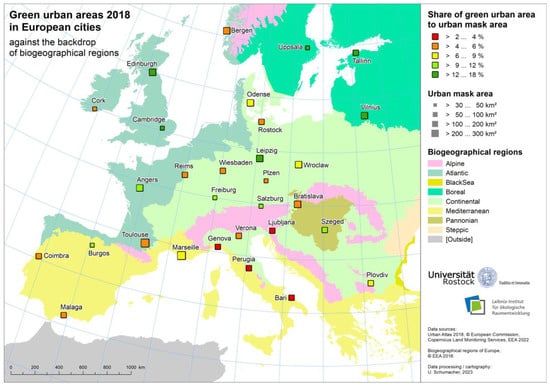
Figure 4.
Overview map of green urban areas 2018 in European cities against the backdrop of biogeographical regions (own processing).
The largest and smallest values of this city-wide measure already show regional trends: the share of green urban area to urban mask area varies greatly from 2.24% in Perugia (IT) to 17.95% in Vilnius (LT). All three case study cities in the Boreal biogeographical region—Vilnius (LT), Tallinn (EE) and Uppsala (SE)—have very high values. In contrast, three Italian cities from the Mediterranean region (Perugia, Genova, Bari) show very low values. With the inclusion of the 75 m buffer for the microclimatic impact zone, this share inside the urban mask increases substantially from 9.93% (Perugia) to 41.06% (Uppsala).
In Central Europe, the city of Leipzig, Germany, is characterised by a high number of large public urban green spaces (Figure 5). The share of green urban area within the urban mask is 14.96%. When including the potential microclimatic influence zones (+75 m buffer), this share more than doubles to 31.46%. Extensive parks, sports facilities and a zoological garden are located at the heart of a large alluvial forest, which stretches through the city from south to northwest. These green surfaces inside the urban mask run smoothly into the forest in the open space. Therefore, the delineation can vary depending on the geodata used, which has already been discussed for this case study in [8].
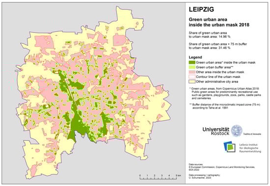
Figure 5.
City map of green urban area with buffer (potential microclimatic impact zone) inside the urban mask 2018 of Leipzig, Germany (own processing).
The chart in Figure 6 shows green urban areas and buffers of their potential microclimatic impact zones inside the urban mask of the case study cities 2018, arranged in ascending order according to the areal share of both green categories inside the urban mask. As absolute values are given, the chart reflects the different sizes of the case study cities (measured with their urban mask). As can be seen, the share of public urban green space (with or without a buffer zone) does not depend on the size of the city.
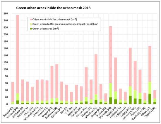
Figure 6.
Absolute values of green urban areas and buffers of their potential microclimatic impact zones inside the urban mask 2018 of the case study cities, arranged in ascending order according to the areal share of both green categories inside the urban mask (own processing).
As previously mentioned, the area-weighted mean shape index (AWMSI) of green urban area inside the urban mask is taken as a measure of the complexity of public urban green structures. The range of the index values is relatively small for the case study cities, lying between 1.539 for Verona, Italy, and 2.375 for Vilnius, Lithuania. Figure 7 shows two maps (at identical scale) of both cities with their green urban areas. The small range of AWMSI values means that the typical shape of the polygons of urban green structures deviates only slightly to moderately from a compact circular shape in all the cities examined. Those cities with a higher share of green urban areas inside the urban mask have larger and thus potentially more jagged and complex green spaces.
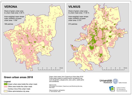
Figure 7.
City map of green urban area inside the urban mask 2018 of Verona, Italy, and Vilnius, Lithuania (own processing).
The correlation of the AWMSI to the other calculated variables is generally low, indicating its independent significance in this framework. The relationship between the AWMSI of green urban areas and the share of green urban areas to urban mask areas is presented in Figure 8a. The diagram shows a wide spread of cities in all directions and a low correlation between the two variables. The chart area is divided into four quadrants, with the division of abscissa and ordinate based on the mean values of the respective variables.
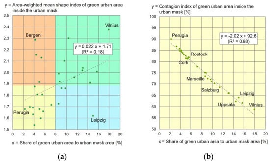
Figure 8.
Relationship between selected variables 2018 (own processing): (a) between the AWMSI of green urban area inside the urban mask and the share of green urban area to urban mask area and (b) between the contagion index of green urban area inside the urban mask and the share of green urban area to urban mask area.
In Figure 8a, a case study city is labelled towards the outer corner of each quadrant:
- Perugia, Italy: low share of green urban area to urban mask area and low AWMSI value of green urban area inside the urban mask;
- Bergen, Norway: low share of green urban area to urban mask area and high AWMSI value of green urban area inside the urban mask;
- Leipzig, Germany: high share of green urban area to urban mask area and low AWMSI value of green urban area inside the urban mask;
- Vilnius, Lithuania: high share of green urban area to urban mask area and high AWMSI value of green urban area inside the urban mask.
This provides a spectrum of public urban green structures in European cities specified over two dimensions, i.e., their areal proportion and the form complexity of their patches.
The contagion index (CI*) describes the degree of clumping, namely, the extent to which patches of green urban area occur spatially aggregated inside the urban mask of a city. The range of the index values for the case study cities lies between 59.14% (Vilnius, Lithuania) and 90.12% (Perugia, Italy). The strongest correlation of all city-wide characteristics from the triangular matrix (Supplementary Materials, Table S1) is found between the contagion index of green urban area inside the urban mask and the share of green urban area to urban mask area. The diagram in Figure 8b shows this very pronounced correlation (coefficient of determination R² = 0.98) with a negative linear regression coefficient, i.e., a continuously falling line. If the proportion of green urban areas is high (as in Vilnius), their spatial clumping is low and, consequently, the contagion index is relatively low because many large green patches are distributed within the urban mask of the city. In contrast, when the proportion of green urban areas is low (as in Perugia), their spatial clumping is high and, consequently, the contagion index is high because only a few small green patches are found within the urban mask of the city. The strength of this correlation seems surprising, especially since the calculation of the area share is based on vector data, while the calculation of the contagion index is performed after a raster transformation. Thus, if the share of green urban area within the urban mask is known, this already gives an indication of its spatial aggregation.
3.2. Tree-Covered Urban Areas
The share of tree-covered urban areas (inside the urban mask) to urban mask areas in 2018 for the selected case study cities is shown in an overview map in the context of the biogeographical regions of Europe (Figure 9). This share of tree cover (STL) varies greatly between the individual cities, whereby, at first glance, no clear large-scale relationships are apparent. The location of a city on the coast or inland does not seem to play any role. On the other hand, city-specific characteristics of urban structures obviously have a considerable impact. In Central Europe (mainly, the Continental biogeographical region), the selected cities consistently achieve high values for tree cover. In the Boreal biogeographical region, on the other hand, the two cities of Vilnius, Lithuania, and Uppsala, Sweden, record only average values. The cities in the Mediterranean region mostly show lower to average proportions of tree-covered areas inside the urban mask. The share of tree-covered urban areas varies widely from 3.27% in Verona, Italy, to 24.93% in Plzen, Czech Republic.

Figure 9.
Overview map of tree-covered urban areas 2018 in selected European cities against the backdrop of biogeographical regions (own processing).
Figure 10 shows maps of both cities (to the same scale) with their tree-covered areas indicated within the urban mask. The extensive tree population in Plzen is mainly located in the peripheral residential areas (private residential gardens and allotments). In contrast, there are very few tree-covered areas in the settlement areas of Verona due to the densely built-up medieval core and extensive industrial and commercial areas on the periphery, which are entirely without trees.
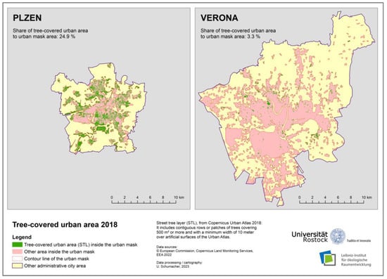
Figure 10.
City map of tree-covered urban area inside the urban mask 2018 of Plzen, Czech Republic, and Verona, Italy (own processing).
The chart in Figure 11 shows selected relative measures with reference to the urban mask. The case study cities are arranged in descending order according to the share of tree-covered urban areas to urban mask areas (from Plzen to Verona). We can see that the share of (public) green urban areas is only weakly correlated with the (public and private) share of tree-covered urban areas to urban mask areas (correlation coefficient r = 0.33). The two cities just mentioned differ only marginally in terms of their proportion of public green spaces. The very different share of the urban mask area to the administrative city area once again underlines the importance of the urban mask as a reference when calculating urban metrics for city-to-city comparison.
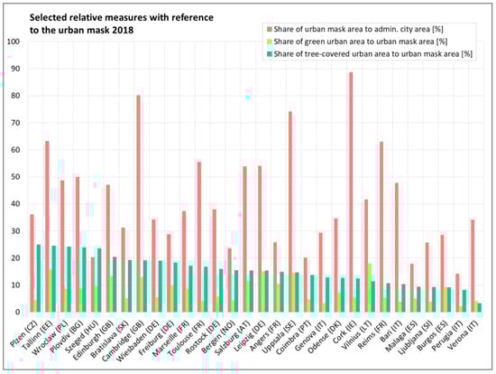
Figure 11.
Selected relative measures of the case study cities with reference to their urban mask 2018, arranged in descending order to the share of tree-covered urban area to urban mask area (own processing).
The share of tree-covered urban areas to urban mask areas shows only a weak to moderate correlation with other variables (Supplementary Materials, Table S1). Here, one should note the negative correlation to the number of separate polygons of the urban mask (correlation coefficient r = −0.42). Thus, a city with many, mostly smaller separate parts tends to have fewer tree-covered areas overall.
Figure 12 shows the relationship between the contagion index of tree-covered urban areas and the share of tree-covered urban areas to urban mask areas. As already mentioned, the contagion index indicates the degree of clumping, i.e., the extent to which patches of tree-covered urban areas occur spatially aggregated inside the urban mask of a city. The range of index values for the case study cities lies between 31.27% (Plzen, Czech Republic) and 84.02% (Verona, Italy). In Figure 12 we can see a very pronounced correlation (coefficient of determination R² = 0.97) with a negative sign for the linear regression coefficient, producing a continuously falling line. If the proportion of tree-covered urban areas is high (as in Plzen), their spatial clumping is low and, consequently, the contagion index is relatively low, reflecting the many large tree-covered patches distributed within the urban mask of the city. In contrast, when the proportion of tree-covered urban areas is low (as in Verona), their spatial clumping is high and, consequently, the contagion index is high, reflecting the few small tree-covered patches found within the urban mask of the city. Thus, if the proportion of tree-covered urban areas (similar to green urban areas) within the urban mask is known, this already gives an indication of its spatial aggregation in a city.
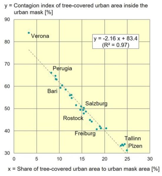
Figure 12.
Relationship between the contagion index of tree-covered urban areas inside the urban mask and the share of tree-covered urban areas to urban mask area 2018 (own processing).
3.3. Population-Based Metrics
Here, we examine the following population-based metrics with spatial reference to the urban mask to enable a city-to-city comparison: settlement density, green urban area per capita and tree-covered urban area per capita (results in the Supplementary Materials, Table S1).
Figure 13 gives an overview map of tree-covered urban areas (inside the urban mask) per capita for the case study cities against the backdrop of European biogeographical regions. There is a large variation in this population-based metric between the individual cities, whereby spatial relationships are only partially recognisable. The location of a city on the coast or inland does not seem to play a role here. On the other hand, city-specific characteristics of urban structures obviously have a considerable impact. The tree-covered urban area per capita varies widely between 0.86 ha/1000 inh. (Verona, Italy) and 9.66 ha/1000 inh. (Angers, France). In Central Europe (predominantly continental biogeographical region), the selected cities consistently achieve medium to high per capita values, whereas, in the Mediterranean region, they mostly show lower per capita values of tree-covered urban areas inside the respective urban mask.
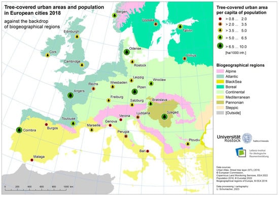
Figure 13.
Overview map of tree-covered urban areas per capita 2018 in selected European cities against the backdrop of biogeographical regions (own processing).
The highest positive correlation between the tree-covered urban area per capita and another metric is found with the green urban area per capita, although the correlation is fairly moderate (correlation coefficient r = 0.58). This underscores the interrelation and also the difference between public and private urban tree stocks, on the one hand, and public green urban areas, on the other. The highest negative correlation between the tree population per capita and the settlement density is only slightly higher (correlation coefficient = −0.69). Logically, larger tree-covered areas inside the urban mask are associated with lower settlement density. Otherwise, the correlations between the settlement density and other variables remain low to very low overall; the correlation coefficient for the share of the urban mask in the administrative city area even approaches zero, as the absolute minimum of the triangular matrix.
3.4. Significance of Correlation Values
All pairwise correlation coefficients between the calculated 17 city-wide characteristics with general reference to their urban masks are given in a triangular matrix (Supplementary Materials, Table S1). The absolute values of the linear correlation coefficients are between close to zero and close to one. The random maximum value of the correlation coefficient is r* = 0.36 (at 5% error probability for 30 case study cities, i.e., 28 degrees of freedom), tabulated in [43]. If the absolute value of the calculated coefficient r is smaller than the value r*, the null hypothesis can be assumed, namely, that there is no statistically reliable correlation between the spatial variables in question. This would have to be checked individually for all pairs of variables.
One surprising and non-trivial result is the strength of the inverse correlation between the “share of green urban area to urban mask area” and the “contagion index of green urban area inside the urban mask” (correlation coefficient r = −0.99). This also applies to the correlation between the “share of tree-covered urban area to urban mask area” and the “contagion index of tree-covered urban area inside the urban mask” (correlation coefficient r = −0.98). Thus, if the proportion of green urban areas or tree-covered urban areas within the urban mask is known, this already gives some indication of its spatial aggregation in a city. In this case, further empirical and theoretical investigations are indicated.
3.5. Additional Investigations
3.5.1. Exemplary Comparison with an Urban Green Raster
In addition to the European STL 2018, the Urban Green Raster (UGR) Germany (Stadtgrünraster Deutschland) can be used to spatially analyse tree-covered urban areas in Germany for the same reference year. The UGR data from the Leibniz Institute of Ecological Urban and Regional Development (IOER) is freely available at zenodo.org (publication date: 12 January 2022) and was downloaded for this study on 29 September 2022 [33]. As already mentioned in Section 2.2, the land use classification focuses on vegetation areas over the whole territory of Germany at a spatial resolution of 10 m. The dataset is based on an automated classification of Sentinel-2 satellite data from the vegetation period of 2018 using reference data from the European LUCAS (Land Use and Coverage Area frame Survey) point dataset. The UGR identifies eight land cover classes: built-up, built-up with significant green share, coniferous wood, deciduous wood, herbaceous vegetation (low perennial vegetation), water, open soil and arable land (low seasonal vegetation). A more detailed description of the UGR for indicator-based surveying of urban green space can be found in Eichler et al. (2020) [44].
After extracting the two tree-covered classes (coniferous and deciduous woods) from the UGR Germany and clipping them with the urban mask, a spatial comparison with the European STL data is useful. Figure 14 shows the overlay of the two geo-datasets in a map section with a spatial concentration of urban tree cover in the southwest of the city of Rostock.
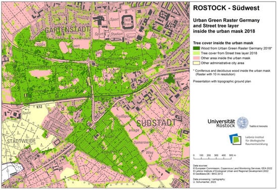
Figure 14.
Detailed map comparing tree cover derived from the Urban Green Raster Germany and from the European Street Tree Layer inside the urban mask 2018 of Rostock—Südwest (own processing).
While the area of tree cover within the urban mask of the whole city is found to be 5.28 km², as determined by the UGR, the area derived from the STL is almost twice as large at 10.23 km² (rasterised). The STL is clearly more finely structured than the UGR and contains numerous smaller tree-covered areas, but conversely, also contains more tree-free gaps. Here, the sensor type in the remote-sensing system used to gather the geodata certainly plays a significant role (STL with higher resolution than UGR, see Section 2.2). In addition, smaller tree-covered areas fall in the class “built-up with significant green share” in the UGR data. Further disparities result from the different pre-processing of the two databases. It should be noted that both these geo-datasets are used to generate the indicator “climate regulation in cities” as an ecosystem service in urban areas [45].
3.5.2. Exemplary Comparison with a Municipal Tree Register
In the online open data portal of the Hanseatic and University City of Rostock (OpenData.HRO), the tree register (Baumkataster) of the Office for Urban Greenery, Nature Conservation and Cemeteries (Amt für Stadtgrün, Naturschutz und Friedhofswesen) can be found under the German keyword “Bäume”. The municipal dataset was downloaded for this study on 6 January 2023 [34]. It will be used here as an example for comparison with European geodata on the urban tree population. In the textbook Grundlagen der Geo-Informationssysteme, a tree or green space register is characterised as documenting the tree, green and park space inventory of a municipality, thereby contributing to the preservation of the natural function of the green spaces and serving as a planning instrument for land maintenance measures [46] (pp. 743–744).
The Rostock dataset contains the point-located trees of the register along with information on the genus, species, status as a street tree, height, trunk diameter, trunk circumference and crown diameter. The data used here (WFS, processing status 6 January 2023) correspond approximately to the status at the end of the year 2022. Compared with European Copernicus data 2018, this gives a temporal disparity of approximately four years.
A total of 71,070 trees are geocoded as points in the register, of which 69,137 trees are located in the administrative city area. After the GIS intersection of this point layer with the urban mask of Rostock based on the Copernicus Urban Atlas 2018 (modified urban mask, see Section 2.3), 56,311 trees remain for further analysis. There are also missing points in the recorded tree attributes, such as the crown diameter in approx. 3% of all cases in the city area. However, this attribute is required to create a tree cover area layer by buffering the point data. For this reason, the average crown diameter of all other trees (6.3 m) was assumed when values were missing. The unified polygon layer of all tree crowns (tree cover) is cartographically shown in combination with the Copernicus Street Tree Layer (STL) 2018 for a section in the southwest of the Rostock city area (Figure 15).
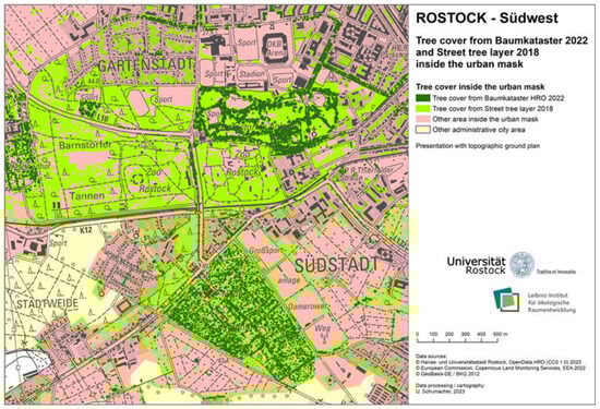
Figure 15.
Detailed map of the tree cover from the Baumkataster Rostock 2022 and the European Street Tree Layer (STL) inside the urban mask 2018 in Rostock—Südwest (own processing).
Significant differences between the two geodatabases are clearly visible. The European STL (parameters see Section 2.2) is much more generously delineated or more generalised than the tree cover (based on terrestrial individual tree recording) from the municipal tree register. While the STL maps the tree population across the entire urban mask (public and private areas), the tree register has gaps (e.g., in Rostock Zoo, in other sports and leisure facilities, residential areas, industrial and commercial areas, port facilities, allotment garden sectors and military facilities). Using the satellite data, it is likely to be more difficult to distinguish between trees and shrubs, resulting in a coarser demarcation of tree groups in the STL. Spatially separate individual trees, which are generally recorded in the register, sometimes fall below the detection limit for the STL (min. of 500 m² of contiguous tree cover), although these have only a minor influence on the total area of the cover. Street trees are included in the municipal register independently of the urban mask, whereby the trees in open spaces (e.g., street trees on connecting roads between separate parts of the urban mask) are not considered in the present comparison.
Further information on the tree register from the tree inspector of the Office for Urban Greenery, Nature Conservation and Cemeteries of Rostock can aid in the interpretation of the results [47]:
- Tree crown diameter: estimation with visual inspection or determined by the number of steps taken by a surveyor stepping from the trunk to the perimeter of the crown (averaging with asymmetrical crown shape);
- Full update: approx. every five years (new data introduced approx. every three days);
- Area coverage: trees managed by the municipal real estate office (no private areas such as Rostock Zoo).
A detailed investigation in a test area was undertaken to provide more information on canopy delineation in comparison. The Neuer Friedhof, a cemetery located in the southwest of Rostock, was selected for this purpose: this site is within the urban mask and has its tree population that is fully recorded in both databases. The cemetery can be clearly extracted as an intersection polygon from the Urban Atlas (scale 1:10,000). This classified green urban area is found to contain a total of 3291 trees of 87 different species from the tree register. Such a high spatial density of vegetation is typical for a Central European cemetery. Figure 16 shows a map of the unified polygon layer of all tree crowns in the test area drawn from the register (tree cover), overlaid with tree cover taken from the European STL.
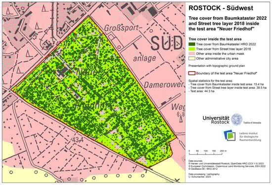
Figure 16.
Detailed map of the tree cover from the Baumkataster Rostock 2022 and the European Street Tree Layer (STL) 2018 inside the test area “Neuer Friedhof” (own processing).
The proportion of tree cover in the cemetery determined from the Street Tree Layer (89.2%) is more than 2.5 times higher than in the figure derived from the tree register (34.8%). Due to the more generalised nature of the STL—as explained above—the real tree cover is probably overestimated. Conversely, only 3.6% of the tree points from the register lie outside the STL polygon in the test area. The difference in the time reference between the two databases does not provide a plausible explanation for the considerable difference in area (crown growth versus tree maintenance or dieback in four years). No open data are yet available from the tree register at several fixed points in time, which would be a precondition for monitoring.
4. Discussion
A comprehensive bibliometric analysis of UGS research over the last three decades by Farkas et al. (2023) found that scientific studies have increasingly focused on inner-city areas. The worldwide densification of urban areas, also in industrialised countries, is often accompanied by the disappearance of existing green spaces. At the same time, research has highlighted the benefits and positive impacts of UGSs on urban residents [48]. These trends support the approach of studies that make spatial reference to urban masks in the sense discussed here.
The aggregation and delineation of contiguous built-up areas along with other areas closely related both functionally and spatially to settlements, as realised by an urban mask (according to the Ortslage feature class of the German authoritative topographic base datasets), may be useful for various analyses and planning tasks that focus on urban core spaces (see the Introduction). In such cases, the urban mask area seems more suitable as a reference unit for the city as a whole than its administrative area. Here, any decision on the relevant reference unit should always be made to reflect the focus of interest. This also concerns the application of urban metrics in the context of UGS—for example, when analysing urban heat islands.
In any study on this topic, the UGS must be clearly defined in terms of content and space from the outset, especially since this term can have different meanings in the literature [20]. In the present study, we are considering green spaces in urban core areas of European cities. As described in the Introduction, a distinction is made between (public) green urban areas and (public and private) tree-covered urban areas within the urban mask—with both categories from European Copernicus data overlapping spatially.
The analysis of UGSs presented here based on open geodata for selected cities with a general reference to unified urban masks does not represent a self-contained system but rather an open approach. This means that the characteristics, variables or metrics used for the quantitative description of green spaces within the urban mask of a city are exemplary and chosen with regard to essential city-wide statements. In particular, they can be complemented by further aspects and be introduced into a multi-criteria assessment system, as shown by a previous complex study that made use of topographic geodata to examine German cities [10].
In the current study, a single category of the Copernicus Urban Atlas, namely, public urban green spaces (green urban areas), was specifically selected because only these areas are publicly accessible, minimally sealed and located inside the urban mask. However, there exist uncertainties in the delineation of the urban mask to open space (especially to the forest, without a clear definition), which is noted in the validation report [30]. This affects the UGS-related metrics and must be taken into account when interpreting the values for the 2018 edition. Here, improvements can be expected for future editions of the Urban Atlas.
In the context of urban climate functions, geo-information on the tree population is required, primarily within urban core areas, and mapped by the urban mask of a city. Here, the properties (plots of land) concerned, their owners and accessibility do not play a role. In principle, the Street Tree Layer (STL) of the Copernicus Urban Atlas is suitable for this purpose, as it contains not only the tree-covered area inside the street space but all trees within artificial surfaces. These vector data are also available for almost 800 European city regions (FUA) as open data, enabling the medium-scale comparative spatial analyses of urban tree cover in European cities. For the reference year 2018, such partially validated data are based on satellite images at higher resolution (2 to 4 m). In visual comparison, the new STL polygons appear more finely structured than the STL polygons of the first edition from 2012, which is likely to be problematic in terms of monitoring.
The comparison of different geo-datasets on UGSs could provide helpful insights into their characteristics, such as are rendered visible when two urban tree-cover datasets are overlaid. The statistical, spatial–structural and visual comparison of a German dataset (UGR) with the European dataset (STL) already shows clear differences for one example city in the same reference year and also suggests ways of improving both datasets—for example, using data fusion.
When comparing the European STL data with the derived tree canopy cover from a municipal tree register, large quantitative differences become apparent even in a suitable test area. This is due to the very different purposes of both geo-datasets and the resulting acquisition methods (remote sensing versus field acquisition) as well as data structures (polygons versus points). In addition, the focus of the tree register is on identifying individual trees, classified by species and other attributes. It can be assumed that the local authorities of European cities use very different approaches when setting up their tree registers. Therefore, the European STL could at best be used as an auxiliary source of spatial information to help validate a tree register.
5. Conclusions
The results of this study are city-wide values for the characterisation of public urban green spaces as well as tree-covered urban green spaces (public or private) with general reference to unified urban masks of 30 selected European cities displaying a wide range of urban structures (Supplementary Materials, Table S1). In addition to simple shared values, two established complex indices were calculated as examples—shape complexity (vector-based) and heterogeneity (raster-based). Furthermore, three population-based metrics were determined. In general, the values of the UGS metrics vary considerably between the individual cities with no clear large-scale relationships initially apparent. Obviously, city-specific factors will strongly influence the urban structures of historically developed cities in Europe. The spatial reference to unified urban masks places the analytical focus of city-wide metrics onto corresponding core areas. In general, no statistically significant correlations between the share of green urban areas (or the share of tree-covered urban areas) to the absolute urban mask area could be found. Of particular interest is the very high correlation between the share value and the contagion index (of both green urban areas and tree-covered urban areas): if this share within the urban mask is known, it already gives an indication of the spatial aggregation of UGS in a city.
The overview maps of European cities presented in this paper show biogeographical regions delineated by the EEA, which indicate a wide variety of habitat types and ecosystems mapped on a continental scale. With such maps, it is possible to reveal relationships between the biodiversity mapped in the region and the structure of UGSs in the cities. However, this would require more in-depth analyses for a larger number of cities that can be clearly assigned to a single biogeographical region. In this context, the European overview map of tree-covered urban area per capita (Figure 13) should be mentioned here: in the Mediterranean region, for example, values tend to be quite low, reflecting both the dense shaded built environment and the predominant tree species. From the city maps, further conclusions can be drawn for urban green planning in terms of spatial structure, distribution and connectivity of UGSs. The detailed maps of city districts, city maps and European overview maps can be integrated into an open dashboard system with corresponding diagrams and value tables [49]—following a proposal by Engelhardt (2022) [26]. Such a green city dashboard is intended to raise people’s awareness of the importance of public UGSs and trees in urban areas.
The use of uniformly produced and validated vector data from the Copernicus Land Monitoring Service according to INSPIRE standards potentially provides a solid basis for the comparative analysis of almost 800 European cities (each with more than 50,000 inhabitants), including their surrounding functional urban areas (FUAs). In addition, investigations of urban sub-areas (city districts, parcels of land according to the cadastre or areas delineated in terms of settlement structure) are possible and useful. The provision of open data is a prerequisite for transparent scientific research, planning processes and public information.
As emphasised by the author [8], a uniformly generated, comparable and openly available urban mask would be a great boon to cross-border studies—for example, in the context of the European Urban Audit. This novel spatial reference (reflecting the German Ortslage) can support UGS analyses in urban core areas of European cities based on comparable open datasets, as exemplified here. The regular updating of the Urban Atlas data every six years within the Copernicus Land Monitoring Service opens up the possibility of integrating such analyses into the European Spatial Observation. This monitoring would aid a structural enhancement in green spaces in urban core areas, which have an essential role to play in adapting to climatic changes, in particular, the heatwaves and extended periods of drought that undermine the health and well-being of urban residents.
To quantify the urban heat island effect, meteorological point data from georeferenced stations are needed covering long periods of time—in a study by Possega et al. (2022), for example, for 37 European cities over a period of 20 years were needed [50]. When selecting meteorological stations, it is necessary to choose urban and rural stations on a uniform geodatabase, which requires the definition of an urban mask. The temperature difference between city centres and the surrounding countryside, especially in the summer months and at night, is mainly due to the properties of urban surfaces. Here, information can be derived to assess the efficiency of UGSs in mitigating the impact of extreme heat events, underscoring the crucial role of tree cover in thermal comfort regulation. To support such investigations, the delineation of a unified urban mask could be a useful contribution.
For further studies, additional spatial variables (both natural and anthropogenic) should be included to better assess UGS development in individual cities and to be able to draw corresponding planning conclusions. When combining European UGS geodata with local geodata (for example, derived tree cover from an urban tree register), larger deviations are to be expected, which will accordingly affect a corresponding data fusion.
Furthermore, the Copernicus data portfolio has for several years provided some high-resolution layers (HRLs) for specific land cover and land use characteristics, namely: imperviousness, forest, grassland, water and wetness and small woody features. In the near future, these open and harmonised HRL geodata will be incorporated into a new category called “Vegetated Land Cover Characteristics (VLCC)” [51]. The urban mask model should also be considered in this context—within the green land monitoring of city regions in Europe.
Supplementary Materials
The following supporting information can be downloaded at: https://www.mdpi.com/article/10.3390/land13010027/s1, Table S1: Basic shape characteristics and population of selected European cities 2018 (incl. correlation matrix).
Funding
This research received no external funding.
Data Availability Statement
The data presented in this study are openly available in Copernicus Land Monitoring Services (CLMS): Urban Atlas 2018. Available online: https://land.copernicus.eu/local/urban-atlas/urban-atlas-2018 (accessed on 2 June 2022); Copernicus Land Monitoring Services (CLMS): Street Tree Layer 2018. Available online: https://land.copernicus.eu/local/urban-atlas/street-tree-layer-stl-2018 (accessed on 1 July 2022); European Environment Agency (EEA): Biogeographical regions in Europe. Available online: https://www.eea.europa.eu/data-and-maps/data/biogeographical-regions-europe-3 (accessed on 2 September 2022); Eurostat: Population on 1 January by age groups and sex—cities and greater cities. Available online: https://ec.europa.eu/eurostat/web/products-datasets/-/urb_cpop1 (accessed on 6 April 2023); Leibniz-Institut für ökologische Raumentwicklung (IÖR): Urban Green Raster Germany 2018. Zenodo, 2022. Available online: https://doi.org/10.26084/ioerfdz-r10-urbgrn2018 (accessed on 29 September 2022); Hanse-und Universitätsstadt Rostock: OpenData.HRO. Bäume des Baumkatasters Rostock. Available online: https://www.opendata-hro.de/dataset/baeume (accessed on 6 January 2023).
Acknowledgments
The author thanks Ralf Bill (Rostock), Nguyen X. Thinh (Dortmund), Tobias Krüger, Georg Schiller and Juliane Mathey (all Dresden) for their critical comments on the manuscript. Furthermore, the author would like to thank the reviewers for their constructive feedback. Thanks also go to Derek Henderson for the proofreading.
Conflicts of Interest
The author declares no conflict of interest.
Software Availability
ESRI ArcGIS Desktop 10.8.2 incl. Patch Analyst extension 5.2.0.16; Fragstats 4.2.1.603.
References
- United Nations (UN). Transforming Our World: The 2030 Agenda for Sustainable Development. 2015. Available online: https://sustainabledevelopment.un.org/content/documents/21252030%20Agenda%20for%20Sustainable%20Development%20web.pdf (accessed on 20 November 2023).
- European Environment Agency (EEA). Who Benefits from Nature in Cities? Social Inequalities in Access to Urban Green and Blue Spaces across Europe. 2022. Available online: https://www.eea.europa.eu/publications/who-benefits-from-nature-in (accessed on 20 November 2023).
- Ugolini, F.; Massetti, L.; Calaza-Martínez, P.; Cariñanos, P.; Dobbs, C.; Krajter Ostoić, S.; Marin, A.M.; Pearlmutter, P.; Saaroni, H.; Šaulienė, I.; et al. Effects of the COVID-19 pandemic on the use and perceptions of urban green space: An international exploratory study. Urban For. Urban Green. 2020, 56, 126888. [Google Scholar] [CrossRef] [PubMed]
- European Environment Agency (EEA). Urban Tree Cover in Europe. Dashboard (Tableau). 2021. Available online: https://www.eea.europa.eu/data-and-maps/dashboards/urban-tree-cover (accessed on 20 November 2023).
- Schwab, J.; Meier, R.; Mussetti, G.; Seneviratne, S.; Bürgi, C.; Davin, E.L. The role of urban trees in reducing land surface temperatures in European cities. Nat. Commun. 2021, 12, 6763. [Google Scholar] [CrossRef] [PubMed]
- Arbeitsgemeinschaft der Vermessungsverwaltungen der Länder der Bundesrepublik Deutschland (AdV). Dokumentation zur Modellierung der Geoinformationen des amtlichen Vermessungswesens (GeoInfoDok). ATKIS-Objektartenkatalog Basis-DLM. Version 7.1 rc.1. Germany. 2018. Available online: http://www.adv-online.de/icc/extdeu/nav/a63/binarywriterservlet?imgUid=9201016e-7efa-8461-e336-b6951fa2e0c9&uBasVariant=11111111-1111-1111-1111-111111111111 (accessed on 28 September 2022).
- Leibniz Institute of Ecological Urban and Regional Development (IOER). Monitor of Settlement and Open Space Development. Glossary. Dresden, Germany. 2023. Available online: https://www.ioer-monitor.de/en/methodology/glossary/u/urban-site (accessed on 20 November 2023).
- Schumacher, U. The Urban Mask Layer as Reference Geometry for Spatial Planning: Moving from German to European Geodata. KN J. Cartogr. Geogr. Inf. 2021, 71, 83–95. [Google Scholar] [CrossRef]
- Pourtaherian, P.; Jaeger, J.A.G. How effective are greenbelts at mitigating urban sprawl? A comparative study of 60 European cities. Landsc. Urban Plan. 2022, 227, 104532. [Google Scholar] [CrossRef]
- Deilmann, C.; Lehmann, I.; Schumacher, U.; Behnisch, M. Stadt im Spannungsfeld von Kompaktheit, Effizienz und Umweltqualität. Anwendungen urbaner Metrik; Springer: Berlin/Heidelberg, Germany, 2017; 231p. [Google Scholar] [CrossRef]
- Frick, A.; Wagner, K.; Kiefer, T.; Tervooren, S. Wo fehlt Grün?—Defizitanalyse von Grünvolumen in Städten. In Flächennutzungsmonitoring XII mit Beiträgen zum Monitoring von Ökosystemleistungen und SDGs; IÖR Schriften 78; Meinel, G., Schumacher, U., Behnisch, M., Krüger, T., Eds.; Rhombos: Berlin, Germany, 2020; pp. 223–238. [Google Scholar] [CrossRef]
- Bundesinstitut für Bau-, Stadt- und Raumforschung (BBSR). Wie grün sind deutsche Städte? BBSR-Online-Publikation, 03/2022. Available online: https://www.bbsr.bund.de/BBSR/DE/veroeffentlichungen/bbsr-online/2022/bbsr-online-03-2022.html (accessed on 20 November 2023).
- Institut für Landes- und Stadtentwicklungsforschung (ILS). Incora—Inwertsetzung von Copernicus-Daten für die Raumbeobachtung: Indikator “Vegetationsbedeckung innerhalb von Ortslagen”. Dortmund, Germany. 2022. Available online: https://incora-flaeche.de/indikatoren/veraenderung-stadtgruen (accessed on 20 November 2023).
- Fina, S.; Eichfuss, S.; Xu, S.; Riembauer, G.; Dosch, F. Das Dashboard incora-flaeche.de zum Vergleich von Flächennutzungs- und Landbedeckungsdaten. gis.Science 2023, 36, 28–38. Available online: https://gispoint.de/artikelarchiv/gis/2023/gisscience-ausgabe-12023/7674-das-dashboard-incora-flaechede-zum-vergleich-von-flaechennutzungs-und-landbedeckungsdaten.html (accessed on 20 November 2023).
- Colding, J.; Gren, A.; Barthel, S. The Incremental Demise of Urban Green Spaces. Land 2020, 9, 162. [Google Scholar] [CrossRef]
- Mathey, J.; Hennersdorf, J.; Lehmann, I.; Wende, W. Qualifying the urban structure type approach for urban green space analysis—A case study of Dresden, Germany. Ecol. Indic. 2021, 125, 107519. [Google Scholar] [CrossRef]
- Pezzagno, M.; Frigione, B.M.; Ferreira, C.S.S. Reading Urban Green Morphology to Enhance Urban Resilience: A Case Study of Six Southern European Cities. Sustainability 2021, 13, 9163. [Google Scholar] [CrossRef]
- Valente, D.; Marinelli, M.V.; Lovello, E.M.; Giannuzzi, C.G.; Petrosillo, I. Fostering the Resiliency of Urban Landscape through the Sustainable Spatial Planning of Green Spaces. Land 2022, 11, 367. [Google Scholar] [CrossRef]
- Wolff, M.; Haase, D.; Priess, J.; Hoffmann, T.L. The Role of Brownfields and Their Revitalisation for the Functional Connectivity of the Urban Tree System in a Regrowing City. Land 2023, 12, 333. [Google Scholar] [CrossRef]
- Taylor, L.; Hochuli, D. Defining greenspace: Multiple uses across multiple disciplines. Landsc. Urban Plan. 2017, 158, 25–38. [Google Scholar] [CrossRef]
- European Union (EU). Mapping Guide for a European Urban Atlas. V 6.2. 2020. Available online: https://land.copernicus.eu/user-corner/technical-library/urban_atlas_2012_2018_mapping_guide/view (accessed on 20 November 2023).
- Prastacos, P.; Lagarias, A.; Chrysoulakis, N. Using the Urban Atlas dataset for estimating spatial metrics. Methodology and application in urban areas of Greece. Cybergeo Eur. J. Geogr. 2017, 22, 815. [Google Scholar] [CrossRef]
- Ortí, M.A.; Casanelles-Abella, J.; Chiron, F.; Deguines, N.; Hallikma, T.; Jaksi, P.; Kwiatkowska, P.K.; Moretti, M.; Muyshondt, B.; Niinemets, Ü.; et al. Negative relationship between woody species density and size of urban green spaces in seven European cities. Urban For. Urban Green. 2022, 74, 127650. [Google Scholar] [CrossRef]
- Haase, A.; Wolff, M.; Rink, D. From Shrinkage to Regrowth: The Nexus Between Urban Dynamics, Land Use Change and Ecosystem Service Provision. In Urban Transformations; Future City; Kabisch, S., Koch, F., Gawel, E., Haase, A., Knapp, S., Krellenberg, K., Nivala, J., Zehnsdorf, A., Eds.; Springer: Cham, Germany, 2018; Volume 10. [Google Scholar] [CrossRef]
- Grunewald, K.; Richter, B.; Behnisch, M. Multi-Indicator Approach for Characterising Urban Green Space Provision at City and City-District Level in Germany. Int. J. Environ. Res. Public Health 2019, 16, 2300. [Google Scholar] [CrossRef] [PubMed]
- Engelhardt, L. Entwicklung und Konzeption eines Dashboards zur Präsentation eines Grünraum-Indikatorsystems für europäische Städte. gis.Science 2022, 35, 97–108. Available online: https://gispoint.de/artikelarchiv/gis/2022/gisscience-ausgabe-32022/7619-entwicklung-und-konzeption-eines-dashboards-zur-praesentation-eines-gruenraum-indikatorsystems-fuer-europaeische-staedte.html (accessed on 20 November 2023).
- Copernicus Land Monitoring Service (CLMS). Urban Atlas 2018. Available online: https://land.copernicus.eu/local/urban-atlas/urban-atlas-2018 (accessed on 2 September 2022).
- Eurostat. Population on 1 January by Age Groups and Sex—Cities and Greater Cities. Available online: https://ec.europa.eu/eurostat/web/products-datasets/-/urb_cpop1 (accessed on 6 April 2023).
- European Environment Agency (EEA). Biogeographical Regions in Europe. Available online: https://www.eea.europa.eu/data-and-maps/data/biogeographical-regions-europe-3 (accessed on 2 September 2022).
- Copernicus Land Monitoring Service (CLMS). Urban Atlas 2018 Validation Report. Issue 1.6. Available online: https://land.copernicus.eu/user-corner/technical-library/urban-atlas-2018-validation-report (accessed on 2 September 2022).
- Bill, R. Offene Geodaten—Ein Paradigmenwechsel. In GIS-Report 2018/2019; Harzer: Karlsruhe, Germany, 2018; pp. 9–15. Available online: https://www.opengeoedu.de/Content/Publikationen/GISReport2018.pdf (accessed on 20 November 2023).
- Copernicus Land Monitoring Service (CLMS). Street Tree Layer 2018. Available online: https://land.copernicus.eu/local/urban-atlas/street-tree-layer-stl-2018 (accessed on 2 September 2022).
- Krüger, T.; Eichler, L.; Meinel, G.; Tenikl, J.; Taubenböck, H.; Wurm, M. (IÖR) Urban Green Raster Germany 2018. Zenodo, 2022. Available online: https://doi.org/10.26084/ioerfdz-r10-urbgrn2018.
- Hanse- und Universitätsstadt Rostock (HRO). OpenData.HRO. Bäume des Baumkatasters. Rostock, Germany, 2023. Available online: https://www.opendata-hro.de/dataset/baeume (accessed on 6 January 2023).
- Taha, H.; Akbari, H.; Rosenfeld, A. Heat Island and Oasis Effects of Vegetative Canopies: Micro-Meteorological Field-Measurements. Theor. Appl. Climatol. 1991, 44, 123–138. [Google Scholar] [CrossRef]
- McGarigal, K.; Marks, B.J. FRAGSTATS: Spatial Pattern Analysis Program for Quantifying Landscape Structure; General technical report. PNW-GTR-351; U.S. Department of Agriculture, Forest Service, Pacific Northwest Research Station: Portland, OR, USA, 1995. [CrossRef]
- Rempel, R.S.; Kaukinen, D.; Carr, A.P. Patch Analyst and Patch Grid. Ontario Ministry of Natural Resources. Centre for Northern Forest Ecosystem Research, Thunder Bay, Ontario, Canada, 2012. Available online: https://patch-analyst.software.informer.com/download (accessed on 2 September 2022).
- Walz, U. Landschaftsstrukturmaße und Indikatorensysteme zur Erfassung und Bewertung des Landschaftswandels und seiner Umweltauswirkungen—Unter besonderer Berücksichtigung der biologischen Vielfalt; Habilitation; Universität Rostock: Rostock, Germany, 2013. [Google Scholar]
- Lang, S.; Blaschke, T. Landschaftsanalyse mit GIS; Ulmer: Stuttgart, Germany, 2007; 405p. [Google Scholar]
- Thinh, N.X. Entwicklung von Mathematisch-Geoinformatorischen Methoden und Modellen zur Analyse, Bewertung, Simulation und Entscheidungsunterstützung in Städtebau und Stadtökologie; Habilitation; Universität Rostock: Rostock, Germany, 2005. [Google Scholar]
- O’Neill, R.V.; Krummel, J.R.; Gardner, R.H.; Sugihara, G.; Jackson, B.; DeAngelis, D.L.; Milne, B.T.; Turner, M.G.; Zygmunt, B.; Christensen, S.W.; et al. Indices of landscape pattern. Landsc. Ecol. 1988, 1, 153–162. Available online: https://www.lapa.ufscar.br/geotecnologias-1/O%20NEILL%2088_indices_of_landscape_pattern.pdf (accessed on 20 November 2023). [CrossRef]
- Li, H.; Reynolds, J.F. A new contagion index to quantify spatial patterns of landscapes. Landsc. Ecol. 1993, 8, 155–162. Available online: https://andrewsforest.oregonstate.edu/sites/default/files/lter/pubs/pdf/pub1502.pdf (accessed on 20 November 2023). [CrossRef]
- Storm, R. Wahrscheinlichkeitsrechnung, Mathematische Statistik und Statistische Qualitätskontrolle; VEB Fachbuchverlag: Leipzig, Germany, 1974. [Google Scholar]
- Eichler, L.; Krüger, T.; Meinel, G.; Tenikl, J.; Wurm, M. Wie grün sind deutsche Städte? Indikatorgestützte fernerkundliche Erfassung des Stadtgrüns. AGIT—J. Für Angew. Geoinformatik 2020, 6, 306–315. [Google Scholar] [CrossRef]
- Meier, S.; Syrbe, R.U.; Moyzes, M.; Grunewald, K. Klimaregulation in Städten als Ökosystemleistung. Vorschlag eines nationalen Indikators zur Bewertung der Ökosystemleistung Klimaregulation in Städten. Naturschutz Landschaftsplanung 2022, 54, 20–29. [Google Scholar] [CrossRef]
- Bill, R. Grundlagen der Geo-Informationssysteme, 7th ed.; Wichmann/VDE: Berlin, Germany, 2023; 901p. [Google Scholar]
- Fietkau, C. (Amt für Stadtgrün, Naturschutz und Friedhofswesen, Hanse- und Universitätsstadt Rostock, Germany). Personal communication, 2023. [Google Scholar]
- Farkas, J.Z.; Hoyk, E.; Batista de Morais, M.; Csomos, G. A systematic review of urban green space research over the last 30 years: A bibliometric analysis. Heliyon 2023, 9, e13406. [Google Scholar] [CrossRef] [PubMed]
- ESRI. European Green Cites Dashboard, 2022. Available online: https://www.arcgis.com/apps/dashboards/56ff8bb398dd4e9291f461a2bae5d455 (accessed on 20 November 2023).
- Possega, M.; Aragão, L.; Ruggieri, P.; Santo, M.A.; Di Sabatino, S. Observational evidence of intensified nocturnal urban heat island during heatwaves in European cities. Environ. Res. Lett. 2022, 17, 124013. [Google Scholar] [CrossRef]
- Copernicus Land Monitoring Service (CLMS). OBSERVER: Vegetated Land Cover Characteristics (VLCC): A New Era of Land Monitoring (29/06/2023). Available online: https://www.copernicus.eu/en/news/news/observer-vegetated-land-cover-characteristics-vlcc-new-era-land-monitoring (accessed on 20 November 2023).
Disclaimer/Publisher’s Note: The statements, opinions and data contained in all publications are solely those of the individual author(s) and contributor(s) and not of MDPI and/or the editor(s). MDPI and/or the editor(s) disclaim responsibility for any injury to people or property resulting from any ideas, methods, instructions or products referred to in the content. |
© 2023 by the author. Licensee MDPI, Basel, Switzerland. This article is an open access article distributed under the terms and conditions of the Creative Commons Attribution (CC BY) license (https://creativecommons.org/licenses/by/4.0/).