Article

A Proposed Methodology for Determining the Economically Optimal Number of Sample Points for Carbon Stock Estimation in the Canadian Prairies

by
Preston Thomas Sorenson
*,
Jeremy Kiss
and
Angela Bedard-Haughn
Department of Soil Science, College of Agriculture and Bioresources, University of Saskatchewan, 51 Campus Drive, Saskatoon, SK S7N 5A8, Canada
*
Author to whom correspondence should be addressed.
Land 2024, 13(1), 114; https://doi.org/10.3390/land13010114
Submission received: 1 December 2023 / Revised: 2 January 2024 / Accepted: 18 January 2024 / Published: 20 January 2024
(This article belongs to the Section Land Innovations – Data and Machine Learning)

Abstract

:
Soil organic carbon (SOC) sequestration assessment requires accurate and effective tools for measuring baseline SOC stocks. An emerging technique for estimating baseline SOC stocks is predictive soil mapping (PSM). A key challenge for PSM is determining sampling density requirements, specifically, determining the economically optimal number of samples for predictive soil mapping for SOC stocks. In an attempt to answer this question, data were used from 3861 soil organic carbon samples collected as part of routine agronomic soil testing from a 4702 ha farming operation in Saskatchewan, Canada. A predictive soil map was built using all the soil data to calculate the total carbon stock for the entire study area. The dataset was then subset using conditioned Latin hypercube sampling (cLHS), both conventional and stratified by slope position, to determine the total carbon stocks with the following sampling densities (points per ha): 0.01, 0.05, 0.1, 0.2, 0.3, 0.4, 0.5, 0.6, 0.7, and 0.8. A nonlinear error function was then fit to the data, and the optimal number of samples was determined based on the number of samples that minimized soil data costs and the value of the soil carbon stock prediction error. The stratified cLHS required fewer samples to achieve the same level of accuracy compared to conventional cLHS, and the optimal number of samples was more sensitive to carbon price than sampling costs. Overall, the optimal sampling density ranged from 0.025 to 0.075 samples per hectare.

1. Introduction

Soil organic carbon (SOC) sequestration, as part of global climate change mitigation strategies, is of increasing focus. The 4 per mille Soils for Food Security and Climate Initiative has revealed that 20–35% of global anthropogenic greenhouse gas emissions could be offset by soil carbon sequestration [1]. Effective programs that incentivize producers to adopt strategies that increase SOC stocks require cost-effective methods for monitoring and quantifying changes in SOC stocks. Recent advances in soil mapping that incorporate remote sensing data with point measurements [2,3,4,5,6,7] suggest that there is potential to make cost-effective SOC stock mapping feasible. The current methodologies for assessing SOC stocks for carbon credits lack detail on required sampling amounts and designs beyond recommending landscape stratification for sampling designs for stock assessments [8].
Predictive soil mapping (PSM) has been an area of increasing research interest over the last twenty years as a cost-effective tool for generating fine-scale spatial soil data. Predictive soil mapping uses remote sensing covariates related to soil forming factors along with point measurements and machine learning models to generate finer resolution soil class and property maps [9]. Decision tree-based machine learning models have been determined to be particularly good performers in PSM [10]. A range of remote sensing covariates are used in PSM, with terrain and radiometric data as primary input variables [10,11,12,13,14,15,16,17]. The recent advances in cloud computing have enabled multitemporal remote sensing datasets to be easily utilized for PSM, which further improves PSM model performance [18].
Specific recommendations for sampling design and density remain uncertain in PSM [19]. Traditional soil sampling approaches focus on judgement, random, or stratified random design approaches, depending on the end use of soil data [20]. More recently, sampling designs have been developed for PSM purposes that attempt to ensure that sampled locations effectively characterize covariate feature space [21]. The most widely used approach is conditioned Latin hypercube sampling (cLHS) [22,23,24,25,26,27]. Recently, approaches that distribute samples more widely across feature space have been suggested [28].
Despite these improvements in sampling design, there is still uncertainty regarding sampling densities. Studies on this topic have often focused on mapping over wide geographic extents [28,29,30]. There has been less attention paid to small extent mapping [31] that can enable precision agriculture or detailed soil carbon stock assessments on a more localized basis. Malone et al. (2019) revealed that the number of samples for PSM studies is often based on budgets and is arbitrary. They proposed using the Kullbeck–Liebler divergence values to estimate the number of samples that will sufficiently characterize PSM covariate space. Recent work in Canada has also focused on developing techniques to determine the optimal number of samples using different divergence metrics [32]. While this may be a statistically optimal approach, there are still outstanding questions about what is economically optimal for carbon stock assessments.
The global greenhouse gas market places a priority on greenhouse gas reduction certainty. Currently, soil carbon assessment protocols have targets of 15 percent uncertainty with 95 percent confidence [8]. When a credit has uncertainty attached to it, typically, some sort of discounting is applied [33]. The discounting of credits and concerns over market failures have led to increasing concern about certainty in the carbon offset market [33]. Generators of soil carbon-based greenhouse gas offsets therefore have a direct incentive to consider carbon stock estimate accuracy; increased stock uncertainty is likely to directly result in a reduction in payment due to offset credit discounting.
The overall goal of this study was to identify an economically optimal approach to soil sampling for SOC stock assessments in the Canadian Prairies. Previous studies have established approaches for determining statistically optimal sampling densities; however, no studies have evaluated sampling densities from a cost–benefit perspective. To support this goal, two objectives were defined for this study. The first and main objective of this study was to determine the optimal sampling intensity for soil mapping that accounts for economic costs and benefits. The second objective was to test the approaches that distribute samples more evenly across landscape slope positions than cLHS. This was implemented to identify if such approaches can improve PSM performance and utility for SOC stock mapping in Saskatchewan, as slope position is a major driving factor for soil variation in the Canadian Prairies.

2. Materials and Methods

2.1. Soil Data and Sampling Design

Spatially explicit soil organic carbon data were provided from a farm in Saskatchewan (Figure 1), with soil organic carbon values ranging from 0.54% to 3.71% (Table 1). The total study area was 4702 ha. The study area is characterized by Chernozemic soils formed in loamy glacial till [34]. The area is hummocky with slopes that generally range from two to five percent. The average total precipitation is 503 mm, and the average daily temperature is 3.0 °C [35]. Data from 7220 point locations were provided; however, only 3861 locations were on land where high-resolution light detection and ranging (LiDAR) digital elevation model (DEM) data were available. All samples were collected using a grid sampling design, which set varying sample spacing to ensure the characterization of slope positions across the site. The study was limited to those areas, as high-resolution DEMs are important for accurate mapping in the Saskatchewan prairies [36]. The soil data were collected as part of standard agronomic soil testing activities, where soil organic matter values were determined using the loss-on-ignition method and converted to SOC using the standard 0.58 [37]. The uncertainty associated with this estimation did increase the error of the final models. However, as SOC stocks were required for cost functions, and the error in the SOC predictive model was likely the main driver of the SOC stock estimate error, the error was assumed to be acceptable.
Soil samples were collected from the 0 to 15 cm soil profile depth increment. Although bulk density was not collected as part of this dataset, a constant value was used in its place as bulk density was required to calculate SOC stocks, and SOC stocks were required for the error cost function evaluation. A constant bulk density of 1.2 Mg m−3 was assumed, as this corresponds to the average bulk density in the Canadian National Pedon Database for Saskatchewan [38]. While it is an important variable for SOC stock calculations, the focus of this study is on sampling intensity effects on the SOC mapping error. Although bulk density is very important for carbon stock estimates, it is not available for this historical dataset, and there is value for assessing optimal sampling numbers based on variance in the SOC content mapping alone. While the variance in bulk density is not accounted for with this hypothetical analysis, it should be accounted for during practical application [39], and accounting for bulk density may change the solution as to what sample number is optimal.
Two sampling designs were tested as part of this study to determine the economically optimal number of soil samples and preferred sampling approaches for the Canadian Prairies. The first sampling design was the standard cLHS approach [22] using the cLHS package in R [40], hereafter referred to as the conventional cLHS. In the second approach, the landscape was segmented into five slope positions, and then an equal number of samples were placed within each slope position using the cLHS method [40]. This approach is hereafter referred to as stratified cLHS. The same covariates were used for both approaches: normalized height, Sentinel-2 Band 2, Sentinel-2 Band 4, Sentifnel-1 VH, standard deviation of NDVI, bare soil composite imagery Band 5, multiresolution ridge top flatness, Sentinel-2 Band 3, bare soil composite imagery Band 11, median May-to-October NDVI, and median July NDVI.
Slope position classification was based on the normalized height terrain derivative [41] calculated from the LiDAR DEM, which was resampled from its original 0.5 m resolution to 5 m. Normalized height was calculated using the System for Automated Geoscientific Analyses (SAGA GIS) [42], with a t-value set to 1000 to reflect relationships with more localized valleys and peaks. The resulting normalized height raster was then separated into five classes: depression (normalized height less than 0.2), lower slope (normalized height between 0.2 and 0.4), mid-slope (normalized height between 0.4 and 0.6), upper slope (normalized height between 0.6 and 0.8), and crest (normalized height greater than 0.8).

2.2. Environmental Covariates

All radiometric data were acquired using Google Earth Engine [43]. Sentinel-1 and cloud-free pixels from Sentinel-2 imagery from 1 May 2017 to 31 October 2022 were obtained. Median backscatter and reflectance values were calculated for each raster stack and exported. The resampling of all data to a 10 m spatial resolution using the nearest neighbor was conducted to match the 10 m spatial resolution of the finest scale Sentinel-2 bands (Table 2). Bare soil composite imagery was also generated using Google Earth Engine for the same time period using Bands 8 (near infrared), 11 (shortwave infrared 1), and 12 (shortwave infrared 2) from the Sentinel-2 imagery [44].
In addition to the raw bands, the band ratios were calculated and included as potential PSM environmental covariates. The median normalized difference vegetation index (NDVI) values were calculated for May to October, May, June, July, August, September, and October, along with the maximum NDVI minus the minimum NDVI. These months were chosen to identify if vegetation at different stages helped better distinguish soil types, specifically green-up, peak photo synthetic activity, and senescence. The standard deviation of NDVI from 1 May to 31 October was also calculated. All Google Earth Engine scripts are available on GitHub [46].
The LiDAR DEM was used to calculate the terrain attributes to include as model covariates. The DEM had an initial spatial resolution of 0.5 m. The LiDAR DEM was median focal level filtered with a 5 × 5 window and then resampled to a spatial resolution of 5 m to reduce noise in the dataset. The terrain attributes were calculated using SAGA GIS [42], and the full list of terrain attributes determined is provided in Table 2.

2.3. Model Development

Prior to analysis and model building, the dataset was separated into a training dataset (75 percent) and a test dataset (25 percent) using the Kennard–Stone algorithm on all model covariates using the prospectr package in R [47]. An initial soil organic carbon model was developed using all 100 percent of site data to create a reference map to determine the error of the models built with varying amounts of data points used as training data. As there is no way to cost-effectively establish a definitive true measure of the carbon stock in the project area, the carbon stock estimate determined using 100 percent of the dataset was assumed to represent the true carbon stock. Differences between this carbon stock estimate and those generated by subsampling the data were then assumed to represent the error in the SOC stock estimate. The root-mean-square error on a per-point basis was not sufficient for estimating the total stock error, as over- and underestimations within the project area were averaged out during the total stock calculations. Additionally, calculating SOC stocks by averaging all the sample point values within an area is also incorrect as that assumes each point represents an equal area of soil.
The optimal features were first selected using a recursive feature elimination process using only the training dataset [48]. The first step of this process involved testing for correlation amongst features. Features that were highly correlated with another feature (based on a threshold correlation value of 0.9) were excluded, so that only one of the correlated features was included in model training. All remote sensing and terrain features were then included in a single random forest model using the ranger package in R [49]. The importance of each feature was determined based on minimizing the variance of the responses. The recursive feature elimination process then sequentially built random forest models where the least important feature was removed, with the importance values recalculated at each step. The final features were those that minimized the out-of-bag error. The final features selected using the training data samples for all sites included the following factors in order of importance: normalized height, Sentinel-2 Band 2, Sentinel-2 Band 4, Sentinel-1 VH, the standard deviation of NDVI, bare soil composite imagery Band 5, multiresolution ridge top flatness, Sentinel-2 Band 3, bare soil composite imagery Band 11, median May-to-October NDVI, and median July NDVI.
A final model was then built using these variables in a random forest model with the ranger package in R [49]. For all random forest models, the number of trees was set at 500, importance was determined based on impurity, and the split rule was set as extra trees. The total soil organic carbon stock from 0 to 15 cm for the study area was then predicted. Models were built using the datasets subsampled from the total training dataset using cLHS and stratified cLHS. For the testing dataset, 108 sample points were randomly subsampled from the data withheld from the training dataset for each of the five slope positions, for a total of 540 sample points in the final testing dataset. This approach was used to ensure that model performance evaluation was balanced equally across landscape slope positions. All model performance analyses were compared using the slope position-balanced test dataset.
Predictive soil mapping models were built using the same methodology and covariates used in the initial model that was built using all data. For each cLHS approach, soil sample points were selected from the total training dataset pool of 2896. The number of points was selected to correspond to the following sampling densities: 0.01, 0.05, 0.1, 0.2, 0.3, 0.4, 0.5, 0.6, 0.7, and 0.8 points per ha. For each sampling density, the entire subsampling and mapping process was repeated a total of 100 times. A predictive model was built for each subsampling event, and performance was evaluated using the testing dataset to determine R2, concordance correlation coefficient (CCC), root-mean-square error (RMSE), and bias metrics. The entire study area was mapped, and the total SOC stock was calculated from 0 to 15 cm, assuming a constant bulk density of 1.2 Mg ha−1. The absolute SOC stock error for the entire study area on a per Mg ha−1 basis was estimated by determining the difference between the total carbon stock from the map using subsampled data and the reference map generated using all the soil data available. Given the constant bulk density, it is important to reiterate that this analysis aimed to optimize the mapping process and not generate a SOC stock estimate for the study area. The model process is illustrated in Figure S1.
The performance of the conventional cLHS and the stratified cLHS was evaluated with a generalized least-square (GLS) model using the nlme package in R [50]. The R2 values were compared between the two sampling approaches, with the number of points included as a first-order autocorrelation structure. The R2 values between the two sampling approaches were compared for the overall testing dataset, as well as by slope position within the testing dataset.

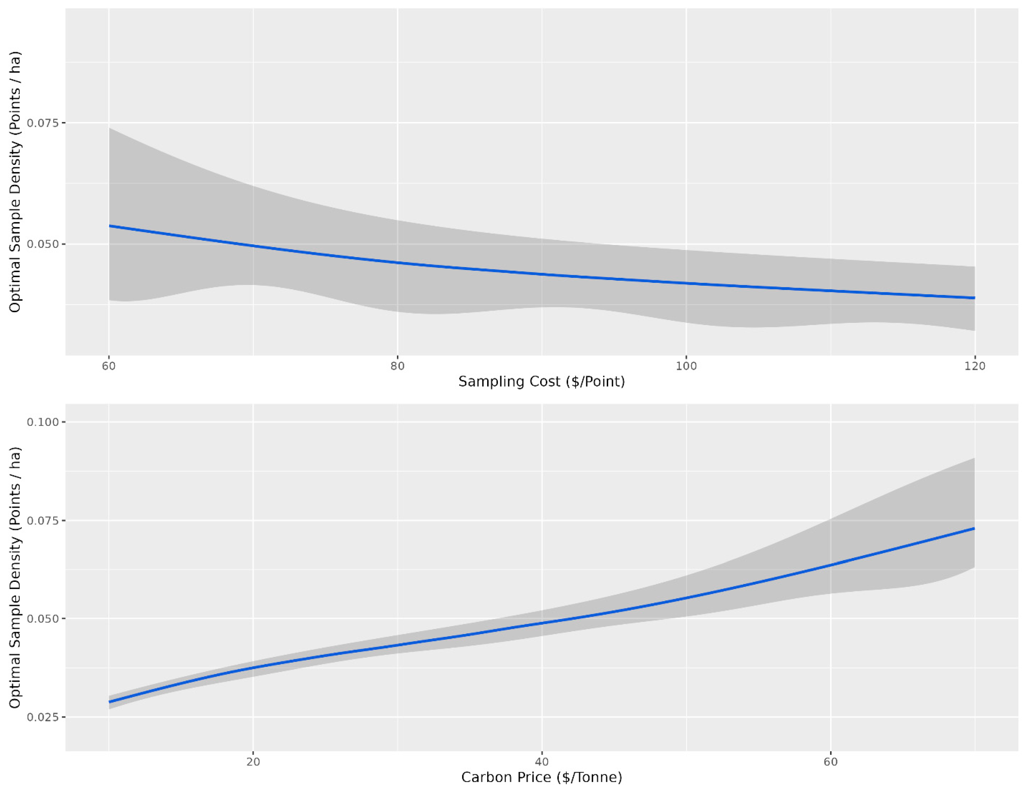
2.4. Cost–Benefit Analysis

Following the iterative predictive soil mapping model generation, the median SOC stock error was calculated for each sampling density. A nonlinear least-square model was then fit to the error as a function of the sampling density using the nls function with a self-starting biexponential model in R [51]. This was then used as part of a cost minimization function for both the conventional cLHS and the stratified cLHS sampling approaches to determine the optimal number of samples that minimized the total cost of sampling and the total cost of the carbon prediction error over the study area (Equation (1)). For this study, the total soil carbon stock error was assumed to be discounted from the final payment to the credit producer.
T o t a l   C o s t = S a m p l i n g   C o s t   ×   n + S o i l   C a r b o n   S t o c k   E r r o r   ×   C a r b o n   P r i c e   ×   T o t a l   A r e a
where
(1)
Sampling cost is the cost to obtain a soil sample;
(2)
The n parameter is the number of soil samples;
(3)
Soil carbon stock error is the soil organic carbon stock error on a Mg ha−1 basis as a function of the number of samples;
(4)
Carbon price is the price of carbon the producer receives;
(5)
Total area is the total area of interest on a hectare basis.
The number of samples needed to minimize the total cost was calculated using a range of sampling costs and carbon prices. Sampling costs were randomly generated for each run based on a normal distribution with a mean of CAD 95 per sample, with a standard deviation of CAD 10. The mean price was estimated based on an assumed cost of CAD 50 per point to collect the samples, and CAD 45 for laboratory analysis. The price of carbon for each run was randomly generated based on a normal distribution with a carbon price of CAD 30 per tonne, with a standard deviation of CAD 10. The mean price for carbon was based on Indigo Agriculture’s published carbon payment price [52]. In total, this calculation was repeated one million times for both the cLHS and the stratified cLHS. The median, 10th percentile, and 90th percentile sampling densities were then calculated based on the sampling cost and carbon price. The optimal sampling density refers to the sampling density that minimizes the sum of the total sampling cost and the SOC stock error value (Equation (1)).
An Important point to note is that detecting changes over time in a manner that avoids Type 1 and Type 2 errors is an important consideration for SOC sequestration accounting [39]. Accounting for the value of the error associated with a single point of time mapping does not capture the full costs of uncertainty. The statistical power required for confidence in detecting changes over time largely depends on the magnitude of the effect, which is heavily dependent on the time between measurement events. Therefore, this analysis should be considered a hypothetical exercise.

2.5. Analysis of Statistically Optimal Number of Points

To compare the economically optimal number of samples with the statistically optimal number of samples, the statistically optimal number of samples was determined using the methodology and R code from Saurette (2023) [53]. This methodology is based on using divergence metrics to determine an optimal number of samples to characterize the covariate space of a predictive soil mapping area, as described in Saurette et al. (2023) [32]. The clhs_min function from the opendsm package (Saurette 2023) [53] was used to calculate the statistically optimal sample sizes using 90, 95, and 99 percent confidence intervals. The covariates used were the same covariates used for the final predictive soil mapping used in this study.

3. Results and Discussion

The conventional cLHS and the stratified cLHS performed similarly based on model validation metrics (Figure 2). Generally, the performance between the two methods was similar at sampling densities below 0.15 points per ha. The stratified cLHS approach was slightly better for sampling densities of approximately 0.15 to 0.3 points per ha, and the conventional cLHS approach outperformed the stratified approach at sampling densities above 0.3. Overall, the performance between the two models was almost identical, with the GLS results indicating an increase in the R2 for the stratified cLHS of 0.002 compared to the conventional cLHS (Table 3). The R2 values for the mid-slope and the upper and crest slope positions were similar, with a maximum average R2 effect of 0.01. The differences were greater for the lower slope positions, where the stratified cLHS decreased R2 by −0.03 for lower slopes, and increased R2 by 0.05 for depressions (Table 3).
When looking at the overall average soil organic carbon stock error, the stratified cLHS had consistently lower error across sampling densities than the conventional cLHS (Figure 3). A potential explanation for the improved performance of the stratified cLHS at estimating total stocks is that SOC contents are higher in the lower slope positions (Figure 4), with the highest values occurring in the depressions. The stratified cLHS led to more accurate predictions of depression positions, which likely led to a lower overall error in the model given their importance to the overall landscape SOC stocks. Lower slope positions with higher SOC stocks have been documented by others in the Canadian Prairies, with even greater differences between crest and depressions reported than those observed in this study [54].
An explanation for the lower performance of the standard cLHS in depression positions is that cLHS aims to mimic the original distribution of the sampled population [22], thereby leading to fewer samples in landscape positions that constitute a minority of the landscape. Having few samples in lower slope positions is a concern for predictive mapping in Canadian Prairie landscapes as significant variability in soil properties can occur in lower slope positions due to differences in hydrology [55] Additionally, distributing samples evenly across feature space has been identified as important for random forest model performance [28]. Recently, feature space coverage sampling, which distributes samples more evenly across feature space, has been proposed [27]. This technique was not assessed as part of this study as it is computationally much more intensive than conventional cLHS. As 100 iterations of each sampling density were run, assessing the performance of feature space coverage sampling with this approach was not feasible given the computing resources available at the time of this study.
Overall, there were diminishing model performance returns for mapping SOC content based on the number of training sample data, with gains becoming increasingly marginal after 0.4 points per ha (Figure 3). Overall, with an average sampling cost of CAD 95 per sample and CAD 30 per tonne to the producer, the optimal sampling density for which the total cost was minimized was 0.1 points per ha for the conventional cLHS (Figure 5) and 0.04 points per ha for the stratified cLHS (Figure 6). Such a large difference between the two approaches was not expected and is likely a result of the better performance of the stratified cLHS in lower slope positions, which contain more carbon in the landscape. For a quarter section, which is the typical unit of land management in the Canadian Prairies, this corresponds to 6.5 or 2.6 points per quarter section, respectively. Note that this assumes that a quarter section is included as part of a larger mapping campaign because six or seven sample locations are not enough for predictive soil mapping with machine learning models. Further research is needed to determine the optimum minimal mapping areas for carbon stock assessment programs. This is significantly less than the optimal number of samples calculated for a 26 ha field in Ontario for which, depending on the particular criteria used, an optimal sampling density of approximately 6 points per ha has been found [32]. A likely reason for the higher density of samples in that study is the smaller area of study, compared to this project. Despite the size, a minimum number of samples is required for a PSM model, and the project scale in that study also likely involved characterizing variation at finer scales than in this study.
The optimal number of samples as a function of the price of carbon and the cost of sampling is the average given that the other variable is held constant. The confidence envelopes in Figure 5 and Figure 6 indicate the relative influence of the other variable compared to the variable of interest. Variations in the sampling cost had less influence on the optimal sampling density, ranging from just under 0.05 samples per ha at a sampling cost of CAD 60 to just over 0.025 samples at a cost of CAD 120 for stratified cLHS (Figure 6). Variations in the price of carbon had more influence on the optimal sampling density, ranging from just over 0.025 samples at CAD 10 per tonne to just under 0.075 samples at CAD 70 per tonne (Figure 3). The price of carbon had more influence, as indicated by the relatively narrower confidence envelopes.
The literature examining the optimal number of samples for predictive soil mapping is quite limited, with many studies using arbitrary approaches [23]. Typically, the number of samples collected reflects the maximum number that can be collected for a given project budget. Studies that have focused on identifying the optimal sampling densities for broad-scale mapping projects have suggested that much lower data densities can be collected than what is recommended as economically optimal in this study. This includes studies that have utilized extensive existing datasets such as the LUCAS dataset [28]. For example, a study investigating predictive soil mapping with limited sample data attempted mapping using 10 and 22 sample points (0.001 to 0.003 points per ha) for a study area of 60 km2 [29]. Another study suggested an optimal sample size of 200 to 300 samples (0.007 to 0.01 points per ha) for a 30,000 ha area [30], whereas this study would suggest on average 1200 would be needed for a 30,000 ha area.
The current published literature on selecting the optimal number of soil samples has been restricted to statistical optimization approaches. In particular, the study by Malone et al. (2019) focused on identifying the statistically optimal number of samples for a 100 ha field using cLHS and determined that the optimal sample size was 110 using the Kullbeck–Liebler distances. This corresponds to an inspection density of 1.1 samples per ha. A study in Ontario, Canada, revealed that the optimal number of points for predicting soil carbon for a 26 ha field was 146 or 154 samples, depending on whether RMSE or CCC was used for the assessment metric [32]. This corresponds to inspection densities of approximately 5.6 and 5.9 points per ha. Given that random forest models require a minimum number of samples to generalize well, the inspection densities using the methodologies in the study by Saurette et al. (2023) [32] can be hypothesized to decrease if applied to larger areas. Additionally, that study characterized variance at finer scales than this study, which may mean the sampling densities in this study were undercharacterized with subhectare variability. When determining the statistically optimal sampling density, depending on the confidence level, the mean sampling density was 0.09 points per ha for 90 percent confidence, 0.12 points per ha for 95 percent confidence, and 1819 for 99 percent confidence (Table 4). For comparison, the study sites examined here had economically optimal sampling densities ranging from approximately 0.025 to 0.075 or from 0.075 to 0.15 samples per ha depending on the sampling design methodology used. For conventional cLHS, this would mean that the economically optimal sampling density is between 90 and 95 percent confidence using the methodology from Saurette (2023) [32] depending on the price of carbon and sampling costs.

4. Conclusions

This study highlighted that the economically optimal number of samples for predictive soil mapping to support carbon stock assessments in the Canadian Prairies depended on the price of carbon and the cost of sampling. Additionally, the stratified cLHS had lower error than the conventional cLHS for a given number of sample points, likely due to better performance for depressional slope positions, which have the highest carbon stocks. Overall, attempting to characterize 99 percent of the variance in the covariate space likely will result in more samples being collected than is economically optimal. Predictive soil mapping studies should broadly consider the end use of the map, the cost associated with mapping error, and the cost to reduce that error, when determining project sample numbers. Further work is needed to determine the economically optimal number of samples without a priori soil data for an area, the minimum economically feasible mapping area, and the optimal quantity of data for detecting stock changes over time. Additionally, further work is needed to evaluate the optimal number of samples required for estimating SOC stock changes over time using bulk density data.

Supplementary Materials

The following supporting information can be downloaded at: https://www.mdpi.com/article/10.3390/land13010114/s1. Figure S1: Data processing flow diagram.

Author Contributions

Conceptualization, P.T.S.; Software, P.T.S.; Writing—original draft, P.T.S.; Writing—review & editing, J.K. and A.B.-H.; Supervision, A.B.-H. All authors have read and agreed to the published version of the manuscript.

Funding

This research was funded by Natural Sciences and Engineering Research Council grant number PDF-456429711, ALLRP 556793-20.

Data Availability Statement

The original contributions presented in the study are included in the article/Supplementary Material, further inquiries can be directed to the corresponding author.

Acknowledgments

We would like to acknowledge the Natural Sciences and Engineering Council of Canada (NSERC) for providing financial support for this project via a postdoctoral fellowship to Preston Sorenson. We acknowledge the Digital Research Alliance of Canada for providing computing resources, which were used for model training and application. We would also like to thank Hebert Grain Ventures for generously donating the soil data used for this project. Finally, this project would not have been possible without the Government of Saskatchewan and the Water Security Agency providing the LiDAR data.

Conflicts of Interest

The authors declare no conflict of interest.

References

  1. Minasny, B.; Malone, B.P.; McBratney, A.B.; Angers, D.A.; Arrouays, D.; Chambers, A.; Chaplot, V.; Chen, Z.S.; Cheng, K.; Das, B.S.; et al. Soil Carbon 4 per Mille. Geoderma 2017, 292, 59–86. [Google Scholar] [CrossRef]
  2. Liddicoat, C.; Maschmedt, D.; Clifford, D.; Searle, R.; Herrmann, T.; MacDonald, L.M.; Baldock, J. Predictive Mapping of Soil Organic Carbon Stocks in South Australia’s Agricultural Zone. Soil Res. 2015, 53, 956–973. [Google Scholar] [CrossRef]
  3. Gomes, L.C.; Faria, R.M.; de Souza, E.; Veloso, G.V.; Schaefer, C.E.G.R.; Filho, E.I.F. Modelling and Mapping Soil Organic Carbon Stocks in Brazil. Geoderma 2019, 340, 337–350. [Google Scholar] [CrossRef]
  4. Lamichhane, S.; Kumar, L.; Wilson, B. Digital Soil Mapping Algorithms and Covariates for Soil Organic Carbon Mapping and Their Implications: A Review. Geoderma 2019, 352, 395–413. [Google Scholar] [CrossRef]
  5. Bartholomeus, H.; Kooistra, L.; Stevens, A.; van Leeuwen, M.; van Wesemael, B.; Ben-Dor, E.; Tychon, B. Soil Organic Carbon Mapping of Partially Vegetated Agricultural Fields with Imaging Spectroscopy. Int. J. Appl. Earth Obs. Geoinf. 2011, 13, 81–88. [Google Scholar] [CrossRef]
  6. Wang, S.; Zhuang, Q.; Wang, Q.; Jin, X.; Han, C. Mapping Stocks of Soil Organic Carbon and Soil Total Nitrogen in Liaoning Province of China. Geoderma 2017, 305, 250–263. [Google Scholar] [CrossRef]
  7. Sothe, C.; Gonsamo, A.; Arabian, J.; Snider, J. Large Scale Mapping of Soil Organic Carbon Concentration with 3D Machine Learning and Satellite Observations. Geoderma 2022, 405, 115402. [Google Scholar] [CrossRef]
  8. Black, C.; Brummit, C.; Campbell, N.; DuBuisson, M.; Harburg, D.; Matosziuk, L.; Motew, M.; Pinjuv, G.; Smith, E. Methodology for Improved Agricultural Land Management. 2023. Available online: https://verra.org/methodologies/vm0042-methodology-for-improved-agricultural-land-management-v2-0/ (accessed on 19 January 2024).
  9. McBratney, A.B.; Mendonça Santos, M.L.; Minasny, B. On Digital Soil Mapping. Geoderma 2003, 117, 3–52. [Google Scholar] [CrossRef]
  10. Mulder, V.L.; de Bruin, S.; Schaepman, M.E.; Mayr, T.R. The Use of Remote Sensing in Soil and Terrain Mapping—A Review. Geoderma 2011, 162, 1–19. [Google Scholar] [CrossRef]
  11. Dobos, E.; Micheli, E.; Baumgardner, M.F.; Biehl, L.; Helt, T. Use of Combined Digital Elevation Model and Satellite Radiometric Data for Regional Soil Mapping. Geoderma 2000, 97, 367–391. [Google Scholar] [CrossRef]
  12. Hengl, T.; Leenaars, J.G.B.; Shepherd, K.D.; Walsh, M.G.; Heuvelink, G.B.M.; Mamo, T.; Tilahun, H.; Berkhout, E.; Cooper, M.; Fegraus, E.; et al. Soil Nutrient Maps of Sub-Saharan Africa: Assessment of Soil Nutrient Content at 250 m Spatial Resolution Using Machine Learning. Nutr. Cycl. Agroecosyst. 2017, 109, 77–102. [Google Scholar] [CrossRef] [PubMed]
  13. Guevara, M.; Arroyo, C.; Brunsell, N.; Cruz, C.O.; Domke, G.; Equihua, J.; Etchevers, J.; Hayes, D.; Hengl, T.; Ibelles, A.; et al. Soil Organic Carbon Across Mexico and the Conterminous United States (1991–2010). Glob. Biogeochem. Cycles 2020, 34, e2019GB006219. [Google Scholar] [CrossRef]
  14. Hengl, T.; Mendes de Jesus, J.; Heuvelink, G.B.M.; Ruiperez Gonzalez, M.; Kilibarda, M.; Blagotić, A.; Shangguan, W.; Wright, M.N.; Geng, X.; Bauer-Marschallinger, B.; et al. SoilGrids250m: Global Gridded Soil Information Based on Machine Learning. PLoS ONE 2017, 12, e0169748. [Google Scholar] [CrossRef] [PubMed]
  15. Lacoste, M.; Mulder, V.L.; Saby, N.; Arrouays, D. High-Resolution Spatial Modelling of Total Soil Depth for France. Available online: https://www.researchgate.net/profile/Vl-Mulder/publication/269400505_High-resolution_spatial_modelling_of_total_soil_depth_for_France/links/5489ac0c0cf2d1800d7a9da3/High-resolution-spatial-modelling-of-total-soil-depth-for-France.pdf (accessed on 30 October 2023).
  16. Heung, B.; Bulmer, C.E.; Schmidt, M.G. Predictive Soil Parent Material Mapping at a Regional-Scale: A Random Forest Approach. Geoderma 2014, 214–215, 141–154. [Google Scholar] [CrossRef]
  17. Kasraei, B.; Heung, B.; Saurette, D.D.; Schmidt, M.G.; Bulmer, C.E.; Bethel, W. Quantile Regression as a Generic Approach for Estimating Uncertainty of Digital Soil Maps Produced from Machine-Learning. Environ. Model. Softw. 2021, 144, 105139. [Google Scholar] [CrossRef]
  18. Fathololoumi, S.; Vaezi, A.R.; Alavipanah, S.K.; Ghorbani, A.; Saurette, D.; Biswas, A. Improved Digital Soil Mapping with Multitemporal Remotely Sensed Satellite Data Fusion: A Case Study in Iran. Sci. Total Environ. 2020, 721, 137703. [Google Scholar] [CrossRef]
  19. Wadoux, A.M.J.C.; Minasny, B.; McBratney, A.B. Machine Learning for Digital Soil Mapping: Applications, Challenges and Suggested Solutions. Earth Sci. Rev. 2020, 210, 103359. [Google Scholar] [CrossRef]
  20. Pennock, D.J. Designing Field Studies in Soil Science. Can. J. Soil Sci. 2004, 84, 1–10. [Google Scholar] [CrossRef]
  21. Biswas, A.; Zhang, Y. Sampling Designs for Validating Digital Soil Maps: A Review. Pedosphere 2018, 28, 1–15. [Google Scholar] [CrossRef]
  22. Minasny, B.; McBratney, A.B. A Conditioned Latin Hypercube Method for Sampling in the Presence of Ancillary Information. Comput. Geosci. 2006, 32, 1378–1388. [Google Scholar] [CrossRef]
  23. Malone, B.P.; Minansy, B.; Brungard, C. Some Methods to Improve the Utility of Conditioned Latin Hypercube Sampling. PeerJ 2019, 7, e6451. [Google Scholar] [CrossRef]
  24. Saurette, D.D.; Biswas, A.; Heck, R.J.; Gillespie, A.W.; Berg, A.A. Determining Minimum Sample Size for the Conditioned Latin Hypercube Sampling Algorithm. Pedosphere 2022. in press. [Google Scholar] [CrossRef]
  25. Yang, L.; Li, X.; Shi, J.; Shen, F.; Qi, F.; Gao, B.; Chen, Z.; Zhu, A.X.; Zhou, C. Evaluation of Conditioned Latin Hypercube Sampling for Soil Mapping Based on a Machine Learning Method. Geoderma 2020, 369, 114337. [Google Scholar] [CrossRef]
  26. Godinho Silva, S.H.; Owens, P.R.; Silva, B.M.; César de Oliveira, G.; Duarte de Menezes, M.; Pinto, L.C.; Curi, N. Evaluation of Conditioned Latin Hypercube Sampling as a Support for Soil Mapping and Spatial Variability of Soil Properties. Soil Sci. Soc. Am. J. 2015, 79, 603–611. [Google Scholar] [CrossRef]
  27. Ma, T.; Brus, D.J.; Zhu, A.-X.; Zhang, L.; Scholten, T. Comparison of Conditioned Latin Hypercube and Feature Space Coverage Sampling for Predicting Soil Classes Using Simulation from Soil Maps. Geoderma 2020, 370, 114366. [Google Scholar] [CrossRef]
  28. Wadoux, A.M.J.C.; Brus, D.J.; Heuvelink, G.B.M. Sampling Design Optimization for Soil Mapping with Random Forest. Geoderma 2019, 355, 113913. [Google Scholar] [CrossRef]
  29. Zhu, A.X.; Liu, J.; Du, F.; Zhang, S.J.; Qin, C.Z.; Burt, J.; Behrens, T.; Scholten, T. Predictive Soil Mapping with Limited Sample Data. Eur. J. Soil Sci. 2015, 66, 535–547. [Google Scholar] [CrossRef]
  30. Titia, V.L. Digital Soil Mapping; Boettinger, J.L., Howell, D.W., Moore, A.C., Hartemink, A.E., Kienast-Brown, S., Eds.; Springer: Dordrecht, The Netherlands, 2010; ISBN 978-90-481-8862-8. [Google Scholar]
  31. Stumpf, F.; Schmidt, K.; Behrens, T.; Schönbrodt-Stitt, S.; Buzzo, G.; Dumperth, C.; Wadoux, A.; Xiang, W.; Scholten, T.; Schönbrodt-Stitt, S.; et al. Incorporating Limited Field Operability and Legacy Soil Samples in a Hypercube Sampling Design for Digital Soil Mapping. J. Plant Nutr. Soil Sci. 2016, 179, 499–509. [Google Scholar] [CrossRef]
  32. Saurette, D.D.; Heck, R.J.; Gillespie, A.W.; Berg, A.A.; Biswas, A. Divergence Metrics for Determining Optimal Training Sample Size in Digital Soil Mapping. Geoderma 2023, 436, 116553. [Google Scholar] [CrossRef]
  33. Kollmuss, A.; Lazarus, M. Discounting Offsets: Issues and Options. Carbon Manag. 2011, 2, 539–549. [Google Scholar] [CrossRef]
  34. SKSIS Working Group Saskatchewan Soil Information System–SKSIS. Available online: https://soilsofsask.ca/saskatchewan-soil-information-system.php (accessed on 2 May 2021).
  35. LaZerte, S.E.; Albers, S. Weathercan: Download and Format Weather Data from Environment and Climate Change Canada. J. Open Source Softw. 2018, 3, 571. [Google Scholar] [CrossRef]
  36. Kiss, J.; Bedard-Haughn, A.; Sorenson, P. Predictive Mapping of Wetland Soil Types in the Canadian Prairie Pothole Region Using High-Resolution Digital Elevation Model Terrain Derivatives. Can. J. Soil Sci. 2022, 103, 21–46. [Google Scholar] [CrossRef]
  37. Carter, M.R.; Gregorich, E.G. (Eds.) Soil Sampling and Methods of Analysis; CRC Press: Boca Raton, FL, USA, 2007; ISBN 9780429126222. [Google Scholar]
  38. Agriculture and Agri-Food Canada National Pedon Database. Available online: https://open.canada.ca/data/en/dataset/6457fad6-b6f5-47a3-9bd1-ad14aea4b9e0 (accessed on 16 February 2021).
  39. Stanley, P.; Spertus, J.; Chiartas, J.; Stark, P.B.; Bowles, T. Valid Inferences about Soil Carbon in Heterogeneous Landscapes. Geoderma 2023, 430, 116323. [Google Scholar] [CrossRef]
  40. Roudier, P. Clhs: A R Package for Conditioned Latin Hypercube Sampling. 2011. Available online: https://cran.r-project.org/web/packages/clhs/clhs.pdf (accessed on 30 October 2023).
  41. Boehner, J.; Selige, T. Spatial Prediction of Soil Attributes Using Terrain Analysis and Climate Regionalisation. In SAGA–Analyses and Modelling Applications; Boehner, J., McCloy, K.R., Strobl, J., Eds.; Göttinger Geographische Abhandlungen; Universität Göttingen: Göttingen, Germany, 2006; pp. 13–27. [Google Scholar]
  42. Brenning, A.; Bangs, D.; Becker, M. RSAGA: SAGA Geoprocessing and Terrain Analysis. 2018. Available online: https://cran.r-project.org/web/packages/RSAGA/index.html (accessed on 30 October 2023).
  43. Gorelick, N.; Hancher, M.; Dixon, M.; Ilyushchenko, S.; Thau, D.; Moore, R. Google Earth Engine: Planetary-Scale Geospatial Analysis for Everyone. Remote Sens. Environ. 2017, 202, 18–27. [Google Scholar] [CrossRef]
  44. Sorenson, P.T.; Shirtliffe, S.J.; Bedard-Haughn, A.K. Predictive Soil Mapping Using Historic Bare Soil Composite Imagery and Legacy Soil Survey Data. Geoderma 2021, 401, 115316. [Google Scholar] [CrossRef]
  45. Gallant, J.C.; Dowling, T.I. A Multiresolution Index of Valley Bottom Flatness for Mapping Depositional Areas. Water Resour. Res. 2003, 39, 1347. [Google Scholar] [CrossRef]
  46. Sorenson, P. Google Earth Engine Scripts for Generating Predictive Soil Mapping Environmental Covariates. Available online: https://github.com/prestonsorenson/Google_Earth_Engine_PSM/tree/main (accessed on 15 August 2021).
  47. Stevens, A.; Ramirez-Lopez, L. An Introduction to the Prospectr Package. 2014. Available online: https://cran.r-project.org/web/packages/prospectr/vignettes/prospectr.html (accessed on 30 October 2023).
  48. Sorenson, P.T.; Kiss, J.; Serdetchnaia, A.; Iqbal, J.; Bedard-Haughn, A.K. Predictive Soil Mapping in the Boreal Plains of Northern Alberta by Using Multi-Temporal Remote Sensing Data and Terrain Derivatives. Can. J. Soil Sci. 2022, 102, 852–866. [Google Scholar] [CrossRef]
  49. Wright, M.N.; Ziegler, A. Ranger: A Fast Implementation of Random Forests for High Dimensional Data in C++ and R. J. Stat. Softw. 2017, 77, 1–17. [Google Scholar] [CrossRef]
  50. Pinheiro, J.; Bates, D. nlme: Linear and Nonlinear Mixed Effects Models. 2022. Available online: https://cran.r-project.org/web/packages/nlme/nlme.pdf (accessed on 30 October 2023).
  51. R Core Team R: A Language and Environment for Statistical Computing. 2018. Available online: https://www.gbif.org/tool/81287/r-a-language-and-environment-for-statistical-computing (accessed on 30 October 2023).
  52. Indigo Agriculture. Carbon by Indigo Farmers Receive Second Carbon Farming Payment. Available online: https://www.indigoag.com/pages/news/carbon-by-indigo-farmers-receive-second-carbon-farming-payment (accessed on 30 October 2023).
  53. Saurette, D. Opendsm. Available online: https://github.com/newdale/opendsm (accessed on 18 December 2023).
  54. Landi, A.; Mermut, A.R.; Anderson, D.W. Carbon Distribution in a Hummocky Landscape from Saskatchewan, Canada. Soil Sci. Soc. Am. J. 2004, 68, 175–184. [Google Scholar] [CrossRef]
  55. Pennock, D.; Bedard-Haughn, A.; Kiss, J.; van der Kamp, G. Application of Hydropedology to Predictive Mapping of Wetland Soils in the Canadian Prairie Pothole Region. Geoderma 2014, 235–236, 199–211. [Google Scholar] [CrossRef]
Figure 1. Overview map indicating the location of the study. All soil samples were collected within the areas indicated with the red squares. The dashed black line is the provincial boundary for the province of Saskatchewan. The red squares indicate the specific study areas. The base map is the median Landsat 7 2000 to 2020 May-to-October median surface reflectance. The coordinates are in UTM Zone 13N (EPSG: 26913).
Land 13 00114 g001
Figure 2. R2, CCC, relative error, and root-mean-square error for conventional and landscape-stratified conditioned Latin hypercube sampling by the number of sampling points. Locally estimated scatter plot smoothing results for conventional and landscape stratified are presented. The confidence intervals, represented by the shaded areas, for each graph correspond to the 10th and 90th percentile values.
Land 13 00114 g002
Figure 3. Average soil organic carbon stock error for conventional and landscape stratified conditioned Latin hypercube sample designs as a function of the number of sample points. The error is determined based on the total carbon stock for each sampling design compared to when the entire dataset is used for the entire study area.
Land 13 00114 g003
Figure 4. Soil organic carbon concentrations across slope positions within the study area.
Land 13 00114 g004
Figure 5. Optimal sampling density for the conventional conditioned Latin hypercube sampling design based on the cost of sampling and the price of carbon. The shaded grey ribbon corresponds to the 10th and 90th percentile sampling densities for a given sampling density (points ha−1). For the top panel, the optimal sampling density is presented as a function of sampling cost, and for the bottom panel, the optimal sampling density is presented as a function of the price of carbon. The grey confidence intervals indicate the variability in optimal sampling density based on variability in carbon price for the top panel and sampling cost for the bottom panel.
Land 13 00114 g005
Figure 6. Optimal sampling density for the landscape stratified conditioned Latin hypercube sampling design based on the cost of sampling and the price of carbon. The shaded grey ribbon corresponds to the 10th and 90th percentile sampling densities for a given sampling density (points ha−1). For the top panel, the optimal sampling density is presented as a function of sampling cost, and for the bottom panel, the optimal sampling density is presented as a function of the price of carbon. The grey confidence intervals indicate the variability in optimal sampling density based on variability in carbon price for the top panel and sampling cost for the bottom panel.
Land 13 00114 g006
Table 1. Soil organic carbon values.
ParameterMin25th PercentileMedian75th PercentileMax
Soil organic carbon (%)0.642.092.492.963.71
MeanStandard DeviationCoefficient of VariationKurtosisSkewness
2.520.590.232.44−0.01
Table 2. Remote sensing variables.
FeatureDate
Sentinel-2 bare soil composite imagery
● Band 8 (near infrared)
● Band 11 (shortwave infrared 1)
● Band 12 (shortwave infrared 2)
Median of bare soil pixels from April to October from 2017 to 2022.
Sentinel-2 imagery
● Band 2 (blue)
● Band 3 (green)
● Band 4 (red)
● Band 5 (red edge 1)
● Band 6 (red edge 2)
● Band 7 (red edge 3)
● Band 8 (near infrared)
● Band 8a (red edge 4)
● Band 11 (shortwave infrared 1)
● Band 12 (shortwave infrared 2)
Median of pixels from May to October from 2017 to 2022.
Normalized difference vegetation index derived from Sentinel-2 imagery
● May-to-October NDVI
● May NDVI
● June NDVI
● July NDVI
● August NDVI
● September NDVI
● October NDVI
● Max NDVI minus minimum NDVI
● Standard deviation of NDVI
Median of pixels from May to October from 2017 to 2022.
Sentinel-1 Data
● Vertical–vertical polarization (VV)
● Vertical–horizontal polarization (VH)
● Normalized difference of VV and VH polarizations
Median of pixels from May to October from 2017 to 2022.
Terrain attributes
● Normalized height [41]
● Slope height [41]
● Saga wetness index [41]
● Multiresolution ridge top flatness index [45]
● Multiresolution valley bottom flatness [45]
● Plan curvature
● Profile curvature
Derived from light detection and ranging digital elevation model. The original DEM resolution was 0.5 m, and it was resampled to 5 m.
Table 3. Generalized least-square model results comparing R2 between conventional and stratified conditioned Latin hypercube sampling (cLHS) designs with the number of points as a first-order autocorrelation structure. The results for the conventional cLHS are embedded in the intercept term, and the stratified term indicates the difference compared to the conventional cLHS.
Slope Position ValueStandard Errort-Valuep-Value
OverallIntercept0.370.0008459.63<0.01
Type: Stratified0.0020.00053.39<0.01
DepressionIntercept0.270.0003678.68<0.01
Type: Stratified0.050.000592.10<0.01
Lower slopeIntercept0.240.0008277.14<0.01
Type: Stratified−0.030.001−24.45<0.01
Mid-slopeIntercept0.300.0005565.07<0.01
Type: Stratified0.0040.00066.56<0.01
Upper slopeIntercept0.350.0005693.31<0.01
Type: Stratified−0.0040.006−7.37<0.01
CrestIntercept0.440.0008535.06<0.01
Type: Stratified−0.010.0009−9.88<0.01
Table 4. The statistically optimal number of samples and sample densities to characterize the covariate space at 90, 95, and 99 percent confidence.
Percent ConfidenceMinimum (Samples/Density)Mean (Samples/Density)Median (Samples/Density)Maximum (Samples/Density)Standard Deviation (Samples/Density)
9092/0.02438/0.09327/0.071089/0.23287/0.06
9592/0.02578/0.12428/0.091783/0.37425/0.09
9992/0.021819/0.38695/0.1513151/2.802821/0.60
Disclaimer/Publisher’s Note: The statements, opinions and data contained in all publications are solely those of the individual author(s) and contributor(s) and not of MDPI and/or the editor(s). MDPI and/or the editor(s) disclaim responsibility for any injury to people or property resulting from any ideas, methods, instructions or products referred to in the content.

