Article

U-Net-STN: A Novel End-to-End Lake Boundary Prediction Model

1
Department of Geography & Anthropology, Louisiana State University, Baton Rouge, LA 70803, USA
2
School of Automation, University of Electronic Science and Technology of China, Chengdu 610054, China
3
College of Resource and Environment Engineering, Guizhou University, Guiyang 550025, China
4
School of Public Affairs and Administration, University of Electronic Science and Technology of China, Chengdu 611731, China
5
School of Geographical Sciences, Southwest University, Chongqing 400715, China
*
Author to whom correspondence should be addressed.
Land 2023, 12(8), 1602; https://doi.org/10.3390/land12081602
Submission received: 25 July 2023 / Revised: 11 August 2023 / Accepted: 13 August 2023 / Published: 14 August 2023
(This article belongs to the Special Issue Assessment of Land Use/Cover Change Using Geospatial Technology)

Abstract

:
Detecting changes in land cover is a critical task in remote sensing image interpretation, with particular significance placed on accurately determining the boundaries of lakes. Lake boundaries are closely tied to land resources, and any alterations can have substantial implications for the surrounding environment and ecosystem. This paper introduces an innovative end-to-end model that combines U-Net and spatial transformation network (STN) to predict changes in lake boundaries and investigate the evolution of the Lake Urmia boundary. The proposed approach involves pre-processing annual panoramic remote sensing images of Lake Urmia, obtained from 1996 to 2014 through Google Earth Pro Version 7.3 software, using image segmentation and grayscale filling techniques. The results of the experiments demonstrate the model’s ability to accurately forecast the evolution of lake boundaries in remote sensing images. Additionally, the model exhibits a high degree of adaptability, effectively learning and adjusting to changing patterns over time. The study also evaluates the influence of varying time series lengths on prediction accuracy and reveals that longer time series provide a larger number of samples, resulting in more precise predictions. The maximum achieved accuracy reaches 89.3%. The findings and methodologies presented in this study offer valuable insights into the utilization of deep learning techniques for investigating and managing lake boundary changes, thereby contributing to the effective management and conservation of this significant ecosystem.

1. Introduction

Changes in the Earth’s surface cover and its man-made development have caused various impacts on ecosystems and environmental processes on a local, regional, and global scale [1,2,3]. The detection of lake boundaries is extremely important for predicting future lake boundary changes and supporting future lake protection policy decisions [4]. By studying changes in the lake boundary, it is possible to monitor the impact of various factors on the lake. This information helps assess the ecological integrity of the lake and identify any potential threats and is critical for the effective management and conservation of freshwater resources [5,6,7]. Remote sensing has become the main source of lake spatial information [8,9], and remote sensing images intuitively show the spatial distribution and dynamic change process of natural lakes. Remote sensing data reduce the manual work of collecting data on-site and reduce the cost of obtaining geographic information [10,11]. With the development of remote sensing technology and digital image processing technology, computer-based remote sensing image processing has recently become popular [12,13]. People began to study the characteristics of lake boundary changes extracted from remote sensing images in different periods and, based on this, predict the future changes in lake boundaries.
Traditional methods of lake boundary feature extraction from remote sensing images mainly include digital terrain models (DTM) [14], semantic segmentation [15,16], and object-oriented methods [17]. In 2003, Jiang L. et al. [18] proposed a shape-based time-series remote sensing image lake change detection method. They use supervised classification, object recognition, parametric contour tracking, and a proposed piecewise linear polygon approximation technique to represent feature shapes in remote sensing images. In 2020, Julzarika [19] tested the effectiveness of DTM in Lake Oduli on the island of Rote. Julzarika used both digital elevation models (DEM), DTM, and digital surface models (DSM). Among them, DEM includes both Sentinel and Planet images. The DSM is an integration of the DEM. However, DTM is obtained from the derivative result of DSM. However, the experimental results show that the DTM has a 95% error rate in predicting the lake boundary of Lake Oduli. This may be caused by the poor recognition of impurities in the lake by DTM. The traditional method of lake boundary extraction using semantic segmentation often has problems with over-segmentation and inaccurate segmentation. In order to solve these problems, in 2020, Zhong et al. [15] designed an end-to-end semantic segmentation network, the noise cancellation transformer network (NT-Net), by improving the semantic segmentation network using transform. To solve the problems of over-segmentation and inaccurate segmentation, the interference attenuation module and the multi-stage transformer module are introduced into NT-Net, respectively. The interference attenuation module can suppress the feature representations of non-lake objects by analyzing the differences between the feature representations of lakes and other ground objects to model the key features that are distinguishable and suitable for lake water segmentation. The multi-stage transformer module can capture the contextual association of boundary information and enhance the feature representation of boundary information by using the self-attention mechanism.
Nowadays, with the development of artificial intelligence, more and more researchers use deep learning [20,21,22] to complete the extraction of lake boundary features and predict the lake boundary according to its changing characteristics. Compared with traditional methods, deep learning models, with their ability to automatically extract features and superior computing power, have great potential to become valuable tools for analyzing and predicting lake boundary changes [23]. CNN has been widely used in image processing fields such as object positioning, object recognition, target segmentation, key point detection, and so on [24,25,26]. However, CNN and other deep learning models are not so effective in remote sensing change detection for lake boundary change prediction. Some studies first use CNN and other depth learning models for remote sensing image fusion [27,28], image registration [29], and image semantic segmentation [30], and then detect the change in the processed remote sensing image. Other research directly extracts change features using a deep learning model, and then they produce a change difference map using the retrieved change features [31,32]. This research terminates at change detection and can only manually visually assess historical surface cover data to determine the general change trend of the lake boundary.
All these methods mentioned above use remote sensing images to extract the characteristics of a lake boundary change, analyze the trend of lake boundary change based on these characteristics, and then make predictions. In fact, these methods include two parts: change trend analysis and change prediction, and the operation steps are more cumbersome. To effectively solve the above problems, this paper proposes a novel end-to-end prediction network based on the dynamic evolution of the lake boundary in remote sensing images. The network combined the U-Net model improved from CNN and the spatial transformation network (STN) [33], which retained the spatial structure and context information of each pixel in the image, making it possible to complete feature extraction and change prediction in one network at the same time. Firstly, U-Net processes a pair of consecutive images in the time series image, extracts the changes between the before and after images, and fits the corresponding evolution field. STN then predicts the change in surface coverage based on the resulting evolution field. Taking Lake Urmia as a case, this study performs image segmentation and image grayscale filling pre-processing operations on small sensing images in some areas of panoramic remote sensing images of Lake Urmia and then inputs them into the model designed in this paper for prediction.

2. Dataset and Pre-Processing

2.1. Study Area

Lake Urmia is the largest lake in Iran, located in the basin between the provinces of East Azerbaijan and West Azerbaijan in the northwest of Iran, and is the second largest saltwater lake on earth, as shown in Figure 1. The lake once covered an area of 5200 square kilometers and was 16 m deep. Environmental changes have caused a 70% reduction in the surface area of Lake Urmia between 2002 and 2016. The ecological environment has undergone tremendous changes, the salinity of the lake water has increased, and the number of migratory birds and organisms in the lake has decreased.

2.2. Dataset

According to the research objectives, this paper selects two datasets for experiments. The data used are satellite image data obtained from Google Earth Pro software. The first dataset is the panoramic remote sensing image of Lake Urmia to verify the effectiveness of this model in predicting the overall evolution trend of cover; the second dataset is the remote sensing images of some areas of Lake Urmia to test the ability of this model to capture regional details.

2.2.1. Dataset 1: Sequence of Panoramic Historical Images of Lake Urmia

In this study, the historical images of the Google Earth remote sensing satellite of Lake Urmia from 1996 to 2014 are arranged in chronological order to form the first time series dataset, with 19 scenes. Each scene is taken on 30 December of that year, and the image size is 560 × 640. Latitudes are taken from 37°00′ N to 38°15′ N and longitudes from 46°10′ E to 44°50′ E, as shown in Figure 2. This is abbreviated as dataset 1.
The data from 1996 to 2013 are mainly used as the data source for surface cover prediction, and the training set and test set are selected from them, while the 2014 image is not used for training, and is mainly used to test the predictive generalization ability of the trained model. During training, the model uses N images of the next year to predict its surface cover map in the next year, and the corresponding image of this year in the dataset is used as the ground truth. For example, the CNN prediction model used 1999 and 2000 images as input for training, the model learned the law of cover evolution and predicted its cover map in 2001, and the data in 2001 in the dataset are used as the ground truth to calculate loss.

2.2.2. Dataset 2: Sequence of Partial Historical Images of Lake Urmia

This section selects the historical images of the Google Earth remote sensing satellite in the north part of Lake Urmia from 2000 to 2014 to form the second time series dataset. Latitudes are taken from 38°05′ N to 38°15′ N and longitudes from 45°30′ E to 44°20′ E. The size of a single image is 1280 × 560 , taking the year as the cycle unit, there are 15 scenes in total, and each scene is taken on 30 December of that year, as shown in Figure 3. This is abbreviated as dataset 2.
Among them, the data from 2000–2013 are mainly used as the data source for surface cover prediction, and the training set and test set are selected from them, while the 2014 image is not used for training and is mainly used to test the predictive generalization ability of the trained model. For example, the U-Net prediction model used 2008 and 2009 images as input, the model learned the law of cover evolution and predicted its cover map in 2010, and the data in the dataset for 2010 are used as ground truth to calculate loss.

2.3. Pre-Processing

2.3.1. Image Segmentation

Image segmentation and binarization are essential pre-processing steps for remote sensing images [34,35]. In remote sensing, image segmentation is useful for separating different land cover types. By segmenting the image, it is easier to extract information from each segment, and it can also help reduce the computational cost of processing large images. In remote sensing, binarization is often used to separate the land cover from the background and to identify specific features of interest. This process can also help to reduce the complexity of the image and make it easier to analyze.
First, 15 remote sensing images were separated to distinguish the lake area from other areas. Image segmentation is conducive to the visualization of the evolution process of the lake boundary and is of great help to the follow-up model to learn the evolution process of the overburden layer. Figure 4 shows the results of remote sensing image segmentation and binarization in 2000.

2.3.2. Image Grayscale Gradient Fill

The gray gradient filling method mainly includes three steps:
In the first step, the coating boundary in the image gradually shrinks smoothly to the coating center through multiple continuous erosion operations, and the intermediate results after each shrinkage are saved. Image boundary erosion processing involves removing the edges of an image to reduce the impact of edge artifacts [36]. The erosion algorithm of image A using erosion operator B can be expressed as Equation (1).
A   B = z ( B ) z A ,
The erosion operator B is a circular operator with a radius of 3.
For erosion operation , use erosion operator B to corrode binary image A once. The flow of erosion once is shown in Algorithm 1.
Algorithm 1: Erosion Algorithm
Input: Binary image A , erosion operator B Output: Erosion results A B
  • Select the category, size, and center point z of the erosion operator B .
  • Select the area A to be corroded of the original image A , and the remaining area is denoted as A A , and the pixels set of A is denoted as N ( p ) .
  • Make the center point z of B coincide with an unselected point p in N ( p ) , and then coincide other pixels of B with the corresponding pixel of A .
  • Select an unselected point m with a pixel value of 1 in B , and find the corresponding pixel m in A that coincides with it. If the pixel value of m is 0, delete the point ( p ) in N p , that is, the pixel value of point p is 0. Otherwise, continue to select another point m with a pixel value of 1 in B and repeat step 4 until all the pixels in B are traversed.
  • Repeat steps 3–4 until N ( p ) was traversed.
  • Combine the updated N ( p ) with A A , and get erosion results A B .
The erosion operator is also called a structural element. Generally, cross, rectangle, circle, and ellipse can be selected. This paper uses a circular operator with a radius of 3 to sequentially corrode the 2000 images in the second dataset 50 times. Some of the results are shown in Figure 5.
In the second step, the difference image of two adjacent shrinkage images is obtained by subtracting in sequence according to the erosion order. The pixel value corresponding to the i + 1 erosion result is subtracted from the i + 1 erosion result. The point set with a difference of 255 is the pixel point set deleted during the i + 1 erosion, and the result is displayed as the lake boundary. Figure 6 shows a partial difference image after the erosion of the binarization image of Lake Urmia in 2000.
The third step is to sort the obtained difference image set in turn, fill the gray level from front to back according to the linear change, and change the pixel value of the white points in the difference image. Filling the lakes in the segmented binarized image with grayscale gradients can add additional contextual information to the image [37].
The gray value of the pixel set in the first difference image is the highest, close to white, and the gray value of the pixel set in the last difference image is the lowest, close to black. The erosion times are 50, the gray value of the outermost boundary is the highest, which is 200, and the gray level series is 2. Therefore, the gray value of the innermost layer is the lowest, which is 100. The erosion times, gray level series, and the highest gray value can be selected according to the size of the remote sensing image. The algorithm flow is shown in Algorithm 2.
Algorithm 2: Grayscale Gradient Fill Algorithm
Input: Binarized image A Output: Grayscale fill image A
  • Let P = A , i = 1 , α = N u m b e r   o f   e r o s i o n s , G m a x = The highest gray value, G = G m a x , l = G r a y s c a l e   p r o g r e s s i o n , G m a x < 255   G m i n = G m a x l × α > 0 .
  • According to algorithm 1: the i-th erosion operation was performed to P , and the obtained result is Q .
  • Let R i = P Q , that is, the corresponding pixel values are subtracted, and the difference image is R i , and the set of points with a difference of 255 is denoted as N ( p ) .
  • Set all pixels belonging to N ( p ) in the image. R i to have pixel values G .
  • Let P = Q , G = G m a x l × i , i = i + 1 . If i α , repeat steps 2–5. Otherwise, proceed to step 6.
  • Let A = R 1 + R 2 + + R 49 + R 50 , that is, the corresponding pixel values of 50 differential images R i are added together to obtain a grayscale gradient-filled image A .

2.3.3. Wave Filtering

After the image filled with a gray gradient is filtered, the gray change tends to be smooth. It is beneficial to the subsequent gradient descent algorithm of the model to obtain the optimal solution [38].
The filtering algorithm uses Gaussian filtering, and Equation (2) is a two-dimensional Gaussian function for calculating the weights of neighboring pixels. The size of the Gaussian kernel is 5 × 5.
G x , y = 1 2 π σ 2 e ( x 2 + y 2 ) / 2 σ 2 ,

3. Method

The dynamic evolution prediction algorithm flow of the remote sensing image lake boundary designed in this study is shown in Figure 7. It can be roughly divided into five steps: image pair pre-processing, evolution feature extraction, feature fusion, spatial transformation, and coverage prediction.
(1)
Image pair pre-processing. Input two remote sensing images that were taken every other year. The pre-processing methods are used for cover segmentation, image binarization, erosion, difference, gray gradient filling, and filtering for subsequent evolutionary feature extraction;
(2)
Evolutionary feature extraction. Input the pre-processed image pair in step (1), increase the dimension of the input image, and then splice the image pair along the increased dimension. The input feature extraction module is composed of multiple convolution layers with the same convolution kernel size to extract the multi-scale features of the input image pair;
(3)
Feature fusion. The features extracted in the previous step are decoded through the multi-layer upper sampling layer, and the decoded features are fused with the multi-scale features of the same size extracted in step (2), which are input into the subsequent layer to learn and obtain the evolution field required for prediction;
(4)
Spatial transformation. Using the evolution field learned in the previous module, the corresponding spatial transformation operation is performed on the subsequent time series image y of the input image pairy, and the image obtained after spatial transformation is the predicted land cover map z _ p r e d of the next time series target area;
(5)
Cover prediction. Enter ground truth, i.e., the next sequential image z of y , compare the output z _ p r e d of step (4), calculate to obtain the loss, and train the parameters of the network with the backpropagation.
The specific content is introduced in detail below.

3.1. Evolutionary Feature Extraction and Fusion Module

Different from the traditional change detection methods, the use of a change map can only show the characteristics of the limited target area. This model uses a CNN model similar to the U-Net [39] structure to fit the change mapping between two temporal remote sensing images and retains the position spatial structure and context information of each pixel in the image. U-Net is a CNN architecture designed for semantic segmentation tasks. The U-Net architecture has skip connections connecting the encoder and decoder layers at multiple resolutions. These connections enable the decoder to access low-level and high-level features, which help preserve spatial details and improve segmentation accuracy. The model structure is shown in Figure 8.
One specific network structure is used in this experiment, but other network frameworks and structures may also be applicable. The same number of network layers and convolution kernel parameters are not our requirements. The change mapping modeling between image pairs fitted by the U-Net model is expressed as Equation (3):
g θ x , y = φ ,
Among them, x , y are two temporal remote sensing images, φ is the evolution field fitting the displacement of each pixel of x , y , and θ is the network parameter, which is the core of the convolutional layer. In other words, for each pixel p in x , φ ( p ) indicates the displacement of point p between x , y . The displacement makes [ x · φ ] ( p ) and y ( p ) correspond to the same pixel position.
Figure 9 shows the network structure of the evolutionary feature extraction module, which can be roughly divided into four structures: input, encoder, decoder, and evolutionary field.
Different initialization methods are applied to the convolution layer and evolution field in the encoder and decoder, which are described in detail below.
(1)
Input. The network receives a single input formed by connecting x , a n d   y into a two-channel 2D image;
(2)
Encoder. It is composed of four convolution layers. In the continuous convolution layer, we set the convolution kernel size to 3 × 3, and the number of channels is 16, 32, 32, and 32 in turn;
(3)
Decoder. In the decoding stage, we alternately use up-sampling, convolution, and activation functions to increase the dimensions of the features learned in the encoding stage. The size of the convolution kernel is still 3 × 3, and the number of channels in the convolution layer is 32, 32, 32, 32, 32;
(4)
Evolution field. At the end of the network, we use the convolution layer with the same size as (1) input to fit the field. Through the multi-scale features extracted in steps (2) and (3), the network learns the displacement law of all pixels in the two-dimensional direction of the two time series images and maps it into an evolving field φ of 560 × 640 × 2, where the tensor with the size of 560 × 640 × 1 of the first channel corresponds to the left and right displacement of each pixel, and the tensor with the same size of the second channel corresponds to the up and down displacement of each pixel.

3.2. Spatial Transformation Module

The STN aims to enable neural networks to learn spatial transformations and perform geometric manipulations on input data, making the network more robust to variations in scale, rotation, translation, and other transformations. The STN can be integrated into various neural network architectures and tasks, allowing the network to learn to focus on relevant regions, handle data augmentation, and adapt to different input variations. The spatial change module receives the output of the evolution feature extraction module, which is the predicted evolution field. After spatially transforming the second image y of x , y , the predicted image z _ p r e d is outputted. The flowchart is shown in Figure 10.
The model adjusts the network parameters by minimizing y · φ , that is, the difference between z _ p r e d and z . To use gradient descent-based methods to minimize the loss function loss, we construct a differentiable operation based on the spatial transformation network to calculate z _ p r e d . For each pixel p in z _ p r e d , we calculate that the sub-pixel position of the pixel before the evolution field transformation is p = p + φ ( p ) . As pixels are only defined in integer positions, we use the values of eight neighboring pixels to perform linear interpolation, as shown in Equation (4):
y · φ = q ϵ Z ( p ) z ( q ) d m , n ( 1 p d q d ) ,
Among them, Z ( p ) is the neighborhood pixel set of pixel p , d is the dimension of the image, including m , n dimensions, and ∙ represents the spatial transformation operation.

3.3. Loss Function

The model can be trained with any differentiable loss function. In this study, the loss function proposed by us consists of the following Equations (5) and (6):
(1)
Loss of similarity l s i m
M S E P n , P ~ n = 1 | ω | ( u , v ) ω P n ( u , v ) P ~ n ( u , v ) 2 ,
(2)
Penalty items l s m o o t h ( )
l s m o o t h = ( u , v ) ω u u , v 2 + v u , v 2 ,
Among them, P ~ n = P n · is the nth image predicted by the model, where ∙ represents the spatial transformation operation, and P n is the real n-th image, ω is an image pixel set, u , v is the pixel coordinate of any point. l s i m is the mean square error of pixel values of all pixels of the predicted image and the real image, l s m o o t h is used to smooth the cover evolution field.
The final loss function is shown in Equation (7):
l o s s = l s i m + α l s m o o t h ,
Among them, α is the regularization parameter.

4. Experiment and Results

4.1. Experiment Setting

This section divides a total of 19 images in dataset 1 into a group of 3 in chronological order, and splits them into 17 samples, as the experiment 1 and experiment 3 datasets C o l 1 , which are P 1 , P 2 / P 3 , P 2 , P 3 / P 4 P 17 , P 18 / P 19 . The first two images in each sample are input data, and the last image is ground truth. The first 16 samples are used as the training set, and the last group is used as the test set to evaluate their performance.
Dataset 2 has 15 images, which are similarly split into 14 samples, as the dataset of experiment 2 and experiment 4 C o l 2 . The first 13 samples are training data, and the last sample is used to test the model’s ability to predict the coverage and preserve detail.
To verify whether the model built in this paper is effective in the task of predicting the evolution of the cover, experiments 1 and experiment 3 are set up. To analyze the impact of the length of the input image sequence on the prediction results, experiment 2 and experiment 4 are set up.
Experiment 1 compared the prediction effect of using the time series images of the first 2 years, 5 years, 10 years, and 15 years in C o l 1 . Experiment 2 compared the prediction effect of using the time series images of the first 2 years, 5 years, 6 years, and 7 years in C o l 2 .
Experiment 3 compared the first 4 years, 5 years…16, and 17 years of C o l 1 to predict the effect of coverage in 2014. Experiment 4 used years 5, 6, 7, and 8 of time series images in C o l 2 to predict the effect of the 2014 cover.
In addition, experiment 5 in the paper also gives a comparison of the prediction effect before and after data pre-processing to verify the effectiveness of the proposed pre-processing method. There is a pre-experiment that gives the comparative experimental results of the influence of the value of the regularization parameter α of the evolution field on the prediction results.
Experimental environment: CPU: Intel® Core™ i9-10900K; RAM: 32G; GPU: GeForce RTX 2080*2; operating system: Ubuntu18.04LTS; development language: Python 3.6; framework: Pytorch 1.5.0.
As for training details, the network is trained by the batch gradient descent method (BGD). The learning rate is set to 1 × 10⁻⁴, and the training cycle is 10,000 epochs to ensure network convergence.

4.2. Evaluating Indicators

This article uses ACC, MSE, MAE, and DICE as the experimental evaluation indicators. We use the difference image between the predicted result and the true value image to visually show the gap in the predicted result. See Equation (7) for MSE, Equation (8) for ACC, and Equation (9) for MAE:
A C C = N c o r r e c t N t o t a l ,
M A E P n , P ~ n = 1 | ω | ( u , v ) ω P n ( u , v ) P ~ n ( u , v ) 2 ,
where N c o r r e c t is the number of pixels in the predicted image with the same pixel value at the corresponding position of the real image, and N t o t a l is the total number of pixels.
Use DICE as an accuracy metric for evaluating image segmentation, as shown in Equation (10).
D I C E T , P = T 1 P 1 ( P 1 + T 2 ) / 2 = 2 N T P N F P + 2 N T P + 2 N F N ,
DICE is a similarity metric commonly employed to quantify the resemblance between two samples. It is frequently utilized for assessing the similarity of two samples. The DICE metric is computed as depicted in Figure 11, where the red region corresponds to the actual lake-covered area denoted as T 1 . The remaining red portions represent the non-covered areas, designated as T 0 . The blue region corresponds to the predicted lake area, denoted as P 1 , while the remaining blue portions encompass the predicted non-covered areas designated as P 0 . We assume the lake region to be the positive sample and the areas outside the coverage to be the negative sample.
(1)
TP: true positive, the predicted sample is positive, and the real sample is also positive;
(2)
TN: true negative, predicted as a negative sample, and true as a negative sample;
(3)
FP: false negative, predicted as a positive sample, true as a negative sample;
(4)
FN: false negative. It is predicted to be a negative sample.
  • where N T P is the number of pixels in the T P set, N T N is the number of pixels in the T N set, N F P is the number of pixels in the F P set, and N F N is the number of pixels in the F N set.

4.3. Parameter Debugging

This paper conducts a comparative experiment on the selection of parameters to achieve a better prediction effect. Figure 12 shows the effect of the evolution field regularization parameter α in the test loss function on the prediction task.
By comparison, it can be seen that the effect is better when α is 0.01. Through reasonable settings, parameters can make the evolution field extract the displacement value of the corresponding pixel and fit the real data.

4.4. Mobility Analysis and Effectiveness Evaluation

4.4.1. Experiment 1

Experiment 1 compares the prediction effects of the time series images using the previous 2 years, 5 years, 10 years, and 15 years in C o l 1 Figure 13 presents a comparison of prediction results between learning only for 1 year (input data of two time steps) and learning for 4 years (input data of five time steps) for land cover change patterns. The training dataset used consists of five time steps, corresponding to the full scene images of the years 1995, 1996, 1997, 1998, and 1999 from the collection C o l 1 . The first two time steps are images from 1998 and 1999. The prediction is performed using image pairs from 1999–2000, and the ground truth is the full scene image of Lake Urmia from the year 2001. This comparison is shown in the first row. The second row displays a comparison between learning only for 1 year and learning for 9 years (input data of 10 time steps) for predicting land cover change patterns. The training dataset used consists of 10 time steps, spanning the years 1995 to 2004 from collection C o l 1 . The first two time steps are images from 2003 and 2004. The prediction is performed using image pairs from 2004–2005, and the ground truth is the full scene image of Lake Urmia from the year 2006. The third row illustrates a comparison between learning only for 1 year and learning for 14 years (input data of 15 time steps) for predicting land cover change patterns. The training dataset used consists of 15 time steps, covering the years 1995 to 2009 from collection C o l 1 . The first two time steps are images from 2008 and 2009. The prediction is performed using image pairs from 2009–2010, and the ground truth is the full scene image of Lake Urmia from the year 2011.
In each case, the comparison demonstrates the predictive performance of the model based on different learning durations and input data lengths for capturing land cover change patterns. The ground truth images from subsequent years are used for evaluating the accuracy of the predictions. The evaluation indicators of the prediction results are shown in Table 1.

4.4.2. Experiment 2

Similarly, experiment 2 compared the predictive performance using time series images from the first 2 years, 5 years, 6 years, and 7 years of collection 2 ( C o l 2 ) . Figure 14 in the first row illustrate the contrast between predicting land cover changes based on learning patterns from only one year (using two time steps) and learning from four years (using five time steps). The training dataset for this comparison consists of five time steps corresponding to the panoramic images of years 2005, 2006, 2007, 2008, and 2009 in collection 2. The first two time steps are images from the years 2007 and 2008. The prediction is made using images from 2008 to 2009, with the ground truth being the panoramic image of Lake Urmia from 2010. The second row presents the results of predicting land cover changes based on learning patterns from only one year and learning from five years (using six time steps). The training dataset for this case includes 10 time steps, encompassing panoramic images from 2005 to 2010 in collection 2. The initial two time steps represent images from the years 2008 and 2009. The prediction is made using images from 2009 to 2010, and the ground truth is the panoramic image of Lake Urmia from 2011. Moving to the third row, the comparison showcases the outcome of predicting land cover changes using learning patterns from one year and six years (using seven time steps). The training dataset for this scenario consists of seven time steps, covering panoramic images from 2005 to 2011 in collection 2. The first two time steps represent images from the years 2009 and 2010. The prediction is performed using images from 2010 to 2011, and the ground truth is the panoramic image of Lake Urmia from 2012.
Table 2 is the evaluation index table of the prediction results of the above three comparative experiments.
Compared with directly predicting the land cover map of the next year according to the change law of the previous year, the model built in this paper is more mobile after learning the change law for many years. When predicting the overall and detailed coverage changes, the change rules learned from the training set can be adaptively changed and can be transferred to the new target image without any additional learning process to achieve better prediction results.

4.5. Timing Length Analysis and Comparison

To analyze the influence of the time series length on the prediction results, the training set of this section uses the time series images of the previous N years, and the same image pair [2012, 2013] is used to predict the coverage in 2014. The dataset of experiment 3 is C o l 1 , N = 4, 5, 6, …, 18. Figure 15 and Table 3 show some comparative experimental results when N = 4, 7, 10, 14, and 18. The results using more data have better prediction accuracy.
When N is relatively small, the coverage predicted by the model is roughly similar to the coverage in 2013, and the ability to extract the existing time series features is not strong, so the corresponding migration is also poor. With the increase in N, the prediction result of the model is closer to the true value image, and there is less gap in the difference image. The prediction result of the lake center is more accurate than that of the smaller N, and the contour is more similar.
Figure 16 is a graph showing the changing trend of ACC and DICE as N increases. It can be seen that as N increases, ACC and DICE generally maintain an upward trend, while MSE generally maintains a downward trend, indicating that the prediction accuracy of the model is gradually improving. Therefore, increasing the time sequence length is beneficial for the model to extract the temporal and spatial characteristics of the coverage, and it has stronger mobility when applied to new data so that it can better predict the future coverage of remote sensing images.
The dataset of experiment 4 is C o l 2 , N = 5, 6, 7, 8. Figure 17 and Table 4 show the comparative experimental results. It can be seen from the experimental results that as the length of the time series increases, the number of samples increases, and the predicted results are more accurate, indicating that an appropriate increase in the historical data during the experiment can help improve the accuracy of the prediction.

4.6. Data Pre-Processing Effect Verification

Experiment 5 gives a comparison of the results before and after the dataset pre-processing. Figure 18 and Table 5 show the results of prediction using the original image and the pre-processed dataset C o l 1 . It can be seen from the experimental results that the pre-processed image experimental results are more intuitive and have clear boundaries.
Since the unprocessed original image has more noise, the accuracy of the prediction decreases after increasing the length of the training set, while the prediction accuracy of the pre-processed image increases with the increase in N. It can be seen from the experimental results that the image experimental results after data pre-processing are more intuitive, and the boundaries are clear.
Using the pre-processed image to train the evolution field and applying it to the original image for prediction and simulation is a good approach to fitting real coverage situations. The experimental results of applying the deformation field obtained from training the pre-processed images of the first 18 time steps of Col1 to simulate the original image are shown in Figure 19 and Table 6.
The left image shows the result of training on the original image of the first 18 time steps and testing on the original image of the last time step. The middle image shows the ground truth image of 2014, and the right image shows the experimental result of applying the deformation field obtained from training the pre-processed images of the first 18 time steps of Col1 to simulate the original image of the last time step.
Based on Figure 19, it can be observed that using pre-processed images for training and then applying the obtained evolution field to the original image for simulating actual predictions results in better performance compared to training on the original image. The simulation results are also better compared to using pre-processed images for testing and are more closely aligned with the real image.

5. Discussion

U-Net is a semantic segmentation network based on fully convolutional networks (FCN), originally designed to address segmentation tasks in medical imaging [40]. In the field of remote sensing imagery, the U-Net network has been widely utilized for tasks such as object detection and instance segmentation [41,42,43,44]. While U-Net-based prediction techniques have found extensive applications in medical disease prediction, they have been less utilized in the context of geographic information. This is mainly due to the availability of large-scale datasets for medical diseases, whereas specific natural phenomena such as lake boundary changes lack sufficient datasets for training. Han et al. [45], in their study on convective precipitation nowcasting, employed U-Net to build a prediction model. The model took radar images as inputs and transformed the prediction problem into an image-to-image translation task in deep learning. The aforementioned research demonstrated the capability of U-Net as a prediction model in geographic information studies and showcased the research prospects when focusing on specific natural phenomena.
This study demonstrates the promise of the U-Net model in the task of lake boundary prediction through the Urmia Lake case. Its ability to automatically extract features and its architecture, which allows for the retention of spatial information, make it well-suited for this type of application. However, there is still room for further improvement and exploration in this area.
Although this study can complete the prediction task for lake boundaries, its limitations are strong. U-Net is a powerful architecture for spatial tasks, but predicting temporal dependencies between consecutive images may require more complex models or ensemble recurrent or attention-based mechanisms. In this study, the interval between data samples is relatively long, and some details may be missed in the change rule calculated on the change scale with a time interval of one year. In the remote sensing image, the edge of the lake is not strictly clear, and local cloud cover may also lead to inaccurate boundary delineation. In the data pre-processing stage, we processed the images into binary images, strictly distinguishing the lake surface from other areas, which resulted in the loss of a lot of land cover information. The lake surface information was also processed into an average grayscale distribution from the center to the edge without considering the depth of the lake and other water body features. However, the above processing can more accurately delineate the lake boundaries, and for our research purposes, this processing method can indeed obtain more accurate prediction results.
One potential area for future research is the integration of U-Net with recurrent neural networks (RNNs) or other deep learning algorithms. This could improve the model’s ability to capture the temporal dynamics of lake boundary changes, which is an important factor in predicting future trends. In follow-up research, we will consider combining the predictions of various U-Net models with different architectures or training strategies to improve the accuracy and robustness of the overall predictions. From the perspective of data, in future research, we will try to increase the data size, reduce the time interval of time series images, and find the highest efficiency ratio between calculation and accuracy. At the same time, the research on the prediction of lake boundary change can not only be limited to images, but more relevant factors can be combined in future research. By combining U-Net’s strengths in spatial feature extraction with the strengths of other models in capturing temporal patterns, a more comprehensive and accurate prediction model could be developed.

6. Conclusions

In this study, we design a novel prediction model of lake boundary change by combining U-Net with STN, taking Lake Umir as a case study. Different from the traditional algorithms that detect first and then predict, the proposed method uses an end-to-end prediction approach and can visually display the spatial location information of the predicted cover at the same time. The model includes two modules: the extraction and fusion module for extracting the features of cover change from remote sensing images and the spatial transformation module for fitting future cover. The original tasks that need to be completed twice are fused into a model, which improves prediction efficiency and saves resources. At the same time, the model can adaptively change the change rules learned from the training set and be transferred to the new target image without any additional learning process, which has good transferability and provides a basis for the application of the model to other cases. The experimental results show the importance of time series length for prediction and the effectiveness of data pre-processing methods. Compared with traditional models such as Markov models and cellular automata, the proposed model can dig deeper into the details and automatically fit the time series data trend. In addition, unlike existing deep learning methods, the proposed model can simultaneously detect and predict land cover change.
In summary, the use of deep learning models such as U-Net has great potential in land use/cover prediction areas such as lake boundaries. The method proposed in this study for natural lakes can predict changes in the next year with 89% accuracy using continuous images of about ten years. Its ability to automatically extract elements and capture spatiotemporal information can improve the accuracy of prediction, which is conducive to making better land-use policy decisions. In decision-making such as lake ecological protection, the comparison between the results after the implementation of protection measures and the results predicted by the model can be used as an evaluation index for the effectiveness of the measures. Future research should explore ways to further improve these models and integrate them with other algorithms to achieve more effective predictions.

Author Contributions

Conceptualization, W.Z. and L.W.; methodology, T.L. and S.L.; software, T.L., X.L. (Xiaolu Li) and Z.Y.; formal analysis, Z.Y., X.L. (Xuan Liu) and X.L. (Xiaolu Li); data curation, T.L. and S.L.; writing—original draft preparation, L.Y., X.L. (Xuan Liu), S.L. and W.Z.; writing—review and editing, L.Y., L.W. and W.Z.; funding acquisition, W.Z. All authors have read and agreed to the published version of the manuscript.

Funding

Supported by Sichuan Science and Technology Program (2023YFSY0026, 2023YFH0004).

Institutional Review Board Statement

Not applicable.

Informed Consent Statement

Not applicable.

Data Availability Statement

The data presented are available upon request from the corresponding author.

Conflicts of Interest

The authors declare no conflict of interest.

References

  1. Alam, A.; Bhat, M.S.; Maheen, M. Using Landsat satellite data for assessing the land use and land cover change in Kashmir valley. GeoJournal 2020, 85, 1529–1543. [Google Scholar] [CrossRef] [Green Version]
  2. Arsanjani, J.J. Characterizing, monitoring, and simulating land cover dynamics using GlobeLand30: A case study from 2000 to 2030. J. Environ. Manag. 2018, 214, 66–75. [Google Scholar] [CrossRef] [PubMed]
  3. Zhang, X.; Han, L.; Han, L.; Zhu, L. How well do deep learning-based methods for land cover classification and object detection perform on high resolution remote sensing imagery? Remote Sens. 2020, 12, 417. [Google Scholar] [CrossRef] [Green Version]
  4. Qiao, B.; Zhu, L.; Yang, R. Temporal-spatial differences in lake water storage changes and their links to climate change throughout the Tibetan Plateau. Remote Sens. Environ. 2019, 222, 232–243. [Google Scholar] [CrossRef]
  5. Zhang, G.; Yao, T.; Chen, W.; Zheng, G.; Shum, C.; Yang, K.; Piao, S.; Sheng, Y.; Yi, S.; Li, J. Regional differences of lake evolution across China during 1960s–2015 and its natural and anthropogenic causes. Remote Sens. Environ. 2019, 221, 386–404. [Google Scholar] [CrossRef]
  6. Hui, F.; Xu, B.; Huang, H.; Yu, Q.; Gong, P. Modelling spatial-temporal change of Poyang Lake using multitemporal Landsat imagery. Int. J. Remote Sens. 2008, 29, 5767–5784. [Google Scholar] [CrossRef]
  7. Woolway, R.I.; Kraemer, B.M.; Lenters, J.D.; Merchant, C.J.; O’Reilly, C.M.; Sharma, S. Global lake responses to climate change. Nat. Rev. Earth Environ. 2020, 1, 388–403. [Google Scholar] [CrossRef]
  8. Pooja, M.; Thomas, S.; Udayasurya, U.; Praveej, P.; Minu, S. Assessment of Soil Erosion in Karamana Watershed by RUSLE Model Using Remote Sensing and GIS. In Innovative Trends in Hydrological and Environmental Systems: Select Proceedings of ITHES 2021; Springer: Singapore, 2022; pp. 219–232. [Google Scholar]
  9. Wan, W.; Xiao, P.; Feng, X.; Li, H.; Ma, R.; Duan, H.; Zhao, L. Monitoring lake changes of Qinghai-Tibetan Plateau over the past 30 years using satellite remote sensing data. Chin. Sci. Bull. 2014, 59, 1021–1035. [Google Scholar] [CrossRef]
  10. Wang, L.; Wang, H.; Wang, L.; Wang, X.; Shi, Y.; Cui, Y. RSSGL: Statistical Loss Regularized 3D ConvLSTM for Hyperspectral Image Classification. IEEE Trans. Geosci. Remote Sens. 2022, 60, 1–20. [Google Scholar] [CrossRef]
  11. Chen, P.; Jamet, C.; Liu, D. Lidar remote sensing for vertical distribution of seawater optical properties and chlorophyll-a from the East China Sea to the South China Sea. IEEE Trans. Geosci. Remote Sens. 2022, 60, 1–21. [Google Scholar] [CrossRef]
  12. Li, K.; Wan, G.; Cheng, G.; Meng, L.; Han, J. Object detection in optical remote sensing images: A survey and a new benchmark. ISPRS J. Photogramm. Remote Sens. 2020, 159, 296–307. [Google Scholar] [CrossRef]
  13. Khatami, R.; Mountrakis, G.; Stehman, S.V. A meta-analysis of remote sensing research on supervised pixel-based land-cover image classification processes: General guidelines for practitioners and future research. Remote Sens. Environ. 2016, 177, 89–100. [Google Scholar] [CrossRef] [Green Version]
  14. Julzarika, A.; Aditya, T.; Subaryono, S.; Harintaka, H.; Dewi, R.S.; Subehi, L. Integration of the latest Digital Terrain Model (DTM) with Synthetic Aperture Radar (SAR) Bathymetry. J. Degrad. Min. Lands Manag. 2021, 8, 2759. [Google Scholar] [CrossRef]
  15. Zhong, H.-F.; Sun, H.-M.; Han, D.-N.; Li, Z.-H.; Jia, R.-S. Lake water body extraction of optical remote sensing images based on semantic segmentation. Appl. Intell. 2022, 52, 17974–17989. [Google Scholar] [CrossRef]
  16. Weng, L.; Xu, Y.; Xia, M.; Zhang, Y.; Liu, J.; Xu, Y. Water areas segmentation from remote sensing images using a separable residual segnet network. ISPRS Int. J. Geo.-Inf. 2020, 9, 256. [Google Scholar] [CrossRef]
  17. Liu, B.; Wang, W.; Li, W. A Lake Extraction Method Combining the Object-Oriented Method with Boundary Recognition. Land 2023, 12, 545. [Google Scholar] [CrossRef]
  18. Jiang, L.; Narayanan, R.M. A shape-based approach to change detection of lakes using time series remote sensing images. IEEE Trans. Geosci. Remote Sens. 2003, 41, 2466–2477. [Google Scholar] [CrossRef]
  19. Julzarika, A. Utilization of DSM and DTM for Spatial Information in Lake Border. In IOP Conference Series: Earth and Environmental Science; IOP Publishing: Bristol, UK, 2020; p. 012034. [Google Scholar]
  20. Wang, Z.; Gao, X.; Zhang, Y.; Zhao, G. MSLWENet: A novel deep learning network for lake water body extraction of Google remote sensing images. Remote Sens. 2020, 12, 4140. [Google Scholar] [CrossRef]
  21. Wang, Z.; Gao, X.; Zhang, Y. HA-Net: A lake water body extraction network based on hybrid-scale attention and transfer learning. Remote Sens. 2021, 13, 4121. [Google Scholar] [CrossRef]
  22. Liu, W.; Chen, X.; Ran, J.; Liu, L.; Wang, Q.; Xin, L.; Li, G. LaeNet: A novel lightweight multitask CNN for automatically extracting lake area and shoreline from remote sensing images. Remote Sens. 2020, 13, 56. [Google Scholar] [CrossRef]
  23. Liu, H.; Qu, Y.; Zhang, L. Multispectral Scene Classification via Cross-Modal Knowledge Distillation. IEEE Trans. Geosci. Remote Sens. 2022, 60, 1–12. [Google Scholar] [CrossRef]
  24. Ali, R.; Chuah, J.H.; Talip, M.S.A.; Mokhtar, N.; Shoaib, M.A. Structural crack detection using deep convolutional neural networks. Autom. Constr. 2022, 133, 103989. [Google Scholar] [CrossRef]
  25. Briechle, S.; Krzystek, P.; Vosselman, G. Silvi-Net–A dual-CNN approach for combined classification of tree species and standing dead trees from remote sensing data. Int. J. Appl. Earth Obs. Geoinf. 2021, 98, 102292. [Google Scholar] [CrossRef]
  26. Trier, Ø.D.; Reksten, J.H.; Løseth, K. Automated mapping of cultural heritage in Norway from airborne lidar data using faster R-CNN. Int. J. Appl. Earth Obs. Geoinf. 2021, 95, 102241. [Google Scholar] [CrossRef]
  27. Zhang, Z.; Bai, J.; Tian, Q. TMF-Net: Aircraft detection of remote sensing images using transformer and multi-scale fusion. In Proceedings of the International Conference on Optics and Machine Vision (ICOMV 2022), Guangzhou, China, 14–16 January 2022; pp. 383–387. [Google Scholar]
  28. Ojha, M. Image Fusion Using Wavelet Transforms. In International Conference on Intelligent Emerging Methods of Artificial Intelligence & Cloud Computing; Springer: Cham, Switzerland, 2021; pp. 178–183. [Google Scholar]
  29. Liu, K.; Ke, T.; Tao, P.; He, J.; Xi, K.; Yang, K. Robust radiometric normalization of multitemporal satellite images via block adjustment without master images. IEEE J. Sel. Top. Appl. Earth Obs. Remote Sens. 2020, 13, 6029–6043. [Google Scholar] [CrossRef]
  30. Vivekananda, G.; Swathi, R.; Sujith, A. Multi-temporal image analysis for LULC classification and change detection. Eur. J. Remote Sens. 2021, 54, 189–199. [Google Scholar] [CrossRef]
  31. Hou, B.; Wang, Y.; Liu, Q. Change detection based on deep features and low rank. IEEE Geosci. Remote Sens. Lett. 2017, 14, 2418–2422. [Google Scholar] [CrossRef]
  32. Sun, X.; Wang, B.; Wang, Z.; Li, H.; Li, H.; Fu, K. Research progress on few-shot learning for remote sensing image interpretation. IEEE J. Sel. Top. Appl. Earth Obs. Remote Sens. 2021, 14, 2387–2402. [Google Scholar] [CrossRef]
  33. Jaderberg, M.; Simonyan, K.; Zisserman, A. Spatial transformer networks. Adv. Neural Inf. Process. Syst. 2015, 28, 2017–2025. [Google Scholar]
  34. Kotaridis, I.; Lazaridou, M. Remote sensing image segmentation advances: A meta-analysis. ISPRS J. Photogramm. Remote Sens. 2021, 173, 309–322. [Google Scholar] [CrossRef]
  35. Han, Z.; Li, Y.; Du, Y.; Wang, W.; Chen, G. Noncontact detection of earthquake-induced landslides by an enhanced image binarization method incorporating with Monte-Carlo simulation. Geomat. Nat. Hazards Risk 2019, 10, 219–241. [Google Scholar] [CrossRef]
  36. Chudasama, D.; Patel, T.; Joshi, S.; Prajapati, G.I. Image segmentation using morphological operations. Int. J. Comput. Appl. 2015, 117, 16–19. [Google Scholar] [CrossRef]
  37. Harel, J.; Koch, C.; Perona, P. Graph-based visual saliency. Adv. Neural Inf. Process. Syst. 2006, 19, 545–552. [Google Scholar]
  38. Mafi, M.; Martin, H.; Cabrerizo, M.; Andrian, J.; Barreto, A.; Adjouadi, M. A comprehensive survey on impulse and Gaussian denoising filters for digital images. Signal Process. 2019, 157, 236–260. [Google Scholar] [CrossRef]
  39. Yan, C.; Fan, X.; Fan, J.; Wang, N. Improved U-Net remote sensing classification algorithm based on Multi-Feature Fusion Perception. Remote Sens. 2022, 14, 1118. [Google Scholar] [CrossRef]
  40. Du, G.; Cao, X.; Liang, J.; Chen, X.; Zhan, Y. Medical image segmentation based on u-net: A review. J. Imaging Sci. Technol. 2020, 64, 1–12. [Google Scholar] [CrossRef]
  41. Pan, Z.; Xu, J.; Guo, Y.; Hu, Y.; Wang, G. Deep learning segmentation and classification for urban village using a worldview satellite image based on U-Net. Remote Sens. 2020, 12, 1574. [Google Scholar] [CrossRef]
  42. Dong, R.; Pan, X.; Li, F. DenseU-net-based semantic segmentation of small objects in urban remote sensing images. IEEE Access 2019, 7, 65347–65356. [Google Scholar] [CrossRef]
  43. Brand, A.; Manandhar, A. Semantic segmentation of burned areas in satellite images using a U-net-based convolutional neural network. Int. Arch. Photogramm. Remote Sens. Spat. Inf. Sci. 2021, 43, 47–53. [Google Scholar] [CrossRef]
  44. Hao, X.; Yin, L.; Li, X.; Zhang, L.; Yang, R. A Multi-Objective Semantic Segmentation Algorithm Based on Improved U-Net Networks. Remote Sens. 2023, 15, 1838. [Google Scholar] [CrossRef]
  45. Han, L.; Liang, H.; Chen, H.; Zhang, W.; Ge, Y. Convective Precipitation Nowcasting Using U-Net Model. IEEE Trans. Geosci. Remote Sens. 2022, 60, 1–8. [Google Scholar] [CrossRef]
Figure 1. Remote sensing panoramic images of Lake Urmia 2022 (from Google Earth Pro).
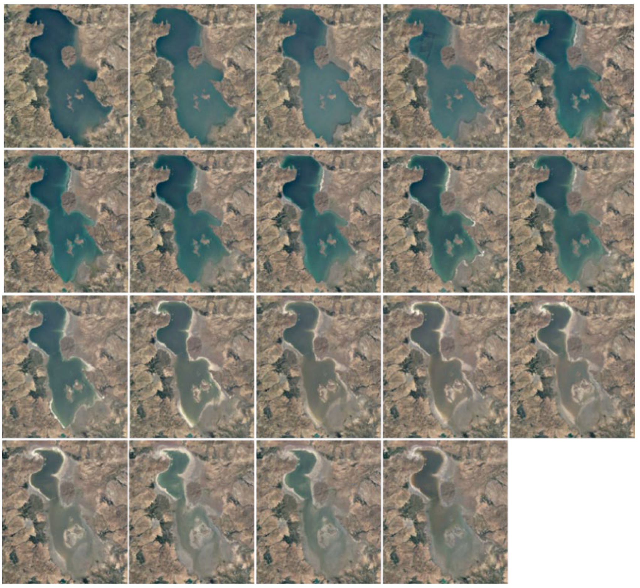
Land 12 01602 g001
Figure 2. Remote sensing panoramic historical images of Lake Urmia from 1996 to 2014 (image from Google Earth Pro Software).
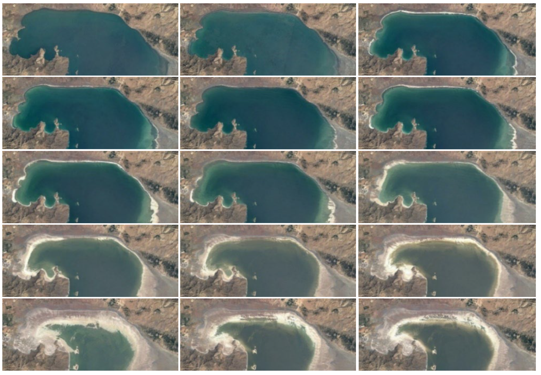
Land 12 01602 g002
Figure 3. Remote sensing partial historical images of Lake Urmia from 2000 to 2014 (image from Google Earth Pro Software).
Land 12 01602 g003
Figure 4. Results of image segmentation and image binarization of remote sensing images of Lake Urmia in 2000.
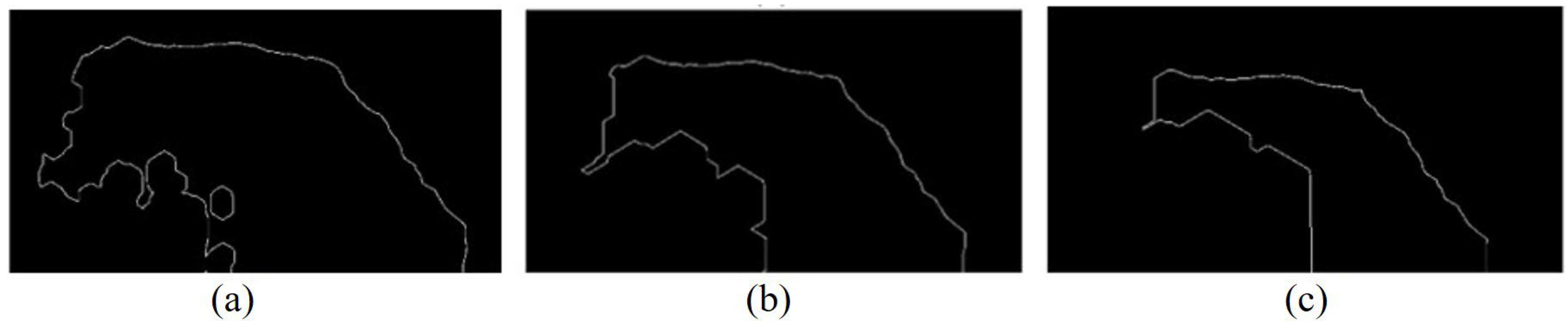
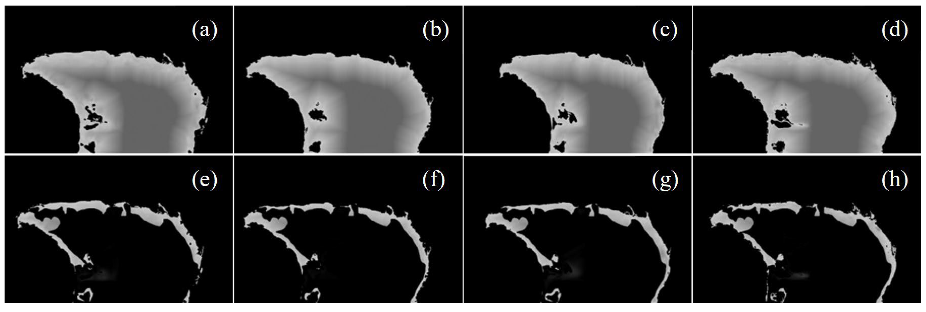
Land 12 01602 g004
Figure 5. Partial results of the 2000 binarization image of Lake Urmia after erosion. (a) The result of the 10th erosion; (b) the result of the 30th erosion; (c) the result of the 50th erosion.
Land 12 01602 g005
Figure 6. Partial difference image after erosion of binarization image of Lake Urmia in 2000. (a) The image of the difference between the 9th erosion and the 10th erosion results; (b) the image of the difference between the 29th and 30th erosion results; (c) the image of the difference between the 49th and 50th erosion results.
Land 12 01602 g006
Figure 7. U-Net-STN model prediction process.
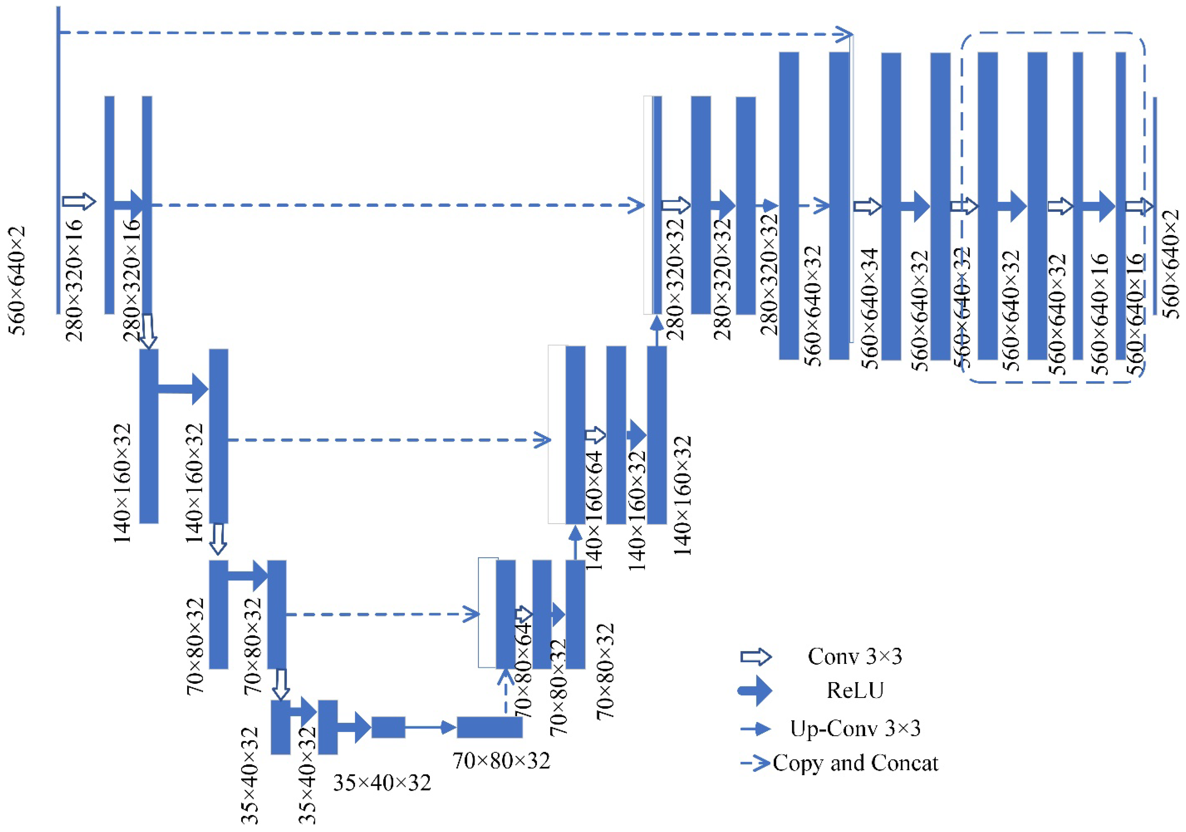
Land 12 01602 g007
Figure 8. U-Net structure diagram.
Land 12 01602 g008
Figure 9. Network structure diagram of the evolutionary feature extraction module.
Land 12 01602 g009
Figure 10. Schematic diagram of prediction flow of spatial transformation module.
Land 12 01602 g010
Figure 11. Schematic diagram of DICE indicator calculation.
Land 12 01602 g011
Figure 12. Comparison results of regularization parameter α of evolution field: (a,b) are the true images of 2013 and 2014, respectively; (c,d) is the prediction of 2014 when α is 0.01 and 0.1, respectively.
Land 12 01602 g012
Figure 13. Comparison of prediction result of Experiment 1. (a) Difference image between (b,c); (b) prediction results using data from the first 2 years; (c) ground truth image for the year 2001; (d) prediction results using data from the first 5 years; (e) difference image between (d,c); (f) difference image between (g,h); (g) prediction results using data from the first 2 years; (h) ground truth image for the year 2006; (i) prediction results using data from the first 12 years; (j) difference image between (i,h); (k) difference image between (l,m); (l) prediction results using data from the first 2 years; (m) ground truth image for the year 2011; (n) prediction results using data from the first 15 years; (o) difference image between (n,m).
Land 12 01602 g013
Figure 14. Experiment 2 predictive results comparative diagram. (a) Difference image for (b,c); (b) predicted results using data from the first 2 years; (c) ground truth image for the year 2010; (d) predicted results using data from the first 5 years; (e) difference image between (d,c); (f) difference image between (g,h); (g) predicted results using data from the first 2 years; (h) ground truth image for the year 2011; (i) predicted results using data from the first 6 years; (j) difference image between (i,h); (k) difference image between (l,m); (l) predicted results using data from the first 2 years; (m) ground truth image for the year 2012; (n) predicted results using data from the first 7 years; (o) difference image between (n,m).
Land 12 01602 g014
Figure 15. The time series image prediction results. (a) Prediction of 2014 using previous 4 years’ data; (b) prediction of 2014 using previous 7 years’ data; (c) prediction of 2014 using previous 10 years’ data; (d) prediction of 2014 using previous 14 years’ data; (e) prediction of 2014 using previous 18 years’ data; (f) the difference image between (a) and true 2014 image; (g) the difference image between (b) and true 2014 image; (h) the difference image between (c) and true 2014 image; (i) the difference image between (d) and true 2014 image; (j) the difference image between (e) and true 2014 image.
Land 12 01602 g015
Figure 16. The relationship between ACC, DICE, MSE, and time step n.
Land 12 01602 g016
Figure 17. The time series prediction results. (a) Prediction of 2014 using previous 5 years’ data; (b) prediction of 2014 using previous 6 years’ data; (c) prediction of 2014 using previous 7 years’ data; (d) prediction of 2014 using previous 8 years’ data; (e) the difference image between (a) and true 2014 image; (f) the difference image between (b) and true 2014 image; (g) the difference image between (c) and true 2014 image; (h) the difference image between (d) and true 2014 image.
Land 12 01602 g017
Figure 18. Comparison of experimental results using pre-processed images and original images: (a) pre-processed ground truth image for the year 2014; (b) predicted results using pre-processed images from 5 years; (c) difference image between (a,b); (d) predicted results using pre-processed images from 9 years; (e) difference image between (a,d); (f) predicted results using pre-processed images from 13 years; (g) difference image between (a,f); (h) original ground truth image for the year 2014; (i) predicted results using original images from 5 years; (j) difference image between (h,i); (k) predicted results using original images from 9 years; (l) difference image between (h,k); (m) predicted results using original images from 13 years; (n) difference image between (h,m).
Land 12 01602 g018
Figure 19. Comparison of the results of the prediction experiment using the pre-processed image and the original image for training, and the original image. (a) The result of using the original image training and original image prediction; (b) the real image; (c) the simulation result of using the pre-processed image training and original image prediction.
Land 12 01602 g019
Table 1. Prediction and evaluation indexes of time series images in C o l 1 .
Predict 2001ACCMSEDICE
2 years image0.8132440.950.9786
5 years image0.8147451.900.9787
Predict 2006ACCMSEDICE
2 years image0.8462585.260.9643
10 years image0.8486453.930.9714
Predict 2011ACCMSEDICE
2 years image0.8770507.350.9603
15 years image0.8772451.560.9622
Table 2. Prediction and evaluation indexes of time series images in C o l 2 .
Predict 2010ACCMAEDICE
2 years image0.7410.650.9592
5 years image0.758.810.9758
Forecast 2011ACCMAEDICE
2 years image0.7514.010.9550
6 years image0.7612.620.9682
Predict 2012ACCMAEDICE
2 years image0.8010.470.9447
7 years image0.824.870.9673
Table 3. Prediction and evaluation indexes of time series images in the first 4, 7, 10, 14, and 18 years of model use.
Predict 2014ACCMSEDICE
4 years image0.8888376.590.9595
7 years image0.8916363.570.9602
10 years image0.8901409.290.9603
14 years image0.8915398.750.9616
18 years image0.8943234.790.9636
Table 4. Prediction and evaluation indexes of 5, 6, 7, and 8 year time series images used in the model.
Predict 2014ACCMSEDICE
5 years image0.79141751.810.9329
6 years image0.79301643.690.9347
7 years image0.79501686.090.9361
8 years image0.79831526.300.9407
Table 5. Prediction and evaluation indexes of the original image and pre-processed image used in the model.
Predict 2014ACCMSEDICE
5 years of pre-processed images0.8896406.490.9605
5 years original image0.402491.160.8894
9 years of pre-processing images0.8896391.180.9673
9 years original image0.372571.770.8955
13 years of pre-processing images0.8934226.570.9714
13 years original image0.367777.540.8827
Table 6. The model uses the original image and pre-processed image training prediction evaluation index.
Predict 2014ACCMSEDICE
18 years of pre-processed images0.614467.530.8950
18 years original image0.4658139.600.8765
Disclaimer/Publisher’s Note: The statements, opinions and data contained in all publications are solely those of the individual author(s) and contributor(s) and not of MDPI and/or the editor(s). MDPI and/or the editor(s) disclaim responsibility for any injury to people or property resulting from any ideas, methods, instructions or products referred to in the content.

