Article

The Effect of Ornamental Groundcover Habit and Irrigation Delivery on Dynamic Soil Conditions

Louisiana State University Agricultural Center, Hammond Research Station, Hammond, LA 70403, USA
*
Author to whom correspondence should be addressed.
Land 2023, 12(6), 1119; https://doi.org/10.3390/land12061119
Submission received: 21 April 2023 / Revised: 15 May 2023 / Accepted: 19 May 2023 / Published: 24 May 2023
(This article belongs to the Section Landscape Ecology)

Abstract

:
Sustainable landscapes provide environmental, social, and financial benefits, with interest and adoption increasing due to environmental awareness. Ornamental ground-cover systems have garnered interest in the landscape due to the reduced need for water, fertilizers, pesticides, and maintenance compared to typical landscapes; however, limited research on groundcover ability to modulate soil conditions or suppress weeds exists. This study explored how ornamental groundcover systems impact the sustainability of landscapes. The effects of ground-cover growth habit (matting; bunching) and irrigation delivery method (micro spray; overhead) on soil temperature, volumetric water content (VWC), and electric conductivity (EC), along with impacts on weed growth, soil microbial communities, and plant coverage, were measured. Soil temperatures were generally lower under groundcover species with a matting growth habit, and to a lesser extent, bunching growth habits, in comparison to the warmer fallow systems. Groundcovers with a matting form led to lower VWC values compared to taxa with other growth habits, particularly when micro-irrigated. Plant form did not significantly influence EC values; however, micro spray irrigated plots had significantly higher EC values, likely attributed to irrigation spray patterns. Micro spray irrigation in tandem with matting growth habit taxa decreased weed density more effectively than taxa with bunching growth habits or groundcovers maintained under overhead irrigation. Selection of groundcover species with greater foliar coverage along with implementing more efficient irrigation practices can decrease soil temperatures, soil moisture, and weed density. Incorporating groundcovers in the landscape can decrease maintenance requirements and water/chemical use, thus increasing sustainability and decreasing environmental consequences.

1. Introduction

Sustainable practices such as reducing the use of, and reliance on, critical inputs such as water, energy, and chemicals are gaining widespread adoption in the landscape industry as consumers request sustainable practices to be incorporated into their landscapes. Sustainable practices often manifest as reduced water, fertilizer, pesticides, and maintenance. Sustainable landscapes are increasingly being adopted and recognized for their potential to enhance ecological, social, and educational benefits in urban and suburban landscapes [1]. Across the globe, urban areas are exponentially increasing with much of this growth occurring in developing countries, which are predicted to harbor 80% of the global urban population by 2030 [2]. Urban areas are similarly expanding within the United States, increasing the need to implement sustainable practices within our landscapes. Encouraging the installation of landscapes that require fewer inputs (e.g., irrigation, fertilizer, and pesticides) may decrease negative environmental outcomes. This is particularly relevant to cities, where limited water supplies are generating more interest in identifying plants for the landscape that do not require as much water as some industry standard taxa [3]. Mismanaging fertilizer in urban landscapes represents a potential source of nutrients that may contribute to water quality impairment [4]. Fertilizing lawns can contribute to non-point source pollution, degrading water resources via eutrophication [5].
With landscapes currently occupying millions of acres of land in the United States, it is imperative that we continue to develop and implement new sustainable landscape practices to maximize the ecological value of this land. The pre-eminent component in the American landscape is the lawn, a notoriously high input feature, covering an estimated 1.9% of the U.S. [6]. The lawn is ubiquitous throughout the American landscape [7], comprising 10 to 16 million hectares of land in the U.S. [8]. Lawns have historically been associated with high rates of water, fertilizer, and maintenance [9]. Reducing lawn areas, either through conversion to native planting schemes or replacing turfgrass species with turfgrass alternatives, can improve landscape sustainability. These non-turf grass species are popularly known as ornamental groundcovers. Planting and maintaining ornamental groundcovers may reduce water use [10], pesticide use [11], and labor [12] compared to turfgrass, and provide the added benefit of use as forage for pollinators [13].
An ornamental groundcover is defined as an intentionally cultivated plant species that has a dense, prostrate growth habit, often with adventitious roots, and which can survive where turfgrass cannot. Incorporating ornamental groundcover systems into landscapes can reduce labor costs, maintenance, water and fertilizer usage, and on-site runoff water [14,15]. Many ornamental groundcovers are perennial species that can survive for several growing seasons and do not require annual planting, therefore reducing labor costs [12]. Ornamental groundcovers are a weed control alternative to mulches and provide several distinct advantages. All mulches, organic or synthetic, must be maintained periodically, adding to labor and maintenance requirements. Although many organic materials can exclude light if applied at sufficient depth, they degrade over time and certain materials may potentially attract pests [16].
Public and private gardens are a major component of urban green space and can provide considerable improvements to ecosystem biodiversity [2]. Landscapes have often been slower to adopt sustainable practices than production agriculture [17]. However, with increased urbanization, ornamental plantings in these areas are expected to increase as cities continue to beautify public and private places. As land is converted from areas traditionally covered by vegetation into a built environment, groundcovers could be an essential tool in maintaining the vegetative cover of the land. Impervious surfaces accompany urban development [18], most commonly in the form of roofs, parking lots, and roads [19]. These impervious surfaces have dramatic effects on water movement, such as stormwater flow [20]. By substituting impervious surfaces with permeable surfaces such as groundcover plantings, water infiltration and stormwater mitigation could be improved.
Cover crops have similar environmental functions to ornamental groundcovers and are often utilized to manage soil erosion, runoff, soil nutrients, soil physical properties, soil water, soil organic carbon, soil chemical properties, and soil biology in agricultural settings [21,22,23]. Incorporating cover crops into fields can remove water and nitrogen from the soil profile through transpiration and nitrogen uptake [24]. Excess water in the soil profile is not conducive to plant growth because of reduced soil oxygen levels which impede root growth [25]. Cover crops are also used to reduce weed pressure in many cropping systems by changing residue amounts and adding competition for water, nutrients, and sunlight [26]. It is understood that similarities between cover crops and ornamental groundcovers exist; however, there are several unique differences between these two systems.
Groundcover management systems have been used to improve agronomic crop fields, tree fruit orchards, and other production agriculture; however, they have not been studied to the same extent in the landscape. Therefore, the objective of this experiment was to study the influence of ornamental groundcovers on soil health and conditions, and to quantify various environmental, cultural, or economic benefits that may be associated with groundcover plantings. Additionally, this research aims to understand how groundcover growth habits and irrigation application methods influence the landscape.

2. Materials and Methods

2.1. Site Preparation and Establishment

An 80 m2 area plot (4 m × 20 m) was prepared at the Louisiana State University Agricultural Center Hammond Research Station located in Hammond, LA, USA (30.5044° N, 90.4612° W). Wherein, the soil, a fine-loamy, siliceous, semiactive, thermic typic Hapludult, was intensively cultivated to a depth of 10 cm and amended with a locally sourced landscape mix consisting of pine bark, sand, dolomitic lime, micro-nutrient blend, and magnesium sulfate to provide uniform conditions for plant establishment (Phillips Bark Processing Company; Brookhaven, MS, USA). Eighteen individual one m2 plots were partitioned, with 50 cm between plots north to south and one meter separating the two rows of plots east to west, and also three meters were placed between irrigation treatment. The plots were subdivided into two separate irrigation regimes, where half the plot was designed for overhead irrigation and the other half plot was designed for micro-irrigation.

2.2. Irrigation

The overhead irrigation consisted of sprayers (Model 15 UH; U15Q, Rainbird, Azusa, CA, USA) on six, 1.0 m risers with four corner risers and two middle risers located 4.5 m toward the center of the overhead plot. The micro-irrigation plots were designed with a 360-degree sprayer (Model XS360TS Adj True Spray, Rainbird, Azusa, CA, USA) on a 30 cm Riser with barb 0.16 adapter (Antelco, Longwood, FL, USA) positioned in the center of each plot. Distribution uniformity (DU) tests were conducted in each zone following [27]. The overhead DU was 77%, and the micro-irrigation had a DU of 89.5%.
Irrigation was applied to each plot twice a week (Monday at 9 a.m. and Thursday at 9 a.m.), with plots in both irrigation delivery treatments receiving 6.8 L/m2 of water per irrigation event. To ensure equal irrigation applications, the overhead plots were irrigated for 15 min, and the micro-irrigation plots were irrigated for 22 min every event.

2.3. Plant Materials and Installation

A soil moisture sensor (Teros 12; METERGROUP, Pullman, WA, USA) was installed in the center of each plot at a depth of 15 cm beneath the soil surface to monitor soil volumetric water content, temperature, and electric conductivity (EC) in undisturbed soil. The sensors were attached to a data logger (CR1000x; Campbell Scientific, Logan, UT, USA) along with a tipping bucket rain gauge (TR-525I; Texas Electronics, Dallas, TX, USA), which collected data every 10 min. The data logger was programmed to record the hourly averages of each sensor. The entire research plot was mulched with pine straw at a depth of 7.5 cm. Within each irrigation system, three randomly selected plots were assigned plantings with Sphagneticola trilobata (Wedelia), three were planted with Liriope muscari ‘Big Blue’ (Liriope), and the remaining three were left fallow, resulting in three replicate plots of each treatment combination (n = 3 for Fallow: Overhead, Fallow: Microirrigation, Liriope: Overhead, Liriope: Microirrigation, Wedelia: Overhead, and Wedelia: Microirrigation, respectively).
The Wedelia was selected as a quick-growing groundcover with a matting habit, which would spread across the surface of the plot representing an established groundcover planting and potentially intercepting water. Liriope was selected as a bunching groundcover, with a form that could direct water into the soil. Each plot had nine individual plants, spaced on 30 cm centers using a cardboard bracket as a template. After planting, each plot received 100 g of controlled release fertilizer (Osmocote Plus 15-9-12, 5–6 months; ICL Specialty Fertilizers, Dublin, OH, USA), which was spread uniformly across the entire plot.

2.4. Coverage Analysis

Overhead photographs of each plot were collected every 30 d ± 3 d utilizing a digital camera (A6000; Sony Group Corporation, Tokyo, Japan). A 1 m × 1 m bracket with a stand was constructed to ensure the camera was positioned 150 cm high above the center of the plots to ensure each photograph was taken from the same height with the entire one m2 plot within the frame. This bracket also served as a border for further analysis. A portable canopy was placed over plots to ensure that sunlight levels were consistent for every photo. Individual photographs were cropped using Adobe Photoshop (Adobe Inc., San Jose, CA, USA) to only include the materials within the bracket. Photos were analyzed using WinCAM Color Area Meter Software Pro 2020a 32-bit (Regent Instruments, Québec City, QC, Canada), wherein the plot coverage of the plants was calculated. Color classes were assigned to the groundcover and the background, with software analysis used to determine percentage.

2.5. Weed Density and Biomass

Weed suppression was assessed through collecting individual weeds every two weeks starting on 25 May 2022 and concluding on 14 September 2022. A bracket was placed around each plot. Weeds were only collected within the 1 m2 plot. Weeds were severed at the soil level to minimize soil disturbance. Weeds were counted and organized as either a monocotyledon or dicotyledonous species. Weeds were dried at 70 °C for 7 d and the dry weight was recorded. This was a modified protocol based on work performed by Cardina et al. [28]. Glyphosate herbicide was applied to the lawn edge of the study area every three weeks to prevent weed encroachment, but no herbicides were applied within plots.

2.6. Microbial Communities

Analysis of the soil microbial communities in this project was completed using the Fatty Acid Methyl-Ester (FAMEs) technique described by [29]. Soil cores 30 cm in length were extracted from each plot 30 cm from the center of each plot in the southwest corner on 17 June 2022 (Week 6) and again on 23 September 2022 (Week 19). The samples were frozen immediately after removal from the soil. On the day of the extraction, each sample was mixed in each collection bag to homogenize the mixture. The fatty acid methyl-esters were extracted from each 3 g sample. These were then processed through a gas chromatograph (7890B, Agilent), which measured the relative and absolute abundance of each class of soil microorganisms. The peaks were measured using Sherlock™ Microbial Identification System software (MIDI, Microbial ID, Inc., Newark, DE, USA).

2.7. Data Analysis

The data presented in tables and figures with associated statistics were analyzed in JMP Pro (16.1.0; SAS Institute, Inc.; Cary, NC, USA) utilizing Tukey’s Honestly Significant Difference (α = 0.05) to separate plant coverage means, VWC means, temperature means, EC means, soil microbial community abundance means, and weed density and biomass means across three plot treatment responses across both irrigation deliveries. Analysis of variance was further utilized to determine any statistically significant differences between the means of the three plots.

3. Results and Discussion

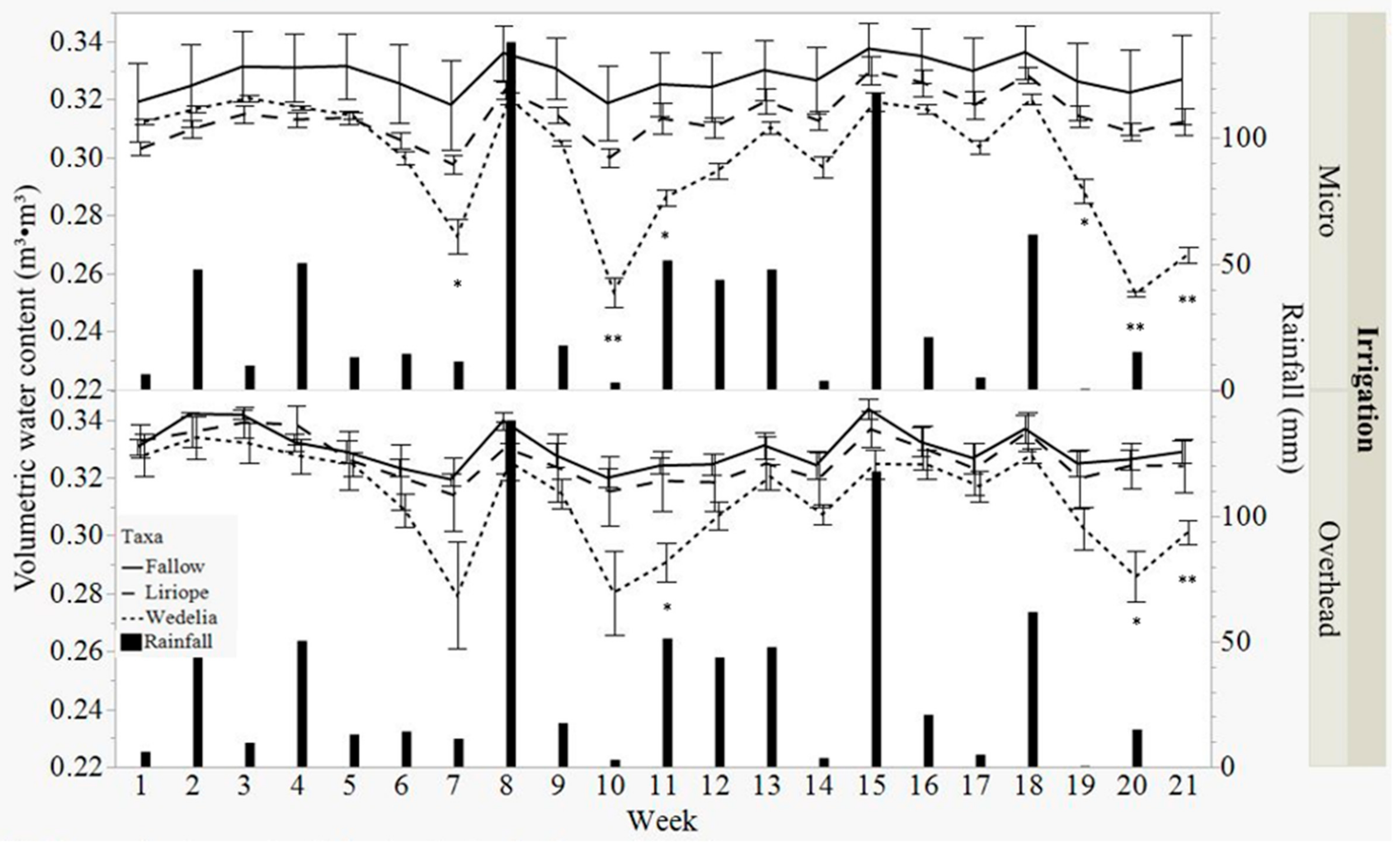
3.1. Volumetric Water Content

Water movement under different groundcover management systems (GMSs) has been well-studied. Several comprehensive reviews assessing the relative advantages and disadvantages of various GMSs have emphasized the need for additional information on the physiological, economic, and edaphic impacts of GMSs [30]. Throughout the study, Wedelia plots were observed to have a lower VWC value compared to Liriope, including being significantly lower on 6 of 21 measurement days under micro-irrigation. This trend was also observed in overhead irrigation, but to a less pronounced extent (Figure 1).
Ornamental groundcovers function similarly to cover crops, where more total plant biomass produces a higher transpiration rate resulting in less water in the soil profile. Kahimba et al. [31] demonstrated that cover crops can reduce excess soil moisture Moreover, Yunusa et al. [32] demonstrated that greater root biomass and leaf area index (LAI) results in increased transpiration rates. Groundcover biomass was not measured during this study; however, an alternative metric, vegetative cover, measured that Wedelia plots had a range of 9–52% more vegetative coverage than Liriope plots (Table 1), yielding lower minimum VWC values for plots with Wedelia (Figure 2).
VWC was greatest under the fallow plots (Figure 3), as there were no plant roots to remove water [33] from the soil profile. Considerable variation in VWC was observed under the fallow plots, likely attributed to the lack of vegetation increasing water infiltration into soil [34]. Liriope is a plant species that has a relatively low water demand, thus reducing water uptake and maintaining higher soil VWC values than plots with Wedelia [35]. The average maximum VWC of the soil was lower in plots receiving micro spray irrigation compared to plots receiving overhead irrigation, despite identical volumes of water being applied. Similar results were observed by Rowe et al. [36], where areas receiving overhead irrigation had greater VWC values when compared to other irrigation methods. Over the first five weeks of the study, plots receiving micro spray irrigation exhibited increases in the maximum VWC values while the overhead irrigated plots remained stable (Figure 3). During weeks 6 and 7, VWC in all plots decreased due to an irrigation malfunction resulting in no irrigation applied for an estimated 2 weeks.
Flux (VWCMax-VWCMin) average values were observed to be greatest in both irrigation deliveries for Wedelia plots, noting a greater change in VWC for Wedelia versus both Liriope and fallow plots following rainfall events (Figure 4). Moreover, during periods of rainfall greater than or equal to 50 mm during the week, VWC values increased for all treatments, but most dramatically for plots with Wedelia receiving micro irrigation, and to a slightly lesser extent plots with Wedelia receiving overhead irrigation, which was likely attributed to root turnover creating macropores thus increasing the infiltration rate [37,38,39]). Interspace areas between micro spray irrigation plots may have been drier than over-head irrigated areas due to the higher water application efficiency of micro spray irrigation [40], unlike overhead irrigation where water was applied intentionally to the plots and unintentionally to the plot interspaces. The low moisture interspaces, along with the drier soil created by the high-water demand of the plots planted with Wedelia, may have increased the infiltration rate due to the soil’s initial lower soil moisture values [41,42].

3.2. Soil Temperature

Groundcovers have been shown to reduce high soil temperatures, which factor into the rates of biochemical reactions and have strong influences on plant and root growth [43]. The plots with Wedelia had the lowest temperatures under both irrigation delivery systems, followed by plots planted with Liriope, and finally plots left fallow (Figure 5). Wedelia had a greater coverage percentage (Table 1) which likely contributed to more reflected solar radiation from the soil surface, which would be similar to results observed by Van Huyssteen et al. [44]. The increased shading caused by the greater plot coverage provided by the dense Wedelia canopy likely contributed to the lower temperatures in soils under both irrigation systems [45]. A higher evaporative demand from the plants may have also lowered the soil temperature under plots planted with Wedelia [46]. This is mirrored by the lower soil moisture content within the Wedelia plots (Figure 2). The fallow plots generally had higher temperatures when compared to plots planted with Liriope or Wedelia under both irrigation deliveries, which was consistent with results from similar studies [47,48]. During weeks of rainfall greater than or equal to 50 mm, ambient air temperatures were lower or equal to soil temperatures in all treatments. This increased water content within the treatments may have raised the specific heat of the soil [49]. As average ambient temperatures decreased below 26 °C during the fall, soil temperatures under all treatments were greater than air temperature, which is consistent with observations from a study by Yang et al. [50].

3.3. Electric Conductivity

Electrical conductivity (EC) is the measure of soluble salts in a soil [51]. Measuring EC is a fast and cost-effective method to determine several chemical properties of soil including leaching and irrigation patterns and it can correlate to crop yields [52]. There were no significant differences between the planting treatments receiving micro spray or overhead irrigation (Figure 6). Micro irrigated plots had significantly lower EC values (p < 0.0001) than plots receiving overhead irrigation, indicating that overhead irrigation more than likely leached more nutrients than micro spray irrigation due to irrigation efficiency and distribution [53,54]. Variability in the composition of the soil [55] could have led to an increased EC value under micro spray irrigation but was not measured because of the small zone of influence of the soil sensors (1010 mL). Plots planted with Liriope had significantly higher EC values (p < 0.0001) in comparison to Wedelia plots or fallow plots presumably due to the roots of Liriope increasing the EC values [56].

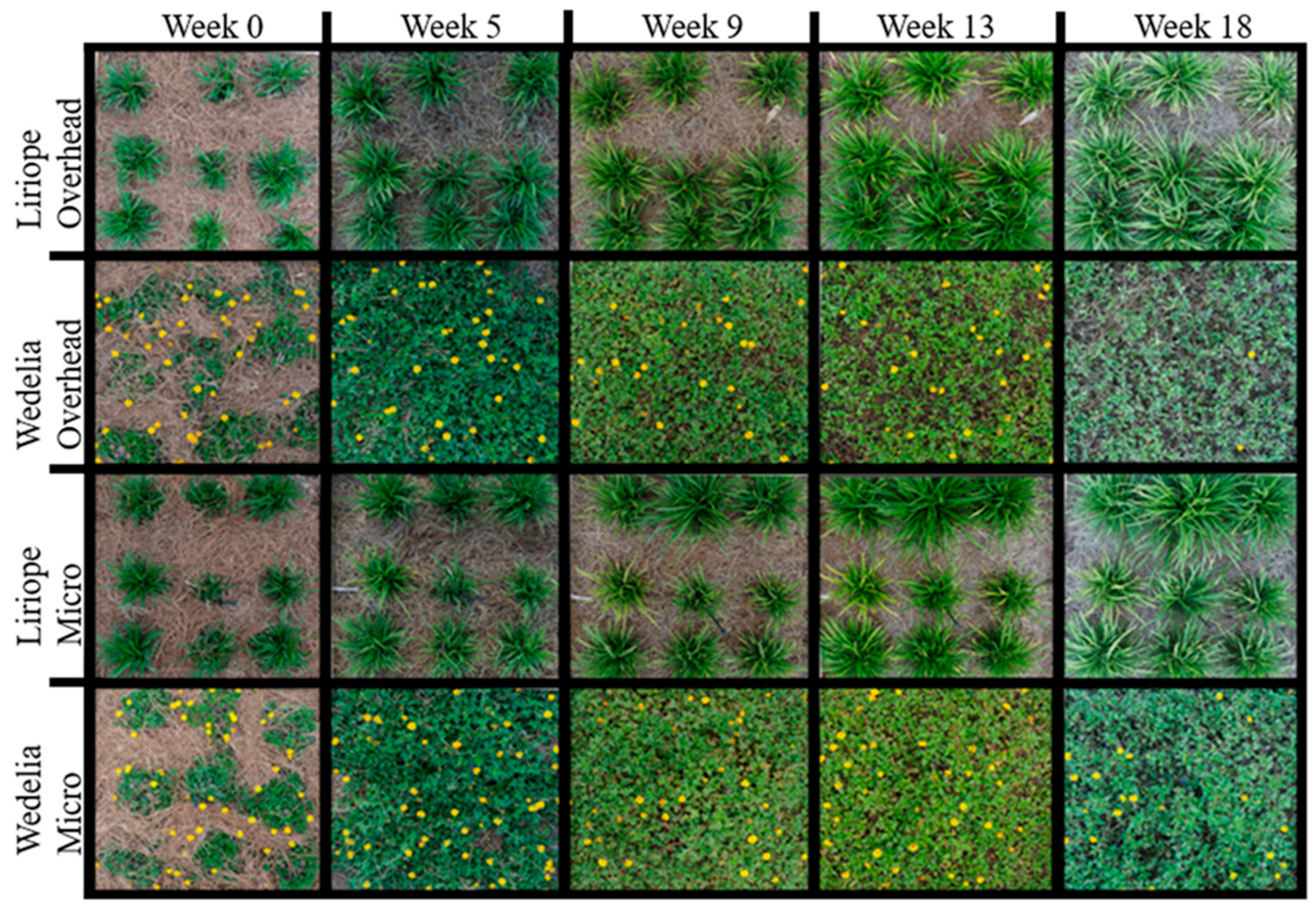
3.4. Vegetative Coverage

Wedelia had significantly more coverage than Liriope on three of the five dates this metric was measured during the study (Table 1). Wedelia has a more rapid growth rate and spreading growth form than Liriope, contributing to the observed greater coverage [57,58]. Irrigation delivery method did not influence the coverage percentage of the two species. Differences in the growth habits of Wedelia and Liriope were most likely attributable to the innate form of each species, and less so towards the irrigation application method.

3.5. Weed Biomass and Density

Fallow plots irrigated via overhead systems exhibited increased levels of weed density and weed biomass when compared to plots planted with Wedelia or Liriope (Table 2), which is consistent with results demonstrated in other agricultural systems [59,60]. The Wedelia and Liriope planted plots provided coverage with their respective canopies, with Wedelia providing more coverage than the plots planted with Liriope. Wedelia has a horizontal growth pattern with less erect growth than Liriope (Figure 7), decreasing light transmittance to the soil and likely contributing to decreased weed biomass and density [61,62]. The combination of, and interaction between, the increased shading and lower moisture content (Figure 2) created by the Wedelia plants produced an environment that was less conducive to weed germination and growth [63,64,65].
Micro-irrigated plots that were planted with Wedelia or Liriope, or micro-irrigated plots left fallow, had less weed density and biomass than overhead irrigated plots; however, the fallow plots did not have consistently higher levels of weed density and biomass as is demonstrated in the overhead irrigation. Considering both irrigation systems delivered the same volume of irrigation water, and that coverage percentages did not differ between irrigation delivery systems (Table 1), it is possible that irrigation distribution influenced differences in weed density and biomass [66,67]. The more precise irrigation only irrigated the planted areas and intentionally prevented irrigating the non-intentional areas where weeds could germinate.

3.6. Microbial Communities

Plant cover or cover crops can have a sizeable impact on soil microbial populations. The rhizosphere is the area immediately surrounding plant roots and their associated microbial community [68]. The rhizosphere is often rich with microbial life due to root photosynthate secretions [69,70,71]. Consistent with findings by Buyer et al. [72], no significant differences were observed in relative or absolute abundance among the microbial communities between plant species when soils were sampled during week 6 or week 20 (Table 3). Buyer et al. [72] observed that the rhizosphere of plants only affects a small fraction of the microbial community, and any changes in root biomass and species would be insufficient to significantly alter the community. Additionally, no significant differences were observed in relative or absolute abundance among the microbial communities between irrigation methods. Soil moisture has been found to influence microbial communities [73]; however, applied irrigation did not differ between delivery systems nor was rainfall deficit enough to influence the communities. Ignoring all treatment variables (plot, irrigation method, interaction), Gram-negative bacteria and arbuscular mycorrhizae were more relatively abundant when soil was sampled during week 20; however, eukaryotes were more abundant during week 6. It is hypothesized that the plots were too close in proximity to achieve differences, considering spatial variability can directly influence microbial community structures and similar communities dissipate with increasing distance [74]. The entire study site was 80 m2 with 50 cm between plots within irrigation treatments with 20 m being the furthest distance between two plots and distances of at least 25 m apart were observed to detect any differences in soil microbes [75]. Plant roots, moisture levels, and distance between locations can indeed influence soil microbial communities, yet within the scope of this study these factors did not vary sufficiently to alter community structures.

4. Conclusions

Groundcover plant species are a low-maintenance alternative to the turfgrass that typically dominates large areas of the landscape. Turfgrass requires substantial labor, water, and chemical inputs to maintain an aesthetic appeal; however, substituting turf with groundcovers provides the opportunity to reduce the demand of these costly resources. The investigated groundcovers demonstrated success in modulating soil conditions, particularly in buffering soil temperatures between seasons and maintaining optimal soil moisture levels. This research also highlights how fast-growing ornamental species with a matting growth habit are particularly effective at reducing weed pressures in the landscape, especially when used in conjunction with precision irrigation. Groundcovers provide a unique opportunity to replace turf areas that are hard to access, costly to maintain, or suffer from excessive or substandard drainage. Further research quantifying the benefits of groundcovers, including studying other ornamental groundcover species and their suitability for erosion control, pollution abatement, and pollinator forage, as well as multi-year, longitudinal studies are necessary for advancing their use. Through purposeful selection of site-specific groundcover species and installation of efficient irrigation delivery systems, a less intensive, more sustainable landscape can be cultivated.

Author Contributions

Conceptualization, J.S.F.; methodology, J.S.F., T.M.M. and D.E.A.; software, T.M.M.; validation, T.M.M., D.E.A. and J.S.F.; formal analysis, T.M.M.; investigation, T.M.M.; editing, J.S.F. and D.E.A.; visualization, T.M.M. and D.E.A.; supervision, J.S.F.; project administration, J.S.F.; funding acquisition, J.S.F. All authors have read and agreed to the published version of the manuscript.

Funding

This research was funded in part by the Louisiana Nursery and Landscape Foundation for Scholarship and Research and the Louisiana Agricultural Experiment Station.

Data Availability Statement

Data will be made available upon request.

Acknowledgments

The authors would like to thank the faculty and staff of the Hammond Research Station who assisted with the administration of this project and supported data collection. We would like to thank Jeff Kuehny and Heather Kirk Ballard for their support of T.M. McKeown’s graduate program and Lisa Fultz for assistance with soil microbiology analysis.

Conflicts of Interest

The authors declare no conflict of interest. The funders had no role in the design of this study, in the collection, analyses, or interpretation of data, in the writing of the manuscript, or in the decision to publish the results.

References

  1. Saksa, K.A.; Ilvento, T.W.; Barton, S.S. Interpretation of Sustainable Landscapes Affects Student Perception of Sustainable Landscape Features. Horttechnology 2012, 22, 402–409. [Google Scholar] [CrossRef]
  2. Goddard, M.A.; Dougill, A.J.; Benton, T.G. Scaling up from gardens: Biodiversity conservation in urban environments. Trends Ecol. Evol. 2010, 25, 90–98. [Google Scholar] [CrossRef] [PubMed]
  3. Staats, D.; Klett, J.E. Water Conservation Potential and Quality of Non-turf Groundcovers versus Kentucky Bluegrass under Increasing Levels of Drought Stress. J. Environ. Hortic. 1995, 13, 181–185. [Google Scholar] [CrossRef]
  4. Carey, R.O.; Hochmuth, G.J.; Martinez, C.J.; Boyer, T.; Nair, V.D.; Dukes, M.; Toor, G.S.; Shober, A.; Cisar, J.L.; Trenholm, L.E.; et al. A Review of Turfgrass Fertilizer Management Practices: Implications for Urban Water Quality. Horttechnology 2012, 22, 280–291. [Google Scholar] [CrossRef]
  5. Campbell, J.; Rihn, A.; Khachatryan, H. Factors Influencing Home Lawn Fertilizer Choice in the United States. Horttechnology 2020, 30, 296–305. [Google Scholar] [CrossRef]
  6. Milesi, C.; Running, S.W.; Elvidge, C.D.; Dietz, J.B.; Tuttle, B.T.; Nemani, R.R. Mapping and Modeling the Biogeochemical Cycling of Turf Grasses in the United States. Environ. Manag. 2005, 36, 426–438. [Google Scholar] [CrossRef]
  7. Larson, K.L.; Brumand, J. Paradoxes in landscape management and water conservation: Examining neighborhood norms and institutional forces. Cities Environ. 2014, 7, 6. Available online: https://digitalcom-mons.lmu.edu/cate/vol7/iss1/6 (accessed on 2 October 2022).
  8. Steinberg, T. Lawn and Landscape in World Context, 1945–2000. OAH Mag. Hist. 2005, 19, 62–69. [Google Scholar] [CrossRef]
  9. Yue, C.; Cui, M.; Watkins, E.; Patton, A. Investigating Factors Influencing Consumer Adoption of Low-input Turfgrasses. Hortscience 2021, 56, 1213–1220. [Google Scholar] [CrossRef]
  10. Burayu, W.; Umeda, K. Versatile Native Grasses and a Turf-Alternative Groundcover for the Arid Southwest United States. J. Environ. Hortic. 2021, 39, 160–167. [Google Scholar] [CrossRef]
  11. Garber, M.; Bondari, K. Landscape Maintenance Firms: II. Pest Management Practices. J. Environ. Hortic. 1996, 14, 58–61. [Google Scholar] [CrossRef]
  12. Roka, F.M.; Rouse, R.E.; Miavitz-Brown, E. Economic considerations from using perennial peanut in urban landscapes. Proc. Fla. State Hortic. Soc. 2003, 116, 339–341. [Google Scholar]
  13. Masierowska, M.; Stawiarz, E.; Rozwałka, R. Perennial ground cover plants as floral resources for urban pollinators: A case of Geranium species. Urban For. Urban Green. 2018, 32, 185–194. [Google Scholar] [CrossRef]
  14. Marble, S.C.; Koeser, A.K.; Hasing, G. A Review of Weed Control Practices in Landscape Planting Beds: Part II—Chemical Weed Control Methods. Hortscience 2015, 50, 857–862. [Google Scholar] [CrossRef]
  15. Marble, S.C.; Pickens, J.M. Tolerance of Three Deep South Non-turf Ornamental Groundcovers to Applications of Postemergence Herbicides1. J. Environ. Hortic. 2020, 38, 91–100. [Google Scholar] [CrossRef]
  16. Marble, S.C.; Koeser, A.K.; Hasing, G.; McClean, D.; Chandler, A. Efficacy and Estimated Annual Cost of Common Weed Control Methods in Landscape Planting Beds. Horttechnology 2017, 27, 199–211. [Google Scholar] [CrossRef]
  17. Doxon, L.E. Landscape Sustainability: Environmental, Human, and Financial Factors. Horttechnology 1996, 6, 362–365. [Google Scholar] [CrossRef]
  18. Arnold, C.L., Jr.; Gibbons, C.J. Impervious Surface Coverage: The Emergence of a Key Environmental Indicator. J. Am. Plan. Assoc. 1996, 62, 243–258. [Google Scholar] [CrossRef]
  19. Shuster, W.D.; Bonta, J.; Thurston, H.; Warnemuende, E.; Smith, D.R. Impacts of impervious surface on watershed hydrology: A review. Urban Water J. 2005, 2, 263–275. [Google Scholar] [CrossRef]
  20. Brabec, E.; Schulte, S.; Richards, P.L. Impervious Surfaces and Water Quality: A Review of Current Literature and Its Implications for Watershed Planning. J. Plan. Lit. 2002, 16, 499–514. [Google Scholar] [CrossRef]
  21. Li, J.; Rao, M. Sprinkler water distributions as affected by winter wheat canopy. Irrig. Sci. 2000, 20, 29–35. [Google Scholar] [CrossRef]
  22. Kaspar, T.; Singer, J. The use of cover crops to manage soil. In Soil Management: Building a Stable Base for Agriculture; Hatfield, J.L., Sauer, T.J., Eds.; American Society of Agronomy and Soil Science Society of America: 5585 Guilford Road, Madison, WI, USA, 2011. [Google Scholar] [CrossRef]
  23. Rosario-Lebron, A.; Leslie, A.W.; Yurchak, V.L.; Chen, G.; Hooks, C.R. Can winter cover crop termination practices impact weed suppression, soil moisture, and yield in no-till soybean [Glycine max (L.) Merr.]? Crop Prot. 2019, 116, 132–141. [Google Scholar] [CrossRef]
  24. Strock, J.S.; Porter, P.M.; Russelle, M.P. Cover Cropping to Reduce Nitrate Loss through Subsurface Drainage in the Northern U.S. Corn Belt. J. Environ. Qual. 2004, 33, 1010–1016. [Google Scholar] [CrossRef] [PubMed]
  25. Pezeshki, S.R.; Delaune, R.D. Soil Oxidation-Reduction in Wetlands and Its Impact on Plant Functioning. Biology 2012, 1, 196–221. [Google Scholar] [CrossRef]
  26. Teasdale, J.R.; Brandsaeter, L.O.; Calegari, A.; Neto, F.S. Cover crops and weed management. In Non-Chemical Weed Management: Principles, Concepts and Technology; United States Department of Agriculture, Agricultural Research Service: Beltsville, MD, USA, 2007. [Google Scholar]
  27. Merriam, J.L.; Keller, J. Farm Irrigation System Evaluation: A Guide for Management; Utah State University: Logan, UT, USA, 1978. [Google Scholar]
  28. CardiNa, J.; Sparrow, D.H.; McCoy, E.L. Spatial Relationships Between Seedbank and Seedling Populations of Common Lambsquarters (Chenopodium album) and Annual Grasses. Weed Sci. 1996, 44, 298–308. [Google Scholar] [CrossRef]
  29. Quideau, S.A.; McIntosh, A.C.; Norris, C.E.; Lloret, E.; Swallow, M.J.; Hannam, K. Extraction and Analysis of Microbial Phospholipid Fatty Acids in Soils. J. Vis. Exp. 2016, 114, e54360. [Google Scholar] [CrossRef]
  30. Merwin, I.A.; Stiles, W.C.; Van Es, H.M. Orchard Groundcover Management Impacts on Soil Physical Properties. J. Am. Soc. Hortic. Sci. 1994, 119, 216–222. [Google Scholar] [CrossRef]
  31. Kahimba, F.C.; Ranjan, R.S.; Froese, J.; Entz, M.; Nason, R. Cover Crop Effects on Infiltration, Soil Temperature, and Soil Moisture Distribution in the Canadian Prairies. Appl. Eng. Agric. 2008, 24, 321–333. [Google Scholar] [CrossRef]
  32. Yunusa, I.A.M.; Zolfaghar, S.; Zeppel, M.J.B.; Li, Z.; Palmer, A.R.; Eamus, D. Fine Root Biomass and Its Relationship to Evapotranspiration in Woody and Grassy Vegetation Covers for Ecological Restoration of Waste Storage and Mining Landscapes. Ecosystems 2012, 15, 113–127. [Google Scholar] [CrossRef]
  33. Prasad, R. A linear root water uptake model. J. Hydrol. 1988, 99, 297–306. [Google Scholar] [CrossRef]
  34. Gerrits, A.M.J.; Pfister, L.; Savenije, H.H.G. Spatial and temporal variability of canopy and forest floor interception in a beech forest. Hydrol. Process. 2010, 24, 3011–3025. [Google Scholar] [CrossRef]
  35. Holmes, R. Taylor’s Master Guide to Gardening; Houghton Mifflin Harcourt: Boston, MA, USA, 2001. [Google Scholar]
  36. Rowe, D.B.; Kolp, M.R.; Greer, S.E.; Getter, K.L. Comparison of irrigation efficiency and plant health of overhead, drip, and sub-irrigation for extensive green roofs. Ecol. Eng. 2014, 64, 306–313. [Google Scholar] [CrossRef]
  37. Folorunso, O.; Rolston, D.E.; Prichard, T.; Louie, D.T. Cover crops lower soil surface strength, may improve soil permeability. Calif. Agric. 1992, 46, 26–27. [Google Scholar] [CrossRef]
  38. Krohn, N.; Ferree, D. Effects of Low-growing Perennial Ornamental Groundcovers on the Growth and Fruiting of ‘Seyval blanc’ Grapevines. Hortscience 2005, 40, 561–568. [Google Scholar] [CrossRef]
  39. Chalise, K.S.; Singh, S.; Wegner, B.R.; Kumar, S.; Pérez-Gutiérrez, J.D.; Osborne, S.L.; Nleya, T.; Guzman, J.; Rohila, J.S. Cover Crops and Returning Residue Impact on Soil Organic Carbon, Bulk Density, Penetration Resistance, Water Retention, Infiltration, and Soybean Yield. Agron. J. 2019, 111, 99–108. [Google Scholar] [CrossRef]
  40. Irmak, S.; Odhiambo, L.O.; Kranz, W.L.; Eisenhauer, D.E. Irrigation Efficiency and Uniformity, and Crop Water Use Efficiency. The Board of Regents of the University of Nebraska: Lincoln, NE, USA, 2011. Available online: https://digitalcommons.unl.edu/bio-sysengfacpub/451 (accessed on 25 October 2022).
  41. Horton, R.E. An Approach Toward a Physical Interpretation of Infiltration-Capacity. Soil Sci. Soc. Am. J. 1941, 5, 399–417. [Google Scholar] [CrossRef]
  42. Turner, D.P.; Sumner, M.E. The influence of initial soil moisture content on field measured infiltration rates. Water SA 1978, 4, 18–24. [Google Scholar]
  43. Michelsen-Correa, S.; Scull, P. The impact of reforestation on soil temperature. Middl. States Geograp. 2005, 38, 39–44. [Google Scholar]
  44. Van Huyssteen, L.; Van Zyl, J.; Koen, A. The Effect of Cover Crop Management on Soil Conditions and Weed 6ontrol in a Colombar Vineyard in Oudtshoorn. S. Afr. J. Enol. Vitic. 2017, 5, 7–17. [Google Scholar] [CrossRef]
  45. Song, Y.; Zhou, D.; Zhang, H.; Li, G.; Jin, Y.; Li, Q. Effects of vegetation height and density on soil temperature variations. Chin. Sci. Bull. 2013, 58, 907–912. [Google Scholar] [CrossRef]
  46. Bavougian, C.M.; Read, P.E. Mulch and groundcover effects on soil temperature and moisture, surface reflectance, grapevine water potential, and vineyard weed management. PeerJ 2018, 6, e5082. [Google Scholar] [CrossRef] [PubMed]
  47. Calkins, J.B.; Swanson, B.T. Comparison of Conventional and Alternative Nursery Field Management Systems: Soil Physical Properties. J. Environ. Hortic. 1998, 16, 90–97. [Google Scholar] [CrossRef]
  48. Wu, J.-H.; Tang, C.-S.; Shi, B.; Gao, L.; Jiang, H.-T.; Daniels, J.L. Effect of Ground Covers on Soil Temperature in Urban and Rural Areas. Environ. Eng. Geosci. 2014, 20, 225–237. [Google Scholar] [CrossRef]
  49. Zhang, M.; Li, Y.; Liu, J.; Wang, J.; Zhang, Z.; Xiao, N. Changes of Soil Water and Heat Transport and Yield of Tomato (Solanum lycopersicum) in Greenhouses with Micro-Sprinkler Irrigation under Plastic Film. Agronomy 2022, 12, 664. [Google Scholar] [CrossRef]
  50. Yang, X.; Reynolds, W.; Drury, C.; Reeb, M. Cover crop effects on soil temperature in a clay loam soil in southwestern Ontario. Can. J. Soil Sci. 2021, 101, 761–770. [Google Scholar] [CrossRef]
  51. Verma, J.K.; Sharma, A.; Paramanick, K.K. To evaluate the values of electrical conductivity and growth parameters of apple saplings in nursery fields. Int. J. Appl. Sci. Eng. Res. 2015, 4, 321–332. [Google Scholar]
  52. Grisso, R.D.; Alley, M.M.; Holshouser, D.L.; Thomason, W.E. Precision Farming Tools. Soil Electrical Conductivity; Virginia Tech Cooperative Extension: Blacksburg, VA, USA, 2005; pp. 442–508. [Google Scholar]
  53. Li, Y.; Li, J.; Gao, L.; Tian, Y. Irrigation has more influence than fertilization on leaching water quality and the potential environmental risk in excessively fertilized vegetable soils. PLoS ONE 2018, 13, e0204570. [Google Scholar] [CrossRef]
  54. Machado, R.M.A.; Serralheiro, R.P. Soil Salinity: Effect on Vegetable Crop Growth. Management Practices to Prevent and Mitigate Soil Salinization. Horticulturae 2017, 3, 30. [Google Scholar] [CrossRef]
  55. Corwin, D.; Lesch, S. Apparent soil electrical conductivity measurements in agriculture. Comput. Electron. Agric. 2005, 46, 11–43. [Google Scholar] [CrossRef]
  56. Ni, J.-J.; Cheng, Y.-F.; Bordoloi, S.; Bora, H.; Wang, Q.-H.; Ng, C.-W.; Garg, A. Investigating plant root effects on soil electrical conductivity: An integrated field monitoring and statistical modelling approach. Earth Surf. Process. Landforms 2018, 44, 825–839. [Google Scholar] [CrossRef]
  57. Nesom, G.L. Overview of Liriope and Ophiopogon (Ruscaceae) naturalized and commonly cultivated in the USA. Phytoneuron 2010, 56, 1–31. [Google Scholar]
  58. Si, C.-C.; Dai, Z.-C.; Lin, Y.; Qi, S.-S.; Huang, P.; Miao, S.-L.; Du, D.-L. Local adaptation and phenotypic plasticity both occurred in Wedelia trilobata invasion across a tropical island. Biol. Invasions 2014, 16, 2323–2337. [Google Scholar] [CrossRef]
  59. Clement, C.; DeFrank, J. The Use of Ground Covers during the Establishment of Heart-of-Palm Plantations in Hawaii. Hortscience 1998, 33, 814–815. [Google Scholar] [CrossRef]
  60. Haramoto, E.R.; Brainard, D.C. Strip Tillage and Oat Cover Crops Increase Soil Moisture and Influence N Mineralization Patterns in Cabbage. Hortscience 2012, 47, 1596–1602. [Google Scholar] [CrossRef]
  61. Workayehu, T.; Mazengia, W.; Hidoto, L. Growth habit, plant density and weed control on weed and root yield of sweet potato (Ipomoea batatas L.) Areka, Southern Ethiopia. J. Hortic. For. 2011, 3, 251–258. [Google Scholar]
  62. Yeganehpoor, F.; Salmasi, S.Z.; Abedi, G.; Samadiyan, F.; Beyginiya, V. Effects of cover crops and weed management on corn yield. J. Saudi Soc. Agric. Sci. 2015, 14, 178–181. [Google Scholar] [CrossRef]
  63. Pons, T.L. Induction of Dark Dormancy in Seeds: Its Importance for the Seed Bank in the Soil. Funct. Ecol. 1991, 5, 669. [Google Scholar] [CrossRef]
  64. Wesson, G.; Wareing, P.F. The Induction of Light Sensitivity in Weed Seeds by Burial. J. Exp. Bot. 1969, 20, 414–425. [Google Scholar] [CrossRef]
  65. Foo, C.; Harrington, K.; MacKay, M. Weed suppression by twelve ornamental ground cover species. N. Z. Plant Prot. 2011, 64, 149–154. [Google Scholar] [CrossRef]
  66. Xi, N.; Wu, Y.; Weiner, J.; Zhang, D.-Y. Does weed suppression by high crop density depend on crop spatial pattern and soil water availability? Basic Appl. Ecol. 2022, 61, 20–29. [Google Scholar] [CrossRef]
  67. Stewart, C.; Marble, S.; Pearson, B.J.; Wilson, P. Impact of Container Nursery Production Practices on Weed Growth and Herbicide Performance. Hortscience 2017, 52, 1593–1600. [Google Scholar] [CrossRef]
  68. Morgan, J.A.W.; Bending, G.D.; White, P.J. Biological costs and benefits to plant–microbe interactions in the rhizosphere. J. Exp. Bot. 2005, 56, 1729–1739. [Google Scholar] [CrossRef] [PubMed]
  69. Bais, H.P.; Weir, T.L.; Perry, L.G.; Gilroy, S.; Vivanco, J.M. The role of root exudates in rhizosphere interactions with plants and other organisms. Annu. Rev. Plant Biol. 2006, 57, 233–266. [Google Scholar] [CrossRef] [PubMed]
  70. Baudoin, E.; Benizri, E.; Guckert, A. Impact of artificial root exudates on the bacterial community structure in bulk soil and maize rhizosphere. Soil Biol. Biochem. 2003, 35, 1183–1192. [Google Scholar] [CrossRef]
  71. Sasse, J.; Martinoia, E.; Northen, T. Feed Your Friends: Do Plant Exudates Shape the Root Microbiome? Trends Plant Sci. 2018, 23, 25–41. [Google Scholar] [CrossRef]
  72. Buyer, J.S.; Roberts, D.P.; Russek-Cohen, E. Soil and plant effects on microbial community structure. Can. J. Microbiol. 2002, 48, 955–964. [Google Scholar] [CrossRef]
  73. Cregger, M.A.; Schadt, C.W.; McDowell, N.G.; Pockman, W.T.; Classen, A. Response of the Soil Microbial Community to Changes in Precipitation in a Semiarid Ecosystem. Appl. Environ. Microbiol. 2012, 78, 8587–8594. [Google Scholar] [CrossRef]
  74. Ettema, C.H. Spatial soil ecology. Trends Ecol. Evol. 2002, 17, 177–183. [Google Scholar] [CrossRef]
  75. Packer, A.; Clay, K. Soil pathogens and spatial patterns of seedling mortality in a temperate tree. Nature 2000, 404, 278–281. [Google Scholar] [CrossRef]
Figure 1. Average volumetric water content (15 cm below the surface) and weekly rainfall totals were recorded over a 21-week period in summer 2022. Significance among means is denoted by * p ≤ 0.05, ** p ≤ 0.01, among the means using Tukey honestly difference test (α = 0.05). Each error bar is constructed using 1 standard error from the mean.
Land 12 01119 g001
Figure 2. Average weekly volumetric water content minimum values (15 cm below the surface) were recorded over a 21-week period in summer 2022. Significance among means is denoted by * p ≤ 0.05, ** p ≤ 0.01, *** p ≤ 0.001 among the means using Tukey honestly difference test (α = 0.05). Each error bar is constructed using 1 standard error from the mean.
Land 12 01119 g002
Figure 3. Average weekly volumetric water content maximum values (15 cm below the surface) were recorded over a 21-week period in summer 2022. Significance among means is denoted by * p ≤ 0.05 or ** p ≤ 0.01, among the means using Tukey honestly difference test (α = 0.05). Each error bar is constructed using 1 standard error from the mean.
Land 12 01119 g003
Figure 4. Average weekly volumetric water content flux (VWCmax–VWCmin; 15 cm below the surface) was recorded over a 21-week period in summer 2022. Significance among means is denoted by * p ≤ 0.05, ** p ≤ 0.01, *** p ≤ 0.001 among the means using Tukey honestly difference test (α = 0.05). Each error bar is constructed using 1 standard error from the mean.
Land 12 01119 g004
Figure 5. Average weekly soil temperatures (15 cm below the surface) and weekly average air temperatures were recorded over a 21-week period in summer 2022. Significance among means is denoted by * p ≤ 0.05 or ** p ≤ 0.01 among the means using Tukey honestly difference test (α = 0.05). Each error bar is constructed using 1 standard error from the mean.
Land 12 01119 g005
Figure 6. Average weekly electric conductivity values (15 cm below the surface) were recorded over a 21-week period in summer 2022. Each error bar is constructed using 1 standard error from the mean.
Land 12 01119 g006
Figure 7. Photos taken of two groundcover species (Liriope; Wedelia) under two irrigation treatments (overhead; micro spray irrigation) every 4 weeks over a period of 20 weeks.
Land 12 01119 g007
Table 1. Groundcover percentage of two different species (Liriope; Wedelia) measured five times over a 21-week period during summer 2022.
Weeks after Planting0 WAP5 WAP9 WAP13 WAP18 WAP
Irrigation% Plant Cover% Plant Cover% Plant Cover% Plant Cover% Plant Cover
Micro32.5 a i42.0 a57.5 a68.4 a67.3 a
Overhead31.2 a43.2 a56.2 a63.0 a60.4 a
p-valueirr0.7593 ii0.76940.90210.38090.0860
Taxa
Liriope26.0 b37.3 b40.1 b58.5 b65.5 b
Wedelia37.8 a47.9 a73.6 a72.9 a62.1 a
p-valuetaxa0.00010.0002<0.00010.00580.4319
Interaction
Wedelia-Micro40.6 a48.8 a75.5 a78.4 a67.4 a
Wedelia-Overhead35.0 a47.0 ab71.1 a67.3 ab67.1 a
Liriope-Overhead27.5 b39.3 bc40.7 b58.6 b63.9 a
Liriope-Micro24.5 b35.2 c39.6 b58.3 b56.9 a
p-valueirrxplot0.02110.13660.10960.16200.3525
i Letters denote detected differences among means of a full factorial including from three planting treatments (Wedelia; Liriope; Fallow) and two irrigations (Micro spray; Overhead) utilizing Tukey’s HSD (α = 0.05), approximately. Values with the same letters denote no significant difference. ii Measures of overall treatment effects utilizing ANOVA analysis utilizing a significance level (α = 0.05).
Table 2. Weed density and biomass recorded in three planting treatments: Fallow, Liriope, Wedelia under two irrigation treatments (Overhead and Micro spray irrigation) over a 21-week period in summer 2022.
Irrigation Plot2 WAP i4 WAP7 WAP10 WAP13 WAP17 WAP19 WAP
no./m2no./m2no./m2no./m2no./m2no./m2no./m2
OverheadFallow12.5 ab ii25.5 a28.6 a 23.8 a 23.8 a 15.8 a 21.0 a
Liriope5.3 ab11.5 a11.5 a 9.8 a 11.3 a 9.0 a 6.1 a
Wedelia4.6 b7.0 a7.5 a 6.0 a 7.5 a 3.0 a 3.3 a
MicroFallow2.5 a2.1 a 5.6 a 2.8 a 5.1 a 3.3 a 6.0 a
Liriope5.8 ab 11.8 a 9.8 a 7.3 a 7.3 a 4.0 a 2.6 a
Wedelia5.3 ab8.3 a 2.6 a 5.5 a 5.5 a 3.1 a 3.6 a
Irrigationp-value 0.1106 iii0.25100.15160.13000.06800.06000.2856
Plotp-value 0.4491 iv0.71250.34870.48500.32630.21600.2839
Irrxplotp-value 0.0317 v0.19860.38380.21620.24750.22930.5121
g/m2g/m2g/m2g/m2g/m2g/m2g/m2
OverheadFallow10.5 a2.5 a 5.5 a 3.7 a10.9 a 8.1 a 3.2 a
Liriope8.1 a1.3 a 2.5 a 4.0 a 7.1 ab 4.0 a 1.1 a
Wedelia7.5 a1.0 a 1.9 a 1.9 a 4.3 b 0.7 a 0.8 a
MicroFallow8.2 a 0.4 a 1.5 a 0.7 a 4.2 b5.5 a 1.5 a
Liriope8.0 a 0.6 a 2.3 a 2.6 a 5.5 ab 3.9 a 0.4 a
Wedelia7.5 a 0.3 a 2.1 a 1.4 a 4.2 b 1.0 a 0.8 a
Irrigationp-value 0.30360.02220.20200.04450.01390.68620.2808
Plotp-value 0.11560.39000.46780.22590.05230.07480.1201
Irrxplotp-value 0.33080.37230.19280.40800.04150.81250.6365
i Weeks after planting. ii Letters denote detected differences among means of a full factorial including from three planting treatments (Wedelia; Liriope; Fallow) and two irrigations (Micro spray; Overhead) utilizing Tukey’s HSD (α = 0.05), approximately. Values with the same letters denote no significant difference. iii Measures of overall irrigation treatment effects utilizing ANOVA analysis utilizing a significance level (α = 0.05). iv Measures of overall plot treatment effects utilizing ANOVA analysis utilizing a significance level (α = 0.05). v Measures of overall interaction of the plot and irrigation treatment effects utilizing ANOVA analysis utilizing a significance level (α = 0.05).
Table 3. Absolute abundance of microbial communities quantified by fatty acid methyl ester analysis (FAMEs) utilizing gas chromatography.
Week 6 ActinomycetesArbuscular MycorrhizaeEukaryotesFungiGram (+) BacteriaGM (−) BacteriaProtozoa
IrrigationPlotnmol/gnmol/gnmol/gnmol/gnmol/gnmol/gnmol/g
MicroFallow2.95 a i6.63 a42.58 a57.94 a37.07 a12.93 a1.62 a
Liriope4.23 a14.36 a57.45 a96.03 a53.07 a22.90 a2.84 a
Wedelia3.22 a9.93 a70.32 a199.16 a64.80 a28.00 a0.89 a
OverheadFallow3.68 a7.23 a50.72 a82.88 a41.71 a18.66 a2.11 a
Liriope1.40 a9.14 a63.05 a73.04 a34.58 a14.75 a0.31 a
Wedelia3.87 a12.63 a63.24 a114.81 a62.78 a29.43 a0.65 a
Irrigationp-value0.70050.93430.88180.34550.63770.95370.2683
Plotp-value0.88540.53560.53590.05680.19510.18240.3969
Irrxplotp-value0.42360.60830.90240.31380.68260.59400.1857
Week 20 ActinomycetesArbuscular MycorrhizaeEukaryotesFungiGram (+) bacteriaGM (−) bacteriaProtozoa
IrrigationPlotnmol/gnmol/gnmol/gnmol/gnmol/gnmol/gnmol/g
MicroFallow3.23 a9.91 a19.79 a38.32 a33.22 a13.18 a2.30 a
Liriope2.75 a43.89 a40.07 a172.81 a44.28 a29.78 a2.98 a
Wedelia2.95 a23.69 a19.49 a70.00 a34.99 a28.59 a2.91 a
OverheadFallow2.25 a7.75 a23.89 a5.21 a36.93 a17.05 a8.88 × 10−16 a
Liriope4.83 a35.74 a77.56 a108.33 a57.50 a34.49 a2.94 a
Wedelia7.50 a58.42 a71.48 a179.46 a83.01 a73.81 a6.53 a
Irrigationp-value0.2679 ii0.60310.28870.68160.27860.20040.8763
ActinomycetesArbuscular MycorrhizaeEukaryotesFungiGram (+) bacteriaGM (−) bacteriaProtozoa
Plotp-value0.4785 iv0.18990.56860.28490.59490.12550.5705
Irrxplotp-value0.4067 v0.48270.77930.38040.61950.37570.6714
Datep-value0.50120.01700.32710.99870.95120.1160.2766
Datexirrp value0.25540.59490.36950.40290.95120.21550.6718
Datexplotp-value0.65800.27740.81120.38600.88390.42770.4008
Datexirrxplotp-value0.37310.60120.72020.20510.63710.42860.5914
i Letters denote detected differences among means of a full factorial including from three planting treatments (Wedelia; Liriope; Fallow) and two irrigations (Micro spray; Overhead) utilizing Tukey’s HSD (α = 0.05), approximately. Values with the same letters denote no significant difference. ii Measures of overall irrigation treatment effects utilizing ANOVA analysis utilizing a significance level (α = 0.05). iv Measures of overall plot treatment effects utilizing ANOVA analysis utilizing a significance level (α = 0.05). V Measures of overall interaction of the plot and irrigation treatment effects utilizing ANOVA analysis utilizing a significance level (α = 0.05)
Disclaimer/Publisher’s Note: The statements, opinions and data contained in all publications are solely those of the individual author(s) and contributor(s) and not of MDPI and/or the editor(s). MDPI and/or the editor(s) disclaim responsibility for any injury to people or property resulting from any ideas, methods, instructions or products referred to in the content.

