Abstract
The ecological security of cultivated land critically depends on maintaining the quality of the land under cultivation. For the security of the nation’s grain supply, the evaluation and early warning of cultivated land quality (CLQ) are essential. However, previous studies on the assessment of the ecological safety of CLQ only rigidly standardized the assessment indicators and failed to investigate the positive and negative trends and spatiotemporal driving factors of the indicators. The main objective of this study was to develop a drive–pressure–state–response (DPSR) model to identify the hierarchical structure of indicators, using an improved matter–element model to assess the CLQ in the black soil region of northeastern China from 2001 to 2020. A panel data model was employed to explore the crucial drivers of CLQ warnings. The findings reveal that socioeconomic development has a potential impact on the improvement of CLQ. CLQ is generally in a secure state, with 69.71% of cities with no warnings and only 3.46% and 0.13% of cities under serious and extreme warnings, respectively. Compared with 2001, the CLQ in 2020 effectively improved by socioeconomic development and the conservation and reasonable utilization of arable land. According to the early warning results, the cultivated land in the northern regions was of higher quality than that in the southern regions. Moreover, the CLQ was significantly positively correlated with the agricultural GDP growth rate, grain yield per unit of cultivated land area, annual precipitation, and the habitat quality index, and was significantly negatively correlated with land carrying capacity. The findings of this study can provide a scientific and targeted basis for black soil conservation and utilization.
1. Introduction
Cultivated land is a valuable and non-renewable resource that contributes to ecological security, food security, and social development, in addition to offering various critical services and products [1]. In addition to providing food and agricultural products for human consumption, cultivated land supplies valuable agricultural raw materials for industrial development, enhancing industrialization in the country [2]. Changes in cultivated land quality (CLQ) play an essential role in regional grain security [3]. Owing to its high levels of organic matter and nutritional potential, black soil is one of the most precious resources with respect to cultivated land [4]. The black soil region in northeast China, one of China’s major grain-producing areas, has been negatively affected by long-term overexploitation and utilization, which poses a potential risk to national grain security [5]. The black soil region of northeast China contributes 10.8% of the nation’s overall grain production and is crucial to national ecological security and grain security [6,7,8]. Therefore, ecological security assessments and CLQ warnings in the black soil region are imperative in terms of maintaining grain security and sustainable development.
CLQ is a comprehensive representation of cultivated land conditions, soil fertility, and soil quality with the aim of meeting human’s well-being requirements [9]. The ecological security of CLQ refers to a healthy and unthreatened state of the natural conditions of arable land and the quantity of arable land and soil [10]. In addition to the influence of natural factors, such as soil degradation and extreme precipitation, CLQ is also influenced by social factors, such as economic development and human activities [11,12]. Moreover, social factors can be used to quantitatively assess the ecological security of CLQ through time-series data [13,14]. Urban expansion has been driven by the rapid urbanization process, which is gradually endangering arable land in peri-urban regions and reducing the amount of arable land [15,16]. The abuse of pesticides and chemical fertilizers to achieve high levels of food production can directly result in the overuse of cultivated land resources [17]. Ecological environmental variables, such as precipitation, vegetation cover, and habitat quality, also play an essential role in the ecological security assessment of CLQ. Precipitation and vegetation cover are important determinants of soil erosion rates and natural drivers of declines in CLQ [18,19,20]. Furthermore, these socioeconomic and ecological environmental variables have both temporal and spatial attributes, which contribute to the long-term dynamic monitoring of the ecological security of CLQ [21,22,23]. Therefore, in contrast to soil attribute variables, the ecological security of CLQ can be assessed based on socioeconomic development and the ecological environment to explore the spatiotemporal dynamics of CLQ.
The matter–element model [24] is a multicriteria decision analysis (MCDA) model proposed by a Chinese scholar that transforms the incompatibility problem into a multiparameter compatibility problem through the use of a correlation function. Furthermore, the matter–element model primarily uses correlation degrees to measure how closely indicators and results conform to each other when evaluating the study’s objectives in qualitative and quantitative ways. Matter–element models have been used to solve a variety of practical issues in many fields, including groundwater health monitoring, urban risk assessment, and river health monitoring [25,26]. Such models were initially applied in evaluation studies to assess, e.g., land suitability [27], river health [28], and dynamic water quality [29]. However, there is a lack of studies incorporating matter–element models that are applicable to CLQ assessment and early warning. Additionally, in the existing matter–element models, the correlation function is insufficiently developed and optimized, and the influence of different indicator types on the correlation function is ignored, leading to significant variations between the theoretical and practical results.
Existing studies on the ecological security assessment of CLQ have focused on the effects of soil attributes such as soil quality, soil texture, and soil nutrient information on CLQ [30,31]. However, the influences of monitoring technology and the environment make it difficult to obtain time-series soil profile data, especially in large-scale areas, and it is impossible to accurately explore the spatiotemporal dynamics of CLQ using soil profile data only. Additionally, the method used to assess the ecological security of CLQ is too homogeneous in its treatment of indicators and it only standardizes the indicators in a fixed way, without fully considering the role of positive indicators in promoting the assessment objectives and the role of negative indicators in hindering the assessment objectives.
In this context, the objective of this study was to explore the spatiotemporal dynamics of the ecological security of CLQ based on socioeconomic development and to focus on the effects of positive and negative indicators on CLQ. We developed a drive–press–state–response model to determine the levels of fourteen indicators covering the four dimensions of social economy, human activities, cultivated land attributes, and ecological environment. Then, we applied the enhanced matter–element model to the assessment and early CLQ warning in the black soil region of northeast China and analyzed the spatial effect and critical driving factors of CLQ from 2001 to 2020. The panel data model was utilized to analyze the spatiotemporal driving factors affecting CLQ. The aim of this study was to assess and provide early warnings of CLQ trends resulting from socioeconomic and ecological factors and to analyze the critical drivers in order to address potential security threats with respect to cropland ecological security and black soil conservation.
2. Materials and Methods
2.1. Study Area
The black soil region of northeast China (118°35′ E~135°05′ E, 38°43′ N~53°33′ N) includes 40 cities in the provinces of Jilin, Liaoning, and Heilongjiang, as well as 4 cities in the eastern Inner Mongolia Autonomous Region (Figure 1 and Appendix A). The average annual temperature of the whole region is −7 to 11 °C; the winter is cold and long; and the annual precipitation in most areas is 450 to 850 mm. Due to the influence of the monsoon climate, the rainy season in the northeastern black soil area is mainly concentrated in the hot summer. This characteristic of precipitation and long-term sunshine has an essential impact on crop growth and yield.
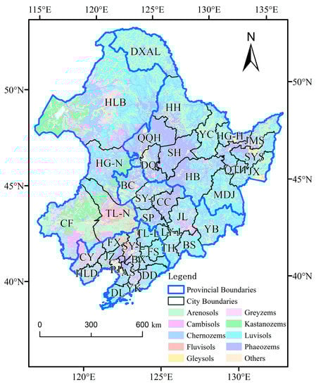
Figure 1.
The geographical location of the study area.
2.2. Indicator System
We selected various indicators from existing studies to assess the ecological safety of CLQ and developed a multilevel indicator model that includes the four levels of socioeconomic drivers, human activity pressure, ecological state, and cultivated land response (DPSR), with a total of fourteen indicators [32,33]. These indicators have been widely used for ecological security assessments and they have strong logical relationships [34,35]. Moreover, we selected indicators with time-series properties to explore the spatiotemporal dynamics of CLQ from 2001 to 2020. The weights of each indicator were calculated using the analytic hierarchy process and the entropy method, and the calculation results passed the test (Table 1).

Table 1.
Indicator information and weights.
2.3. Data Sources
The economic data used in this study were mainly retrieved from provincial statistical yearbooks and the China Statistical Yearbook (accessed on 1 March 2022). Land-use data were obtained from the time-series dataset published by Yang and Huang [36] (https://zenodo.org/record/5210928 (accessed on 1 March 2022)). Meteorological data were retrieved from the precipitation dataset of the Resource and Environment Science and Data Center (https://www.resdc.cn/ (accessed on 1 March 2022)). The maximum synthesis method was used to fuse the normalized difference vegetation index (NDVI) derived from Landsat images from May to September of every year in the study period.
2.4. Improved Matter–Element Model for Early Warning
The matter–element model can describe the quantitative and qualitative changes in indicators and is suitable for multiple indicator assessments [37]. However, in real-world scenarios, the correlation function of the matter–element model needs to be improved and adjusted according to the type of indicator. The CLQ early warning results obtained using the original matter–element model can be significantly unrelated to the actual situation when the effects of positive and negative indicators on early warning are ignored. To address this issue, in this study, we introduced fuzzy sets into the original model, which were used to establish a correlation function of the CLQ early warning model that matches practical applications.
- (1)
- Establish the early warning matter–element of CLQ.
The early warning matter–element of CLQ is represented by an ordered ternary array , where is the level of the early warning, is the indicator feature of the early warning, and is the value of .
- (2)
- Determine the classical and limited fields.
The classical field () indicates the range of values for the city indicator () under different early warning levels. The limited field () indicates the range of values for the city indicator () under all early warning levels.
Here, is the th early warning level, and is the range of values of the th early warning indicator at the th early warning level.
Here, is the total number of early warning levels, and is the range of values of the th indicator.
- (3)
- Establish the correlation function based on fuzzy side distance.
The original matter–element model uses a primary correlation function to calculate the correlation degree (Equation (4)). However, this correlation function ignores the effect of positive and negative indicators of the city’s early warning. For example, the range of the second early warning level of the positive indicator is . Whereas the primary correlation function is used to calculate the correlation degree, it is assumed that when , obtains the maximum value. However, this is inconsistent with the fact that not all indicators achieve the optimal solution at the center point.
Here, is the extensible distance between value of the th indicator and the interval , and and are the range of interval .
To address this issue, in this study, we introduced the fuzzy set to represent the optimal point , with different correlation functions established for positive and negative indicators. The fuzzy side distance correlation function for positive indicators is as follows:
Here, is the right-side distance between and the interval when achieves the optimal solution at . The right-side distance is calculated according to Equation (8).
Here, is the optimal point in interval , and interval ranges from to . In Equation (7), is calculated using the linearly increasing trapezoidal affiliation function (Equation (9)).
Similarly, for the negative indicators, we established a fuzzy side distance correlation function and a calculation function of the left-side distance () and calculated the optimal point () using the linearly decreasing trapezoidal affiliation function.
- (4)
- Calculate the single dominance index.
After defining the fuzzy side distance correlation function, we can calculate the single dominance index () based on the correlation degree (). The dominance index is obtained by normalizing the correlation degree, which makes the matter–element model more objective in representing the early warning results.
- (5)
- Calculate the integrated dominance index.
The indicator weights () are calculated by the entropy method and the analytic hierarchy process. According to the single dominance index (), the integrated dominance index of the th warning level () is calculated according to Equation (14).
2.5. Panel Data Model for Driving Factors of CLQ
Panel data are a type of data with multiple attributes that contain both cross-sectional and time-series information. There are three main types of panel data models—random effects (RE) models, fixed effects (FE) models, and mixed effects (ME) models—that are suitable for analyzing different individual influences [38,39,40]. In this study, we developed a panel data model to investigate the relationship between the dominance index (DI) and different driving factors by considering the time effect and individual effect of early warning targets. Unit root and co-integration tests were performed on the original index data to verify the stationary state and cointegration of the data. Then, we constructed a panel data model to analyze the driving factors of CLQ early warnings.
Here, is the code for warning city ; is time information ; is the integrated dominance index of CLQ; represents the 14 explanatory variables; is the parameter of variable ; and are the intercept terms of the individual effect and the time effect, respectively; and is the random disturbance term.
3. Experiments and Results
3.1. CLQ Early Warning Results
3.1.1. The Classical Field and Limited Field of CLQ
The classical domain () and the nodal domain () are calculated according to Equations (1)–(3) using the integrated weight method and the natural breakpoint method (Table 2). Specifically, in this study, we used all data from 2001 to 2020 to determine the warning thresholds for each indicator based on the median, the mean, and the maximization principle (two-thirds of the total), dividing the warning and no-warning zones (I). We used the natural breakpoint method for more detailed grading, delineating light warnings (II), moderate warnings (III), severe warnings (IV), and extreme warnings (V) for zones with warnings. We took the year 2001 as the baseline to establish a relative risk system, which was used to analyze the secure state of CLQ in the study area. This threshold determination method considers the influence of economic development, land reclamation, human activities, and ecological conditions on the CLQ in the whole region.
Table 2.
The classical field and limited field.
3.1.2. Indicator Levels and Warning Result Levels
As for the positive and negative indicators, the corresponding fuzzy side distance correlation functions were determined, and the dominance index of each indicator was calculated according to Equations (4)–(13). Additionally, each indicator’s early warning level was established according to the maximum affiliation theory, and the unit with the highest dominance index value was determined as the early warning level of the indicator. Then, the integrated dominance index was calculated according to Equation (14) to determine the integrated warning level. The results for the cities in Liaoning Province in 2010 are presented as an example (Table 3) to illustrate the correlation between the indicator level and the integrated warning result level. Table 3 shows that most cities have a no-warning level, but each indicator has a distinct warning level. The integrated warning level in Shenyang is a no warning, but indicators A1, A2, B2, and C2 are extreme warnings. Indicators C1, D2, and D3 in Dalian are no warnings, but the integrated warning level is a moderate warning. Indicators A1, A2, A3, B1, C2, and D1 in Fuxin are light warnings, and the integrated warning level is also a light warning. As a result, each indicator’s warning level has a unique impact on the integrated warning results. The superiority of the performance of the matter–element model lies in its ability to transform the incompatible relationship between multiple indicators into a compatible relationship, showing the correlation between the individual indicator levels and the integrated warning results.
Table 3.
Early warning indicators and results for Liaoning Province in 2010.
3.1.3. CLQ Early Warning Results Based on the Improved Matter–Element Model
An early warning indicator system for CLQ was constructed using 2001 as the base year to analyze changes in CLQ in the black soil region of northeast China from 2001 to 2020; Figure 2 shows the spatial variation of the CLQ early warning. There are now significantly fewer areas in which warnings are present, indicating that CLQ has changed over time to become warning-free. As shown in Figure 2a, the CLQ in the northern part of the black soil region is significantly better than that in the southern part; however, there are still CLQ warnings in nearly half of the cities. In 2005, the warning level clearly decreased in the eastern part of the black soil region, but significant warnings remained in the western part. As shown in Figure 2c,d, most cities have no warnings, and only a few cities have light or moderate warnings. There are no dramatic warnings for the CLQ in 2020, except for a few cities with light or moderate warnings.
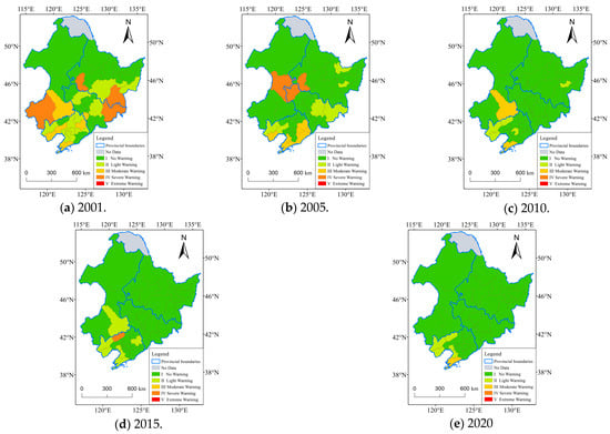
Figure 2.
Spatial distribution of CLQ warning results.
3.2. Spatiotemporal Driving Factors of CLQ
A panel data model was constructed to analyze the driving factors of spatiotemporal variability affecting CLQ (Section 2.5). The early warning integrated dominance index is the explained variable, and the 14 indicators are the explanatory variables. We tested the raw data and the panel data model sequentially by a unit root test, co-integration test, and model test, and then we estimated the parameters. The estimated parameters reflect the correlation between each early warning indicator and the integrated dominance index and indicate whether each indicator has a positive or negative impact on the CLQ early warning results.
3.2.1. Unit Root Test
Stationarity tests of the 14 indicators were performed using Stata software. We performed unit root tests for the explained variable y (the integrated dominance index) and the explanatory variables (A1, A2, A3, A4, B1, B2, B3, C1, C2, C3, D1, D2, D3, and D4) using IPS and HT tests, respectively. As shown in Table 4, variables y, A4, B1, C1, C3, and D4 are stationary. Although variables A1, A2, A3, B2, B3, C2, D1, D2, and D3 are non-stationary, their first-order difference results are stationary.
Table 4.
The results of the unit root test.
3.2.2. Cointegration Test
Because a portion of the raw data is non-stationary, which can lead to pseudo-regression errors in the regression results, it was necessary to perform cointegration tests to eliminate the negative effects of the data. Therefore, we took the raw data of all variables and the raw data of some variables (stationary state) with the first-order difference data of other variables (non-stationary state) as the input data to perform two co-integration tests. As shown in Table 5, the raw and first-order difference data of the explanatory variables were all co-integrated with the explained variable in both experiments.
Table 5.
The result of the cointegration test.
3.2.3. Panel Data Model Test
In this study, the F test, FM test, and Hauman test were used to test different types of panel models (Table 6). The test results indicate that all tests are significant at the 1% level, leading to the rejection of the null hypothesis. In the two experiments, we obtained the consistent conclusion that the FE model outperforms the ME model, the RE model outperforms the ME model, and the FE model outperforms the RE model after the F test, FM test, and Hauman test. Therefore, the FE model was used to analyze the significant relationship between the explanatory and explained variables.
Table 6.
The results of the panel data model test.
3.2.4. Regression Results of the Panel Data Models
Two sets of experiments were performed to confirm the impacts of data stationarity and co-integration on the outcomes of regression analysis. In one set of experiments (Table 7, Part 1), we performed a regression analysis using raw data for all variables. In another set of experiments (Part 2), we used raw data for some variables (stationary state) and first-order difference variables for others (non-stationary state) as the input data. The FE model in the Part 2 experiment was determined to be the final panel data model suitable for the analysis of the spatiotemporal driving factors of CLQ. As shown in Table 7, because the unit root and cointegration tests were not performed in the Part 1 experiment, more explanatory variables were significantly correlated with the explained variables because more explanatory factors were misfit with the explained variables due to the pseudo-regression phenomena. The regression results of the FE model in the Part 2 experiment show that five explaining variables (A4, B2, C1, C3, and D4) were significantly correlated with the explained variables. One explanatory variable (B2) was significantly and negatively correlated with the CLQ warning results. Variable B2 (land carrying capacity) indicates the population density of each city. The more people there are in a specific land area, the more pressure there is on the environment, and the more the CLQ is affected. Four explanatory variables (A4, C1, C3, and D4) were significantly and positively correlated with the CLQ warning results. Variable A4 (agricultural GDP growth rate) indicates the state of agricultural economic development, which has a potential impact on improvements in the CLQ. Variable C1 (annual precipitation) primarily functions in the grain-growing period. A high value of variable C3 (habitat quality index) implies a healthy ecological environment, which benefits the CLQ. In addition to being essential for food security, variable D4 (grain yield per unit of cultivated land area) serves as a critical indicator of the CLQ.
Table 7.
Regression results of the different panel data models.
4. Discussion
The black soil region of northeast China is a crucial grain-producing region, and its CLQ trend directly affects national food security [41]. Socioeconomic development in the last 20 years has contributed to improvements in the ecological environment of the arable land, which have a potential influence on the ecological safety of CLQ [42,43]. In 2001, the northern portion of the black soil region had better CLQ than the southern portion, with Chifeng, Daqing, Mudanjiang, and Yanbian under severe warnings. This phenomenon can be attributed to the fact that these cities are in a state of high urbanization, with a concentrated urban population, underutilization of arable land, and a decline in rural population. There is a correlation between the urbanization rate and the CLQ [44]. With the development of society and the implementation of policies related to cultivated land protection, arable land has been effectively protected and appropriately utilized in the black soil region, which plays an essential role in improving food production, protecting cultivated land security, and maintaining ecological health [45]. Table 8 shows the statistical results for the different warning levels between 2001 and 2020. Among them, extreme warnings only account for 0.13%. The results of this study demonstrate that most cities in northeast China were in a secure state in 2020 (Table 8), indicating that the improvements in the CLQ and the ecological preservation of cultivated land both significantly benefited from socioeconomic development.
Table 8.
Statistical analysis of CLQ warning results.
In this study, we divided CLQ changes into three types—stable, gradual, and abrupt—to analyze the trends in CLQ changes over the previous 20 years. We developed classification guidelines by statistically analyzing the CLQ in 39 cities, as shown in Table 9. An abrupt change indicates that a city’s CLQ early warning level experienced a dramatic increase or decrease in the past 20 years. This type of change requires the attention of government departments, including an analysis of the current status of CLQ in the city and prompt identifications of possible safety hazards. A gradual change indicates a continuous increase or decrease in a city’s CLQ early warning level over time. It is essential to focus on the ongoing decline and the factors that may contribute to the degradation of CLQ. A stable change indicates that a city’s CLQ has been in a stationary state; cities of this type are in an almost warning-free state. This classification method has an essential guiding role in CLQ monitoring and early warning, providing scientific decision-making support for black soil conservation and utilization by indicating the degree to which attention should be paid to areas with varying change tendencies.
Table 9.
Principles of classification of the types of changes in CLQ.
The results of the panel data model show (Table 7) that the primary driving factors of CLQ are agricultural GDP growth rate, land carrying capacity, grain yield per unit of cultivated land area, annual precipitation, and habitat quality index. These results indicate that the index system established in this study can scientifically provide early warning results for CLQ, taking into account four dimensions: socioeconomic development, human–land relationships, ecological environment, and cultivated land characteristics [46,47]. The development of appropriate political, technical, and management strategies can mobilize farmers’ willingness to produce to attain higher incomes. However, these strategies must be based on the appropriate exploitation of cultivated land [48]. A high-quality tillage layer and management strategy can contribute significantly to improvements in CLQ [49,50]. Continued population growth and human activity put varying degrees of external pressure on cultivated land, increasing the demand for multiple agricultural products [51,52,53]. The overutilization of cropland can also damage its health and lead to a decline in its quality [54,55]. An increase in grain yield indicates an improvement in the cropland’s productivity, which is also influenced by other factors, such as cultivated land conditions, cultivated land fragmentation, the application of chemical fertilizers, and conservation policies [56,57,58]. As a result, an increase in grain yield does not entirely reflect an improvement in the CLQ, but it is undeniable that grain yield is an essential sign of the CLQ state [59]. The rainy season in northeast China is concentrated in the summer; these conditions of high temperatures, rainfall, and long periods of sunshine are favorable for crop growth [60,61]. Therefore, rainfall showed a significant positive effect on the CLQ. The habitat quality index considers the influence of nearby land-use types on arable land, serving as a characterization indicator of habitat quality. In addition to reflecting regional biodiversity, it also illustrates the impact of various habitat threats and disturbances on CLQ.
5. Conclusions
Timely monitoring and accurate early CLQ warnings are essential for cultivated land safety. In this study, we constructed a DPSR model to select indicators covering four dimensions: socioeconomic drivers, human activity pressure, ecological state, and cultivated land response. We introduced fuzzy sets into the matter–element model to construct a fuzzy side distance-based matter–element model for CLQ assessment and early warning. The experimental results in the black soil region of northeast China from 2001 to 2020 validate the applicability of the optimized matter–element model for ecological safety assessments and CLQ early warning. In the past two decades, socioeconomic development has effectively improved the ecological safety of CLQ. Compared to 2001, Dalian, Yingkou, Fuxin, Panjin, Chaoyang, and Huludao had an early warning situation for CLQ in 2020. Specifically, Yingkou, Fuxin, Panjin, Chaoyang, and Huludao are under light warnings, and Dalian is under a moderate warning. In the whole region, the CLQ is the best in Heilongjiang Province and the worst in Liaoning Province. This result implies that rapid socioeconomic development positively affects CLQ. To better understand the key variables influencing CLQ, a panel data model was constructed to analyze the critical spatiotemporal drivers of CLQ. The experimental results demonstrate that the developments of the agricultural economy, human activities, grain yield, precipitation, and habitat quality were significant driving factors in changes in CLQ. The analysis results reported in this study provide a scientific basis for regional CLQ assessment and early warning.
However, due to the limitations of experimental conditions and difficulties in obtaining data, we did not use natural soil conditions and profile data in this study to assess the ecological safety of cropland quality. Time-series soil profile data, especially for soil natural conditions, physical properties, and chemical properties, are difficult to obtain. This is a challenging task, because such data require annual monitoring and specialized equipment. In region-scale areas, it is even more difficult to obtain such data accurately.
Author Contributions
Conceptualization, methodology, data curation, writing—original draft preparation, Z.L.; funding acquisition, project administration, writing—review and editing, M.W.; conceptualization, visualization, X.L. (Xingnan Liu); writing—review and editing, F.W.; investigation, writing—review and editing, X.L. (Xiaoyan Li); investigation, writing—review and editing, G.H.; conceptualization, writing—review and editing, J.W.; resources, S.Z. All authors have read and agreed to the published version of the manuscript.
Funding
This research work was financially supported by the National Key R&D Program of China (No.2021YFD1500104-4), the Technological Basic Research Program of China (2021FY100406), and the Natural Science Foundation of Jilin province (No.20210101098JC).
Data Availability Statement
Not applicable.
Conflicts of Interest
The authors declare no conflict of interest.
Appendix A
The study area consists of Jilin Province, Liaoning Province, Heilongjiang Province, and four cities in the eastern Inner Mongolia Autonomous Region (Figure 1). Jilin Province includes Baishan City (BS), Baicheng City (BC), Changchun City (CC), Jilin City (JL), Liaoyuan City (LY-J), Siping City (SP), Songyuan City (SY-J), Tonghua City (TH), and Yanbian Korean Autonomous Prefecture (YB). Liaoning Province includes Anshan City (AS), Benxi City (BX), Chaoyang City (CY), Dandong City (DD), Dalian City (DL), Fushun City (FS), Fuxin City (FX), Huludao City (HLD), Jinzhou City (JZ), Liaoyang City (LY-L), Panjin City (PJ), Shenyang City (SY-L), Tongliao City (TL-L), and Yingkou City (YK). Heilongjiang Province includes Daqing City (DQ), Daxinganling Region (DXAL), Harbin City (HB), Hegang City (HG-H), Heihe City (HH), Jiamusi City (JMS), Jixi City (JX), Mudanjiang City (MDJ), Qiqihar City (QQH), Qitaihe City (QTH), Suihua City (SH), Shuangyashan City (SYS), and Yichun City (YC). The four cities in the eastern Inner Mongolia Autonomous Region are Chifeng City (CF), Hinggan League (HG-N), Hulunbuir City (HLB), and Tongliao City (TL-N).
References
- Mirghaed, F.A.; Souri, B. Spatial analysis of soil quality through landscape patterns in the Shoor River Basin, Southwestern Iran. Catena 2022, 211, 106028. [Google Scholar] [CrossRef]
- Yang, X.; Zhou, X.H.; Shang, G.Y.; Zhang, A.L. An evaluation on farmland ecological service in Jianghan Plain, China-from farmers’ heterogeneous preference perspective. Ecol. Indic. 2022, 136, 108665. [Google Scholar] [CrossRef]
- Li, Q.F.; Guo, W.H.; Sun, X.B.; Yang, A.Z.; Qu, S.J.; Chi, W.F. The Differentiation in Cultivated Land Quality between Modern Agricultural Areas and Traditional Agricultural Areas: Evidence from Northeast China. Land 2021, 10, 842. [Google Scholar] [CrossRef]
- Teng, Y.; Pang, B.Y.; Guo, X.Y. Study on the quality improvement on black land in Northeast China under the environment of sustainable agricultural development. Kybernetes 2021, 52, 809–827. [Google Scholar] [CrossRef]
- Zhou, J.; Guan, D.W.; Zhou, B.K.; Zhao, B.S.; Ma, M.C.; Qin, J.; Jiang, X.; Chen, S.F.; Cao, F.M.; Shen, D.L.; et al. Influence of 34-years of fertilization on bacterial communities in an intensively cultivated black soil in northeast China. Soil Biol. Biochem. 2015, 90, 42–51. [Google Scholar] [CrossRef]
- Wei, J.B.; Xiao, D.N.; Zhang, X.Y.; Li, X.Y. Topography and land use effects on the spatial variation of soil organic carbon: A case study in a typical small watershed of the black soil region in northeast China. Eurasian Soil Sci. 2011, 41, 39–47. [Google Scholar] [CrossRef]
- Zhang, S.X.; Li, Q.; Zhang, X.P.; Wei, K.; Chen, L.J.; Liang, W.J. Effects of conservation tillage on soil aggregation and aggregate binding agents in black soil of Northeast China. Soil Tillage Res. 2012, 124, 196–202. [Google Scholar] [CrossRef]
- Everest, T.; Savaskan, G.S.; Or, A.; Ozcan, H. Suitable site selection by using full consistency method (FUCOM): A case study for maize cultivation in northwest Turkey. Environ. Dev. Sustain. 2022, 1–20. [Google Scholar] [CrossRef]
- Song, W.; Zhang, H.; Zhao, R.; Wu, K.; Li, X.; Niu, B.; Li, J. Study on cultivated land quality evaluation from the perspective of farmland ecosystems. Ecol. Indic. 2022, 139, 108959. [Google Scholar] [CrossRef]
- Zou, S.J.; Zhang, L.; Huang, X.; Osei, F.B.; Ou, G.L. Early ecological security warning of cultivated lands using RF-MLP integration model: A case study on China’s main grain-producing areas. Ecol. Indic. 2022, 141, 109059. [Google Scholar] [CrossRef]
- Kong, X. China must protect high-quality arable land. Nature 2014, 506, 7. [Google Scholar] [CrossRef] [PubMed]
- Wu, Y.Z.; Shan, L.P.; Guo, Z.; Peng, Y. Cultivated land protection policies in China facing 2030: Dynamic balance system versus basic farmland zoning. Habitat Int. 2017, 69, 126–138. [Google Scholar] [CrossRef]
- Berrouet, L.M.; Machado, J.; Villegas-Palacio, C. Vulnerability of socio—Ecological systems: A conceptual Framework. Ecol. Indic. 2018, 84, 632–647. [Google Scholar] [CrossRef]
- Ma, T.Y.; Li, J.; Bai, S.; Chang, F.Z.; Jiang, Z.; Yan, X.G.; Shao, J.H. Optimization and Construction of Ecological Security Patterns Based on Natural and Cultivated Land Disturbance. Sustainability 2022, 14, 16501. [Google Scholar] [CrossRef]
- Li, W.; Wang, D.; Li, Y.; Zhu, Y.; Wang, J.; Ma, J. A multi-faceted, location-specific assessment of land degradation threats to peri-urban agriculture at a traditional grain base in northeastern China. J. Environ. Manag. 2020, 271, 111000. [Google Scholar] [CrossRef]
- Song, W.; Pijanowski, B.C. The effects of China’s cultivated land balance program on potential land productivity at a national scale. Appl. Geogr. 2014, 46, 158–170. [Google Scholar] [CrossRef]
- Yang, X.; Shang, G. Smallholders’ Agricultural Production Efficiency of Conservation Tillage in Jianghan Plain, China-Based on a Three-Stage DEA Model. Int. J. Environ. Res. Public Health 2020, 17, 7470. [Google Scholar] [CrossRef]
- Pardini, G.; Gispert, M.; Emran, M.; Doni, S. Rainfall/runoff/erosion relationships and soil properties survey in abandoned shallow soils of NE Spain. J. Soils Sediments 2016, 17, 499–514. [Google Scholar] [CrossRef]
- Liu, T.J.; Xu, X.T.; Yang, J. Experimental study on the effect of freezing-thawing cycles on wind erosion of black soil in Northeast China. Cold Reg. Sci. Technol. 2017, 136, 1–8. [Google Scholar] [CrossRef]
- Everest, B. Farmers’ adaptations of soil and water conservation in mitigating climate change. Arab. J. Geosci. 2021, 14, 2141. [Google Scholar] [CrossRef]
- Walz, R. Development of Environmental Indicator Systems: Experiences from Germany. Environ. Manag. 2000, 25, 613–623. [Google Scholar] [CrossRef]
- Hu, X.J.; Ma, C.M.; Huang, P.; Guo, X. Ecological vulnerability assessment based on AHP-PSR method and analysis of its single parameter sensitivity and spatial autocorrelation for ecological protection—A case of Weifang City, China. Ecol. Indic. 2021, 125, 107464. [Google Scholar] [CrossRef]
- Chen, G.Q.; Han, M.Y. Virtual land use change in China 2002–2010: Internal transition and trade imbalance. Land Use Policy 2015, 47, 55–65. [Google Scholar] [CrossRef]
- Cai, W. Matter-Element and Application; Science and Technology Literature Publishing House: Beijing, China, 1994. [Google Scholar]
- Pan, G.; Xu, Y.; Yu, Z.; Song, S.; Zhang, Y. Analysis of river health variation under the background of urbanization based on entropy weight and matter-element model: A case study in Huzhou City in the Yangtze River Delta, China. Environ. Res. 2015, 139, 31–35. [Google Scholar] [CrossRef]
- He, Y.X.; Dai, A.Y.; Zhu, J.A.; He, H.Y.; Li, F.R. Risk assessment of urban network planning in china based on the matter-element model and extension analysis. Int. J. Electr. Power Energy Syst. 2011, 33, 775–782. [Google Scholar] [CrossRef]
- Gong, J.Z.; Liu, Y.S.; Chen, W.L. Land suitability evaluation for development using a matter-element model: A case study in Zengcheng, Guangzhou, China. Land Use Policy 2012, 29, 464–472. [Google Scholar] [CrossRef]
- Deng, X.J.; Xu, Y.P.; Han, L.F.; Yu, Z.H.; Yang, M.N.; Pan, G.B. Assessment of river health based on an improved entropy-based fuzzy matter-element model in the Taihu Plain, China. Ecol. Indic. 2015, 57, 85–95. [Google Scholar] [CrossRef]
- Li, B.; Yang, G.; Wan, R.; Hormann, G. Dynamic water quality evaluation based on fuzzy matter-element model and functional data analysis, a case study in Poyang Lake. Environ. Sci. Pollut. Res. 2017, 24, 19138–19148. [Google Scholar] [CrossRef] [PubMed]
- Shi, Y.Y.; Duan, W.K.; Fleskens, L.; Li, M.; Hao, J.M. Study on evaluation of regional cultivated land quality based on resource-asset-capital attributes and its spatial mechanism. Appl. Geogr. 2020, 125, 102284. [Google Scholar] [CrossRef]
- Derakhshan-Babaei, F.; Nosrati, K.; Mirghaed, F.A.; Egli, M. The interrelation between landform, land-use, erosion and soil quality in the Kan catchment of the Tehran province, central Iran. Catena 2021, 204, 105412. [Google Scholar] [CrossRef]
- Li, W.B.; Wang, D.Y.; Li, H.; Liu, S.H. Urbanization-induced site condition changes of peri-urban cultivated land in the black soil region of northeast China. Ecol. Indic. 2017, 80, 215–223. [Google Scholar] [CrossRef]
- Su, M.; Guo, R.Z.; Hong, W.Y. Institutional transition transition and implementation path for cultivated land protection in highly urbanized regions: A case study of Shenzhen, China. Land Use Policy 2019, 81, 493–501. [Google Scholar] [CrossRef]
- Shi, Q.L.; Lin, Y.Z.; Zhang, E.P.; Yan, H.M.; Zhan, J.Y. Impacts of Cultivated Land Reclamation on the Climate and Grain Production in Northeast China in the Future 30 Years. Adv. Meteorol. 2013, 2013, 1–8. [Google Scholar] [CrossRef]
- Fan, R.Q.; Zhang, X.P.; Yang, X.M.; Liang, A.Z.; Jia, S.X.; Chen, X.W. Effects of tillage management on infiltration and preferential flow in a black soil, Northeast China. Chin. Geogr. Sci. 2013, 23, 312–320. [Google Scholar] [CrossRef]
- Yang, J.; Huang, X. The 30 m annual land cover dataset and its dynamics in China from 1990 to 2019. Earth Syst. Sci. Data 2021, 13, 3907–3925. [Google Scholar] [CrossRef]
- Yang, Q.; Lin, A.W.; Zhao, Z.Z.; Zou, L.; Sun, C. Assessment of Urban Ecosystem Health Based on Entropy Weight Extension Decision Model in Urban Agglomeration. Sustainability 2016, 8, 869. [Google Scholar] [CrossRef]
- Deng, X.Z.; Huang, J.K.; Rozelle, S.; Uchida, E. Growth, population and industrialization, and urban land expansion of China. J. Urban Econ. 2008, 63, 96–115. [Google Scholar] [CrossRef]
- Zhang, C.G.; Lin, Y. Panel estimation for urbanization, energy consumption and CO2 emissions: A regional analysis in China. Energy Policy 2012, 49, 488–498. [Google Scholar] [CrossRef]
- Cheng, Z.H.; Li, L.S.; Liu, J. Identifying the spatial effects and driving factors of urban PM2.5 pollution in China. Ecol. Indic. 2017, 82, 61–75. [Google Scholar] [CrossRef]
- Germer, J.; Sauerborn, J.; Asch, F.; de Boer, J.; Schreiber, J.; Weber, G.; Muller, J. Skyfarming an ecological innovation to enhance global food security. J. Verbrauch. Lebensm.-J. Consum. Prot. Food Saf. 2011, 6, 237–251. [Google Scholar] [CrossRef]
- Xie, H.; He, Y.; Choi, Y.; Chen, Q.; Cheng, H. Warning of negative effects of land-use changes on ecological security based on GIS. Sci. Total Environ. 2020, 704, 135427. [Google Scholar] [CrossRef]
- Liu, X.; Shi, L.J.; Qian, H.Y.; Sun, S.K.; Wu, P.T.; Zhao, X.N.; Engel, B.A.; Wang, Y.B. New problems of food security in Northwest China: A sustainability perspective. Land Degrad. Dev. 2020, 31, 975–989. [Google Scholar] [CrossRef]
- Wang, H.; Zhu, Y.; Wang, J.; Han, H.; Niu, J.; Chen, X. Modeling of spatial pattern and influencing factors of cultivated land quality in Henan Province based on spatial big data. PLoS ONE 2022, 17, e0265613. [Google Scholar] [CrossRef] [PubMed]
- Liu, S.H.; Wang, D.Y.; Li, H.; Li, W.B.; Wang, Q. Ecological Land Fragmentation Evaluation and Dynamic Change of a Typical Black Soil Farming Area in Northeast China. Sustainability 2017, 9, 300. [Google Scholar] [CrossRef]
- Liu, Y.; Li, J.; Liu, C.; Wei, J. Evaluation of cultivated land quality using attention mechanism-back propagation neural network. PeerJ Comput. Sci. 2022, 8, e948. [Google Scholar] [CrossRef] [PubMed]
- Liang, J.; Zheng, H.; Cai, Z.; Zhou, Y.; Xu, Y. Evaluation of Cultivated Land Quality in Semiarid Sandy Areas: A Case Study of the Horqin Zuoyihou Banner. Land 2022, 11, 1457. [Google Scholar] [CrossRef]
- Song, W.; Wu, K.; Zhao, H.; Zhao, R.; Li, T. Arrangement of High-standard Basic Farmland Construction Based on Village-region Cultivated Land Quality Uniformity. Chin. Geogr. Sci. 2018, 29, 325–340. [Google Scholar] [CrossRef]
- Kang, L.; Zhao, R.; Wu, K.N.; Huang, Q.; Zhang, S.C. Impacts of Farming Layer Constructions on Cultivated Land Quality under the Cultivated Land Balance Policy. Agronomy 2021, 11, 2403. [Google Scholar] [CrossRef]
- Sheng, Y.; Liu, W.; Xu, H.; Gao, X. The Spatial Distribution Characteristics of the Cultivated Land Quality in the Diluvial Fan Terrain of the Arid Region: A Case Study of Jimsar County, Xinjiang, China. Land 2021, 10, 896. [Google Scholar] [CrossRef]
- Wang, L.Y.; Anna, H.; Zhang, L.Y.; Xiao, Y.; Wang, Y.Q.; Xiao, Y.; Liu, J.G.; Ouyang, Z.Y. Spatial and Temporal Changes of Arable Land Driven by Urbanization and Ecological Restoration in China. Chin. Geogr. Sci. 2019, 29, 809–819. [Google Scholar] [CrossRef]
- Gong, H.; Zhao, Z.; Chang, L.; Li, G.; Li, Y.; Li, Y. Spatiotemporal Patterns in and Key Influences on Cultivated-Land Multi-Functionality in Northeast China’s Black-Soil Region. Land 2022, 11, 1101. [Google Scholar] [CrossRef]
- Chen, Y.; Wang, S.; Wang, Y. Spatiotemporal Evolution of Cultivated Land Non-Agriculturalization and Its Drivers in Typical Areas of Southwest China from 2000 to 2020. Remote Sens. 2022, 14, 3211. [Google Scholar] [CrossRef]
- Yu, D.; Wang, D.Y.; Li, W.B.; Liu, S.H.; Zhu, Y.L.; Wu, W.J.; Zhou, Y.H. Decreased Landscape Ecological Security of Peri-Urban Cultivated Land Following Rapid Urbanization: An Impediment to Sustainable Agriculture. Sustainability 2018, 10, 394. [Google Scholar] [CrossRef]
- Cui, H.J.; Guo, P.; Li, M.; Guo, S.S.; Zhang, F. A multi-risk assessment framework for agricultural land use optimization. Stoch. Environ. Res. Risk Assess. 2018, 33, 563–579. [Google Scholar] [CrossRef]
- Duan, X.W.; Xie, Y.; Feng, Y.J.; Yin, S.Q. Study on the Method of Soil Productivity Assessment in Black Soil Region of Northeast China. Agric. Sci. China 2009, 8, 472–481. [Google Scholar] [CrossRef]
- Qian, F.; Chi, Y.; Lal, R.; Lorenz, K. Spatio-temporal characteristics of cultivated land fragmentation in different landform areas with a case study in Northeast China. Ecosyst. Health Sustain. 2020, 6, 1800415. [Google Scholar] [CrossRef]
- Li, D.; Zhai, Y.; Lei, Y.; Li, J.; Teng, Y.; Lu, H.; Xia, X.; Yue, W.; Yang, J. Spatiotemporal evolution of groundwater nitrate nitrogen levels and potential human health risks in the Songnen Plain, Northeast China. Ecotoxicol. Environ. Saf. 2021, 208, 111524. [Google Scholar] [CrossRef]
- Lu, Z.-J.; Song, Q.; Liu, K.-B.; Wu, W.-B.; Liu, Y.-X.; Xin, R.; Zhang, D.-M. Rice cultivation changes and its relationships with geographical factors in Heilongjiang Province, China. J. Integr. Agric. 2017, 16, 2274–2282. [Google Scholar] [CrossRef]
- Li, Z.G.; Tang, H.J.; Yang, P.; Wu, W.B.; Chen, Z.X.; Zhou, Q.B.; Zhang, L.; Zou, J.Q. Spatio-temporal responses of cropland phenophases to climate change in Northeast China. J. Geogr. Sci. 2012, 22, 29–45. [Google Scholar] [CrossRef]
- Yang, X.; Lin, E.; Ma, S.M.; Ju, H.; Guo, L.P.; Xiong, W.; Li, Y.; Xu, Y.L. Adaptation of agriculture to warming in Northeast China. Clim. Chang. 2007, 84, 45–58. [Google Scholar] [CrossRef]
Disclaimer/Publisher’s Note: The statements, opinions and data contained in all publications are solely those of the individual author(s) and contributor(s) and not of MDPI and/or the editor(s). MDPI and/or the editor(s) disclaim responsibility for any injury to people or property resulting from any ideas, methods, instructions or products referred to in the content. |
© 2023 by the authors. Licensee MDPI, Basel, Switzerland. This article is an open access article distributed under the terms and conditions of the Creative Commons Attribution (CC BY) license (https://creativecommons.org/licenses/by/4.0/).