Abstract
In order to ensure the sustainability of production from agricultural lands, the degradation processes surrounding the fertile land environment must be monitored. Human-induced risk and status of soil degradation (SD) were assessed in the Northern-Eastern part of the Nile delta using trend analyses for years 2013 to 2023. SD hotspot areas were identified using time-series analysis of satellite-derived indices as a small fraction of the difference between the observed indices and the geostatistical analyses projected from the soil data. The method operated on the assumption that the negative trend of photosynthetic capacity of plants is an indicator of SD independently of climate variability. Combinations of soil, water, and vegetation’s indices were integrated to achieve the goals of the study. Thirteen soil profiles were dug in the hotspots areas. The soil was affected by salinity and alkalinity risks ranging from slight to strong, while compaction and waterlogging ranged from slight to moderate. According to the GIS-model results, 30% of the soils were subject to slight degradation threats, 50% were subject to strong risks, and 20% were subject to moderate risks. The primary human-caused sources of SD are excessive irrigation, poor conservation practices, improper utilisation of heavy machines, and insufficient drainage. Electrical conductivity (EC), exchangeable soil percentage (ESP), bulk density (BD), and water table depth were the main causes of SD in the area. Generally, chemical degradation risks were low, while physical risks were very high in the area. Trend analyses of remote sensing indices (RSI) proved to be effective and accurate tools to monitor environmental dynamic changes. Principal components analyses were used to compare and prioritise among the used RSI. RSI pixel-wise residual trend indicated SD areas were related to soil data. The spatial and temporal trends of the indices in the region followed the patterns of drought, salinity, soil moisture, and the difficulties in separating the impacts of drought and submerged on SD on vegetation photosynthetic capacity. Therefore, future studies of land degradation and desertification should proceed using indices as a factor predictor of SD analysis.
1. Introduction
One of the most important reliable collections of information in any environmental or development program at the national or international level is the collected details of SD processes [1]. This is due to the negative effects that these processes have on ecosystem stability, which ultimately leads to a decline in land services [2]. SD frequently threatens the livelihoods of poor rural people in developing countries, particularly those in low- and middle-income countries [3,4,5,6,7,8], where it constitutes a gradual deterioration in the agricultural sector and causes a weakening of the ability of the soil to produce biomass for humans and animals [9]. Thus, SD represents a clear and direct threat to food security. In addition, its aggravation may eventually lead to the abandonment of the soil [10]. SD requires exorbitant costs, time, experience, and effort, because it is often the result of extensive changes in soil properties. It is a complex phenomenon that results from natural and/or human factors [11]. The failure to implement an efficient framework of sustainable agriculture, as well as illiteracy, inexperience, and overuse of the land, all contribute to the condition of soil degradation [12]. Soil degradation takes place when the soil quality deteriorates both onsite and offsite, where the processes contribute to the harmful effects of nature’s physical (compression, waterlogging, sealing, and crusting of topsoil), chemical (salinisation, alkalisation, acidification, and nutrient degradation), and/or biological (loss of organic matter, land cover, and biodiversity) elements. Natural degradation risks are dimensions of existing and projected soil productivity deriving mostly from natural variables such as terrain, soils, and climate, rather than human intervention.
Monitoring the SD process over a specified period requires the implementation of geomatics applications for a better use of historical RS data. This helps detect SD and recognise its different types. Practical measurement using RS techniques helps identify and maintain indicators of soil health. RS has been used in SD studies for acquiring input data for SD calculations, for an indirect assessment of SD using the analysis of vegetation cover, and for a direct identification of SD features and SD stages [4,6,7,8,10,11]. Pixel values are directly mapped to color map values in an index image. This equivalent value is used as an index within the map to determine the color of each image pixel. It could be used as direct and/or indirect measurement for soil/vegetation status and/or properties. Through the study of multi- and/or hyperspectral picture bands, remote sensing indices (RSI) for soil, water, and vegetation enable the capture of ecological data from satellites. Light reflection varies depending on the type of plant, the soil, the water content, and other elements. As a result, the spectral reflectance responses shown in satellite data can depict how various electromagnetic waves interact with various features [13,14]. Additionally, these indices are employed to raise the precision of categorisation algorithms. Indices improve spectral information and make it easier to distinguish between different classes of interest. All these elements contribute to an improvement in the mapping of land use and land cover (LULC) [15]. Indices serve two purposes: they provide information about the health and growth of plants, and they assist in classifying various types of land (mining, forest, bare soil, pasture, water surfaces, industrial, etc.). Additionally, certain combinations of vegetation indices boost some crops’ spectral traits while inhibiting others [16]. The wide use of RS imagery for monitoring land and environmental changes was proofed for soil sealing [17,18,19], human or natural factors that cause the loss of forests [20,21,22], effects of global warming [23,24], a wildfire’s damage [25,26], and additional human-made and natural dynamics. Particularly for SD investigations, which are frequently thought of as being over a lengthy period of time, data acquisition costs and time of coverage are the main limits of observation data such as SPOT [27,28] and Sentinel-2 [29,30]. Commercial satellites are expensive per scene compared to the income of developing nations. Only since 2015 has fine resolution, freely accessible data been made available, such as those from the Sentinel mission. Due to the fact that Landsat data (i.e., 4, 5, 7-ETM, and 8-OLI) span approximately 50 years in a row, they are frequently employed in much research across the globe [31]. Landsat data are used for monitoring urban growth and surface temperature, a crucial parameter in environmental studies such as physical, chemical, biological, geomorphological and geological dimensions, thanks to its medium multispectral resolution and potent thermal infrared (TIR) sensors [32,33,34,35,36].
The sustainable development of farmland depends on the reliable monitoring of LULC. The LULC’s dynamics have impacts on SD. Accurate classification of urban land covers has been hampered by the existence of bare soil in rural and periurban areas. This is partially due to the similar spectral properties between urban features and bare soil [37]. Since agricultural bare soil is seasonal and urban features are permanent, multitemporal data provide a possible method to detect bare soil. The absence of the rainy season makes it very simple to utilise multitemporal data in the arid region. Therefore, detecting bare soil is not a difficult process. Many spectral indices generated from Landsat have been developed by academics around the world to distinguish between soil, vegetation, and water [7]. A two-, three-, or four-band combined index is typically used to create such indices from different Landsat wavelengths, ranging from visible through near-infrared (NIR) and shortwave infrared (SWIR) wavelengths.
Achieving resilience to land degradation requires the adoption of land management practices sustainable for the ecosystem. The state of soil degradation is more complex in Egypt, not only due to the interaction of the various factors causing land degradation, but also due to the variation in environmental influences that help accelerate these processes, in addition to the human factor. Since SD is one of the observable phenomena that restrict the Nile delta’s current and potential productivity, it must be monitored, and its various types counted, using all available techniques and tools. The evaluation of degradation is the backbone in determining the appropriate preventive measures necessary to maintain soil health and thus achieve the highest return through sustainable land use. Thus, the current research attempts to assess the level of land degradation in a region of the Northern Nile delta.
2. Materials and Methods
2.1. Study Area
Alluvial plain, lacustrine deposits, and coastal plain soils are covered in the study region, which is located in the Northern-Eastern Nile delta (Figure 1) between the longitudes of 31°05′00″ to 31°42′26″ and latitudes of 31°42′24″ to 31°34′06″. According to the climate data, the region experiences a hot, arid summer and a dry, short winter. The average yearly temperature is 20 °C, with minimum and maximum values of 11 and 28 °C, respectively. The largest amount of rainfall per year, which totals 55.0 mm, falls in January. The potential evapotranspiration (PET) is 4 mm day−1. The soil temperature regime is “thermic” while the soil moisture regime is “torric”, according to [38]. The soil samples are randomly distributed in order to cover the study area, as shown in Figure 1.

Figure 1.
Geographical presentation of soil samples distribution along with the study area location.
Figure 2 includes the extracted features of LULC using digital image processing and decision tree classification for the Landsat 2023 imagery. As a final step, accuracy assessment was conducted using field observations and ground truth data gathered from the field survey. Detection tree categorisation was used to categorise the LULC. The objective of image classification is to automatically categorise all the pixels in a multispectral picture into one or more classes or themes. Different features’ spectral reflectance properties exhibit various combinations of digital numbers (commonly known as spectral signatures). A new output image is produced with a specified number of categories or clusters based on these spectral signatures. The data from these groups can then be used to create thematic maps.
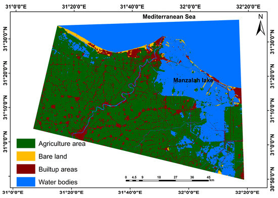
Figure 2.
LULC map of the study area.
Using confusion matrices, accuracy assessment for classification was done in order to show how the reference data are related to the final land cover map. It provided details about oversight mistakes, producer accuracy, commission errors, and user accuracy. The matrix was constructed using 100 examples for each land use category. The following equation was used to determine the overall accuracy percentage:
The obtained overall accuracy is around 94%. The agriculture area, bare land, built-up areas, and water bodies occupy 49, 5, 29, and 17% of the total investigated area, with accuracy assessments of 95, 3, 92, and 97%, respectively. Soil sealing is a major LULC dynamic change in the region.
2.2. Field Work and Laboratory Analysis
To illustrate the various geomorphic units, thirteen soil profiles were dug (Figure 3). The profiles were excavated to a depth of 150 cm, or the depth of the ground water table [39]. This was in addition to collecting 29 surface samples from the areas affected by SD. Both chemical and physical analyses followed the procedures of [40,41].
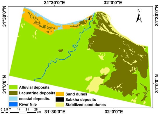
Figure 3.
Geomorphology of the area; it was performed using the overlapping of DEM, Landsat-8, and Geology of Conco [42].
2.3. Assessment of Land Degradation
The evaluation of SD was carried out in accordance with FAO/UNEP and UNESCO [43] and its revision FAO/ISRIC [44]. Using these identifications of remote sensing indices, the risks and types of human-induced land degradation were evaluated. Based on a comparison of the data received from remote sensing indices and the data extracted from soil studies, SD was described.
2.4. GIS Modelling Land Degradation
The following procedures were carried out during the GIS modelling process using ArcGIS: (1) converting the EC, ESP, BD, and water table depth characteristics into raster layers; (2) changing the variables’ classification to the standard scale; (3) providing each variable with a weight; (4) merging and overlaying variables with remote sensing indices; (5) controlling the output value for each cell using conditional tools; and (6) identifying the hotspot areas of SD from the raster dataset.
2.5. Multispectral Satellite Imagery
Landsat-8 was used for the trend analyses of each index applied from 2013 to 2023. The main spectral bands that are relevant to the application of the used indices are Blue, Green, Red, Near-Infrared (NIR), Shortwave Infrared (SWIR) 1, and Shortwave Infrared (SWIR) 2, having spectral resolutions of 0.43–0.45, 0.53–0.59, 0.64–0.67, 0.85–0.88, 1.57–1.65, and 2.11–2.29 µm, respectively, and spatial resolutions of 30 m, as well as Thermal Infrared (TIRS) 1 (spectral resolution of 10.6–11.19 µm) and Thermal Infrared (TIRS) 2 (spectral resolution of 11.50–12.51 µm), having spatial resolutions of 100 m.
Different vegetation indexes (Table 1) are often affected by cloud cover and the shadows of clouds. Different vegetation indexes calculated over pixels containing clouds or shadows will show anomalous values. A quality assessment band accompanied by each date indicates which pixels might be affected by surface conditions (cloud and shadow). Processing steps included the removal of clouds and shadow effects using time series smoothing and quality images.

Table 1.
Remote Sensing Indices (RSI).
- Firstly, 215 datasets covering 10 years of 16 days for different vegetation indexes and quality images were staked.
- For each stacked image, it was possible to search and correct for missing and erroneous data (−9999, 9999). Missing pixel data values were replaced using linear interpolation of neighbouring dates in the time series of each pixel.
- The quality images were used to select dates affected by cloud and shadow for each pixel, and these values were replaced with smoothed time series vectors, by means of Savitzkye-Golay filters with window size 5 and second-order harmonic.
- It was possible to smooth the time series of each pixel by means of Savitzkye-Golay filtering with window size 5 and second-order harmonic, in order to smooth spikes and data outliers.
- Linear regression analysis was performed on the time series of each pixel to derive regression slope values and generate a map of significant trends.
ESPA system bulk ordering was used to download Landsat-8 Collection 2 Surface Reflectance-derived spectral indices in Table 1 from 13 April 2013 to 3 January 2023.
Figure 4 shows the work steps in this research, which began with collecting remote sensing data, then calculating the various indicators and comparing the results with soil analyses and field visits. This process ended with choosing the best combination of indicators for trend analysis in the area.
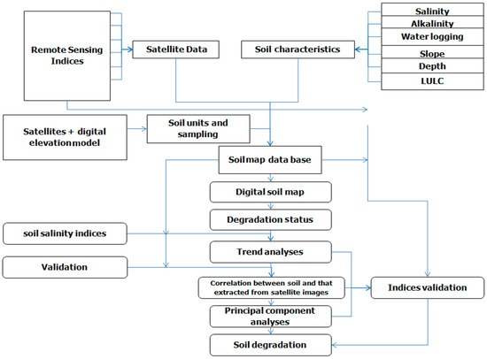
Figure 4.
Flowchart of the work steps.
3. Results
3.1. Soils of the Study Area
The findings show that alluvial soils have very deep soil (>150 cm), while lacustrine soils have soil that is only moderately deep (50–100 cm). They range from being flat to having very slight slopes, with slopes between 0.10 and 1.91%. The soils are neutral, with a pH range of 7.01–8.11 and an EC range of 2.15–6.14 dS m−1, according to [45]. The range of 10.51 to 17.22 g kg−1 for soil organic matter concentration is considered low to moderate [46]. Due to the high levels of clay and organic matter in the soil, the cation exchange capacity (CEC) ranges from high to extremely high [46].
There are none to slight sodicity risks, as shown by the exchangeable sodium percentage (ESP), which ranges from 2.71 to 12.93 [47]. Gypsum and calcium carbonate both have wide ranges of contents, from 4.63 to 8.07 g kg−1 for gypsum and from 3.41 to 12.17 g kg−1 for calcium carbonate. The bulk density of soil varies between 1.11 and 1.47 Mg m−3. The primary soil subgroups, according to [38], are Typic Torrifluvents and Vertic Torrifluvents (Figure 5).
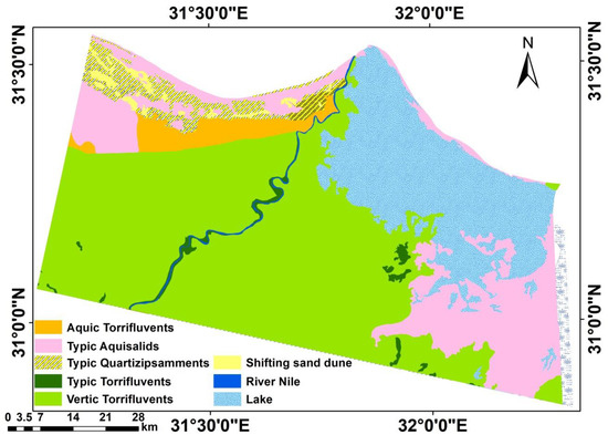
Figure 5.
Soil taxonomy of the study area.
3.2. Human-Induced Soil Degradation
A slight compaction risk exists for soils from alluvial deposits, where soil bulk density (BD) values in practically flat and gradually sloping terrain are 1.21 and 1.28 Mg m−3, respectively. Nevertheless, the EC, ESP, and water table depth (WT) readings are all within the acceptable range. Since the EC, ESP, and Bd values range from 5.47 to 7.56 dS m−1,from 10.22 to 12.78 and from 1.23 to 1.49 Mg m−3, the soils of lacustrine deposits are impacted by moderate salinity, sodicity (alkalinity), and compaction risks. A strong salinity and waterlogging risks have impacts on the soils of coastal deposits (Figure 6).
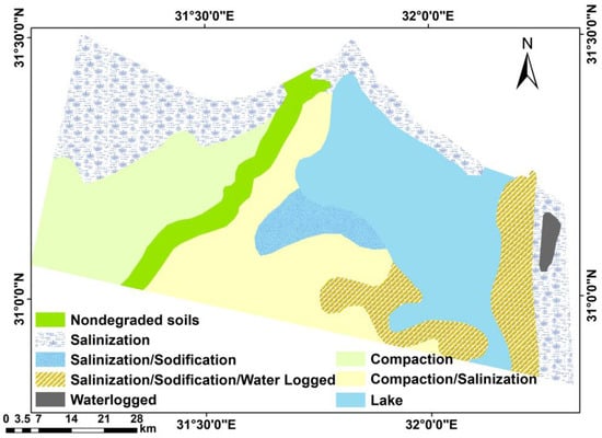
Figure 6.
Degradation risk of the region.
The results of the GIS model reveal three degradation classes; strong, moderate, and slight exist in the studied area. The primary contributing variables to SD in the region are primarily connected to agricultural activities, which are comparable across units. According to [48], excessive irrigation caused by the use of traditional flood irrigation, the lack of conservation measures such as leaching requirements, and the use of brackish water in irrigation due to a lack of fresh water are the main causes of the chemical degradation processes, salinity, and sodicity [49]. Crops are negatively impacted by salinity in a variety of ways, such as decreased water availability due to osmotic effects, particular ion toxicity, and/or nutritional problems. Contrarily, sodicity has a negative impact on the physical properties of the soil, which results in reduced oxygen diffusion and increased soil strength [50]. Soil compaction, one of the two primary types of physical degradation, is primarily brought on by the incorrect use of heavy machinery during tillage and harvest. Due to decreased air and water infiltration and difficulty in allowing roots to penetrate the soil, it deteriorates soil structure [51,52]. Waterlogging is an abiotic stress that alters the soil environment by reducing O2 and increasing CO2, NH3, and C2H4 levels [53]. These modifications lessen root respiration, which hinders root growth and restricts nutrient uptake and transfer to shoots, hence lowering the potential crop production [54]. The main cause of waterlogging in the study area is inadequate drainage.
3.3. Remote Sensing Results from Landsat-8
Several spectral indicators were produced from satellite data (2013–2023), such as the Normalized Difference Vegetation Index (NDVI), Vegetation Condition Index (VCI), Normalized Difference Built-up Index (NDBI), Enhanced Vegetation Index (EVI), Temperature Condition Index (TCI), Crop Water Stress Index (CWSI), Vegetation Health Index (VHI), Soil-Adjusted Vegetation Index (SAVI), Modified Soil Adjusted Vegetation Index (MSAVI), and Normalized Difference Moisture Index (NDMI), which constitute good tools to monitor region status change of land and vegetation cover, water bodies, soil moisture, and soils. It is clear from the results in Figure 6 that there is significant overlap between all the features. This overlap appears clearly between urban areas and bare lands. It represents a technical obstacle in separating the degraded lands and calculating their areas, especially the saline ones. Moreover, the overlap between waterlogged areas, water bodies, and urban areas is an obstacle in separating waterlogged areas (Figure 7 and Figure 8).
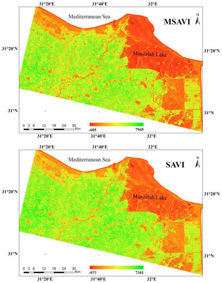
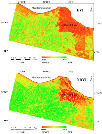
Figure 7.
Remote Sensing Indices (RSI).
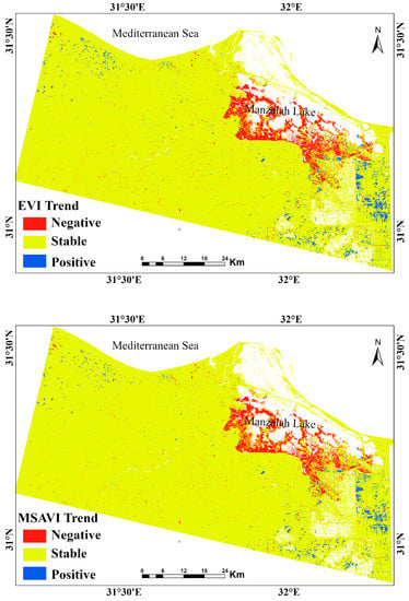
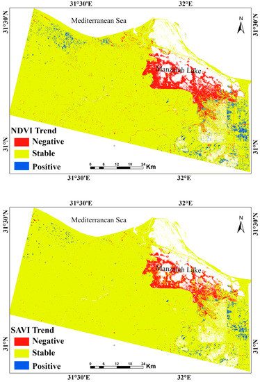
Figure 8.
Trend analyses of Remote Sensing Indices (RSI) in the years from 2013 to 2023.
The residual RSI and its trajectory over time were examined to learn more about the SD process. To find areas with notable negative or positive patterns of the residual RSI, this trend was spatially analysed. In these regions, vegetation photosynthetic variations brought on by variables other than moisture variability are visible. According to the findings, regions that exhibit a negative trend are degraded, whereas locations that exhibit a positive trend are either improved or are not degraded in any capacity.
A mix of degraded and nondegraded patches are frequently visible in the study region, prompting concerns about the consistency of the findings. Figure 7 north, which depicts degradation in the same region but less pronounced than in the east, shows areas with substantial negative trends, or degraded areas, more clearly. A much more reliable and consistent identification of areas that exhibit a pattern in land degradation is made possible by the soil moisture and RSI. SD is not only limited to the coast, but also to wet eastern regions.
The reflectance characteristics of plants, water, and soil were represented by groups of training pixels sets. Studies on bare soil are difficult due to the similarities in the profiles of the two types of cover. The reflectance values of these two features change with visible wavelength, although urban features reflect more energy in this band. Contrarily, bare soil on Landsat-8 reflects more near infrared (0.85–0.88 m) and shortwave infrared 1 (SWIR1: 1.57–1.65 m) wavelengths. In contrast to urban features, bare earth tends to absorb shortwave infrared 2 (SWIR2: 2.11–2.29 m) energy. The combination of NDVI, EVI, SAVI, MSAVI, and NDMI shows the best combination among all indices to recognise the degraded soils in the area.
Figure 6 shows that the primary factor limiting the productivity of an ecosystem is the moisture regime. It is clear from RSI that there are two main explanatory frameworks that are multifaceted for SD accelerations. On the one hand, the region is affected by temperature patterns that accelerate soil salinisation processes, which is evident from the general climate changes. On the other hand, waterlogging in the region can be attributed to the overall changes in the land cover, as well as human intervention in the region and its obvious impact on the land cover in the region. The overall effects of drought have led to widespread soil salinity, particularly in the coastal region. while immersed in the eastern parts led to roasting. However, climate and human actions are important controlling factors that influence the acceleration of SD processes. Therefore, the results indicate that SD is identified as one of the pressing environmental problems in the investigated region which needs great attention to avoid desertification, as it occurs synonymously in all major global drylands. The relationship between soil moisture and vegetation dynamics influences the structure and function of arid and semiarid ecosystems since the development of dryland vegetation is largely dependent on the availability of soil water resources, and irregular patterns of vegetation distribution are usually associated with heterogeneous patterns of soil moisture in regions the roots. Thus, changes in climatic forcing and disturbance regime can lead to a rapid deterioration of vegetation conditions.
4. Discussion
Figure 9 and Figure 10 show the ability of trend analysis to overcome the problem of clouds in the coastal areas and track the condition of the accurate feature, i.e., whether it is negative with an increase in the deterioration speed or positive with a decrease in the deterioration rate or an improved use. It also shows the tracking of areas not affected by changes, especially those resulting from land degradation processes in the region.
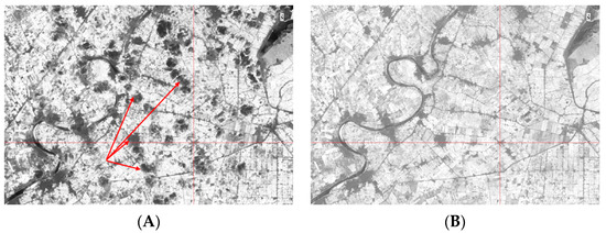
Figure 9.
(A). Clouds before time series processing. (B). Clouds after time series processing.
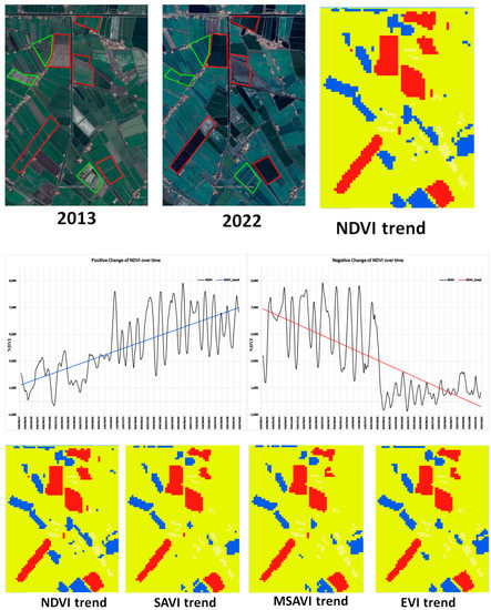
Figure 10.
Negative and positive object detection using trend analyses.
The trend analyses help overcome the clouds obstacles of optical data monitoring objects.
Both soil moisture and drought have been taken into account when adjusting regions with positive and negative patterns in vegetation productivity. When compared to soil data, RSI trend concordance plainly demonstrates SD areas. When compared to regions with significant negative trends based on soil moisture, areas with significant negative trends based on vegetation indices at 95% significant level were also found to be relatively negative. The RSI shows a positive tendency when compared to soil data when the distribution of positive and negative trends is examined. Vegetation indexes and soil moisture distribution both exhibit a largely positive tendency. On the other side, the salinity indices overwhelmingly display a positive tendency. This suggests that drought and soil moisture have a great impact on SD processes.
The majority of the energy from the visible to the infrared spectrum, particularly for the SWIR1 and SWIR2 channels, is drawn to water. These SWIR wavelengths are absorbed by vegetation, whereas NIR energy that reaches vegetated surfaces primarily returns to the sensor aboard. Bare soil was distinguished from other land cover variables using the differences between bare soil, urban, and vegetation in NIR, SWIR1, and SWIR2 bands.
Based on these observations, SD types were distinguished. The unique distinction between soil and urban areas on SWIR1 and SWIR2 enhanced bare soil signals. The soil moisture determined based on water absorption by shortwave infrared was recognized [54]. Subsequently, vegetation signals, bare soil areas are striking compared to urban areas and water were all categorised by SD effective processes. Thus, the indices values were redistributed with possession of both negative (active SD processes) and positive (good quality soils) values. Generally, the trend analyses of RS indices facilitated determining the classified SD types using overlay with soil analyses. The ability of the GIS model to distinguish soil characteristics ranges was emphasised via SD extraction from RS indices.
Although a single index image together with other multispectral bands can be classified by supervised and unsupervised algorithms, thresholding is the simplest method to identify a specific land cover type [55,56,57,58,59,60]. The integration of the remote sensing-based indices performance was computed and then classified into SD types, soil salinity, waterlogging, and compaction based on bare soil reflectance. The computed values were classified to slightly, moderately, and strongly adjusted by comparing with soil properties on each SD type.
The area shows a strong response of RSI in accordance with the findings of soil data, indicating that SD is strongly dependent on drought and soil moisture. In negative or positive trends of RSI [61], most do not analyse the spatial patterns of the slopes and intercepts of the models. The current study shows that the information contained in these spatial maps provides important information about spatial patterns of SD trends. The spatial distribution of the areas identified as degraded by the soil moisture reveals degraded areas more consistently than vegetation cover compared to soil data. These areas fall under the very high to moderate land degradation vulnerability regions. In this context, the results presented here suggest that land degradation is not only confined to extreme climatic regions, but occurs in submerged soils under certain circumstances. This pattern of land degradation can be attributed to fish farming and cropping intensity in these areas, especially rice planting. The long-term mean temporal variation of RSI shows that SD in the region is often triggered by climatic droughts, but this trend can reverse in coastal zones as an effect of intensive evaporation due to high temperatures. This is because drought and SD are inseparably coupled. However, the results indicate a possible oscillating pattern of the studied years’ periodicity for the RSI trend. Such a pattern could be driven by the autocorrelation in anthropogenic activity. This could be due to the effect of reclamation processes and dramatic changes in land use and land cover in the area.
The correlation analysis of chosen sampling locations within the study area demonstrates that there is a significant correlation between RSI and soil data. This finding is significant because it suggests that studies that only consider soil information may underestimate SD rates in the study region. Data on soil moisture and drought levels offer a more reliable method of examining land deterioration, even though we were unable to include socioeconomic drivers of SD in the study. This is due to the fact that anthropogenic factors such as extensive irrigation and land use conversion typically affect land degradation and vegetation changes. Human land use patterns are responsible for the variability in the RSI trend, which inevitably has an impact on the long-term trend of RSI. This suggests that the availability of soil moisture within the root zone may be responsible for the decrease in ecosystem productivity.
5. Conclusions
SDs are classified as slight to strong, slight and moderate, and moderate risks for salinity and alkalinity, compaction, and waterlogging, respectively. According to the GIS model, around half of the region is subject to slight SD risks, while the other half is subject to strong and moderate SD risks. Human practices in the agricultural sector in the region are key factors in the activity of the SD processes. These practices are limited to excessive irrigation, especially with wastewater, to compensate for the shortage in irrigation water sources, the absence of conservation measures, and the improper use of heavy machinery due to the small agricultural holdings and insufficient drainage, especially the soil profile with heavy clay existing in most of the area as well as the absence of drainage networks in waterlogged areas. SD processes indicate a low chemical risk and a very high physical risk. This requires effective land management practices in order to achieve sustainable agriculture. The revealed results are compatible with different soil properties detection techniques using remote sensing data in the study area. These techniques have been studied independently with images available from Landsat. This was done to understand soil analyses and to assess the findings of different changes in the SD in the area. The human factor is an important factor in accelerating and initiating the problem of SD. Human activity is causing many changes in the landscape which will have an impact on the rate of SD. There is a need to develop methods for assessing and monitoring SD to ensure sustainable land use. A review of different SD assessment studies indicates that there is a growing interest in using indicators of a different nature to assess soil condition. SD indicators are measured to monitor changes in the soil. Indicators of soil degradation are important for focusing conservation efforts on maintaining and improving soil conditions, evaluating soil management practices and techniques, relating their properties to those of other resources, gathering information necessary to identify trends in soil health, and guiding land manager decisions.
We contend that, rather than just using soil data alone, the RSI time-series should also be adjusted for vegetation cover, drought, and soil moisture in order to draw inferences about dryland degradation. Drought conditions and soil moisture are combined expressions of the local hydrological regime, taking into account precipitation, evapotranspiration, and water table.
Author Contributions
Conceptualization, M.A.E.A., M.R.M., M.G. and A.S.; methodology, M.A.E.A., M.R.M., M.G., P.D., C.F. and A.S.; software, M.A.E.A. and M.R.M.; validation, M.A.E.A., M.R.M., M.G., P.D., C.F. and A.S.; formal analysis, M.A.E.A. and M.R.M.; investigation, M.A.E.A., M.R.M., F.T., P.D. and A.S.; resources, M.A.E.A., M.R.M., M.G. and A.S.; data curation, M.A.E.A., M.R.M. and C.F.; writing—original draft preparation, M.A.E.A., M.R.M., F.T., P.D., C.F. and A.S.; writing—review and editing, M.A.E.A., M.R.M., M.G., P.D., C.F. and A.S.; visualization, M.A.E.A., M.R.M., C.F. and A.S.; supervision, M.A.E.A., M.R.M. and A.S.; project administration, M.A.E.A., M.R.M., P.D., C.F. and A.S.; funding acquisition, P.D. and A.S. All authors have read and agreed to the published version of the manuscript.
Funding
This research received no external funding.
Institutional Review Board Statement
Not applicable.
Informed Consent Statement
Not applicable.
Data Availability Statement
Not applicable.
Acknowledgments
This manuscript represents participation between the scientific institutions of two countries (Egypt and Italy). In particular, the authors are grateful for support in carrying out this work from: (1) the National Authority for Remote Sensing and Space Sciences (NARSS), Cairo 11769, Egypt; (2) SAFE-Università degli Studi della Basilicata and Regione Basilicata; (3) MIUR-PNRR. “Tech4You-Technologies for climate change adaptation and quality of life improvement”, C.I. ECS_0000009—CUP C43C22000400006; (4) MISE- La casa delle tecnologie; il giardino delle tecnologie emergenti a Matera; and (5) Ministry of Agriculture and Rural Affairs/Institute of Agricultural Resources and Regional Planning, Chinese Academy of Agricultural Sciences.
Conflicts of Interest
The authors would like to hereby certify that there is no conflict of interest in the data collection, analyses, and interpretation in the writing of the manuscript, and in the decision to publish the results. The authors would also like to declare that the funding of the study has been supported by the authors’ institutions.
References
- Zdruli, P.; Pagliai, M.; Kapur, S.; Cano, A.F. Land Degradation and Desertification: Assessment, Mitigation and Remediation; Springer: Dordrecht, The Netherlands, 2010; pp. 1–217. [Google Scholar] [CrossRef]
- Smiraglia, D.; Ceccarelli, T.; Bajocco, S.; Salvati, L.; Perini, L. Linking trajectories of land change, land degradation processes and ecosystem services. Environ. Res. 2016, 147, 590–600. [Google Scholar] [CrossRef]
- Reed, M.S.; Stringer, L.C.; Dougill, A.J.; Perkins, J.R.; Atlhopheng, J.; Mulale, K.; Favretto, N. Reorienting land degradation towards sustainable land management: Linking sustainable livelihoods with ecosystem services in rangeland systems. J. Environ. Manag. 2015, 151, 472–485. [Google Scholar] [CrossRef]
- AbdelRahman, M.A.E.; Natarajan, A.; Srinivasamurty, C.A.; Hegde, R. Estimating soil fertility status in physically degraded land using GIS and remote sensing techniques in Chamarajanagar district, Karnataka, India. Egypt. J. Remote Sens. Space Sci. 2016, 19, 95–108. [Google Scholar] [CrossRef]
- Barbier, E.B.; Hochard, J.P. Does land degradation increase poverty in developing countries? PLoS ONE 2016, 11, e0152973. [Google Scholar] [CrossRef]
- Aboelsoud, H.M.; AbdelRahman, M.A.E.; Kheir, A.M.S.; Eid, M.S.M.; Ammar, K.A.; Khalifa, T.H.; Scopa, A. Quantitative Estimation of Saline-Soil Amelioration Using Remote-Sensing Indices in Arid Land for Better Management. Land 2022, 11, 1041. [Google Scholar] [CrossRef]
- AbdelRahman, M.A.E.; Afifi, A.A.; D’Antonio, P.; Gabr, S.S.; Scopa, A. Detecting and Mapping Salt-Affected Soil with Arid Integrated Indices in Feature Space using Multi-Temporal Landsat Imagery. Remote Sens. 2022, 14, 2599. [Google Scholar] [CrossRef]
- AbdelRahman, M.A.E.; Afifi, A.A.; Scopa, A. A Time Series Investigation to Assess Climate Change and Anthropogenic Impacts on Quantitative Land Degradation in the North Delta, Egypt. ISPRS Int. J. Geo-Inf. 2022, 11, 30. [Google Scholar] [CrossRef]
- Mainuri, Z.G.; Owino, J.O. Linking landforms and land use to land degradation in the Middle River Njoro Watershed. Int. Soil Water Cons. Res. 2014, 2, 1–10. [Google Scholar] [CrossRef]
- Uchida, S. Applicability of satellite remote sensing for mapping hazardous state of land degradation by soil erosion on agricultural areas. Procedia Environ. Sci. 2015, 24, 29–34. [Google Scholar] [CrossRef][Green Version]
- Shoba, P.; Ramakrishnan, S.S. Modeling the contributing factors of desertification and evaluating their relationships to the soil degradation process through geomatic techniques. Solid Earth 2016, 7, 341–354. [Google Scholar] [CrossRef]
- Bridges, E.M.; Oldeman, L.R. Global assessment of human-induced soil degradation. Arid Soil Res. Rehabil. 1999, 13, 319–325. [Google Scholar] [CrossRef]
- Liu, C.; Sun, P.-S.; Liu, S.-R. A Review of Plant Spectral Reflectance Response to Water Physiological Changes. Chin. J. Plant Ecol. 2016, 40, 80–91. [Google Scholar] [CrossRef]
- Xue, J.; Su, B. Significant Remote Sensing Vegetation Indices: A Review of Developments and Applications. J. Sens. 2017, 2017, 1–17. [Google Scholar] [CrossRef]
- Ustuner, M.; Sanli, F.B.; Abdikan, S.; Esetlili, M.T. Crop Type Classification Using Vegetation Indices of RapidEye Imagery. ISPRS—Int. Arch. Photogramm. Remote Sens. Spat. Inf. Sci. 2014, 40, 195–198. [Google Scholar] [CrossRef]
- Kuzucu, A.K.; Balcik, F.B. Testing The Potential Of Vegetation Indices For Land Use/Cover Classification Using High Resolution Data. ISPRS Ann. Photogramm. Remote Sens. Spat. Inf. Sci. 2017, 4, 279–283. [Google Scholar] [CrossRef]
- Dou, P.; Chen, Y. Dynamic monitoring of land-use/land-cover change and urban expansion in shenzhen using landsat imagery from 1988 to 2015. Int. J. Remote Sens. 2017, 38, 5388–5407. [Google Scholar] [CrossRef]
- Zhang, Y.; Shen, W.; Li, M.; Lv, Y. Assessing spatio-temporal changes in forest cover and fragmentation under urban expansion in Nanjing, eastern China, from long-term Landsat observations (1987–2017). Appl. Geogr. 2020, 117, 102190. [Google Scholar] [CrossRef]
- Chai, B.; Li, P. Annual Urban Expansion Extraction and Spatio-Temporal Analysis Using Landsat Time Series Data: A Case Study of Tianjin. IEEE J. Sel. Top. Appl. Earth Obs. Remote Sens. 2018, 11, 2644–2656. [Google Scholar] [CrossRef]
- Schultz, M.; Clevers, J.G.P.W.; Carter, S.; Verbesselt, J.; Avitabile, V.; Quang, H.V.; Herold, M. Performance of vegetation indices from Landsat time series in deforestation monitoring. Int. J. Appl. Earth Obs. Geoinf. 2016, 52, 318–327. [Google Scholar] [CrossRef]
- Hamunyela, E.; Verbesselt, J.; Herold, M. Using spatial context to improve early detection of deforestation from Landsat time series. Remote Sens. Environ. 2016, 172, 126–138. [Google Scholar] [CrossRef]
- Souza, C.M.; Siqueira, J.V.; Sales, M.H.; Fonseca, A.V.; Ribeiro, J.G.; Numata, I.; Cochrane, M.A.; Barber, C.P.; Roberts, D.A.; Barlow, J. Ten-year landsat classification of deforestation and forest degradation in the brazilian amazon. Remote Sens. 2013, 5, 5493–5513. [Google Scholar] [CrossRef]
- Zhu, F.; Wang, H.; Li, M.; Diao, J.; Shen, W.; Zhang, Y.; Wu, H. Characterizing the effects of climate change on short-term post-disturbance forest recovery in southern China from Landsat time-series observations (1988–2016). Front. Earth Sci. 2020, 14, 816–827. [Google Scholar] [CrossRef]
- Mo, Y.; Kearney, M.S.; Turner, R.E. Feedback of coastal marshes to climate change: Long-term phenological shifts. Ecol. Evol. 2019, 9, 6785–6797. [Google Scholar] [CrossRef] [PubMed]
- Hislop, S.; Jones, S.; Soto-Berelov, M.; Skidmore, A.; Haywood, A.; Nguyen, T.H. Using landsat spectral indices in time-series to assess wildfire disturbance and recovery. Remote Sens. 2018, 10, 460. [Google Scholar] [CrossRef]
- Meddens, A.J.H.; Kolden, C.A.; Lutz, J.A. Detecting unburned areas within wildfire perimeters using Landsat and ancillary data across the northwestern United States. Remote Sens. Environ. 2016, 186, 275–285. [Google Scholar] [CrossRef]
- Sertel, E.; Akay, S.S. High resolution mapping of urban areas using SPOT-5 images and ancillary data. Int. J. Environ. Geoinformatics 2015, 2, 63–76. Available online: https://dergipark.org.tr/tr/download/article-file/290421 (accessed on 31 March 2023). [CrossRef]
- Deng, J.; Huang, Y.; Chen, B.; Tong, C.; Liu, P.; Wang, H.; Hong, Y. A methodology to monitor urban expansion and green space change using a time series of multi-sensor SPOT and Sentinel-2A images. Remote Sens. 2019, 11, 1230. [Google Scholar] [CrossRef]
- Qiu, C.; Schmitt, M.; Geiß, C.; Chen, T.H.K.; Zhu, X.X. A framework for large-scale mapping of human settlement extent from Sentinel-2 images via fully convolutional neural networks. ISPRS J. Photogramm. Remote Sens. 2020, 163, 152–170. [Google Scholar] [CrossRef]
- Song, Y.; Chen, B.; Kwan, M.P. How does urban expansion impact people’s exposure to green environments? A comparative study of 290 Chinese cities. J. Clean. Prod. 2020, 246, 119018. [Google Scholar] [CrossRef]
- Wulder, M.A.; Loveland, T.R.; Roy, D.P.; Crawford, C.J.; Masek, J.G.; Woodcock, C.E.; Allen, R.G.; Anderson, M.C.; Belward, A.S.; Cohen, W.B.; et al. Current status of Landsat program, science, and applications. Remote Sens. Environ. 2019, 225, 127–147. [Google Scholar] [CrossRef]
- Shiflett, S.A.; Liang, L.L.; Crum, S.M.; Feyisa, G.L.; Wang, J.; Jenerette, G.D. Variation in the urban vegetation, surface temperature, air temperature nexus. Sci. Total Environ. 2017, 579, 495–505. [Google Scholar] [CrossRef] [PubMed]
- Voogt, J.A.; Oke, T.R. Thermal remote sensing of urban climates. Remote Sens. Environ. 2003, 86, 370–384. [Google Scholar] [CrossRef]
- Estoque, R.C.; Murayama, Y. Monitoring surface urban heat island formation in a tropical mountain city using Landsat data (1987–2015). ISPRS J. Photogramm. Remote Sens. 2017, 133, 18–29. [Google Scholar] [CrossRef]
- Nurwanda, A.; Honjo, T. The Prediction of City Expansion and Land Surface Temperature in Bogor City, Indonesia. Sustain. Cities Soc. 2019, 52, 101772. [Google Scholar] [CrossRef]
- Son, N.T.; Chen, C.F.; Chen, C.R. Urban expansion and its impacts on local temperature in San Salvador, El Salvador. Urban Clim. 2020, 32, 100617. [Google Scholar] [CrossRef]
- Gamba, P.; Acqua, F.D. Increased accuracy multiband urban classification using a neuro-fuzzy classifier. Int. J. Remote Sens. 2003, 24, 827–834. [Google Scholar] [CrossRef]
- Soil Survey Staff. Keys to Soil Taxonomy; Department of Agriculture, Natural Resources Conservation Service: Washington DC, USA, 2014. [Google Scholar]
- Food and Agriculture Organization. Guidelines for Soil Description; FAO: Rome, Italy, 2006. [Google Scholar]
- Sparks, D.L.; Page, A.L.; Helmke, P.A.; Loeppert, R.H. Methods of Soil Analysis: Part 3-Chemical Methods; Soil Science Society of America, American Society of Agronomy: Madison, WI, USA, 1996. [Google Scholar]
- Klute, A. Methods of Soil Analysis: Part 1-Physical and Mineralogical Methods; Soil Science Society of America, American Society of Agronomy: Madison, WI, USA, 1986. [Google Scholar]
- Conoco. Geologic Map of Egypt. Egyptian General Authority for Petroleum (UNESCO Joint Map Project), 20 Sheets, Scale 1:50,000; Conoco Geologic Map of Egypt: Cairo, Egypt, 1987. [Google Scholar]
- Food and Agriculture Organization/UNEP and UNESCO. A Provisional Methodology for Degradation Assessment; FAO: Rome, Italy, 1979. [Google Scholar]
- Food and Agriculture Organization/International Soil Reference and Information Centre. Guiding Principles for The Quantitative Assessment of Soil Degradation With a Focus on Salinization, Nutrient Decline and Soil Pollution; AGL/MISC/36/2004; FAO: Rome, Italy, 2004. [Google Scholar]
- Soil Science Division Staff. Soil Survey Manual; USDA Handbook 18; Government Printing Office: Washington DC, USA, 2017.
- Hazelton, P.; Murphy, B. Interpreting Soil Test Results: What Do All the Numbers Mean? CSIRO Publishing: Collingwood Victoria, Australia, 2016. [Google Scholar]
- Food and Agriculture Organization. Salt-Affected Soils and Their Management; FAO Soils Bulletin No. 39; Food and Agriculture Organization: Rome, Italy, 1988. [Google Scholar]
- Gao, X.Y.; Huo, Z.L.; Bai, Y.N.; Feng, S.Y.; Huang, G.H.; Shi, H.B.; Qu, Z.Y. Soil salt and groundwater change in flood irrigation field and uncultivated land: A case study based on 4-year field observations. Environ. Earth Sci. 2015, 73, 2127–2139. [Google Scholar] [CrossRef]
- Ali, M.H. Management of Salt-Affected Soils. In Practices of Irrigation & Onfarm Water Management; Ali, M.H., Ed.; Springer: New York, NY, USA, 2011; Volume 2, pp. 271–325. [Google Scholar]
- Läuchli, A.; Grattan, S.R. Plant Growth and Development under Salinity Stress. In Advances in Molecular Breeding toward Drought and Salt Tolerant Crops; Jenks, M.A., Hasegawa, P.M., Jain, S.M., Eds.; Springer: Dordrecht, The Netherlands, 2007; pp. 1–32. [Google Scholar]
- Nawaz, M.F.; Bourrié, G.; Trolard, F. Soil compaction impact and modelling. A review. Agron. Sustain. Dev. 2013, 33, 291–309. [Google Scholar] [CrossRef]
- Colombi, T.; Walter, A. Genetic diversity under soil compaction in wheat: Root number as a promising trait for early plant vigor. Front. Plant Sci. 2017, 8, 420. [Google Scholar] [CrossRef]
- Gomathi, R.; Gururaja Rao, P.N.; Chandran, K.; Selvi, A. Adaptive Responses of Sugarcane to Waterlogging Stress: An over view. Sugar Tech. 2015, 17, 325–338. [Google Scholar] [CrossRef]
- Yue, J.; Tian, J.; Tian, Q.; Xu, K.; Xu, N. Development of soil moisture indices from differences in water absorption between shortwave-infrared bands. ISPRS J. Photogramm. Remote Sens. 2019, 154, 216–230. [Google Scholar] [CrossRef]
- Diem, P.K.; Pimple, U.; Sitthi, A.; Varnakovida, P.; Tanaka, K.; Pungkul, S.; Leadprathom, K.; LeClerc, M.Y.; Chidthaisong, A. Shifts in growing season of tropical deciduous forests as driven by El Niño and La Niña during 2001–2016. Forests 2018, 9, 448. [Google Scholar] [CrossRef]
- Mohd, O.; Suryanna, N.; Sahibuddin, S.S.; Abdollah, M.F. Thresholding and Fuzzy Rule-Based Classification Approaches in Handling Mangrove Forest Mixed Pixel Problems Associated with in QuickBird Remote Sensing Image Analysis. Int. J. Agric. For. 2012, 2, 300–306. [Google Scholar] [CrossRef]
- Estoque, R.C.; Murayama, Y.; Myint, S.W. Effects of landscape composition and pattern on land surface temperature: An urban heat island study in the megacities of Southeast Asia. Sci. Total Environ. 2017, 577, 349–359. [Google Scholar] [CrossRef]
- Du, Y.; Zhang, Y.; Ling, F.; Wang, Q.; Li, W.; Li, X. Water Bodies’ Mapping from Sentinel-2 Imagery with Modified Normalized Difference Water Index at 10-m Spatial Resolution Produced by Sharpening the SWIR Band. Remote Sens. 2016, 8, 354. [Google Scholar] [CrossRef]
- Mzid, N.; Pignatti, S.; Huang, W.; Casa, R. An analysis of bare soil occurrence in arable croplands for remote sensing topsoil applications. Remote Sens. 2021, 13, 474. [Google Scholar] [CrossRef]
- Qiu, B.; Zhang, K.; Tang, Z.; Chen, C.; Wang, Z. Developing soil indices based on brightness, darkness, and greenness to improve land surface mapping accuracy. GIScience Remote Sens. 2017, 54, 759–777. [Google Scholar] [CrossRef]
- Mullapudi, A.; Vibhute, A.D.; Mali, S.; Patil, C.H. Spatial and Seasonal Change Detection in Vegetation Cover Using Time-Series Landsat Satellite Images and Machine Learning Methods. SN Comput. Sci. 2023, 4, 254. [Google Scholar] [CrossRef]


Disclaimer/Publisher’s Note: The statements, opinions and data contained in all publications are solely those of the individual author(s) and contributor(s) and not of MDPI and/or the editor(s). MDPI and/or the editor(s) disclaim responsibility for any injury to people or property resulting from any ideas, methods, instructions or products referred to in the content. |
© 2023 by the authors. Licensee MDPI, Basel, Switzerland. This article is an open access article distributed under the terms and conditions of the Creative Commons Attribution (CC BY) license (https://creativecommons.org/licenses/by/4.0/).