Spatiotemporal Relationship between Ecological Restoration Space and Ecosystem Services in the Yellow River Basin, China

Abstract

Ecological restoration is an important implement to avoid land degradation and improve the sustainability of ecosystems. As a spatial definition of ecological restoration, ecological restoration space (ERS) is recognized to have a positive impact on the environment. However, its spatiotemporal pattern and magnitude of contribution to ecosystem services (ESs) remain uncertain. In this study, an ecological restoration trajectories model was developed to investigate the spatiotemporal pattern and evolution of ERS. The InVEST model and geographically weighted regression were used to evaluate the dynamic relationship between ERS and crucial ESs. Results demonstrated that from 1990 to 2015, the cumulative area of ERS in the Yellow River Basin (YRB) was 184,197.05 km², with Inner Mongolia, Qinghai, and Shaanxi having the largest distribution. The change in geographical center of three subcategories, forest restoration space (FRS), grassland restoration space (GRS), and shrub restoration space (SRS), showed a pronounced geographical migration. Meanwhile, the distribution of ERS significantly improved the conditions of habitat quality (HQ), carbon storage (CS), and soil conservation (SC) on 75.48%, 71.86%, and 56.75% of the grids, respectively. This study provides a scientific foundation for the ecosystem conservation and land management of the YRB.

1. Introduction

With the continuous advance of industrial civilization, the land-use caused by unreasonable human activities is continuously shrinking, splitting, and degrading the natural ecosystem, becoming a significant driver of a range of ecological problems such as land degradation, biodiversity loss, climate warming, and ecosystem services decline [1,2,3,4]. As a crucial corrective measure to reverse the trend in ecosystem degradation, many countries have driven ambitious targets for ecosystem restoration and carried out ecological restoration widely and intensively. The United Nations has declared 2021 to 2030 the decade of ecosystem restoration to encourage global governments to sustain their green-earth initiatives [5]. In the late 20th century, the Chinese government began to attach great importance to ecological restoration in ecologically fragile areas and laid out projects such as the Three-North Shelter Forest Program (TNSP), The Beijing–Tianjin Sandstorm Source Control Program (BTSSC), the Natural Forests Conservation Program (NFCP), and the Grain for Green Project (GGP), which have achieved remarkable results in improving regional soil erosion, land desertification, biodiversity barrenness, and carbon emissions [6,7,8].

However, the effects of ecological restoration are still significantly different within and among different ecosystems. Studies have shown that afforestation effectively reduces carbon emissions [9]. However, the afforestation of nonforest biomes may impact native biodiversity [10], while new stands significantly increase regional evapotranspiration, reduce groundwater levels, and threaten regional water balance [11]. From the regional perspective, ecological restoration did not increase the value of ecosystem services in Northeast China, which was not due to the failure of ecological restoration to improve regional ecological quality, but because other land conversions offset the effectiveness of ecological restoration [12].

This study focuses on quantitatively identifying and detecting ecological restoration space (ERS), which was seen as a spatial definition of ecological restoration to evaluate ecological restoration’s effectiveness in different regions. ERS is a “Green space” formed by natural recovery and anthropogenic intervention [13]. It is emphasized that the positive succession process of ecosystem degradation–restoration has already taken place in space. Identifying and monitoring the ERS spatiotemporal pattern is a crucial aspect of quantifying the effectiveness of ecological restoration and scientifically distributing the practice of ecological restoration. To date, the identification of the ERS is often described by the mathematical operation of various ecological index models such as the normalized difference vegetation index (NDVI) [14], net primary productivity (NPP) [15], gross primary productivity (GPP) [16], and physical structural integrity (PSI) [17], which are based on multisource remote-sensing-image data. Although the indirect extraction method can effectively identify high-value areas of ecological index models, namely ecological hotspots, on a spatial scale, it ignores the dynamic evolution process of restoration practices and the structural transformation of land cover which, is emphasized by ERS. An ecological hotspot may be a new area created by an ecological restoration project [18], but it may also be an area of outstanding ecological quality that already exists or has developed its quality without human intervention. This bias in quantitatively describing the regional restoration effect needs to be addressed. Ecosystem services (ESs), as the benefits directly or indirectly obtained by human beings from the ecosystem, are to some extent an important representation of ecosystem quality, which is used to evaluate the effectiveness of ERS [19]. Based on the quantitative expression of crucial ESs such as habitat quality (HQ), carbon storage (CS), soil conservation (SC), water yield (WY), and water purification (WP), related to ecological information flow and transport in the study area, the spatiotemporal evolution characteristics of regional ecosystem quality are discussed [20,21,22]. Scholars have explored the relationship mostly around the characteristics of spatial agglomeration and highlighted regional hotspots to discuss the heterogeneous mode of interaction between ERS and ESs [23]. However, the spatial response of ERS and ecosystems remains to be discussed. Moreover, the scale issue should not be ignored. Most studies provided insufficient information on the extraction of ERS and ecosystem changes before 2005, and the difference in ecosystem time heterogeneity was ignored [24,25]. On the spatial scale, the research mainly focuses on the units based on administrative divisions such as counties, cities, and provinces. The understanding of ecological restoration activities in specific plots is not clear, which limits the overall cognition of regional ecosystems from the perspective of geography.

The Yellow River Basin (YRB) is one of China’s most important ecological barriers, which plays a vital role in the macrolayout of ecological security patterns. The Chinese government put forward a major strategy for the ecological protection and high-quality development of the YRB, making ecological protection and development a national priority strategy in 2019. However, problems such as soil erosion, desertification, poor habitat quality, and spatial mismatch of human–land distribution have always existed in the YRB. It is time to assess the effectiveness of ecological restoration and provide scientific support for future policy changes. The overall objectives of the study were as follows: (1) to use the ecological-restoration-trajectories method and geographic-center calculations to investigate ERS and subcategory dynamics, in terms of its quantity and spatial distribution from 1985 to 2019; (2) to clarify the spatiotemporal evolution of ESs and its dynamic trend; and (3) to evaluate spatial response characterization between ERS and ESs.

2. Materials and Methods

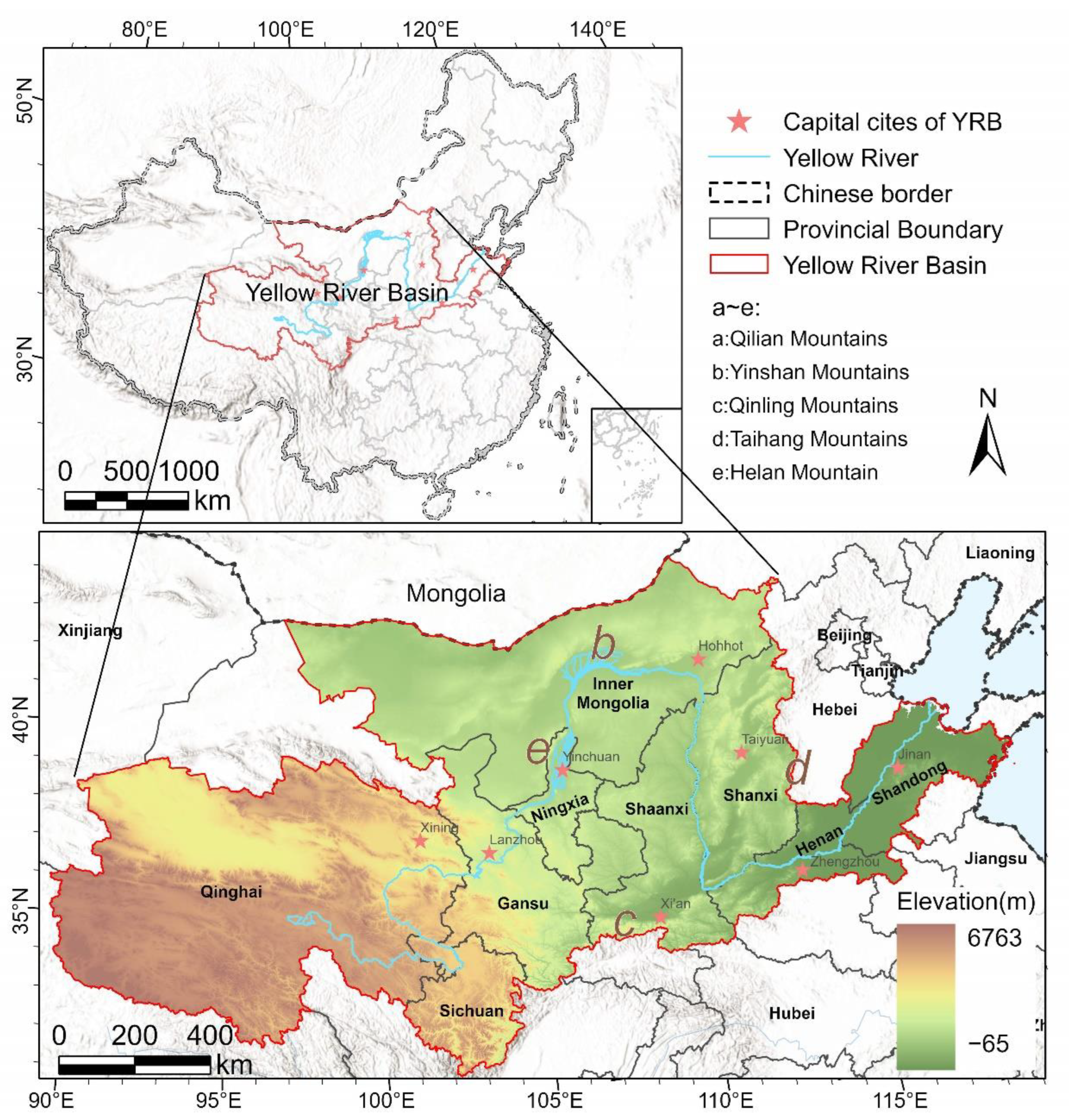
2.1. Study Area

The YRB is located in the transition zone of alpine, arid, semi-arid, and semi-humid areas in China, with a diverse climate, topography, and vegetation [26]. It flows through Qinghai, Sichuan, Gansu, Ningxia, Inner Mongolia, Shaanxi, Shanxi, Henan, and Shandong provinces, spanning the three major areas of east, middle, and west China, with a total length of about 5464 km and a watershed area of 795,000 km². There are ecologically fragile areas and important ecological function areas such as the Loess Plateau, Mu Us Sandy Land, and Kubuqi Desert. There are also important grain-producing areas and areas rich in resources and energy, such as the Fenwei Plains, Hetao Irrigation area, and Ningxia irrigation area. Based on the natural YRB and considering the integrity of administrative divisions and the direct relationship between regional economic development and the YRB, this paper defines the study area as nine provincial administrative divisions, with a total of 73 prefecture-level cities (Figure 1).

2.2. Data Processing

The LUCC data from 1985 to 2019 were from the China land-cover dataset (CLCD), with a spatial resolution of 30 m. It covers nine land-use types: crop, forest, shrub, grassland, water, snow and ice, barren, impervious surface, and wetlands [27]. The overall classification accuracy is 76.45% for larger land areas, such as crop, forest, and grassland, showing a better classification effect. It has better classification accuracy and wider time coverage than the existing land-cover products. Digital Elevation Model (DEM) data were from the Geospatial Data Cloud (http://www.gscloud.cn/search (accessed on 10 July 2022)) ASTER GDEM 30 m dataset with spatial resolution of 30 m. Soil erodibility data were calculated from the Harmonized World Soil Database (http://data.tpdc.ac.cn (accessed on 22 August 2022)) for soil texture, sand content, silt content, clay content, and soil organic-carbon content. Rainfall erosion data were from the European Commission (https://esdac.jrc.ec.europa.eu/content/global-rainfall-erosivity (accessed on 22 August 2022)), with a spatial resolution of 1 km. The spatial resolution of the ERS distribution map extracted from the CLCD dataset was 30 m. Because the computing grid of ESs contains different spatial resolutions from 30 m to 1 km, the resampling tool was used to unify the input grid into 1 km to analyze the spatial expression of ESs. The data were transformed into a unified projected coordinate system (Lambert Conformal Conic).

2.3. Methods

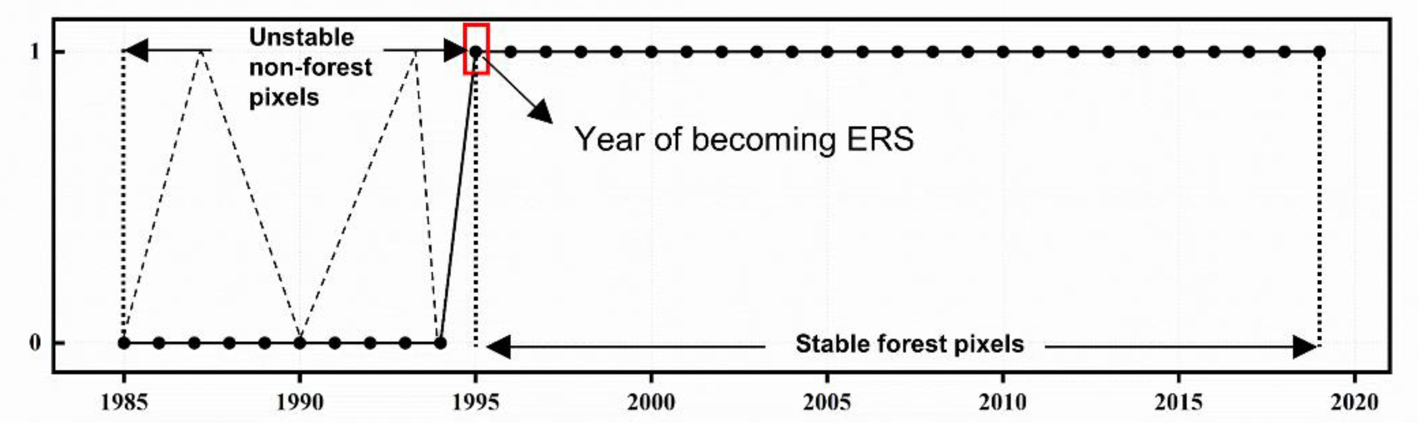
2.3.1. Trajectory Analysis to Map Ecological Restoration Space

Referring to the definition of ecological land by relevant scholars [28] and policy documents (http://www.gov.cn/zhengce/2017-02/07/content_5166291.htm (accessed on 22 August 2022)), this study defines ecological land as forest, grassland, and shrub. ERS spatial identification is defined by pixel-scale CLCD product land-use conversion, that is, the spatial expansion and quantity increase caused by the conversion of other land types to ecological land.

This study used to the temporal-segmentation and change-detection methods [29]. We propose a spatial recognition method of “Ecological restoration trajectories” based on the interannual ERS dynamic identification research targets. These research targets include two objectives: (1) Spatial distribution and physical location of ERS in the YRB; (2) Dynamic evolution characteristics of ERS in a long time sequence. In particular, given that when a pixel changes from cropland, barren land, and construction land to ecological land at a given time, it remains ecological land for the rest of the time, we call them “Ecological restoration trajectories”. Considering the time effect of land-type conversion and the long growth period of vegetation restoration, we detected LUCC time series at 5-year intervals. ERS was divided into three subcategories: forest restoration space (FRS), grassland restoration space (GRS), and shrub restoration space (SRS). Taking the identification of FRS as an example (Figure 2), the procedure includes these core steps: first, all the pixels in the land-cover sequence were set to 1, and all other land-cover classes were set to 0. If the pixel is a nonforest pixel (that is, a value of 0) that changes to a forest-cover type after five years and remains a forest-cover type in subsequent years, then the pixel has undergone forest restoration in a particular year; the exact year of forest restoration is defined as the first year in which the pixel becomes forest. Considering the importance of the contribution of different land covers to the ecosystem [30], when identifying SRS to eliminate forest pixels, we must identify GRS to eliminate forest and shrub pixels. When forest changed into shrub or grassland, seen as the natural-evolution-induced types referring to the gradual changes in the evolution process of the natural ecosystem or the indirect interference of human beings, such as the land degradation led by desertification and salinization [31], we do not consider ecological restoration to have occurred.

2.3.2. Ecosystem Services Assessment and Mapping

Three key ESs were selected for quantitative evaluation: (1) HQ; (2) CS; and (3) SC. The selection was based on the following criteria: (1) The availability of complete data and significant correlation with restoration practices in the study area; (2) Taking into account the focus of the study and the dynamics of the long time series of ESs, the ESs were selected from the supply modules of the three main ecosystem types (supply, regulation, and cultural services) described in the Millennium Ecosystem Assessment [32].

(1)

Habitat quality

We used the habitat-quality module in the InVEST model to calculate habitat quality in the YRB to quantify the biodiversity. The formula is as follows.

$$Q_{xj}=H_j\left[1-\left(\frac{D_{xj}^z}{D_{xj}^z+k^z}\right)\right]$$

(1)

where $Q_{xj}$ is the habitat quality of the $x$ grid in class $j$ land cover, ranging from 0 (unsuitable habitat) to 1 (optimum habitat); $H_j$ is the habitat suitability of class $j$ land cover; $D_{xj}$ is the threat level of grid $x$ in class $j$ land cover; $z$ is the scale parameter, default 2.5; $k$ is the semisaturation constant, initially set to 0.5. The $k$ value is usually set to half the maximum $D_{xj}$. We used the default $k$ value to run the program and found that the maximum $D_{xj}$ in the study area is 0.30, so we set the $k$ value to 0.15. The related factors are listed in Table S1.

(2)

Carbon storage

We used the carbon storage and sequestration module in the InVEST model to calculate carbon-storage content in the YRB. The formula is as follows:

$$C_{i }=C_{i-above }+C_{i-below }+C_{i-soil}+C_{i-dead }$$

(2)

$$\begin{array}{c}{C}_{total }={\displaystyle {\displaystyle \sum }_{i=1}^n}{C}_i\times S_i\end{array}$$

(3)

where i is the type i of land cover, $C_{\mathrm{i}}$ is the total carbon density of soil and organism, Mg hm⁻²; $C_{i-above }$ is the aboveground-part carbon density (from all plant materials above the soil), Mg hm⁻²; $C_{\mathrm{i}-below }$ is the underground-part carbon density, (from living plant root systems), Mg hm⁻²; $C_{\mathrm{i}-soil}$ is the soil-carbon density, (from organic and mineral soils), Mg hm⁻²; $C_{\mathrm{i}-dead }$ is the soil-carbon density for the density of dead organic carbon, (from litter or standing dead trees), Mg hm⁻²; $C_{total }$ is total carbon storage, Mg; $S_i$ the total area of the i land cover, hm⁻²; and $n$ is the number of land-cover types. The carbon density of each land cover can be seen in Table S2.

(3)

Soil Conservation

The calculation of soil conservation is based on the sediment-delivery-ratio module of the InVEST model, which is mainly derived from the soil-loss equation (USLE). The formula is as follows:

$$SC=Ap-Ar=R\times K\times LS\times \left(1-C\times P\right)$$

(4)

where SC is the soil-holding capacity (Mg hm⁻²), 𝐴𝑝 is potential soil erosion, and 𝐴𝑟 is actual soil erosion. R is rainfall erosivity derived from the published global dataset, MJ·mm·hm⁻²·h⁻¹·yr⁻¹. K is the soil-erodibility factor, which is calculated by the erosion-productivity-evaluation model (EPIC) proposed by Williams and Arnold [33]. LS is the slope-length factor. C is the vegetation-cover and -management factor; P is the factor of soil-conservation measures. In the model, P and C values are fixed values used to adjust the actual deviation of the calculated SC (Table S3).

2.3.3. Global-Spatial-Autocorrelation Analysis

The Moran’s I statistic has demonstrated its effectiveness in measuring the potential interdependence and heterogeneity of geographic data within the same distribution area [34]. We used global spatial autocorrelation to explore the spatial autocorrelation and aggregation of ERS in global space. Combining the size of the study area with the actual results, the study area was divided into 15 km × 15 km grids, which enabled us to mine LUCC information and detect spatial heterogeneity on a more microscale than a different administrative boundary. At the same time, it solved the natural conflict between the basic unit of the ecosystem and the boundary of the administrative division. The formula is as follows:

$$I=\frac{N{{\displaystyle \sum }}_i{{\displaystyle \sum }}_j{w}_{ij}\left(x_i-\overline{x}\right)\left(x_j-\overline{x}\right)}{\left({{\displaystyle \sum }}_i{{\displaystyle \sum }}_j{w}_{ij}\right){{\displaystyle \sum }}_i{\left(x_i-\overline{x}\right)}^2}$$

(5)

where $I$ is the Global Moran’s I, the range of values is [−1, 1], and $I$ > 0 is the positive spatial correlation of ERS in the global space. The closer the correlation is to 1, the more significant the correlation is. If $I$ = 0, there is no spatial correlation. $N$ is the number of grids. $w_{ij}$ is the spatial-weight matrix, $x_i$ is the total area of ERS in a grid, and $\overline{x}$ is the average of ERS in all grids.

2.3.4. Spatial-Response Characterization

The geographically weighted-regression (GWR) model, an improvement in the traditional linear-regression model, is used to calculate the response characteristics of different ESs to grid-scale ERS. It applies spatial-weight matrices to linear-regression models so that the relationships between variables vary with spatial location, playing an excellent role in exploring spatial nonstationarity [35]. The formula is as follows:

$$y_i={\beta }_0\left(u_i+v_i\right)+\sum {\beta }_j\left(u_i+v_i\right)x_{ij}+{\epsilon }_i$$

(6)

where $y_i$ is the ESs change in different years of the grid $i$; ($u_i,v_i$) is the geographical coordinates of grid $i$; $j$ is the number of independent variables; $i$ is the number of grids; ${\beta }_0\left(u_i+v_i\right)$ is the intercept of grid $i$; ${\beta }_j\left(u_i+v_i\right)$ is the spatial regression coefficient of grid $i$; $x_{ij}$ is the value of the variable $j$ on grid $i$; and ${\epsilon }_i$ is the random-error term.

A significant spatial correlation of independent variables is a prerequisite for applying the GWR model [36]. Bandwidth significantly impacts the accuracy of the GWR model, and inappropriate bandwidth results in data redundancy or overfitting [37]. In this study, the Akaike Information Criterion (AIC) method was used to determine the optimal bandwidth, which considers the degree-of-freedom differences in different models and can solve the problem quickly and easily [38].

3. Results

3.1. Spatiotemporal Pattern and Evolution of Ecological Restoration Space

From 1990 to 2015, the total area of ERS in the YRB was 184,197.05 km² (Table S4). GRS was the largest subcategory of restoration space, accounting for 73.14% of the total area of ERS, followed by FRS (26.08%) and SRS (0.78%). As shown in Figure 3, Inner Mongolia, Qinghai, and Shaanxi were the three provinces with the largest area of ERS, where restoration space reached 41,012.76 km², 32,329.98 km², and 28,430.48 km², respectively (Figure 4g). Henan and Shandong, located in the middle and lower reaches of the YRB, were the provinces with the least restoration space, accounting for 2869.04 km² and 1801.84 km², respectively, less than 10% of the largest provinces.

As shown in Figure 4a–f, we found significant differences in spatiotemporal distribution among subcategories from 1990 to 2015. The spatial pattern of FRS was clustered in the eastern region and remains basically unchanged in the time series. It is mainly distributed in the middle reaches of the YRB, including the Qilian Mountains, Qinling Mountains, and Lvliang Mountains throughout the western Shanxi province, and the Taihang Mountains, Funiu Mountains, and Loess Plateau in the northern Guanzhong Basin, which had the largest area distribution, at 7517.94 km² in 2015. The variation in GRS was severe, with the coefficient of variation in inter-annual distribution being 42.34%. In 1990, the area was only 2736.93 km², distributed locally in northern Gansu and Qinghai. It may be that the grassland restoration before 1990 was mainly spontaneous by individuals and did not rise to government behavior. The distribution area in 2015 was 31,449.88 km², which was directly related to the BTSSC launched in 2002. The Kubuqi Desert, the Mu Us Sandy Land of the Ordos Plateau, and the Loess Plateau had large GRS areas. This is evidence of China’s soil and water conservation in the Loess Plateau. SRS was mainly distributed in the Qilian Mountains and Qinling Mountains, but a small amount was distributed in the Lvliang Mountains and Taihang Mountains. The least distributing year was 1990, with 11.90 km². By 1995, the area had increased by 12.13 times, but only to 144.19 km². In the following 20 years, the area of SRS increased year by year and reached 447.73 km² in 2015. Evidently, the status of drought and water shortage in the Yellow River Basin is not suitable for shrub restoration.

Furthermore, the changing trend in all subcategories was reflected by the positioning of the spatial-distribution geographic center of each ERS subcategory in different years. The interannual variation in the geographic center of the ERS showed an obvious migration rule (Figure 4h). Affected by extensive ecological restoration in the northern Loess Plateau and Taihang Mountains, the geographic centers of FRS and GRS fluctuated from southwest to northeast. The migration trend in FRS is obvious, and the migration distance was 179.39 km. Due to the continuous expansion of SRS in the Qilian Mountains and Qinling Mountains in the southwestern YRB, the migration path of SRS showed the opposite rule compared with FRS and GRS. It generally moved southwest, and then northeast again twice.

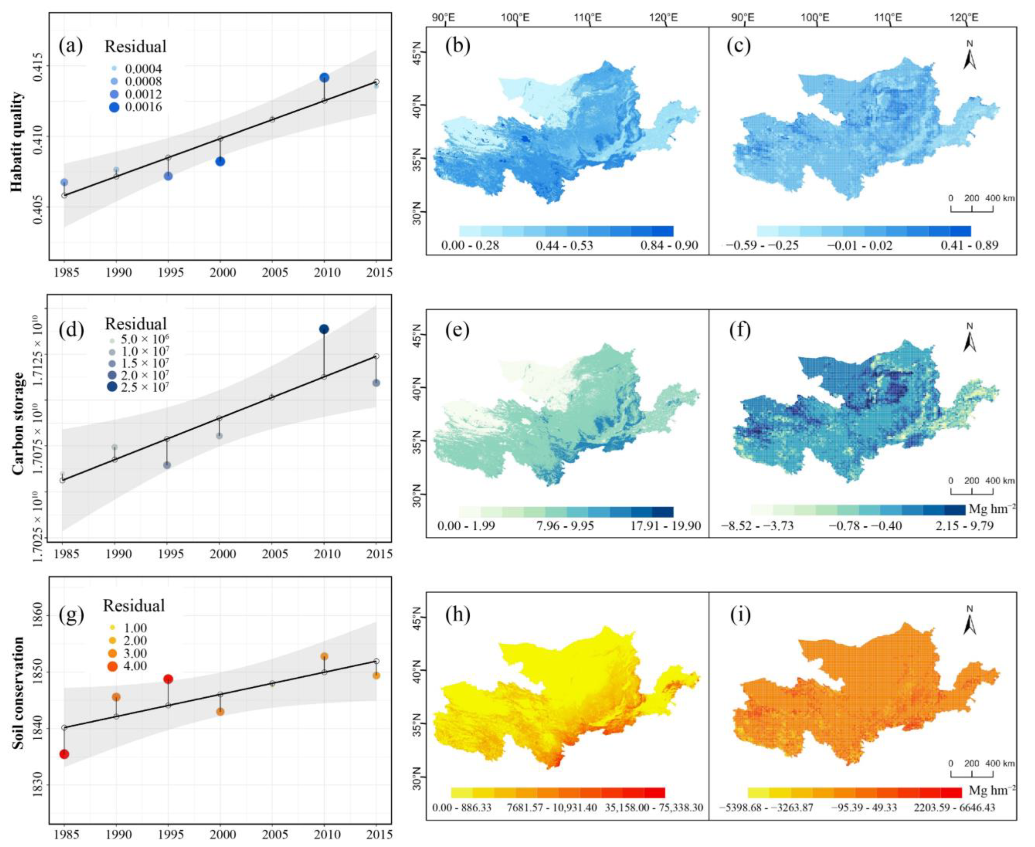
3.2. Spatial Variation Characteristics of Ecosystem Services

The YRB pixel-level ESs map for 2015 and the grid-scale dynamic-change map for 1990–2015 were generated (Figure 5). The three ESs’ distribution had a certain consistency and showed similar spatial patterns (low value in northwest and southeast areas, and high value in south and central areas) (Figure 5b,e,h). The high-value areas were concentrated in the Qinling Mountains, the eastern extension of the Taihang Mountains, and the Lvliang Mountains. The low-value areas were mainly located in the urban built-up areas, including Xi’an, Zhengzhou, Taiyuan, Qingdao, and other major cities in the YRB. In addition, there were large barren areas in the west of Inner Mongolia and northwest of Qinghai, which are the reasons for the low ESs value. From the perspective of heterogeneity, in Qinghai Lake, located in the northwestern Qinghai Province, the value of HQ was high, while the value of CS and SC were low. In the north of the YRB, the value of HQ and CS were medium, while the value of SC was low.

The dynamic changes in HQ, CS, and SC grid-scale from 1990 to 2015 are shown in Figure 5c,f,i. According to the results of spatial statistical analysis, the average HQ increased significantly since 1990, from 0.4076 in 1990 to 0.4135 in 2015, with an increase of 48.33% at grid-scale (Figure 5a,c). The total amount of CS increased dynamically (Figure 5d). In stages, 2010 was an important node year for total CS changes. From 1985 to 2010, the CS increased by 78.83 × 10⁶ Mg. After 2010, the YRB’s CS fell sharply, down 29.39 × 10⁶ Mg in 5 years, with an annual decline of 5.87 × 10⁶ Mg. The shrinking of grassland and the rapid expansion of construction land are the main reasons for the rapid decline of total CS. The average SC in 2015 was 1849.38 Mg hm⁻² (Figure 5g), while the highest SC was 75,538.30 Mg hm⁻². From 1990 to 2015, the area where SC significantly increased was 51.90% at grid-scale (Figure 5i).

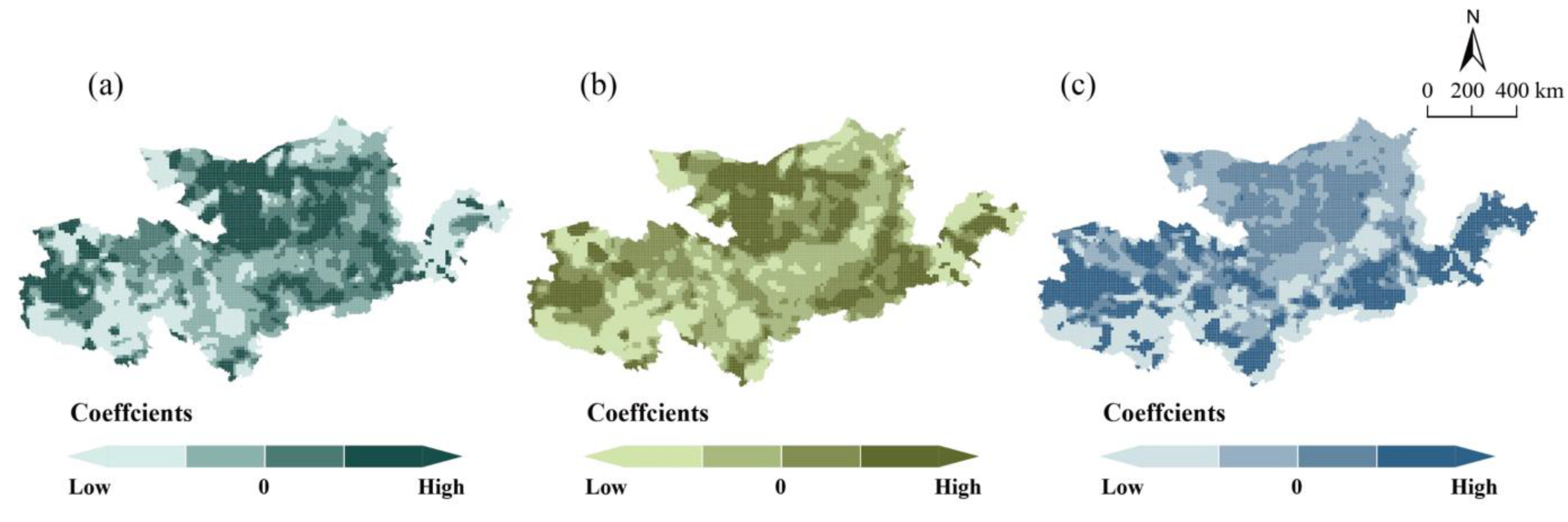
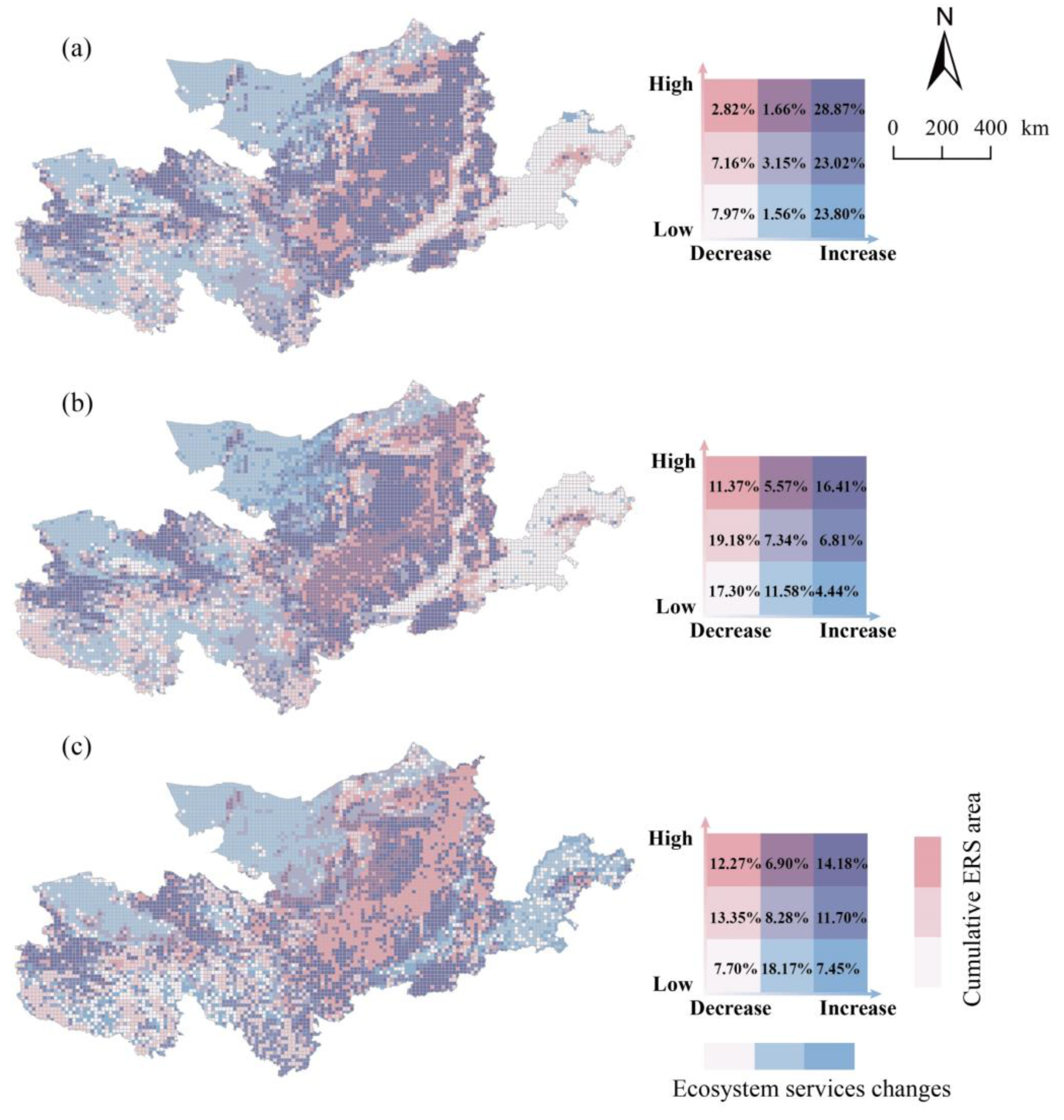
3.3. Spatial Response of Ecosystem Services on Ecological Restoration Space

The global Moran’s I was used to test the spatial aggregation relationship of ERS. The ERS Moran’s I from 1990 to 2015 is shown in Table S5. The ERS in the YRB showed significant aggregation characteristics in space in each year, and the standardized test Z values were greater than 2.58, which passed the significance test (p < 0.01).

There were significant spatial differences in the effects of ERS on ESs in different geographical grids (Figure 6). The distribution of ERS significantly improved the conditions of HQ, CS, and SC on 75.48%, 71.86%, and 56.75% of the grids, respectively. Among the three ESs, ERS had the most significant effect on SC. From 1990 to 2015, the maximum regression coefficients were all greater than 1. From 1990 to 1995, the maximum regression coefficient reached 45.74. Relatively, the effect of ERS on HQ is not obvious, although it had a wider positive influence scope (Table S6).

From the perspective of space, the spatial-response pattern of ESs on ERS has certain homogeneity. ERS had a significant effect on HQ and CS in western Qinghai, along the Yinshan Mountains in Inner Mongolia, northern Ningxia, and northwestern Henan. The regions where ERS had a significant promotion effect on SC showed obvious latitude characteristics, mainly distributed along both sides of 35° N, and a large number were concentrated in Qinghai, Shaanxi, Henan, Shandong, and other provinces. Sichuan, Shanxi, and other provinces also had extremely fragmented distribution. The contribution of subcategories of ERS to different ESs showed certain distribution rules. For example, the GRS widely distributed in Inner Mongolia, western Qinghai, Ningxia, and other places were spatially consistent with the distribution of the positive significant indigenous contribution of ERS to HQ. The FRS widely distributed in southern Gansu, Shanxi, Shaanxi, and northwestern Henan were consistent with the spatial distribution of ERS’ positive contribution to SC. In addition, we noted that when the area of ERS was too small, its contribution to ESs was mostly negatively correlated. In 1990–2015, in area where ERS had a negative effect on HQ, the average area of ERS was only 26.21% of the total average area of ERS. However, in area where ERS was large, the impact of ERS on ESs was not obvious or even weakly negatively correlated. The maximum regression coefficient of the grids with the first 20% of the ERS area to HQ was only 4 × 10⁻⁵, and 11.91% of the grids were less than or equal to 0. This indicates that the area of ERS in the grids had a threshold effect on ES. When the area of ERS in the grids was small or too large, the ecosystem resisted the ecological restoration behavior.

4. Discussion

4.1. Implications of the Obtained Results

Our research results showed that the spatial heterogeneity of ecological restoration intensity and type in different regions leads to different ecosystem changes, which, in turn, emphasizes the necessity of adopting different ecological-restoration intensities and types in ecosystem changes in different geographical units. By binary superposition of the cumulative area of ERS with the change values of ESs from 1990 to 2015, we divided the YRB for ecological restoration and green development into several situations (Figure 7).

(1)

Ecological restoration significantly improves ecosystem services. This type of area is the most powerful evidence of the positive impact of ecological restoration on ESs, and is more concentrated in the Loess Plateau. Considerable research has shown that the quality of the ecological environment in the Loess Plateau improved significantly due to ecological restoration [39,40,41].

(2)

Unobvious changes in ecosystem services accompany ecological restoration. Unfortunately, although large-scale ecological restoration had been carried out, the improvement trend in the environment in some regions was not apparent; in some cases, ecological degradation still occurred. We believe that although ecological restoration delays or hinders the trend in ecological degradation in ecologically fragile areas to some extent, its spatial quantity or time-series length is insufficient to reach the threshold of reversing degradation, that is, the lag effect of ERS on ESs. Although site-specific ecological-restoration activities, such as afforestation and grain for green, are being continuously implemented, it will be difficult and require a significant amount time to transform the structure of land properties and ecological functions due to the fragile nature of the region’s ecosystem. Intraspecific trade-offs in ESs may also be an important cause of this phenomenon [42]. Afforestation effectively reduces soil erosion and significantly enhances ESs such as SC and HQ, but deeper root systems of forest can utilize water stored in deeper soils under drought conditions [31], which significantly reduces water purification and causes trade-offs among ecosystem services in the region. In addition, the negative impacts of human activities such as overgrazing and reclamation also offset the positive effects of ecological restoration to a certain extent [20].

(3)

Obvious improvement in ecosystem services without ecological restoration. It should be noted where no ecological restoration activities were detected, but ESs tended to improve. The ecosystem quality in western Inner Mongolia and northwestern Qinghai improved significantly, but the cumulative area of ERS was tiny. From the perspective of time scale, ERS in western Inner Mongolia may have experienced a cycle of “degradation-restoration-redegradation” [43]. From a socioeconomic perspective, measures such as logging and grazing restrictions may lack necessary compensation for farmers and herdsmen, or the compensation amount provided may fall short of expectations. This has led to a negative impact on these projects, as some farmers and forestry workers have been dissuaded from participating in them, ultimately resulting in unsustainable ecological restoration activities [44]. From the natural perspective, the unsuccessful recruitment of dominant tree species in forests can trigger a process of vegetation succession, leading to the replacement of trees by understory species, and potentially even leading to desertification. Statistics showed that the survival rate of afforestation in arid and semi-arid regions of northern China since 1949 is only 15% [44], and the restoration of this unsustainable cycle was not recognized by our identification model. On the other hand, the weak basic foundation of ESs in the region had been greatly improved in phased and fragmented restoration activities, but the overall quality was still poor.

(4)

Ecosystem services continued to deteriorate without ecological restoration. This was roughly distributed in major urban agglomerations such as the Fenwei Plains and the middle and lower reaches of the YRB. With the continuous expansion of the urban built-up area, taking some provincial capitals in the middle and lower reaches of the YRB as examples, the construction land area of Zhengzhou City and Jinan City increased by 1179.90 km² and 881.30 km², respectively, from 1990 to 2019, and the land-use structure changed dramatically (Table S7), which led to the inevitable degradation and fragmentation of ecological land and damaged the complete material information flow process of the ecosystem. In addition, southern Inner Mongolia and the northern Loess Plateau also had some distribution. This part of the region belongs to ecologically fragile areas, which can lead to continued deterioration in the ecological environment when the value of ESs is insufficient to maintain the self-circulation of the system [45].

4.2. Suggestions for Ecological Restoration in the Yellow River Basin

We found that the spatial distribution of ERS in the YRB and its spatial response characteristics to ESs showed significant spatial heterogeneity, which was also verified in other existing studies [46,47]. The uneven spatial distribution of ERS and the spatial difference in the intensity of the ERS response to ESs can lead us to propose specific environmental-management strategies and green-development concepts for regional situations, and the one-size-fits-all management should not apply to all regions [48].

In the upper reaches of the YRB, the primary ecological restoration direction is the management of barren land and the implementation of desertification control. It is noteworthy that vast expanses of sandy land are distributed in the west of Inner Mongolia and northwest of Qinghai Province. While these two provinces have the largest cumulative ERS distribution areas among all provinces, the ERS cumulative areas account for less than 5% of the total administrative area of the provinces. Additionally, afforestation areas or grazing prohibition areas must be supplemented with appropriate ecological restoration measures to enhance the sustainability of ecological restoration, such as selecting tree species suitable for the local ecological environment and avoiding excessive grazing and other forms of human intervention.

In the middle and lower reaches of the YRB, the implementation of ecological restoration in urban built-up areas has high costs and little effect, and the rapid expansion of urban built-up areas is bound to occupy the niche of ERS, which is also consistent with our conclusion. With relatively high GDP, Henan and Shandong are the two provinces with the lowest cumulative area of ERS in the nine provinces. Despite the continuous expansion of urban built-up areas, the development of urban forests, such as urban parks, street trees, and green infrastructure can still effectively increase the supply of regional ecosystem services and urban resilience as ecological restoration measures within urban agglomerations [49]. How to find the Nash equilibrium point of ERS and other economic development occupation spaces will be an important proposition for green development and environmental management in the middle and lower reaches of the YRB.

4.3. Limitations and Future Work

Although some valuable results have been achieved, there are also some limitations. For example, ecological restoration includes natural recovery and anthropogenic intervention [50,51,52], while the ecological-restoration-trajectory model does not effectively divide the boundaries between natural recovery and anthropogenic intervention to define the contribution degrees of the two aspects. Vegetation changing from abandoned to fully regenerated can be detected by satellite with a period of delay [53]. This delay may cause misjudgment of ERS extraction and affect the accuracy of the extraction. In addition, the ecological restoration is a systematic project that involves human participation in decision-making and implementation. It is a multilevel structure practice coupled with nature, society, and ecology [54]. Therefore, further research is needed to understand how to better integrate socioeconomic factors into the optimization results.

5. Conclusions

The accurate identification of ERS and spatiotemporal pattern contributes to a more effective understanding the dramatic ecological-restoration practices occurring in the YRB. In this study, the ecological-restoration-trajectories model based on the CLCD dataset was integrated to analyze the spatiotemporal pattern and evolution of ERS. Supported by the ESs maps and the distribution of ERS, the GWR model was used to precisely measure the spatial relationship between ERS and ESs. The main contribution of this work can be summarized as follows:

(1)

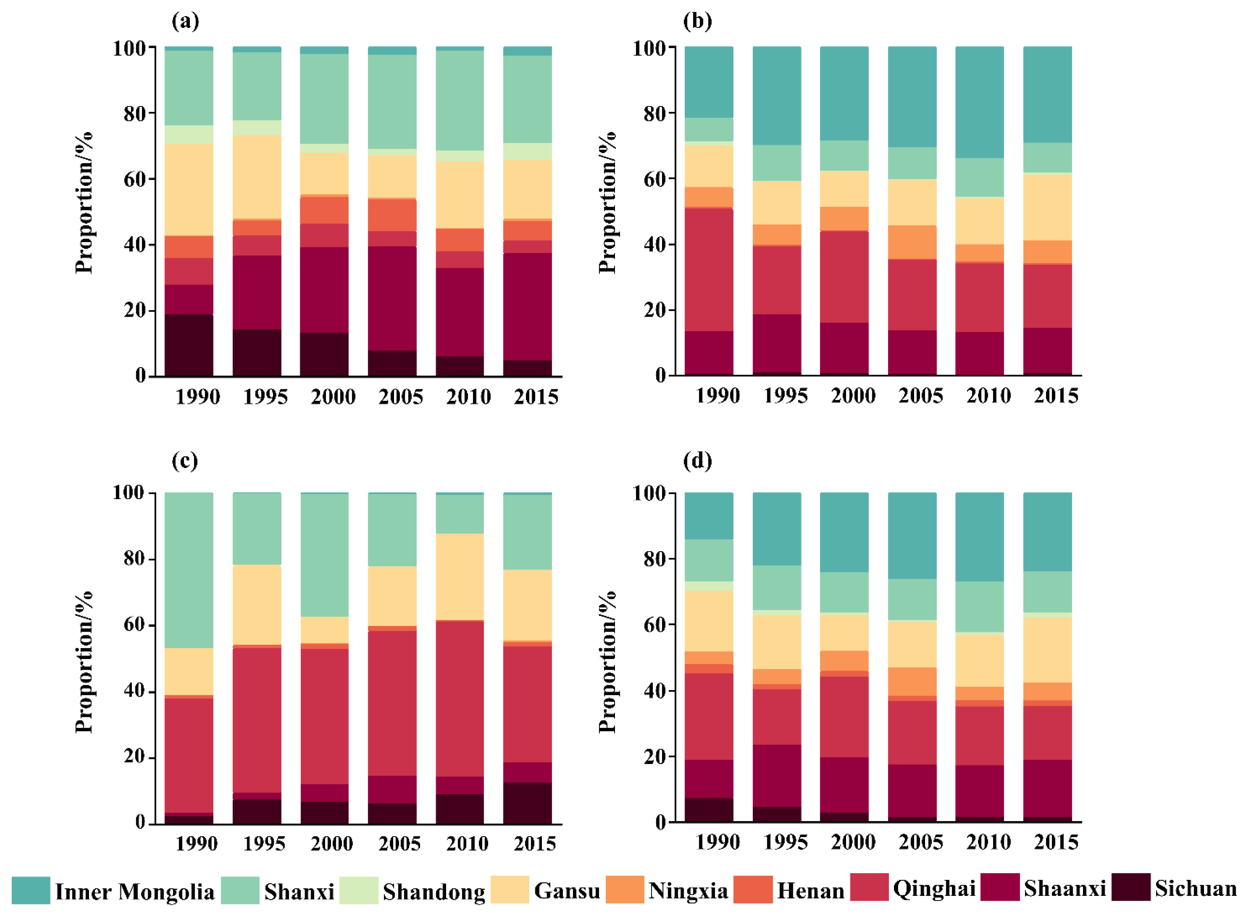
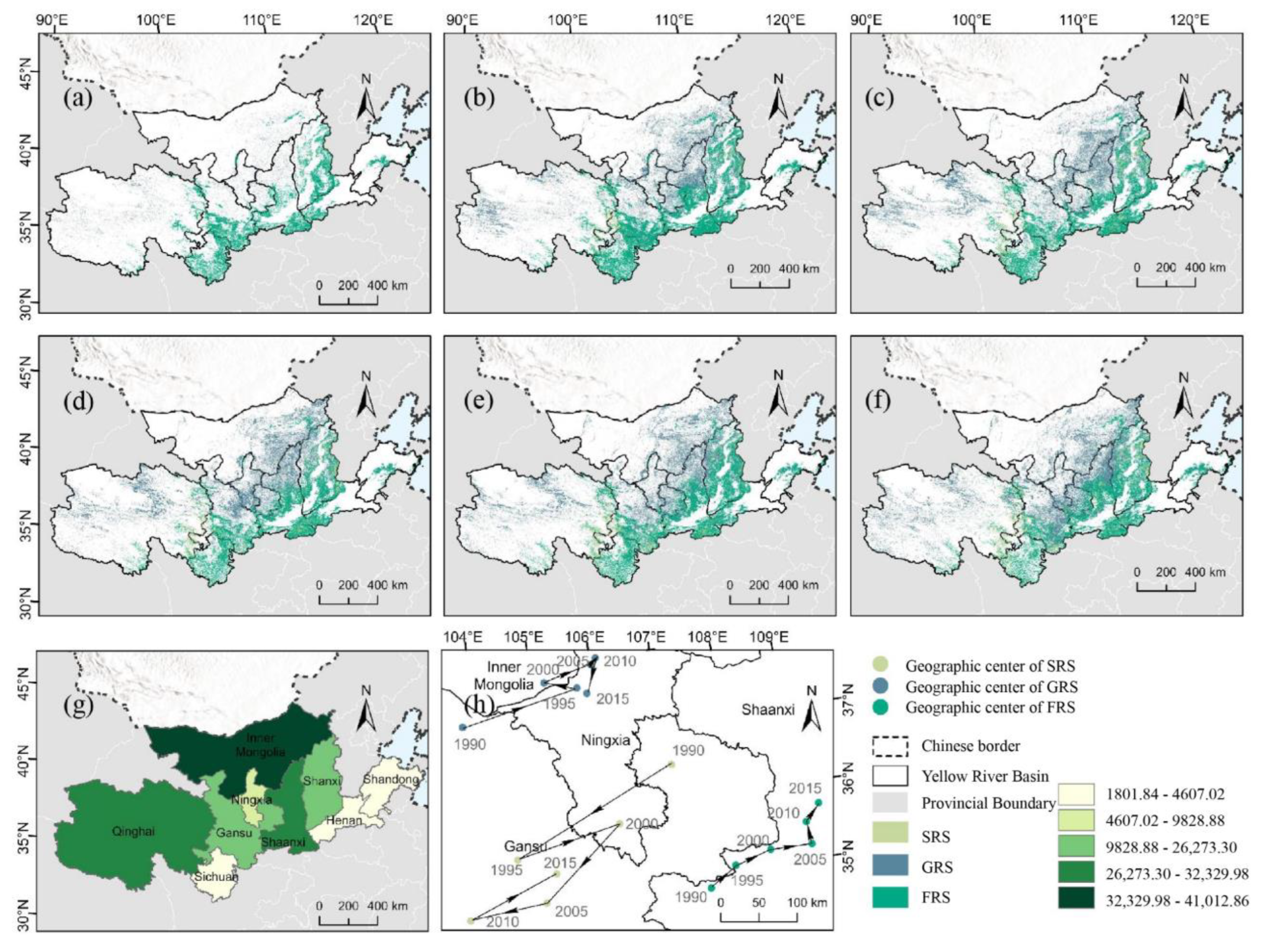
During 1990–2015, the spatial distribution of ERS continued to expand. By 2015, the cumulative area of ERS reached 184,197.05 km². Of the three ERS subcategories, GRS accounted for the largest area (73.14%), followed by FRS (26.08%) and SRS (0.78%). Afforestation was widely implemented in the Loess Plateau region, especially in Inner Mongolia, Qinghai, and Shaanxi provinces. The geographic centers of FRS, GRS, and SRS occurred in differential migration patterns, as FRS and GRS fluctuated from southwest to northeast, but the migration of SRS generally moved southwest.

(2)

The spatiotemporal heterogeneity of the three ESs at the regional and grid scales showed that HQ, CS, and SC experienced a significant increase during the past 30 years, but they all showed a downward trend in 2010. ERS modifies the land-use structure and information flow pattern of the ecosystem in the YRB, which has a significant effect on the different ecosystem services.

(3)

Our findings demonstrated that the distribution of ERS significantly improved the conditions of HQ, CS, and SC on 75.48%, 71.86%, and 56.75% of land across the YRB, respectively. Regional differentiation distribution of ERS can improve integrated ecosystem quality.

This study provided management experiences for meticulous ecological-restoration-zoning management and promoted sustainable land development in the YRB and other ecologically vulnerable areas with analogous ecological problems.

References

1. Millennium Ecosystem Assessment (Program) (Ed.) Ecosystems and Human Well-Being: Synthesis; Island Press: Washington, DC, USA, 2005; ISBN 978-1-59726-040-4. [Google Scholar]
2. Sabine, B.R.; Mathieu, G.; Olivier, B.; Miska, L.; Carmen, C.; Gregoire, M.; Antoine, G. From White to Green: Snow Cover Loss and Increased Vegetation Productivity in the European Alps. Science 2022, 376, 1119–1122. [Google Scholar]
3. Semenchuk, P.; Plutzar, C.; Kastner, T.; Matej, S.; Bidoglio, G.; Erb, K.-H.; Essl, F.; Haberl, H.; Wessely, J.; Krausmann, F.; et al. Relative Effects of Land Conversion and Land-Use Intensity on Terrestrial Vertebrate Diversity. Nat. Commun. 2022, 13, 615. [Google Scholar] [CrossRef] [PubMed]
4. Xie, H.; Zhang, Y.; Wu, Z.; Lv, T. A Bibliometric Analysis on Land Degradation: Current Status, Development, and Future Directions. Land 2020, 9, 28. [Google Scholar] [CrossRef] [Green Version]
5. United Nations. United Nations Decade on Ecosystem Restoration (2021–2030); United Nations: New York, NY, USA, 2019; Volume 19-03519, pp. 1–6. Available online: https://documents-dds-ny.un.org/doc/UNDOC/GEN/N19/060/16/PDF/N1906016.pdf?OpenElement. (accessed on 1 July 2022).
6. Chen, C.; Park, T.; Wang, X.; Piao, S.; Xu, B.; Chaturvedi, R.K.; Fuchs, R.; Brovkin, V.; Ciais, P.; Fensholt, R.; et al. China and India Lead in Greening of the World through Land-Use Management. Nat. Sustain. 2019, 2, 122–129. [Google Scholar] [CrossRef] [PubMed]
7. Hu, J.; Zhou, Q.; Cao, Q.; Hu, J. Effects of Ecological Restoration Measures on Vegetation and Soil Properties in Semi-Humid Sandy Land on the Southeast Qinghai-Tibetan Plateau, China. Glob. Ecol. Conserv. 2022, 33, e02000. [Google Scholar] [CrossRef]
8. Huang, C.; Zhou, Z.; Peng, C.; Teng, M.; Wang, P. How Is Biodiversity Changing in Response to Ecological Restoration in Terrestrial Ecosystems? A Meta-Analysis in China. Sci. Total Environ. 2019, 650, 1–9. [Google Scholar] [CrossRef] [PubMed]
9. Bastin, J.-F.; Finegold, Y.; Garcia, C.; Mollicone, D.; Rezende, M.; Routh, D.; Zohner, C.M.; Crowther, T.W. The Global Tree Restoration Potential. Science 2019, 364, 76–79. [Google Scholar] [CrossRef]
10. Temperton, V.M.; Buchmann, N.; Buisson, E.; Durigan, G.; Kazmierczak, Ł.; Perring, M.P.; de Sá Dechoum, M.; Veldman, J.W.; Overbeck, G.E. Step Back from the Forest and Step up to the Bonn Challenge: How a Broad Ecological Perspective Can Promote Successful Landscape Restoration. Restor. Ecol. 2019, 27, 705–719. [Google Scholar] [CrossRef] [Green Version]
11. Cao, S.; Chen, L.; Shankman, D.; Wang, C.; Wang, X.; Zhang, H. Excessive Reliance on Afforestation in China’s Arid and Semi-Arid Regions: Lessons in Ecological Restoration. Earth Sci. Rev. 2011, 104, 240–245. [Google Scholar] [CrossRef]
12. Lyu, R.; Clarke, K.C.; Zhang, J.; Feng, J.; Jia, X.; Li, J. Dynamics of Spatial Relationships among Ecosystem Services and Their Determinants: Implications for Land Use System Reform in Northwestern China. Land Use Policy 2021, 102, 105231. [Google Scholar] [CrossRef]
13. Wheeler, B.W.; Lovell, R.; Higgins, S.L.; White, M.P.; Alcock, I.; Osborne, N.J.; Husk, K.; Sabel, C.E.; Depledge, M.H. Beyond Greenspace: An Ecological Study of Population General Health and Indicators of Natural Environment Type and Quality. Int. J. Health Geogr. 2015, 14, 17. [Google Scholar] [CrossRef] [PubMed] [Green Version]
14. Lian, J.J.; Chen, H.S.; Wang, F.; Nie, Y.P.; Wang, K.L. Separating the Relative Contributions of Climate Change and Ecological Restoration to Runoff Change in a Mesoscale Karst Basin. Catena 2020, 194, 104705. [Google Scholar] [CrossRef]
15. Yang, H.F.; Mu, S.J.; Li, J.L. Effects of Ecological Restoration Projects on Land Use and Land Cover Change and Its Influences on Territorial NPP in Xinjiang, China. Catena 2014, 115, 85–95. [Google Scholar] [CrossRef]
16. Ding, Z.; Liu, Y.; Wang, L.C.; Chen, Y.A.; Yu, P.J.; Ma, M.G.; Tang, X.G. Effects and Implications of Ecological Restoration Projects on Ecosystem Water Use Efficiency in the Karst Region of Southwest China. Ecol. Eng. 2021, 170, 106356. [Google Scholar] [CrossRef]
17. Yang, G.; Li, Y.; Huang, T.Q.; Fu, B.L.; Tang, J.; Zhang, X.; Wu, J.S. Multi-Scale Evaluation of Ecological Restoration Effects in the Riparian Zone Using Landsat Series Images from 1980 to 2019. Ecol. Indic. 2021, 132, 108342. [Google Scholar] [CrossRef]
18. Zhai, T.; Huang, L. Linking MSPA and Circuit Theory to Identify the Spatial Range of Ecological Networks and Its Priority Areas for Conservation and Restoration in Urban Agglomeration. Front. Ecol. Evol. 2022, 10, 1–16. [Google Scholar] [CrossRef]
19. Costanza, R.; d’Arge, R.; de Groot, R.; Farber, S.; Grasso, M.; Hannon, B.; Limburg, K.; Naeem, S.; O’Neill, R.V.; Paruelo, J.; et al. The Value of the World’s Ecosystem Services and Natural Capital. Nature 1997, 387, 253–260. [Google Scholar] [CrossRef]
20. Jiang, C.; Wang, F.; Zhang, H.; Dong, X. Quantifying Changes in Multiple Ecosystem Services during 2000–2012 on the Loess Plateau, China, as a Result of Climate Variability and Ecological Restoration. Ecol. Eng. 2016, 97, 258–271. [Google Scholar] [CrossRef]
21. Wang, Y.; Li, B. Dynamics Arising from the Impact of Large-scale Afforestation on Ecosystem Services. Land Degrad. Dev. 2022, 33, 3186–3198. [Google Scholar] [CrossRef]
22. Wen, X.; Théau, J. Spatiotemporal Analysis of Water-Related Ecosystem Services under Ecological Restoration Scenarios: A Case Study in Northern Shaanxi, China. Sci. Total Environ. 2020, 720, 137477. [Google Scholar] [CrossRef]
23. Chen, X.; Yu, L.; Du, Z.; Xu, Y.; Zhao, J.; Zhao, H.; Zhang, G.; Peng, D.; Gong, P. Distribution of Ecological Restoration Projects Associated with Land Use and Land Cover Change in China and Their Ecological Impacts. Sci. Total Environ. 2022, 825, 153938. [Google Scholar] [CrossRef]
24. Li, Q.; Shi, X.Y.; Wu, Q.Q. Effects of Protection and Restoration on Reducing Ecological Vulnerability. Sci. Total Environ. 2021, 761, 143180. [Google Scholar] [CrossRef]
25. Lu, F.; Hu, H.F.; Sun, W.J.; Zhu, J.J.; Liu, G.B.; Zhou, W.M.; Zhang, Q.F.; Shi, P.L.; Liu, X.P.; Wu, X.; et al. Effects of National Ecological Restoration Projects on Carbon Sequestration in China from 2001 to 2010. Proc. Natl. Acad. Sci. USA 2018, 115, 4039–4044. [Google Scholar] [CrossRef] [PubMed] [Green Version]
26. Jiang, W.G.; Yuan, L.H.; Wang, W.J.; Cao, R.; Zhang, Y.F.; Shen, W.M. Spatio-Temporal Analysis of Vegetation Variation in the Yellow River Basin. Ecol. Indic. 2015, 51, 117–126. [Google Scholar] [CrossRef]
27. Yang, J.; Huang, X. The 30 m Annual Land Cover Dataset and Its Dynamics in China from 1990 to 2019. Earth Syst. Sci. Data 2021, 13, 3907–3925. [Google Scholar] [CrossRef]
28. Peng, J.; Zhao, M.; Guo, X.; Pan, Y.; Liu, Y. Spatial-Temporal Dynamics and Associated Driving Forces of Urban Ecological Land: A Case Study in Shenzhen City, China. Habitat Int. 2017, 60, 81–90. [Google Scholar] [CrossRef]
29. Du, Z.R.; Yang, J.Y.; Ou, C.; Zhang, T.T. Agricultural Land Abandonment and Retirement Mapping in the Northern China Crop-Pasture Band Using Temporal Consistency Check and Trajectory-Based Change Detection Approach. IEEE Trans. Geosci. Remote Sens. 2022, 60, 1–12. [Google Scholar] [CrossRef]
30. Song, X.P. Global Estimates of Ecosystem Service Value and Change: Taking Into Account Uncertainties in Satellite-Based Land Cover Data. Ecol. Econ. 2018, 143, 227–235. [Google Scholar] [CrossRef]
31. Chang, X.; Xing, Y.; Wang, J.; Yang, H.; Gong, W. Effects of Land Use and Cover Change (LUCC) on Terrestrial Carbon Stocks in China between 2000 and 2018. Resour. Conserv. Recycl. 2022, 182, 106333. [Google Scholar] [CrossRef]
32. Zhang, Y.; Liu, Y.; Zhang, Y.; Liu, Y.; Zhang, G.; Chen, Y. On the Spatial Relationship between Ecosystem Services and Urbanization: A Case Study in Wuhan, China. Sci. Total Environ. 2018, 637–638, 780–790. [Google Scholar] [CrossRef]
33. Williams, J.R.; Arnold, J.G. A System of Erosion-Sediment Yield Models. Soil Technol. 1997, 11, 43–55. [Google Scholar] [CrossRef]
34. Liu, Q.; Wu, Y.; Zhou, Y.; Li, X.; Yang, S.; Chen, Y.; Qu, Y.; Ma, J. A Novel Method to Analyze the Spatial Distribution and Potential Sources of Pollutant Combinations in the Soil of Beijing Urban Parks. Environ. Pollut. 2021, 284, 117191. [Google Scholar] [CrossRef] [PubMed]
35. Liu, C.; Wu, X.; Wang, L. Analysis on Land Ecological Security Change and Affect Factors Using RS and GWR in the Danjiangkou Reservoir Area, China. Appl. Geogr. 2019, 105, 1–14. [Google Scholar] [CrossRef]
36. Wu, R.; Zhang, J.; Bao, Y.; Tong, S. Using a Geographically Weighted Regression Model to Explore the Influencing Factors of CO2 Emissions from Energy Consumption in the Industrial Sector. Pol. J. Environ. Stud. 2016, 25, 2641–2652. [Google Scholar] [CrossRef]
37. Wang, S.; Liu, Z.; Chen, Y.; Fang, C. Factors Influencing Ecosystem Services in the Pearl River Delta, China: Spatiotemporal Differentiation and Varying Importance. Resour. Conserv. Recycl. 2021, 168, 105477. [Google Scholar] [CrossRef]
38. Pineda Jaimes, N.B.; Bosque Sendra, J.; Gómez Delgado, M.; Franco Plata, R. Exploring the Driving Forces behind Deforestation in the State of Mexico (Mexico) Using Geographically Weighted Regression. Appl. Geogr. 2010, 30, 576–591. [Google Scholar] [CrossRef]
39. Dang, X.; Liu, G. Emergy Measures of Carrying Capacity and Sustainability of a Target Region for an Ecological Restoration Programme: A Case Study in Loess Hilly Region, China. J. Environ. Manag. 2012, 102, 55–64. [Google Scholar] [CrossRef]
40. He, J.; Shi, X.; Fu, Y. Identifying Vegetation Restoration Effectiveness and Driving Factors on Different Micro-Topographic Types of Hilly Loess Plateau: From the Perspective of Ecological Resilience. J. Environ. Manag. 2021, 289, 112562. [Google Scholar] [CrossRef]
41. Lü, Y.; Fu, B.; Feng, X.; Zeng, Y.; Liu, Y.; Chang, R.; Sun, G.; Wu, B. A Policy-Driven Large Scale Ecological Restoration: Quantifying Ecosystem Services Changes in the Loess Plateau of China. PLoS ONE 2012, 7, e31782. [Google Scholar] [CrossRef] [Green Version]
42. Feng, Q.; Zhao, W.; Hu, X.; Liu, Y.; Daryanto, S.; Cherubini, F. Trading-off Ecosystem Services for Better Ecological Restoration: A Case Study in the Loess Plateau of China. J. Clean. Prod. 2020, 257, 120469. [Google Scholar] [CrossRef]
43. Feng, R.; Wang, F.; Wang, K. Spatial-Temporal Patterns and Influencing Factors of Ecological Land Degradation-Restoration in Guangdong-Hong Kong-Macao Greater Bay Area. Sci. Total Environ. 2021, 794, 148671. [Google Scholar] [CrossRef]
44. Cao, S. Why Large-Scale Afforestation Efforts in China Have Failed To Solve the Desertification Problem. Environ. Sci. Technol. 2008, 42, 1826–1831. [Google Scholar] [CrossRef] [PubMed] [Green Version]
45. Wang, X.; Ma, X.; Feng, X.; Zhou, C.; Fu, B. Spatial-Temporal Characteristics of Trade-off and Synergy of Ecosystem Services in Key Vulnerable Ecological Areas in China. Shengtai Xuebao 2019, 39, 7344–7355. [Google Scholar] [CrossRef]
46. Wang, Y.; Wang, H.; Liu, G.; Zhang, J.; Fang, Z. Factors Driving Water Yield Ecosystem Services in the Yellow River Economic Belt, China: Spatial Heterogeneity and Spatial Spillover Perspectives. J. Environ. Manag. 2022, 317, 115477. [Google Scholar] [CrossRef]
47. Yang, J.; Xie, B.; Zhang, D.; Tao, W. Climate and Land Use Change Impacts on Water Yield Ecosystem Service in the Yellow River Basin, China. Environ. Earth Sci. 2021, 80, 1–12. [Google Scholar] [CrossRef]
48. Liu, Y.; Li, J.; Yang, Y. Strategic Adjustment of Land Use Policy under the Economic Transformation. Land Use Policy 2018, 74, 5–14. [Google Scholar] [CrossRef]
49. Bonilla-Bedoya, S.; Mora, A.; Vaca, A.; Estrella, A.; Herrera, M.Á. Modelling the Relationship between Urban Expansion Processes and Urban Forest Characteristics: An Application to the Metropolitan District of Quito. Comput. Environ. Urban Syst. 2020, 79, 101420. [Google Scholar] [CrossRef]
50. Crossman, N.D.; Bernard, F.; Egoh, B.; Kalaba, F.; Lee, N.; Moolenaar, S. The Role of Ecological Restoration and Rehabilitation in Production Landscapes: An Enhanced Approach to Sustainable Development. In Working Paper for the UNCCD Global Land Outlook; United Nations: New York, NY, USA, 2017. [Google Scholar]
51. Hu, Z.; Long, J.; Wang, X. Self-Healing, Natural Restoration and Artificail Restoration of Ecoligical Environment Foe Coal Mining. J. China Coal Soc. 2014, 59, 1751–1757. (In Chinese) [Google Scholar]
52. Li, X.S.; Wang, H.Y.; Zhou, S.F.; Sun, B.; Gao, Z.H. Did Ecological Engineering Projects Have a Significant Effect on Large-Scale Vegetation Restoration in Beijing-Tianjin Sand Source Region, China? A Remote Sensing Approach. Chin. Geogr. Sci. 2016, 26, 216–228. [Google Scholar] [CrossRef] [Green Version]
53. Crawford, C.; Yin, H.; Radeloff, V.; Wilcove, D. Rural Land Abandonment Is Too Ephemeral to Provide Major Benefits for Biodiversity and Climate. Sci. Adv. 2022, 8, eabm8999. [Google Scholar]
54. Cao, S.; Zheng, X.; Chen, L.; Ma, H.; Xia, J. Using the Green Purchase Method to Help Farmers Escape the Poverty Trap in Semiarid China. Agron. Sustain. Dev. 2017, 37, 7. [Google Scholar] [CrossRef] [Green Version]
Figure 1. Location and topography of the YRB, China.
Land 12 00730 g001
Figure 2. The schematic diagram of ERS dynamic identification method.
Land 12 00730 g002
Figure 3. The temporal variation in (d) ERS and three subcategories((a) FRS, (b) GRS, (c) SRS) in different provinces of the YRB.
Land 12 00730 g003
Figure 4. Spatiotemporal pattern and evolution of ERS. (af) spatial distribution pattern of ERS in 1990, 1995, 2000, 2005, 2010, and 2015, respectively; (g) the cumulative area of ERS by province for 1990 to 2015, km2; (h) distribution of interannual migration pattern of geographic center of GRS, FRS, and SRS from 1990 to 2015.
Land 12 00730 g004
Figure 5. Spatial patterns and trends in ESs changes in YRB from 1985 to 2015 in (a) average habitat quality (d) total carbon storage, Mg (g) average soil conservation, Mg hm−2; Black line is the fitting curve of ESs interannual variation, point represents the regional observed values and predicted values for the year with 95% CI in gray. Residual is the absolute value of predicted values minus observed values; (b,e,h) pixel-scale habitat quality, carbon storage, and soil-conservation-distribution maps in 2015, respectively; (c,f,i) change trends in average habitat quality, carbon storage, and soil conservation by grid from 1990 to 2015, respectively.
Land 12 00730 g005
Figure 6. Spatial-response characteristics of different ESs to ERS from 1990 to 2015. (a) habitat quality; (b) carbon storage; (c) soil conservation. Regression coefficients greater than 0 represent a positive correlation between the cumulative area of ERS in different grids and the variation value of ESs. The darker the color, the higher the degree of influence of ERS on ESs.
Land 12 00730 g006
Figure 7. Overlaying the cumulative area of ERS on the changing values of ESs ((a) habitat quality; (b) carbon storage; (c) soil conservation) from 1990 to 2015. The color red indicates the cumulative area of ERS, with darker shades representing larger accumulated areas within each grid. The color blue denotes the changing value of ESs from 1990 to 2015, with darker shades indicating more pronounced changes. The percentage in the legend is the proportion of the number of grids in the corresponding interval.
Land 12 00730 g007
Disclaimer/Publisher’s Note: The statements, opinions and data contained in all publications are solely those of the individual author(s) and contributor(s) and not of MDPI and/or the editor(s). MDPI and/or the editor(s) disclaim responsibility for any injury to people or property resulting from any ideas, methods, instructions or products referred to in the content.