Zonation of a Viticultural Territorial Context in Piemonte (NW Italy) to Support Terroir Identification: The Role of Pedological, Topographical and Climatic Factors

Abstract

Grapevine production and quality greatly depend on site-specific features such as topography, soil, and climate. The possibility of recognizing and mapping local specificities of a wine-production area is highly desirable, as environmental conditions are the main drivers of wine production in terms of both quality and quantity. Areas showing similar features able to determine specific traits in vine and wine production are referred to as terroirs. It is commonly considered that soil and climate represent the main elements for a functional and balanced viticultural ecosystem; if they change, grapevine quality and yield change too, and this occurs in spite of any agronomic practice. Terroir mapping based on traditional methodology requires a considerable investment of time and money by producers and wine consortia; moreover, it preserves an important subjective component. In this work, the authors propose an approach to map territorial differences, possibly conditioning the definition of terroir, of an important wine-production area located in Piemonte (NW Italy) based on free and open data and free GIS. The resulting zones were related to the main local vine varieties looking for possible relationships. The results proved that, with reference to the pedological, topographical, and climatic factors, six zones were recognized as significantly different in the study area. These were compared against the six main vine varieties in the area (i.e., Barbera, Brachetto, Chardonnay, Dolcetto, Moscato Bianco, and Nebbiolo), finding that: (i) Nebbiolo is highly specialized, covering almost a single zone; (ii) Moscato, Dolcetto, and Chardonnay showed no significant preference for any zone, being almost equally distributed over all of them; and (iii) Barbera and Brachetto are averagely specialized, being distributed mainly over two clusters (out of six) different from the one where Nebbiolo appears to be majorly present.

1. Introduction

Grapevine production and quality strongly depends on site-specific features such as topography, soil, and climate [1,2,3]. Ordinarily, cropping systems develop in areas that have been recognized as suitable to maximize yield and optimize management [4]. Consequently, the possibility of identifying and mapping these areas with respect to a specific crop (i.e., vines) is highly desirable. Spatial modelling and digital maps (possibly free and open) can represent an effective tool for supporting this type of analysis, especially when advanced Geographical Information System (GIS) tools are adopted [5,6,7,8,9]. As far as viticulture is concerned, it is well-known that the environmental conditions of production areas peculiarly affect the organoleptic features of vines, thus determining a wine specificity that reflects direct economic benefits. Winemakers are used to refer to these areas, showing unique and internally similar environmental conditions, as terroirs. Nevertheless, a definitive definition of terroir can only be given by crossing the zonation depending on territorial features with wine quality. In other words, the same territorially homogeneous zone can generate different terroirs, since cultural (grape processing) and micro-climatic conditions can further differentiate wine quality [10,11,12,13,14,15,16]. The word “Terroir” was originally proposed in the Middle Ages referring to the “terrain” and “land” concepts; initially, it had an administrative meaning within the land-partitioning context [17]. Successively, terroir was introduced in the market as a sort of brand to specifically and locally characterize wine-production areas; winemakers from Burgundy (France) were the ones that firstly (during the 30s) use the word terroir to indicate both the area of production and the product itself [18]. Today, it goes beyond the wine sector and is often used to explain the distinctive regional characteristics of different high-value products (especially those related to a microbial fermentation), such as cheese, coffee, and cocoa.

From a geographical point of view, terroirs certainly rely on zones that are internally homogeneous with respect to those environmental features that are expected to condition vine production and quality. With these premises, GIS-based approaches, fed with proper geographical data from open archives, can provide maps of zones, being at the basis of the definition of terroirs, with a higher degree of objectivity [19,20,21,22,23,24,25,26,27]. The underlying condition is that proper geographical data (in terms of content and spatial detail) can be found for the area in which one is interested. Soil properties, local topography, and climatic conditions can be assumed as the main drivers of vine behavior [28,29,30]. As far as pedology is concerned, grape yield and wine features are known to reveal considerable differences depending on local terrain, whose constituent elements should be balanced by proper management practices to guarantee optimal vineyard performances [4,31,32]: soil permeability, aeration, water content, texture, and pH are the main key factors characterizing the vineyard system [33,34,35,36] from a pedological point of view.

Additionally, topographic conditions (slope aspect and steepness) and climate variables have to be considered, as well [19,37,38]. Vineyards, in fact, require specific conditions in terms of sunlight, temperature, and rainfall to support an optimal photo-synthetic activity [39,40]. In fact, they are related to the health status of crops and to the phenological stages of the growing cycle. In particular, from bloom until ripening, a high and low level of insolation have an effect on the plant tissue and developing grapes, respectively. Regarding the quality of wine, insolation can affect the development of anthocyanins and the wine’s alcohol potential, and this is closely related to the concept of terroir [41]. During the growing season, temperatures can affect grape quality and grapevine viability; in particular, a high temperature can lead to grape mortality or the failure of flavor ripening, and, on the other side, a low temperature can lead to vine injury or limited production [42,43]. Moreover, rainfall can damage grapevines (and thus grapes) if frequent and strong during the growing season, increasing the probability of fungal disease development [41].

Vineyard location, in spite of its pedological features, has therefore a fundamental role in characterizing the final product, especially when it develops over a hilly landscape [44,45,46].

Spatial variability of pedological, topographic, and climate features can be effectively described through geographical data from open archives (geoportals) and, therefore, used as discriminants to recognize homogeneously behaving areas that can be somehow related to the meaning of terroir.

In literature, many GIS-based approaches are proposed to map terroirs and confirm these premises. In [19], the authors used “Satellite Pour l’Observation de la Terre” imagery (SPOT missions) combined with morphometric data (elevation, slope, aspect, and moisture index) derived from a 20 m resolution Digital Elevation Model (DEM) to map terroirs in a particular area of Stellenbosch, South Africa. They used a methodology based on bootstrapped regression trees on distinct combinations of these data. In [20], SPOT 5 multispectral images were used to derive spectral indices—Normalized Difference Vegetation Index (NDVI), Improved Soil Adjusted Vegetation Index (MSAVI), Simple Ratio Index (SR), and Modified Simple Ratio Index (MSR)—whose trends were compared with environmental factors in a Spanish area looking for relationships between zones and vineyards behavior.

In [29], data from the Moderate Resolution Imaging Spectroradiometer (MODIS) were processed by an approach integrating a principal component analysis (PCA) with a k-means clustering methodology. Thermal, hydraulic, and soil characteristics, topography, and vegetation-related data were used to investigate the role of these factors within vineyards in one of main winemaking regions of the Douro Demarcated Region, Portugal.

In [21], principal component analysis and multivariate geographic clustering were proposed to synthesize environmental content from climate data and indices, and topographical ones (elevation, slope, and incoming solar radiation), with the aim of zoning the study area (Extremadura, Spain). Other authors [47] propose a spatially based approach to detect optimal areas for vineyard cultivation in Turkey (Izmir Promontory) using elevation, slope, aspect, land capability, and solar radiation data as predictors. Free and publicly accessible databases were used and processed by GIS tools. In [22], slope and growing degree days (GDD) were used to map areas suitable for hosting vineyards in Azores, Portugal. In [24,25], climatic indices and the chemical/physical properties of soils were used to zone terroirs in a western region of Australia. All these works, that certainly represent a small part of the whole, highlight the importance that spatial analysis has in the framework of terroir mapping aimed at improving vineyard management and knowledge for both productive and commercial purposes. In particular, all of them highlight the importance of soil and climatic features in the context of viticulture and vineyard management techniques, both positively and negatively.

In this work, a valuable wine-production area located in the Piemonte region (NW Italy) was investigated with the aim of developing, interpreting, and proposing a zonation based on pedological, topographic, and climatic discriminants with respect to different vine cultivars, aiming at initializing a more advanced procedure for terroir mapping. It is worth stressing that viticulture plays an important economical, aesthetical, and cultural role in Italy. The Italian National Institute for Statistics (ISTAT, [48]) reports that vineyards size about 661,000 ha (in 2021) with a total grape production of 6,826,239 tons, corresponding to an average yield of 10 t/ha. In this framework, DOP productions weigh about the 34% [49], making Italy one of the biggest DOP wine-producing countries (about 7.1 million of euros in 2021, [50]). In Piemonte, vineyards cover an area of about 43,709 ha which represents 6.5% of the Italian total area. The most of them (41,358 ha, 94%) are devoted to DOP production which corresponds to 18% of the DOP vineyards at the national level [48]. This makes clear that there is a major focus on quality and not on quantity in Piemonte grape production. Piemonte wines consist of 57%, 37%, and 6% of red DOC, white DOC, and table wines, respectively [48]. Regarding red grape varieties, the following ones have to be cited: Barbera (about 30% of Piemonte wine production), Dolcetto (mainly cultivated in southern Piemonte), and Nebbiolo, which is considered one of the most iconic and popular Italian grape varieties in the world. As far as white grapes are concerned, the most widespread is Moscato Bianco di Canelli, which represents 21% of Piemonte wine production (province of Asti) [51].

In 2020, it is estimated that 2,600,000 hectoliters of wine were produced for a total income of about 390 million euros, corresponding to an average value of 150 €/hectoliter [49,52]. The Barbera and Moscato grape varieties alone cover more than 50% of Piemonte wine production. For this reason, the authors focused on a specific study area that can be considered highly representative of the Piemonte viticulture, showing prestigious and important features from a viticultural point of view. This choice is also supported by several documents that highlight the twin role of Piemonte with respect to Toscana as core areas of Italian wine production [53,54,55].

This work aims to initiate a mapping process that is expected to address a shared definition of local terroirs, given the importance of this area in the framework of the national Italian vine production. From this point of view, it has to be reminded that zonation involving climatic, pedological, and topographical features plays as a propaedeutic step for the definition of terroirs. This last step necessarily requires a further association between the resulting zones and wine quality as provided by local producers. Zonation is exactly what the authors aimed at performing within the research project that led to this work. For this task, they propose a GIS-based approach based on free, open, and global data, that has to be intended as easily reproducible worldwide. The generated maps are expected to properly read the relationship between the spatial distribution of vineyards and vine varieties and environmental conditions.

2. Materials and Methods

2.1. Study Area

The area of interest (AOI) corresponds to the production area of the “Moscato d’Asti DOCG” and the “Barbera d’Asti DOCG” denomination and is located within the Piemonte region (NW Italy). This AOI involves 56 municipalities belonging to the provinces of Alessandria, Asti, and Cuneo. Climate, soil, and morphological local features make this area particularly favorable for vine cultivation, as in historical tradition. The distribution of vineyards within AOI is reported in Figure 1 and corresponds to about 23,500 ha.

The Koppen–Geiger (KG, [56]) climate classification codes AOI as ‘Cfa’, that is, “temperate climate without dry season with hot summer”. This climate class is characterized by warm temperature in summer (+30–+35 °C) and cold temperatures in winter (−3–+18 °C). In Cfa climate zone, precipitation in the wettest month of winter is three times higher than that of the driest month of summer (with less than 30 mm). Worldwide maps locating KG classes were freely obtained in several formats from IGRAC–International Groundwater Resources Assessment Centre [57].

2.2. Available Data

Geographical data used for this work were obtained from the Piemonte Region Geoportal [58], from the regional Agriculture Register service [59], from WorldClim data geoportal [60], and from the SoilGrids geoportal [61].

The Digital Terrain Model (DTM) was obtained from the regional Geoportal. It is supplied in raster format (Geotiff), updated 2011, with a resolution and height accuracy of 5 m and ±0.3 m, respectively [62]. Reference system is WGS 84 UTM 32N (EPSG: 32,632).

Soil data were obtained as raster maps (Geotiff) from the SoilGrids web portal, a digital soil-mapping system supplying global soil and environmental data layers. Raster layers are supplied with a spatial resolution of 250 m in the WGS 84 geographic reference frame [61,63]. SoilGrids layers map: (i) textural soil properties such as bulk density, sand, silt, and clay content; (ii) chemical soil properties such as cation exchange capacity, nitrogen, soil organic carbon, and pH; and (iii) soil-derived properties such as organic carbon density and soil organic carbon stock. pH (×10) and soil texture data—sand, silt, and clay content (g/kg)—were considered for this work. Since they are supplied for 4 different depths (namely, 0–5 cm, 5–15 cm, 15–30 cm, and 30–60 cm), 16 raster layers were obtained for the study area. Differently, other parameters were not used since they are considered to not be significantly related to vineyard behavior.

Climate data were obtained as raster maps (Geotiff) from the WorldClim database, providing global weather and climate data. In particular, local monthly minimum and maximum temperatures and monthly cumulated precipitation were obtained as raster layers (spatial resolution = 4 km, WGS 84 geographic reference frame) [60,64].

Cadastral map, updated 2021, was obtained by the regional geoportal. Its nominal scale is 1:2000 and is supplied in vector format (shapefile) georeferenced in the WGS84 UTM 32N reference system. Cadastral map does not report any information about land cover/land use of mapped parcels. To fill this gap, yearly farmers’ applications for European Common Agricultural Policy (EU CAP) were accessed through the regional Agriculture Register service (provisions of D.P.R. 503/1999) to relate the local crop type to each parcel. These data are available only for parcels belonging to farmers that have somehow initiated an administrative process within the EU CAP framework with the public (national or regional) administration. These data are freely available as .csv tables and contain information about the associated cadastral parcel in terms of number of both cadastral sheet and parcel. The 2020 applications were therefore downloaded and, through a joint operation within QGIS, it was possible to transfer the information about crop type from the table data to the polygons representing the parcels in the cadastral map, as new layer attribute (Figure 2).

According to data, AOI contains about 17,442 cadastral parcels (about total of 23,490 ha) declared as vineyards in 2020. As anticipated, AOI extends into a valuable wine-production area located in the Piemonte region, in which vineyards cover an area of about 43,709 ha. Therefore, AOI represents 53% of vineyards in Piemonte Region.

2.3. Data Processing

Data processing was carried out through open-source software, namely, SAGA GIS v 8.1.1, QGIS v 3.22.3, and RStudio. After subsetting native data according to AOI, the analyses of pedological, climate, and morphological features were separately conducted.

As far as pedological features are concerned, texture data (g/kg) were previously converted to the correspondent percentage values—namely, sand% (SA), silt% (SI), and clay% (CL). Similarly, pH data, supplied as pH values × 10, were converted to the ordinary pH scale (0 to 14, dimensionless—pH). Texture and pH data were averaged along the 4 depths to obtain a single layer for each soil and chemical component. In the native raster layers, data gaps—no data—correspond to built areas.

As far as climate data are concerned the following steps were carried out: (i) the yearly minimum/maximum of the available monthly minimum/maximum data were computed and averaged along the reference period (2010–2018); and (ii) the yearly cumulated precipitation of the available monthly cumulated data was computed and averaged along the reference period (2010–2018). Finally, 3 layers were obtained mapping the average yearly minimum (TMi) and maximum (TMa) temperature and the averaged yearly cumulated precipitation (P).

The 7 obtained raster layers mapping climatic and pedological conditions were oversampled using bi-cubic method to 5 m to align them with the DTM resolution.

As far as topography is concerned, altitude (H, m a.s.l.), slope (SL, degrees), and aspect (AS, radians) were considered. SL and AS were obtained by computation from H (DTM) using SAGA GIS.

In viticulture, southern slopes are more favorable than northern ones. Therefore, in order to move AS to a scale consistent with an agronomical interpretation, the transformation of Equation (1) was applied (by raster calculation).

$$A{S}^{\prime }=1-\cos \left(AS\right)$$

(1)

To make variables with different units and orders of magnitude comparable, pedological (SA, SI, CL, and pH), climatic (TMi, TMa, and P), and topographic (H, SL, and AS′) parameters were standardized [65].

With reference to the new standardized layers (hereinafter called SA_ST, SI_ST, CL_ST, pH_ST, TMi_ST, TMa_ST, P_ST, H_ST, SL_ST, and AS′_ST), a correlation analysis was performed using corrgram library of Rstudio software.

With reference to SA_ST, SI_ST, CL_ST, pH_ST, TMi_ST, TMa_ST, P_ST, H_ST, SL_ST, and AS′_ST, k-means cluster analysis was performed in SAGA GIS using the 10 raster layers as discriminants (4 describing soil features, 3 describing climate, and 3 describing topography).

Clustering was achieved by k-means algorithm [66]. K-means is a clustering algorithm that allows us to split all datasets into k clusters based on their attributes. To determine the optimal number of clusters (k), the elbow method was applied, which is based on the analysis of the total intra-cluster variation (or total within-cluster sum of squares—WSS, [67]).

Clustering was achieved using the k-means—Iterative Minimum Distance approach, setting the parameters reported in

Table 1. Parameters used while running k-means clustering.

Parameters	Condition
Method	Iterative minimum distance
Clusters	6
Maximum iterations	1000
Normalise	No
Update colors from features	No
Start of partition	Keep values
Old version	No

.

The clustering result, generated as raster layer, was vectorised and cluster statistics (mean and standard deviation) computed by the zonal statistics tool. Statistics were computed with reference to the not-standardized input layers, allowing for the making of more explicit cluster pedological, topographic, and climatic meaning.

At this step, the significance of among-cluster difference (Δ) was investigated, testing the following condition:

$$\left|{\mathsf{\Delta }}_{ij}\right|>\sqrt{{\sigma }_i^2+{\sigma }_j^2}$$

(2)

where ${\mathsf{\Delta }}_{ij}$ is the difference between the mean values of the cluster i and cluster j for the considered input, and ${\sigma }_i$ and ${\sigma }_j$ are the standard deviation values of the compared clusters.

In order to investigate eventual dependencies of vine varieties from clusters (zones), the declared vineyard parcels obtained from the cadastral map were associated to the cluster number majorly represented within the parcel itself. This was obtained by the zonal statistics tool asking for majority.

3. Results and Discussion

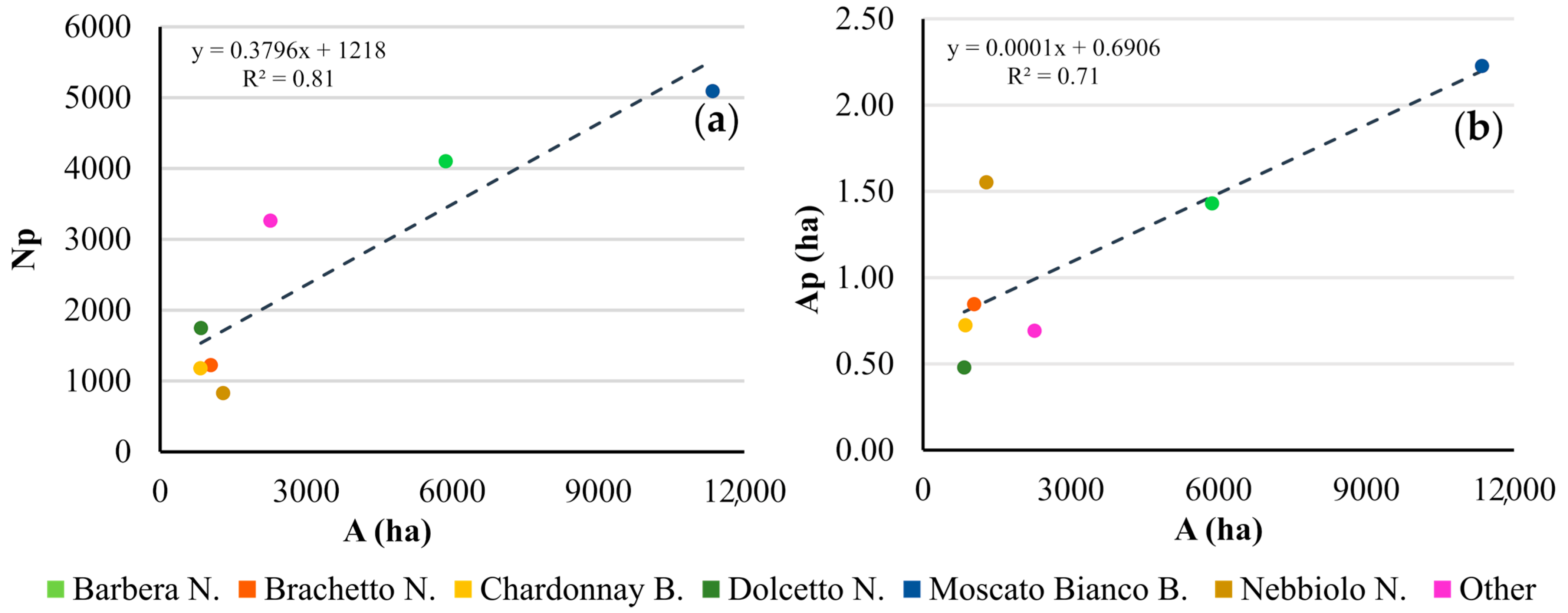
3.1. Analyzing Spatial Distribution of Grape Varieties

Six main grape varieties—namely, Barbera, Brachetto, Chardonnay, Dolcetto, Moscato Bianco, Nebbiolo, and other varieties—are present in the study area (Figure 2).

The number of vineyard parcels and the corresponding area were calculated for each grapevine variety (Figure 3a,b).

It was found that (Figure 3a,b): (i) 4102 parcels (23%) corresponding to about 5865 ha (25% in terms of area) are covered by Barbera, with an average parcel size of 1.43 ha; (ii) 1224 parcels (7%) corresponding to about 1039 ha (4%) are covered by Brachetto, with an average parcel size of 0.85 ha; (iii) 1184 parcels (7%) corresponding to about 857 ha (4% in terms of area) are covered by Chardonnay, with an average parcel size of 0.72 ha; (iv) 1747 parcels (10%) corresponding to about 836 ha (4% in terms of area) are covered by Dolcetto, with an average parcel size of 0.48 ha; (v) 5094 parcels (29%) corresponding to about 11,343 ha (48% in terms of area) are covered by Moscato Bianco Dolcetto, with an average parcel size of 2.2 ha; (vi) 829 parcels (5%) corresponding to about 1289 ha (5% in terms of area) are covered by Nebbiolo, with an average parcel size of 1.55 ha; and (vii) finally, other minor vine varieties cover a total of about 2261 ha (3262 parcels) with an average parcel size of 0.70 ha.

Comparing the total area (A) versus the number of parcels (Np) for each grape variety and the total area (A) versus the average parcel area size (Ap) per grape variety, some interesting relationships can be pointed out (Figure 4).

Figure 4a shows that the Np grows while A grows too, suggesting a moderate difference in the Ap between grape variety. Nevertheless, the Ap is somehow related to the A of each grape variety (Figure 4b), suggesting that more the grape variety is present, the higher the level of aggregation of the parcels. The only important exception comes from Nebbiolo which shows highly sized average parcels in spite of a reduced presence in the area.

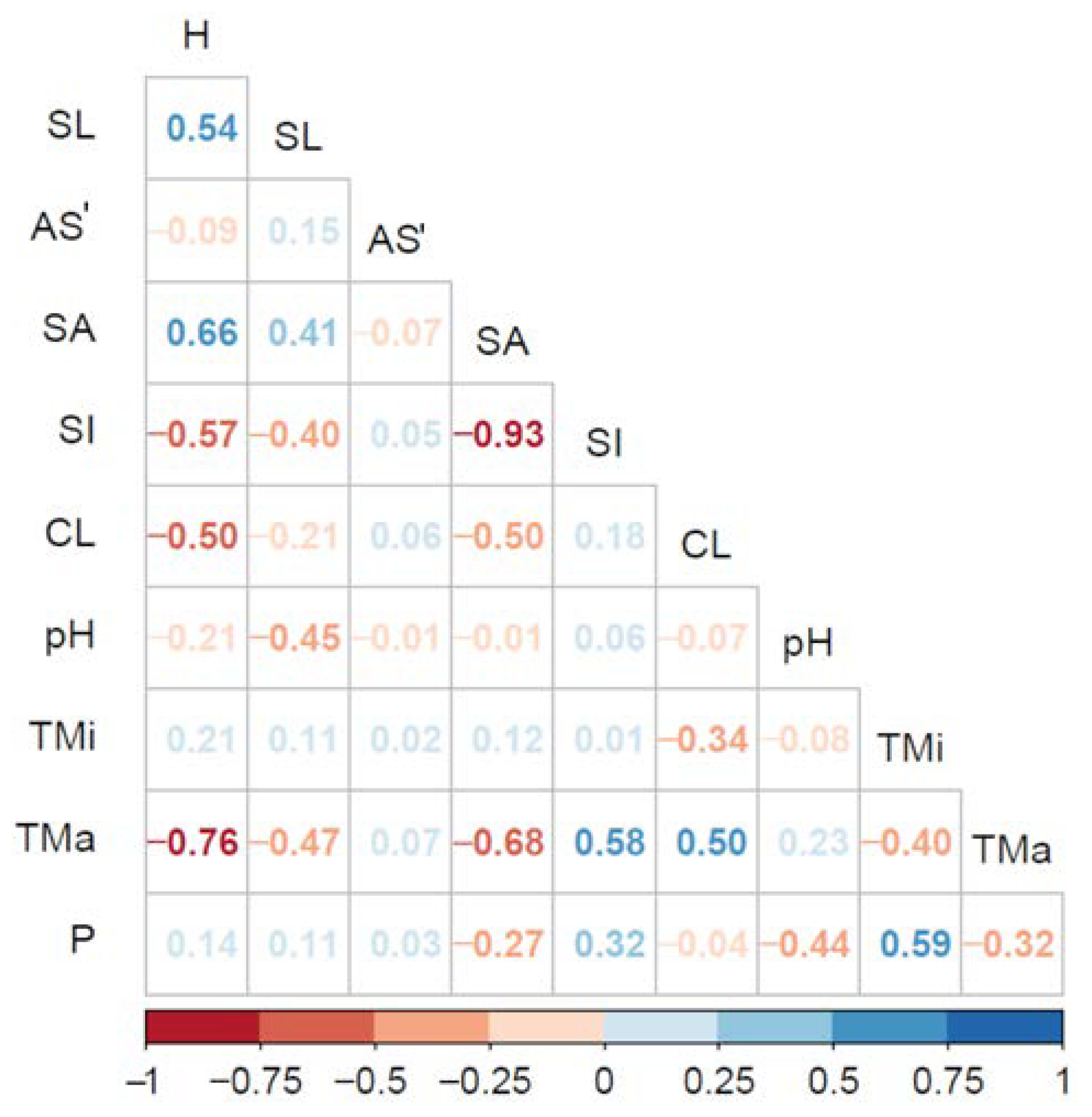
3.2. Data Pre-Processing

Concerning pedological data, after converting the original values (g/kg) for texture data to the corresponding mass percentages and the original values of pH to the normal scale of pH, data from the four available depth-dependent maps were averaged and oversampled to generate four raster layers representing the average mass percentage of sand, silt, and clay and the average pH of the first 60 cm of soil. Results are reported in Figure 5.

Concerning climate data, to map the average climatic conditions of the area, yearly values were averaged along the reference period obtaining three new raster layers (TMi, TMa, and P) with a grid size of 5 m. Results are reported in Figure 6.

As far as terrain morphology (topography) is concerned, the native DTM (H), slope (SL), and aspect layers (AS) were considered. In AOI, H ranges between about 103 and 734.15 m a.s.l., SL between 0° and 76°, and AS between 0 rad and 6.28 rad. If focusing on vineyards only, (i) H varies from 125 m a.s.l. to its maximum; (ii) SL ranges between 0° and 28°; and (iii) AS is always between 0 rad and 6.28 rad. Concerning topography, following the transformation of AS in AS′ (Equation (1)), the results are shown in Figure 7.

The pedological, climatic, and morphological raster layers were standardized, thus generating 10 new standardized raster maps (namely, SA_ST, SI_ST, CL_ST, pH_ST, TMi_ST, TMa_ST, P_ST, H_ST, SL_ST, and AS′_ST).

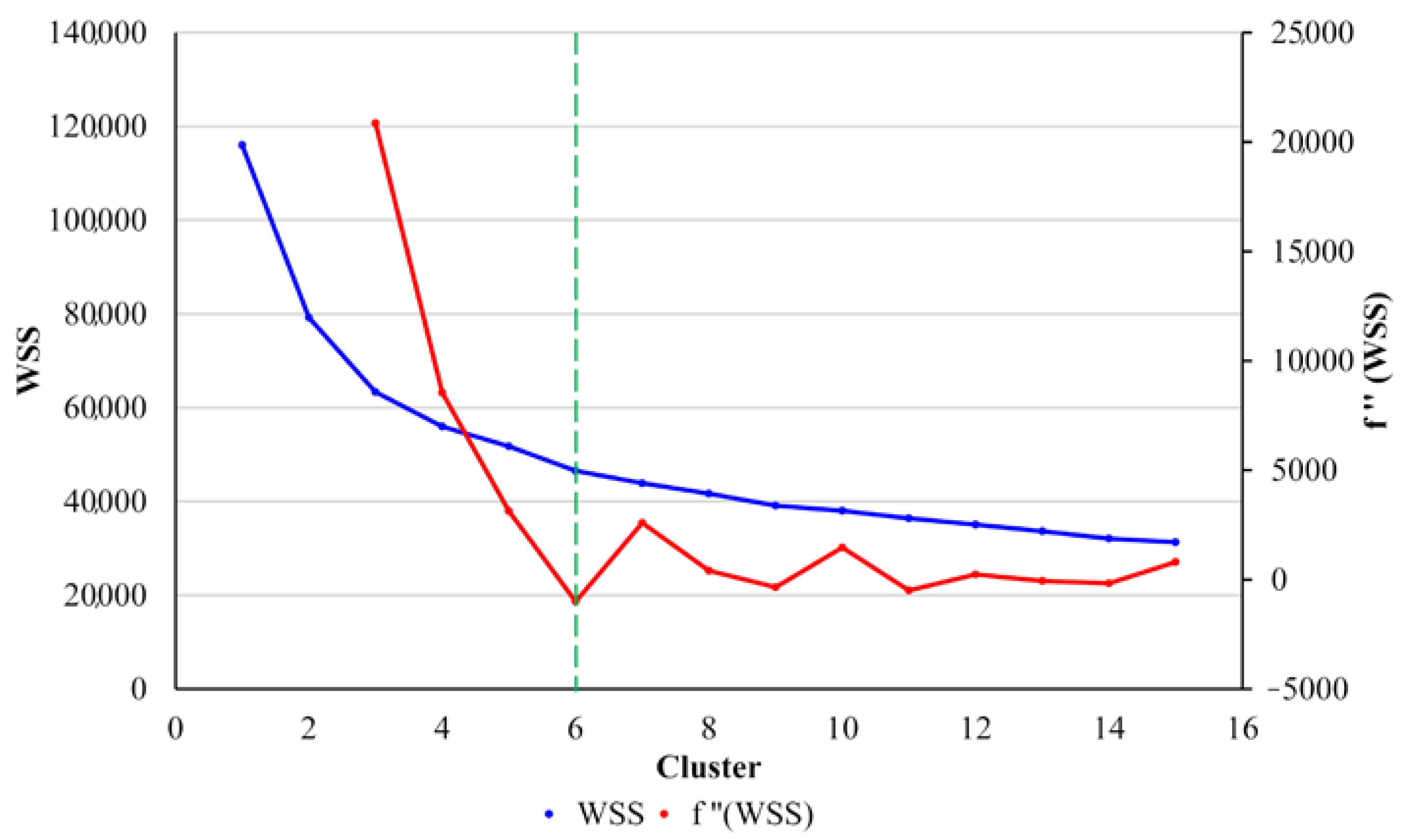
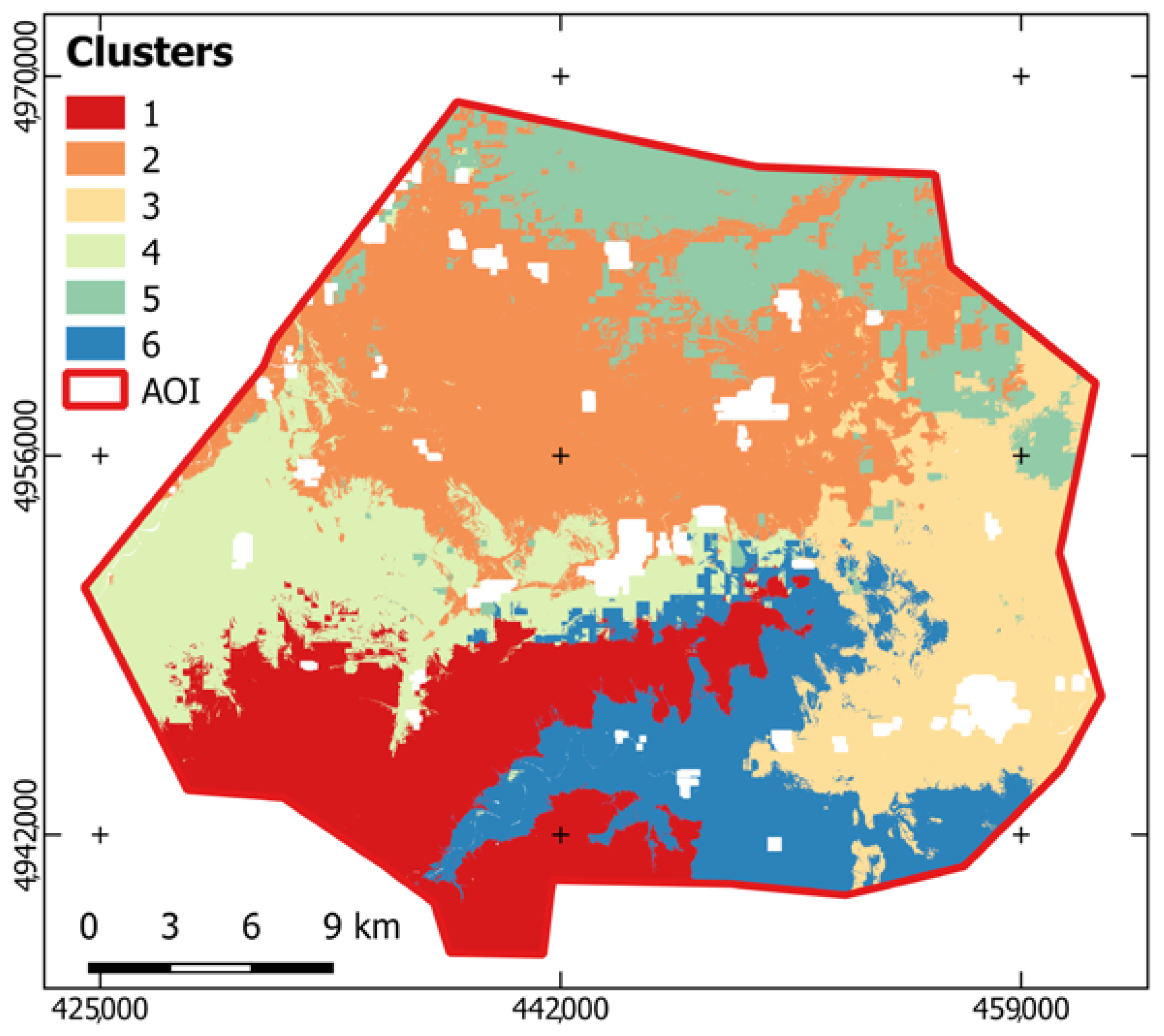
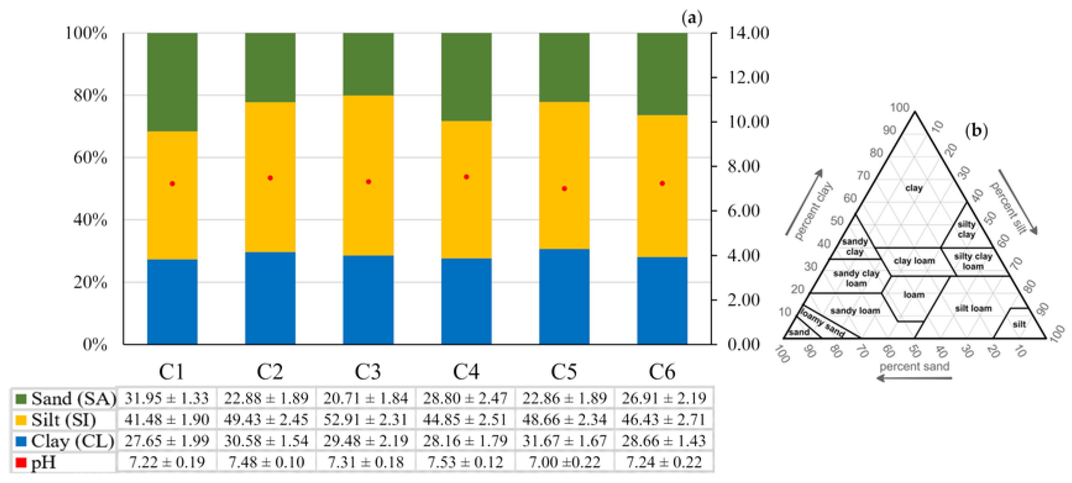
3.3. K-Means Clustering and Zonal Statistics Computation

A correlation analysis of all standardized values was performed and the results are shown in Figure 8.

This correlation analysis showed that: (i) most of the variables were not significantly correlated to each other, with Pearson’s r values of less than 0.5 in absolute value; (ii) SA has been proven to be negatively correlated with SI, since both, jointly with CL, are complementary for soil texture; (iii) H proved to be negatively correlated with TMa—in fact, it is known that as the altitude increases, the temperature decreases; and (iv) other variables are poorly correlated, as H and SA, SI and TMa, or TMi and P. The correlation analysis provides no information on whether the link is cause-and-effect. In spite of these exceptions, all of the input was considered during clustering.

To find the optimal number of clusters, the elbow method was used, adopting the second derivative (f’’) of the “sum of squares” function to make it explicit. The breaking point of f’’ was used as the one corresponding to the optimal number of clusters—six—to be used during clustering analysis. Results are shown in Figure 9.

The k-means clustering result is reported in Figure 10. The clustering result, supplied as a raster layer, was vectorized, and the corresponding zonal statistics (mean and standard deviation) computed for all the inputs.

The cluster size is reported in

Table 2. Cluster area size (ha and %) resulting from classification.

Cluster (C)	Area (ha)	Area (%)
C1	13,547.88	17.20
C2	22,339.15	28.36
C3	11,577.79	14.70
C4	11,301.25	14.35
C5	9690.65	12.30
C6	10,308.72	13.09

.

The statistics are reported in Figure 11 for the pedological features.

Figure 11a reports that all clusters show similar percentages of SA (20.71–31.95%), SI (41.48–52.91%), CL (27.65–31.67%), and pH value (7.00–7.53). Being a dimensionally limited area located in the same landscape, it is appropriate to assume that the geological origin and other major soil-forming factors may have low variability. Figure 11a confirms this fact, especially from a pedological point of view, which is slightly variable comparing the six clusters. All of the clusters, in fact, fall into the “clay loam” class as defined by the USDA (U.S. Department of Agriculture) soil texture triangle (Figure 11b) [68,69].

With reference to Equation (2), the significance of the among-cluster difference (Δ) was tested. For each feature (pedology, climate, and topography, respectively), the differences between the cluster are highlighted using a color code, where red and green show not significant and significant difference values, respectively. The results for the pedological feature are represented in Figure 12.

In spite of the apparently small differences among clusters in terms of pedological features, Figure 12 helps to read the following: (i) Clay content and pH are weak discriminants, showing not significant differences for most of the compared pairs. In particular, pH values prove that, in AOI, the soils are generally neutral ones (about 7 pH); i.e., they present a good nutritional balance proper for vine growth [70,71]. (ii) Both sand and silt show a good capability of separating clusters. This similar feature also confirms they are correlated as previously mentioned (Figure 8). (iii) C1 is significantly different from all other clusters both in terms of SA (highest values) and SI (lowest values). (iv) C2 and C5 are similar to each other for SA, SI, and CL, and weakly differ only for pH. (v) The C2 and C4 areas are the “most” alkaline ones compared with the other clusters. (vi) C3 is significantly different from all other clusters in terms of SI, presenting the highest silt content.

As far as climatic features are concerned, the cluster mean and standard deviation values are reported in

Table 3. Statistics concerning climatic features of clusters—minimum temperature (TMi, °C), maximum temperature (TMa, °C), and cumulative precipitation (P, mm/year).

Cluster (C)	Minimum Temperature— TMi (°C)	Maximum Temperature— TMa (°C)	Cumulative Precipitation— P (mm/year)
C1	0.14 ± 0.18	28.50 ± 0.39	638.89 ± 23.63
C2	−0.07 ± 0.11	29.95 ± 0.15	598.28 ± 38.40
C3	0.34 ± 0.26	29.55 ± 0.25	702.53 ± 22.97
C4	0.04 ± 0.15	29.52 ± 0.40	574.95 ± 28.86
C5	−0.18 ± 0.13	29.85 ± 0.14	628.48 ± 39.16
C6	0.49 ± 0.23	29.00 ± 0.29	671.73 ± 34.34

.

Weaker differences among clusters can be found while looking at the climatic data as reported in Table 3, which show the following range of variability for TMi, TMa, and P, respectively: −0.18–+0.34 °C, +28.50–+29.95 °C, and 574.95–702.53 mm/year.

The most significant differences can be observed for precipitation. These range between a minimum of about 10 mm/year (C1 and C5) to a maximum of about 130 mm/year (C3 and C4). In particular, C2 and C4 correspond to the driest conditions (averagely 586 mm/year), C1 and C5 to the average ones (averagely 629 mm/year, i.e., +6.7%), and C3 and C6 to the wettest ones (averagely 687 mm/year, i.e., +19%).

The results regarding the significance of the among-cluster difference for the climatic feature are represented in Figure 13.

After testing the significance of the cluster differences (Figure 13), it was found that: (i) C6 (highest values) and C5 (lowest values) differ from all the other clusters in terms of TMi, with the only exception of C3 and C2, respectively. (ii) TMa is the climatic feature showing the strongest capability of differentiating clusters. In particular, the C1 and C6 areas behave significantly different from the other clusters C5 and C2. (iii) Half-a-degree Celsius appears to be enough to differentiate thermal conditions in the area. (iv) C3 (highest values) and C4 (lowest values) differ from all the other clusters in terms of P, with the only exception being C6 and C2, respectively.

As far as topographic features are concerned, the cluster mean and standard deviation values are reported in

Table 4. Statistics concerning topographic features of clusters—altitude (H), slope (SL), and transformed aspect (AS′). NW = North-West-looking slopes with no dominance of both N and W; NE = North-East-looking slopes with no dominance of both N and E; NNW = North-West-looking slopes with dominance of N; NNE = North-East-looking slopes with dominance of N; NWW = North-West-looking slopes with dominance of W; NEE = North-East-looking slopes with dominance of E; SW = South-West-looking slopes with no dominance of both S and W; SE = South-East-looking slopes with no dominance of both S and E; SSW = South-West-looking slopes with dominance of S; SSE = South-East-looking slopes with dominance of S; SWW = South-West-looking slopes with dominance of W; and SEE = South-East-looking slopes with dominance of E.

Cluster (C)	Altitude—H (m a.s.l.)	Slope—SL (°)	Transformed Aspect—AS′ (Dimensionless)
C1	435.87 ± 87.47	20.55 ± 8.34	0.83 ± 0.69 (NWW/NEE)
C2	193.30 ± 45.67	8.63 ± 5.31	0.88 ± 0.69 (NWW/NEE)
C3	235.22 ± 60.18	11.51 ± 7.91	0.93 ± 0.70 (NWW/NEE)
C4	273.80 ± 73.01	15.22 ± 8.84	0.81 ± 0.66 (NWW/NEE)
C5	190.01 ± 36.72	17.04 ± 6.42	0.96 ± 0.70 (NWW/NEE)
C6	295.07 ± 77.07	17.18 ± 6.56	0.91 ± 0.68 (NWW/NEE)

.

While analyzing the topographic features (Table 4), it can be noticed that C1 and C2 define opposite conditions: C1 is characterized by the highest values of altitude and slope (436 m a.s.l. and 20°.55, respectively), while C2 is characterized by the lowest ones (193 m a.s.l. and 8°.63, respectively).

C5 and C6 are characterized by similar average slope values (17°.04 and 17°.18, respectively) and significantly differ in altitude (190.01 and 295.07 m a.s.l.).

Aspect appears to be ineffective in discriminating among clusters. As shown in Table 4, the results demonstrate that vineyards are located in parcels with a similar aspect (mainly the NWW/NEE aspect). This cannot be assumed as a general conclusion, since aspect is known to influence local sun-lighting conditions to which vines are sensitive. Conversely, it is certainly related to the homogeneous conditions of hill slopes in AOI that are well-known to be prevalently East–West-looking.

The results regarding the significance of the among-cluster difference for the topographical feature are represented in Figure 14.

After testing the significance of the cluster differences in terms of topographic features (Figure 14), it was found that: (i) only altitude appears to be able to significantly discriminate between clusters; (ii) altitude is significantly different among the clusters; (iii) C1 is significantly different from all other clusters for altitude (highest values) and from C2, C5, and C6 for slope; and (iv) aspect-related effects appear to be negligible in the area.

As far as the investigation about possible dependencies of vine varieties from the zones (clusters) is concerned, the following interpretation keys were adopted from the obtained results, reporting some discussions for each feature analyzed. The significance of the differences in the soil-topographic and climatic characteristics of the zones (clusters) was analyzed and the results were compared with the well-known optimal conditions for vine growth, in order to highlight some essential differences.

As far as pedology is concerned, all soils in the area fall into the clay loam” USDA class where the high fertility of loamy soils is coupled with a good water capacity due to the clay fraction [72]. Clay loamy soils are considered among the most fertile soils, as the clay component provides excellent macro- and micro-nutrient availability and the clay component, generally, affects water retention, preventing grapevine water stress during the summer season and dangerous waterlogging during the winter season [72]. Regarding pH, neutral values (pH around 7) define the optimal balance of nutrient availability for plants to occur.

As far as climatic factors are concerned, it has to be remarked that they are related to the health status of crops; the phenological stages of the growing cycle, precipitation, and temperatures are closely related to each other [73]. The maximum temperatures are typically reached in the warm season (July–August). In the delicate flowering phase (May–June), the average temperatures typically vary close to the optimal values for grapevine development, significantly lower than the maximum temperature. The flowering phase is also delicate in terms of precipitation: if it is too excessive, it can affect subsequent phenological stages [74]. Typically, in AOI, the season characterized by repetitive rainfall does not coincide with the vine flowering phase. Minimum temperatures are typical of the cold season (December–January), when the plant is in vegetative rest until the following spring. The minimum temperatures shown in Table 3 do not cause unfavorable conditions for vine growth.

As far as topography is concerned: (i) the altitude certainly conditions the air temperature; (ii) the slope aspect influences the intercepted solar radiation; and (iii) the slope steepness conditions the accessibility and Sun insolation, as well. Moreover, the relationship linking the slope and soils is well-known [75]. In particular, steep slopes having clay loam soils can provide advantages and disadvantages. As far as water accumulation is concerned, the clay fraction of loamy soils can favour it, determining unfavourable conditions for vines. Conversely, a high slope supports superficial water flow, limiting water stagnation.

Additionally, the slope can affect cold air drainage in the vineyard, which represents a very important parameter for protecting vines from the spring frost. In fact, a high slope could result in a faster movement of cold air from the top to the base of the vineyard. With these premises, the steepest slopes with clay loam soils should provide better conditions for vines.

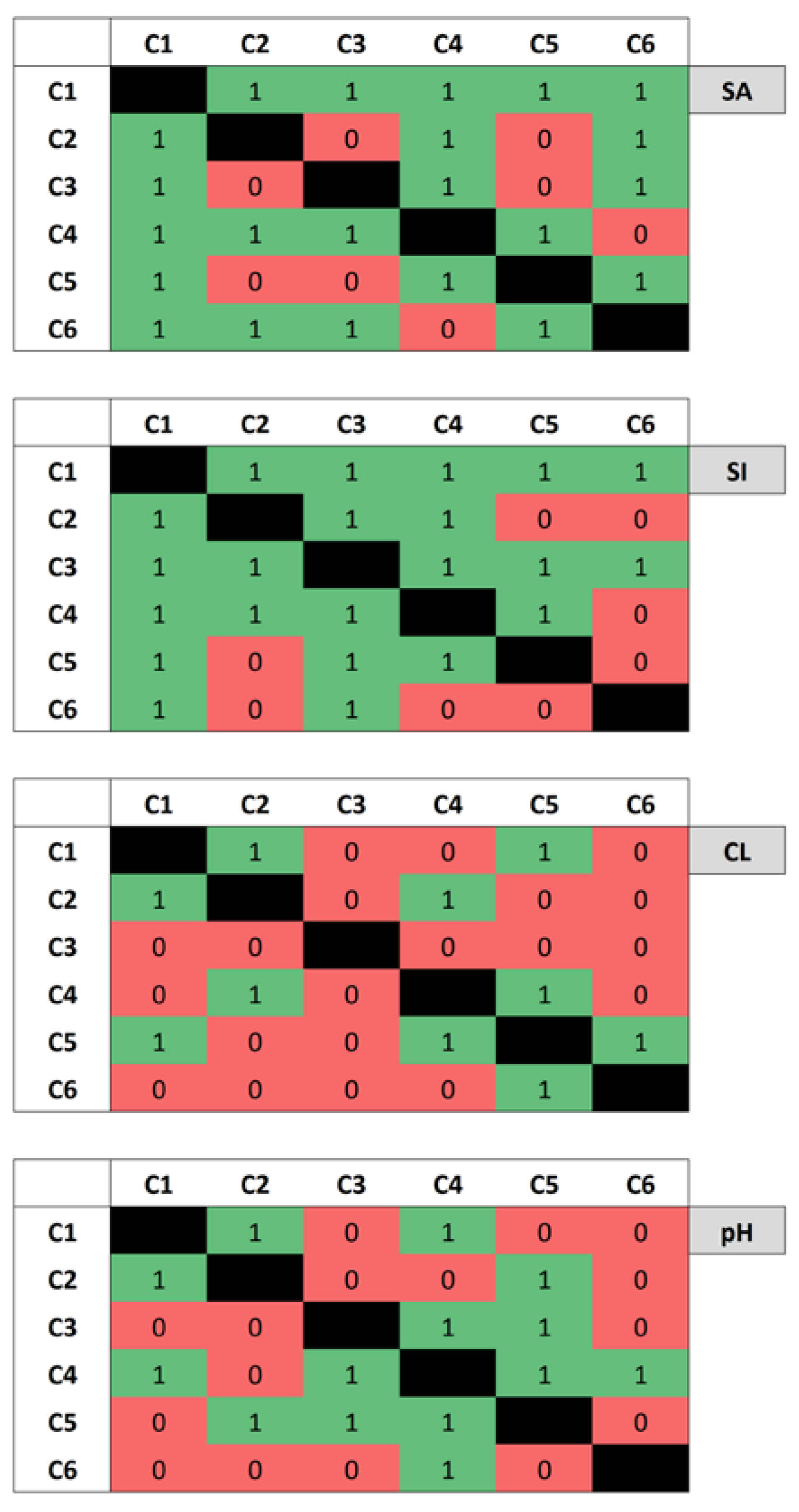
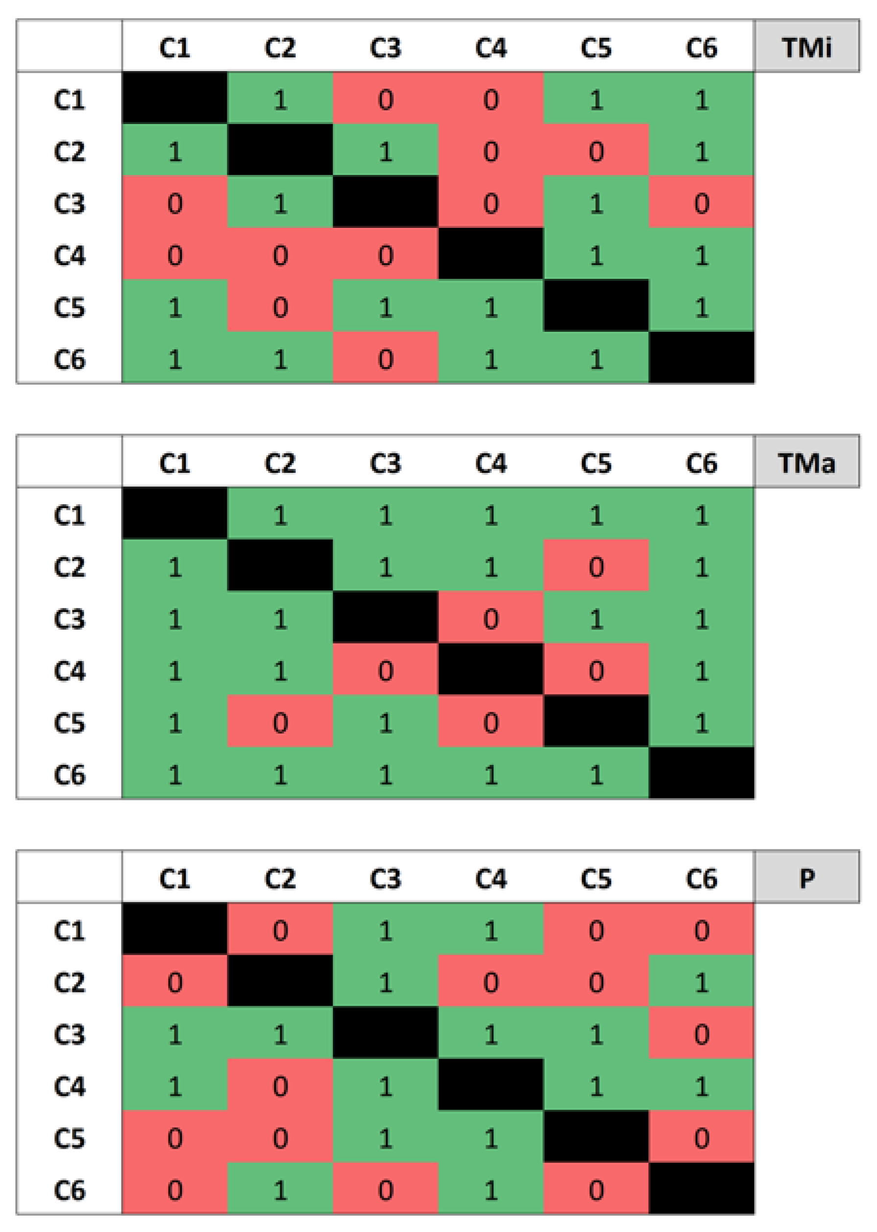
3.4. Analyzing Grape Variety Dependence from Zones

In this work, the obtained clusters were analyzed versus grape variety to verify eventual dependencies through the computation of occurrences of vine varieties within each cluster. Results are reported in Figure 15.

Assuming that the driving factor for interpretation was the vine grape variety, we tested its occurrence within the clusters, looking for an eventual specificity that made one cluster preferable against the others. In particular, with reference to Figure 15a,b, it can be noticed that C2, C3, and C4 are, in general, the clusters that majorly host vines.

The “Barbera” grape variety appears to be majorly located in C2, about 67% in terms of area (3939 ha) and about 50% in terms of number of parcels (2058).

The “Brachetto N.” grape variety appears to be majorly located in C3, about 48% in terms of area (494 ha) and about 43% in terms of number of parcels (529), with a significant contribution of cluster C2 which represents the 22% (228 ha) and 23% (286) of the whole in terms of area and number of parcels, respectively.

The “Chardonnay B.” grape variety appears to be distributed in C1, C2, C3, and C4, which represent 22% (185 ha), 35% (301 ha), 15% (128 ha), and 16% (137 ha) of the whole, respectively, in terms of area, and 18% (211), 39% (462), 12% (140), and 20% (237), respectively, in terms of number of parcels.

Similarly, the “Dolcetto N.” grape variety appears to be distributed in C1, C2, C3, and C4, which represent 22% (181 ha), 23% (192 ha), 18% (153 ha), and 28% (234 ha) of the whole, respectively, in terms of area, and 19% (334), 27% (473), 14% (248), and 30% (533), respectively, in terms of number of parcels.

Again, the “Moscato Bianco B.” grape variety appears to be significantly distributed in C1, C2, C3, and C4, which represent 24% (2710 ha), 20% (2231 ha), 15% (1751 ha), and 32% (3634 ha) of the whole, respectively, in terms of area, and 24% (1230), 24% (1238), 13% (689), and 24% (1212), respectively, in terms of number of parcels.

In the “Nebbiolo N.” vine variety, the C4 is strongly prevalent with a percentage of about 82% in terms of area (1056 ha) and 485 parcels (58.50% of total), suggesting a major specificity that this type of grape variety requires.

Finally, other varieties distribute over C1, C2, C3, and C4, with percentages ranging from 14% to 43% (321, 966, 346, and 323 ha, respectively), considering the area size value, and from 12% to 46% (405, 1490, 472, and 561, respectively), considering the number of parcels.

Surprisingly, C5 and C6 proved to be the less appealing clusters for viticulture. They size about the 12% (9690 ha) and 13% (10308 ha) of the total (vineyards and other land use classes) AOI, respectively. Nevertheless, while comparing vine occurrence within C5 and C6, we found that only 667 ha (7%) and 1710 ha (about 16 %) are devoted to grape cultivation, respectively. These percentages, if referring to the vineyard area in AOI (about 23490 ha), correspond to 3% and 7% of the whole, for C5 and C6, respectively.

In spite of this unfavorable situation, it cannot be definitely asserted that the C5 and C6 clusters are not suitable for hosting vines. In fact, they are not particularly small compared with the other clusters. Pedology cannot be a justification, since both C5 and C6 fall into the “clay loam” USDA class, which is characterized by an excellent content of silt and a rather important fraction of clay that is known to determine suitable conditions for viticulture, nor climatic conditions, since they appear to be similar to the ones from other clusters. Similarly, the topographic features of C5 and C6 do not suggest any evident unfavorable condition compared with the other clusters.

One of the reasons for this result can possibly rely on the reference dataset we used to locate vineyards in the area, i.e., the regional Agriculture Register service (provisions of D.P.R. 503/1999). It is worth a reminder that this dataset only reports information about those parcels that somehow have undergone an administrative process within the EU CAP framework with the public administration. They, therefore, correspond to vineyards cultivated by viticultural entrepreneurs and neglect eventual parcels belonging to small private family-run farms. They certainly represent the local commerce-devoted viticultural context well, but are unable to include familial properties.

A second reason can be recognized in the historical colonization of the area. Looking at Figure 10, it is possible to notice that clusters C5 and C6 are those where urbanized areas (white holes) are absent (9.6% and 1.6% of the total cluster area, respectively, considering the dataset of the Land Cover Piemonte project [76]). Consequently, a topological motivation related to the local urbanization model can be somehow hypothesized to partially explain the exception of C5 and C6. People, in fact, tend to exploit those areas closest to their houses and easiest to be accessed.

Additionally, the Land Cover Piemonte map shows that about 55% and 47% of C5 and C6, respectively, are covered by forest or abandoned land. This fosters the idea that these areas are and probably have always been marginal.

Some further investigations will be performed in future to test this hypothesis.

Comparing the results with others works, the following actually came out: (i) Most of the authors aimed to directly map terroirs, thus introducing a more advanced step. Our aim was "zone" identification, since the subsequent step (terroir identification) requires specific non-open and non-free data directly related to product identity and quality. (ii) Many works included multispectral remotely sensed data, in order to relate zoning to the vegetative behavior of the imaged vineyards, with no specific focus on open and free data (see [19,20]). (iii) This is the first work reporting the experience in our study area not in terms of “terroirs”, nor of “zones”.

The methodology proposed in this work represents a useful step towards a global vineyard zonation, which could be assumed as the starting “objective” point to finally recognize (and commercialize) the “terroir” label. Moreover, given the slightly simple workflow, our procedure will permit farmers that are unskilled with data and complicated elaborations (e.g., satellite image processing) to manage familiar information useful for vineyard management, in a simple and easy way. This will permit them to easily interpret possible relationships among those territorial features with grape varieties.

Being that the methodology proposed a propaedeutic map to the identification of terroirs, it can present multiple added values. In fact, it makes it possible: (i) to characterize a valuable wine-production area (NW-Italy); (ii) to ignite a new service for local winemakers to address their commercial policies; (iii) to point out the relationships among pedo-topological and climatic conditions and local grape varieties, possibly supporting the identification of areas to extend cultivation; and (iv) to reproduce similar results worldwide, being that most of the used data are global and free.

4. Conclusions

The possibility of recognizing and mapping local specificities of a wine-production area is highly desirable, as environmental conditions are the main drivers of wine-production in terms of both quality and quantity.

Terroir mapping based on a traditional methodology would require considerable investments of time and money by producers and wine consortia and would result in a subjective solution. For these reasons, this work proposes a GIS-based approach based on open and global data to zone a wine-production area located in Piemonte (NW Italy). In particular, AOI was investigated with the aim of developing, interpreting, and proposing zonation based on pedological (texture and chemical soil properties), climatic (temperature and precipitation), and morphological (altitude, slope, and aspect) discriminants with respect to different vine cultivars, aiming at proposing a repeatable and user-friendly procedure. It is worth highlighting that the obtained map is not a map of terroirs, but it is propaedeutic to their definition.

Some remarks can be also given about the repeatability of the proposed method in other areas around the world. This is guaranteed by the adoption of global open data that can be obtained for all countries: global DTMs are in fact available for free from many open archives (e.g., SRTM DEM [77,78] and ASTER DEM ([77,79]). SoilGrids and WorldClim data are global datasets.

Moreover, the approach proved to be able to generate a proper zonation, with significantly lower costs compared to more traditional methodologies applied in viticulture, that ordinarily require many man-hours for ground campaigns.

It is worth reminding, once more, that wine feature analyses and tasting sessions from local wineries still need to translate zones into the corresponding terroirs, thus leaving a significant degree of characterization related to the tasting itself, bottle aging, and peculiar imprints that wine producers may provide to their own production. Despite this latter factor, there are still issues surrounding the definition of terroir, which is certainly related to areas that are internally homogeneous with respect to those environmental characteristics that are expected to condition the production and quality of grape varieties; we expect that the proposed approach could somehow mitigate it.

Future developments of the methodology will be addressed to integrate new wine-related discriminants and to improve the geometric resolution of spatial variables. Future developments will be performed by analyzing the results using regional data and by extending the analyses, integrating more data such as soil nutrient abundance.

We can finally state that the scale of this work appears to be a proper compromise among cost, accuracy, and applicability, and zones can be somehow accepted as proto-terroirs.

References

1. Vrignon-Brenas, S.; Metay, A.; Leporatti, R.; Gharibi, S.; Fraga, A.; Dauzat, M.; Rolland, G.; Pellegrino, A. Gradual Responses of Grapevine Yield Components and Carbon Status to Nitrogen Supply. OENO One 2019, 53, 289–306. [Google Scholar] [CrossRef]
2. Duchêne, E.; Schneider, C.; Gaudillere, J.P. Effects of Nitrogen Nutrition Timing on Fruit Set of Grapevine, Cv. Grenache. Vitis-Geilweilerhof 2001, 40, 45–46. [Google Scholar]
3. Verdenal, T.; Dienes-Nagy, Á.; Spangenberg, J.E.; Zufferey, V.; Spring, J.-L.; Viret, O.; Marin-Carbonne, J.; van Leeuwen, C. Understanding and Managing Nitrogen Nutrition in Grapevine: A Review. OENO One 2021, 55, 3866. [Google Scholar] [CrossRef]
4. Cardoso, A.S.; Alonso, J.; Rodrigues, A.S.; Araújo-Paredes, C.; Mendes, S.; Valín, M.I. Agro-Ecological Terroir Units in the North West Iberian Peninsula Wine Regions. Appl. Geogr. 2019, 107, 51–62. [Google Scholar] [CrossRef]
5. Vaudour, E.; Leclercq, L.; Gilliot, J.-M.; Chaignon, B. Retrospective 70 Y-Spatial Analysis of Repeated Vine Mortality Patterns Using Ancient Aerial Time Series, Pléiades Images and Multi-Source Spatial and Field Data. Int. J. Appl. Earth Obs. Geoinf. 2017, 58, 234–248. [Google Scholar] [CrossRef]
6. Sarvia, F.; Petris, S.D.; Borgogno-Mondino, E. A Methodological Proposal to Support Estimation of Damages from Hailstorms Based on Copernicus Sentinel 2 Data Times Series. In Proceedings of the International Conference on Computational Science and Its Applications, Cagliari, Italy, 1–4 July 2020; Springer: Berlin/Heidelberg, Germany; pp. 737–751. [Google Scholar]
7. Sarvia, F.; De Petris, S.; Borgogno-Mondino, E. Mapping Ecological Focus Areas within the EU CAP Controls Framework by Copernicus Sentinel-2 Data. Agronomy 2022, 12, 406. [Google Scholar] [CrossRef]
8. Sarvia, F.; De Petris, S.; Borgogno-Mondino, E. Remotely Sensed Data to Support Insurance Strategies in Agriculture. In Proceedings of the Remote Sensing for Agriculture, Ecosystems, and Hydrology XXI, Strasbourg, France, 9–11 September 2019; SPIE: Bellingham, WA, USA, 2019; Volume 11149, pp. 438–448. [Google Scholar]
9. De Petris, S.; Sarvia, F.; Borgogno-Mondino, E. RPAS-Based Photogrammetry to Support Tree Stability Assessment: Longing for Precision Arboriculture. Urban For. Urban Green. 2020, 55, 126862. [Google Scholar] [CrossRef]
10. González, P.A.; Dans, E.P. The’terroirist’social Movement: The Reawakening of Wine Culture in Spain. J. Rural. Stud. 2018, 61, 184–196. [Google Scholar] [CrossRef]
11. Van Leeuwen, C.; Seguin, G. The Concept of Terroir in Viticulture. J. Wine Res. 2006, 17, 1–10. [Google Scholar] [CrossRef]
12. Van Leeuwen, C.; Roby, J.P.; De Resseguier, L. Soil-Related Terroir Factors: A Review. OENO One 2018, 52, 173–188. [Google Scholar] [CrossRef] [Green Version]
13. Priori, S.; Barbetti, R.; L’Abate, G.; Bucelli, P.; Storchi, P.; Costantini, E.A. Natural Terroir Units, Siena Province, Tuscany. J. Maps 2014, 10, 466–477. [Google Scholar] [CrossRef] [Green Version]
14. Sánchez, Y.; Martínez-Graña, A.M.; Santos-Francés, F.; Yenes, M. Index for the Calculation of Future Wine Areas According to Climate Change Application to the Protected Designation of Origin “Sierra de Salamanca” (Spain). Ecol. Indic. 2019, 107, 105646. [Google Scholar] [CrossRef]
15. Honorio, F.; García-Martín, A.; Moral, F.J.; Paniagua, L.L.; Rebollo, F.J. Spanish Vineyard Classification According to Bioclimatic Indexes. Aust. J. Grape Wine Res. 2018, 24, 335–344. [Google Scholar] [CrossRef]
16. Karoglan, M.; Prtenjak, M.T.; Šimon, S.; Osrečak, M.; Anić, M.; Kontić, J.K.; Andabaka, Ž.; Tomaz, I.; Grisogono, B.; Belušić, A. Classification of Croatian Winegrowing Regions Based on Bioclimatic Indices. In Proceedings of the E3S Web of Conferences, Moscow, Russia, 3–5 December 2018; EDP Sciences: Les Ulis, France, 2018; Volume 50, p. 01032. [Google Scholar]
17. Rieutort, L. Terroir. Hypergeo 2012, 1–2. Available online: http://geopuc.geo.puc-rio.br/media/v12n22a3-%20SARANTAKOS%20D.pdf (accessed on 27 October 2022).
18. Demossier, M. Beyond Terroir: Territorial Construction, Hegemonic Discourses, and French Wine Culture. J. R. Anthropol. Inst. 2011, 17, 685–705. [Google Scholar] [CrossRef]
19. Vaudour, E.; Carey, V.A.; Gilliot, J.-M. Digital Zoning of South African Viticultural Terroirs Using Bootstrapped Decision Trees on Morphometric Data and Multitemporal SPOT Images. Remote Sens. Environ. 2010, 114, 2940–2950. [Google Scholar] [CrossRef]
20. Martínez, A.; Gomez-Miguel, V.D. Vegetation Index Cartography as a Methodology Complement to the Terroir Zoning for Its Use in Precision Viticulture. OENO One 2017, 51, 289. [Google Scholar] [CrossRef] [Green Version]
21. Moral, F.J.; Rebollo, F.J.; Paniagua, L.L.; García-Martín, A. A GIS-Based Multivariate Clustering for Characterization and Ecoregion Mapping from a Viticultural Perspective. Span. J. Agric. Res. 2016, 14, e0206. [Google Scholar] [CrossRef]
22. Madruga, J.; Azevedo, E.B.; Sampaio, J.F.; Fernandes, F.; Reis, F.; Pinheiro, J. Analysis and Definition of Potential New Areas for Viticulture in the Azores (Portugal). Soil 2015, 1, 515–526. [Google Scholar] [CrossRef] [Green Version]
23. Irimia, L.M.; Patriche, C.V.; Quénol, H. Analysis of Viticultural Potential and Delineation of Homogeneous Viticultural Zones in a Temperate Climate Region of Romania. OENO One 2014, 48, 145–167. [Google Scholar] [CrossRef]
24. Bramley, R.G.V.; Gardiner, P.S. Underpinning Terroir with Data: A Quantitative Analysis of Biophysical Variation in the Margaret River Region of Western Australia. Aust. J. Grape Wine Res. 2021, 27, 420–430. [Google Scholar] [CrossRef]
25. Bramley, R.G.; Ouzman, J.; Trought, M.C. Making Sense of a Sense of Place: Precision Viticulture Approaches to the Analysis of Terroir at Different Scales: This Article Is Published in Cooperation with the XIIIth International Terroir Congress November 17–18 2020, Adelaide, Australia. Guest Editors: Cassandra Collins and Roberta De Bei. OENO One 2020, 54, 903–917. [Google Scholar]
26. Sanga-Ngoie, K.; Kumara, K.J.C.; Kobayashi, S. Potential Grape–Growing Sites in the Tropics: Exploration and Zoning Using a Gis Multi-Criteria Evaluation Approach. Proc. Asian Assoc. Remote Sens. 2010, 6. [Google Scholar]
27. Bramley, R.G.V.; Ouzman, J. Underpinning Terroir with Data: On What Grounds Might Subregionalisation of the Barossa Zone Geographical Indication Be Justified? Aust. J. Grape Wine Res. 2022, 28, 196–207. [Google Scholar] [CrossRef]
28. Failla, O.; Mariani, L.; Brancadoro, L.; Minelli, R.; Scienza, A.; Murada, G.; Mancini, S. Spatial Distribution of Solar Radiation and Its Effects on Vine Phenology and Grape Ripening in an Alpine Environment. Am. J. Enol. Vitic. 2004, 55, 128–138. [Google Scholar] [CrossRef]
29. Fraga, H.; Costa, R.; Santos, J. Modelling the Terroir of the Douro Demarcated Region, Portugal. In Proceedings of the E3S Web of Conferences, Moscow, Russia, 3–5 December 2018; EDP Sciences: Les Ulis, France, 2018; Volume 50, p. 02009. [Google Scholar]
30. Priori, S.; Valboa, G.; Pellegrini, S.; Perria, R.; Puccioni, S.; Storchi, P.; Costantini, E.A. Scale Effect of Viticultural Zoning under Three Contrasting Vintages in Chianti Classico Area (Tuscany, Italy). In Proceedings of the E3S Web of Conferences, Moscow, Russia, 3–5 December 2018; EDP Sciences: Les Ulis, France, 2018; Volume 50, p. 02012. [Google Scholar]
31. Mackenzie, D.E.; Christy, A.G. The Role of Soil Chemistry in Wine Grape Quality and Sustainable Soil Management in Vineyards. Water Sci. Technol. 2005, 51, 27–37. [Google Scholar] [CrossRef] [PubMed]
32. Protano, G.; Rossi, S. Relationship between Soil Geochemistry and Grape Composition in Tuscany (Italy). J. Plant Nutr. Soil Sci. 2014, 177, 500–508. [Google Scholar] [CrossRef]
33. White, R.E. The Value of Soil Knowledge in Understanding Wine Terroir. Front. Environ. Sci. 2020, 8, 12. [Google Scholar] [CrossRef]
34. Reynolds, A.G.; Rezaei, J.H. Spatial Variability in Ontario Cabernet Franc Vineyards: I. Interrelationships among Soil Composition, Soil Texture, Soil and Vine Water Status. J. Appl. Hortic. 2014, 16, 3–23. [Google Scholar] [CrossRef] [Green Version]
35. Marciniak, M.; Reynolds, A.G.; Brown, R.; Jollineau, M.; Kotsaki, E. Applications of Geospatial Technologies to Understand Terroir Effects in an Ontario Riesling Vineyard. Am. J. Enol. Vitic. 2017, 68, 169–187. [Google Scholar] [CrossRef]
36. Morari, F.; Castrignanò, A.; Pagliarin, C. Application of Multivariate Geostatistics in Delineating Management Zones within a Gravelly Vineyard Using Geo-Electrical Sensors. Comput. Electron. Agric. 2009, 68, 97–107. [Google Scholar] [CrossRef]
37. Noble, A.C. Evaluation of Chardonnay Wines Obtained from Sites with Different Soil Compositions. Am. J. Enol. Vitic. 1979, 30, 214–217. [Google Scholar] [CrossRef]
38. Bramley, R.G.V.; Ouzman, J.; Boss, P.K. Variation in Vine Vigour, Grape Yield and Vineyard Soils and Topography as Indicators of Variation in the Chemical Composition of Grapes, Wine and Wine Sensory Attributes. Aust. J. Grape Wine Res. 2011, 17, 217–229. [Google Scholar] [CrossRef]
39. Jones, G. Climate and Terroir: Impacts of Climate Variability and Change on Wine. Geosci. Can. Repr. Ser. 2006, 9, 203–217. [Google Scholar]
40. Santos, J.A.; Fraga, H.; Malheiro, A.C.; Moutinho-Pereira, J.; Dinis, L.-T.; Correia, C.; Moriondo, M.; Leolini, L.; Dibari, C.; Costafreda-Aumedes, S.; et al. A Review of the Potential Climate Change Impacts and Adaptation Options for European Viticulture. Appl. Sci. 2020, 10, 3092. [Google Scholar] [CrossRef]
41. Jones, G.V. The Climate Component of Terroir. Elem. Int. Mag. Mineral. Geochem. Petrol. 2018, 14, 167–172. [Google Scholar] [CrossRef]
42. Jones, G.V.; White, M.A.; Cooper, O.R.; Storchmann, K. Climate Change and Global Wine Quality. Clim. Change 2005, 73, 319–343. [Google Scholar] [CrossRef]
43. Van Leeuwen, C.; Darriet, P. The Impact of Climate Change on Viticulture and Wine Quality. J. Wine Econ. 2016, 11, 150–167. [Google Scholar] [CrossRef] [Green Version]
44. Jurisic, M.; Stanisavljevic, A.; Plascak, I. Application of Geographic Information System (GIS) in the Selection of Vineyard Sites in Croatia. Bulg. J. Agric. Sci. 2010, 16, 235–242. [Google Scholar]
45. Hunter, J.J.; Volschenk, C.G.; Booyse, M. Vineyard Row Orientation and Grape Ripeness Level Effects on Vegetative and Reproductive Growth Characteristics of Vitis Vinifera L. Cv. Shiraz/101-14 Mgt. Eur. J. Agron. 2017, 84, 47–57. [Google Scholar] [CrossRef]
46. Strack, T.; Stoll, M. Implication of Row Orientation Changes on Fruit Parameters of Vitis Vinifera L. Cv. Riesling in Steep Slope Vineyards. Foods 2021, 10, 2682. [Google Scholar] [CrossRef]
47. Salata, S.; Ozkavaf-Senalp, S.; Velibeyoğlu, K.; Elburz, Z. Land Suitability Analysis for Vineyard Cultivation in the Izmir Metropolitan Area. Land 2022, 11, 416. [Google Scholar] [CrossRef]
48. ISTAT—Istituto Nazionale Di Statistica. Available online: https://www.istat.it/it/ (accessed on 27 October 2022).
49. ISMEA Mercati. Available online: https://www.ismeamercati.it/vino (accessed on 27 October 2022).
50. WineNews—The Pocket Wine Web Site in Italy. Available online: Https://winenews.it/it/ (accessed on 27 October 2022).
51. Vini Piemontesi—Storia, Vitigni, DOC, DOCG, Vini Famosi—Italy’s Finest Wines. Available online: https://italysfinestwines.it/vini-piemontesi/ (accessed on 27 October 2022).
52. RETEVINO DOP-IGP—Ismea Mercati. Available online: https://www.ismeamercati.it/retevino-dop-igp (accessed on 27 October 2022).
53. ASSOVINI—Associazione Nazionale Produttori Vinicoli e Turismo Del Vino. Available online: https://www.assovini.it/ (accessed on 27 October 2022).
54. CHM—Community Heritage Maps. Available online: https://www.communityheritagemaps.com/ (accessed on 27 October 2022).
55. Vineyards—The Vineyard Explorer—Piedmont Wine Map. Available online: https://vineyards.com/wine-map/italy/piedmont (accessed on 27 October 2022).
56. B\lażejczyk, K.; Baranowski, J.; Jendritzky, G.; B\lażejczyk, A.; Bröde, P.; Fiala, D. Regional Features of the Bioclimate of Central and Southern Europe against the Background of the Köppen-Geiger Climate Classification. Geogr. Pol. 2015, 88, 439–453. [Google Scholar] [CrossRef] [Green Version]
57. IGRAC—Internation Groundwater Resources Assessment Centre. Available online: https://www.un-igrac.org/ (accessed on 24 October 2022).
58. Geoportale Piemonte. Available online: https://www.geoportale.piemonte.it/cms/ (accessed on 18 March 2022).
59. Anagrafe Agricola Del Piemonte. Available online: https://servizi.regione.piemonte.it/catalogo/anagrafe-agricola-piemonte (accessed on 18 March 2022).
60. WorldClim. Available online: https://www.worldclim.org/ (accessed on 2 December 2022).
61. SoilGrids—ISRIC. Available online: https://soilgrids.org/ (accessed on 22 October 2022).
62. Borgogno Mondino, E.; Fissore, V.; Lessio, A.; Motta, R. Are the New Gridded DSM/DTMs of the Piemonte Region (Italy) Proper for Forestry? A Fast and Simple Approach for a Posteriori Metric Assessment. Iforest Biogeosciences For. 2016, 9, 901. [Google Scholar] [CrossRef] [Green Version]
63. Poggio, L.; De Sousa, L.M.; Batjes, N.H.; Heuvelink, G.; Kempen, B.; Ribeiro, E.; Rossiter, D. SoilGrids 2.0: Producing Soil Information for the Globe with Quantified Spatial Uncertainty. Soil 2021, 7, 217–240. [Google Scholar] [CrossRef]
64. Harris, I.; Jones, P.D.; Osborn, T.J.; Lister, D.H. Updated High-Resolution Grids of Monthly Climatic Observations–the CRU TS3. 10 Dataset. Int. J. Climatol. 2014, 34, 623–642. [Google Scholar] [CrossRef] [Green Version]
65. Khan, H.H.; Khan, A.; Ahmed, S.; Perrin, J. GIS-Based Impact Assessment of Land-Use Changes on Groundwater Quality: Study from a Rapidly Urbanizing Region of South India. Environ. Earth Sci. 2011, 63, 1289–1302. [Google Scholar] [CrossRef]
66. Forgy, E.W. Cluster Analysis of Multivariate Data: Efficiency versus Interpretability of Classifications. Biometrics 1965, 21, 768–769. [Google Scholar]
67. Clayman, C.L.; Srinivasan, S.M.; Sangwan, R.S. K-Means Clustering and Principal Components Analysis of Microarray Data of L1000 Landmark Genes. Procedia Comput. Sci. 2020, 168, 97–104. [Google Scholar] [CrossRef]
68. Groenendyk, D.G.; Ferré, T.P.; Thorp, K.R.; Rice, A.K. Hydrologic-Process-Based Soil Texture Classifications for Improved Visualization of Landscape Function. PLoS ONE 2015, 10, e0131299. [Google Scholar] [CrossRef] [Green Version]
69. USDA—U.S. Department of Agriculture. Available online: https://www.usda.gov/ (accessed on 5 November 2022).
70. Brown, D. Soil Sampling Vineyards and Guidelines for Interpreting the Soil Test Results. Michigan State University. 2013. Available online: https://www.canr.msu.edu/news/soil_sampling_vineyards_and_guidelines_for_interpreting_the_soil_test_resul (accessed on 16 January 2023).
71. Soil PH in Vineyards—GRAPES. Available online: https://grapes.extension.org/soil-ph-in-vineyards/ (accessed on 9 December 2022).
72. Bruand, A.; Tessier, D. Water Retention Properties of the Clay in Soils Developed on Clayey Sediments: Significance of Parent Material and Soil History. Eur. J. Soil Sci. 2000, 51, 679–688. [Google Scholar] [CrossRef]
73. Fasi Fenologiche Della Vite—Coltivazione Biologica. Available online: https://www.coltivazionebiologica.it/fasi-fenologiche-della-vite/ (accessed on 19 December 2022).
74. La Vite e Il Clima—Quattrocalici. Available online: https://www.quattrocalici.it/conoscere-il-vino/la-vite-clima/ (accessed on 19 December 2022).
75. Stafne, E. Vineyard Site Selection—GRAPES. 2019. Available online: https://grapes.extension.org/vineyard-site-selection/ (accessed on 24 October 2022).
76. Land Cover Piemonte. Available online: https://www.geoportale.piemonte.it/cms/progetti/land-cover-piemonte (accessed on 21 February 2023).
77. EarthExplorer USGS—U.S. Geological Survey. Available online: https://earthexplorer.usgs.gov/ (accessed on 10 November 2022).
78. SRTM—Shuttle Radar Topography Mission—USGS. Available online: https://www.usgs.gov/centers/eros/science/usgs-eros-archive-digital-elevation-shuttle-radar-topography-mission-srtm-1 (accessed on 10 November 2022).
79. ASTER GDEM—Advanced Spaceborne Thermal Emission and Reflection Radiometer (ASTER) Global Digital Elevation Model (GDEM)—EARTHDATA NASA. Available online: Https://www.earthdata.nasa.gov/news/new-aster-gdem (accessed on 10 November 2022).
Figure 1. AOI and vineyard distribution in the study area (Piemonte, NW-Italy). Reference frame is WGS 84 UTM zone 32N (EPSG: 32,632).
Land 12 00647 g001
Figure 2. Map showing spatial distribution of grape varieties in the study area. (EPSG: 32,632 WGS 84 UTM zone 32N).
Land 12 00647 g002
Figure 3. Percentage distribution of grape varieties in AOI: (a) number of parcels (%) of the main grapevine varieties (total parcels = 17,442); and (b) area size (%) of the main grapevine varieties (total area = about 23,490 ha).
Land 12 00647 g003
Figure 4. Spatial analysis of grape variety in AOI: (a) total area (A—ha) versus the number of parcels (Np) for each grape variety; and (b) total area (A—ha) versus the average parcel area size (Ap—ha) for each grape variety.
Land 12 00647 g004
Figure 5. Raster layers mapping soil textural features in the study area: (a) sand (SA—%); (b) silt (SI—%); (c) clay (CL—%); and (d) pH (dimensionless) (EPSG: 32,632, WGS 84/UTM zone 32N).
Land 12 00647 g005
Figure 6. Raster layers mapping climatic features in the study area: (a) average yearly minimum temperature (TMi—°C); (b) average yearly maximum temperature (TMa—°C); and (c) average yearly cumulated precipitation (P—mm/year). (EPSG: 32,632, WGS 84/UTM zone 32N).
Land 12 00647 g006
Figure 7. Maps of H (a), SL (b), and AS′ (c) raster layers in the study area. Reference frame is WGS 84 UTM zone 32N (EPSG: 32,632).
Land 12 00647 g007
Figure 8. Correlogram relating all the standardized values of considered discriminants.
Land 12 00647 g008
Figure 9. Total within-cluster sum of squares (WSS, blue line) and its second derivative (f″(WSS), red line). The optimal number of significantly different clusters was found to be six (dotted green line), corresponding to the breaking value of f″.
Land 12 00647 g009
Figure 10. Clusters from k-means. The optimal number in AOI was found to be 6. (EPSG: 32,632, WGS 84 UTM 32N).
Land 12 00647 g010
Figure 11. Characterization and pedological classification of soils: (a) pedological parameters, namely, sand (SA), silt (SI), clay (CL), and pH (pH) of the 6 clusters from k-means; and (b) USDA soil texture triangle useful for soil classification.
Land 12 00647 g011
Figure 12. Significance of differences between the cluster mean percentages of SA, SI, and CL content. Red and green cells show not significant and significant difference values.
Land 12 00647 g012
Figure 13. Significance of differences between the cluster mean values of TMi, TMa, and P. Red and green cells show not significant and significant difference values.
Land 12 00647 g013
Figure 14. Significance of differences between the cluster mean values of H, SL, and AS′. Red and green cells show not significant and significant difference values.
Land 12 00647 g014
Figure 15. Analyzing grape variety dependence from zones (clusters): (a)% distribution of clusters for grape variety (ha); and (b)% of parcels cultivated with a specific grape variety per cluster.
Land 12 00647 g015