Article

Assessment of Soil Potentially Toxic Metal Pollution in Kolchugino Town, Russia: Characteristics and Pollution

by
Inna Z. Kamanina
1,2,
Wael M. Badawy
2,3,*,
Svetlana P. Kaplina
4,
Oleg A. Makarov
5 and
Sergey V. Mamikhin
5
1
Department of Ecology and Earth Sciences, Faculty of Natural and Engineering Sciences, Dubna State University, 141980 Dubna, Russia
2
Frank Laboratory of Neutron Physics, Joint Institute for Nuclear Research, 141980 Dubna, Russia
3
Radiation Protection and Civil Defense Department, Nuclear Research Center, Egyptian Atomic Energy Authority, Cairo 13759, Egypt
4
Flerov Laboratory of Nuclear Reactions, Joint Institute for Nuclear Research, 141980 Dubna, Russia
5
Faculty of Soil Science, Lomonosov Moscow State University, 119991 Moscow, Russia
*
Author to whom correspondence should be addressed.
Land 2023, 12(2), 439; https://doi.org/10.3390/land12020439
Submission received: 14 January 2023 / Revised: 31 January 2023 / Accepted: 4 February 2023 / Published: 8 February 2023
(This article belongs to the Special Issue Monitoring Soil Properties Based on Remote Sensing)

Abstract

:
The present study was carried out to describe the characteristic features of potentially toxic metals (PTMs) in the soil of industrial city, Kolchugino–Vladimir Region–Russia. The mass fractions in mg/kg of Cu, Pb, Zn, and Cd were measured by atomic absorption spectrometer (AAS). Multivariate statistical analysis and hierarchical cluster analysis (HCA), were performed. The obtained results of the potentially toxic elements were mapped using ArcGIS. A total of four pollution indices were calculated to identify the areas with significant pollution associations. The data analysis showed that locations 14 (urban area) and 16 (non-ferrous metallurgy plant) contribute significantly to pollution. Maximum likelihood method was used to classify the land-use and land-cover (LULC). The analysis shows that locations 14 and 16 are belonging to the industrial area on LULC. Great attention should be paid to the control and regulation of waste disposal into the environment, which in turn, has an adversely impact on human health. By using the data, it could help to identify areas where waste control measures need to be implemented, such as increasing recycling or introducing more waste control legislation. It could also help to identify areas where waste control efforts have been successful. Data can be used by government, policymakers, and stakeholders for future planning and R&D activities.

1. Introduction

Soil contamination with potentially toxic metals (PTMs) is a growing concern due to the increasing of industrialization and urbanization worldwide. Recent literature suggests that toxic metal pollution is a widespread problem affecting both rural and urban areas, with serious consequences for human health, the environment, and ecosystem sustainability [1]. PTMs can enter the soil from various sources, including industrial waste, agricultural chemicals, and waste disposal sites. In urban areas, the use of leaded gasoline, pesticides, and fertilizers also contribute to soil contamination. In addition, it was shown that contaminated soils can lead to the accumulation of (PTMs) in crops and other food sources, resulting in exposure through the food chain. Eventually, it can lead to a range of adverse health effects, including cardiovascular disease, neurological damage, and developmental problems in children [2,3,4,5,6].
Quantitative measurement of soil trace metals is critical for studying the characteristics of soil quality and assessing the risks to human health associated with soil research. Environmentally relevant concentrations of heavy metals in soils have attracted the attention of government and regulatory agencies seeking to reduce human health risks associated with environmental pollution [7,8,9,10].
Pollution is the byproduct of human activities that can harm both people and nature. Many scientists have been concerned about the increasing levels of soil pollution and its effects on human health. Their concern prompted them to develop various pollution indices that can be used to measure the severity of soil pollution [11]. In this work, various pollution indices have been calculated to assess the soil quality and ecological situation in the surrounding environment.
The risk due to the elevated levels of (PTMs) is based on the fact that most elements have significant biological activity and their high mass fractions may pose a toxic effect. In addition, (PTMs) are readily biodegradable and accumulate in the biogeochemical cycle, so they are essentially not removed from the system.
In this context, continuous monitoring is a primary and very important task to assess the levels of (PTMs) in coastal soils and river sediments, especially in urbanized and industrial areas with high technogenic loads [12,13,14]. In this regard, the mass fractions of the elements in the environment are an important factor affecting regional health and longevity [15,16]. The excess or unbalanced distribution of elements in the soil, even if it is natural, may lead to various forms of the disease [15]. Furthermore, human activities such as mining, urbanization extension, construction, and the building have resulted in soil destruction [17,18].
The development of cities leads to the formation of a specific urban environment. Mostly, in large cities, the results of anthropogenic impact on natural processes are most evident. Therefore, numerous studies have been devoted to the analysis of their ecological situation. However, regarding small cities, there are only few works devoted to the ecology of small cities. They mainly explore socioeconomic problems which in turn, affect the ecology of small cities as well [19]. For instance, Kolchugino city, Vladimir Region–Russia is a residential city and industrial one as well. It has many factories and enterprises that remarkably affect the ecology of the city. Therefore, a total of four selected elements (Zn, Pb, Cu, and Cd) were measured in soil samples collected from an industrial city, Kolchugino, using atomic absorption spectrometer (AAS). AAS is a widely used analytical technique for determining the concentrations of elements in soil samples.
The main objectives of the current work are: (i) determination and characterization of potentially toxic elements in soil (Cu, Pb, Zn and Cd), (ii) calculation of pollution indices and potential ecological risk associated with the obtained mass fractions of the determined elements, (iii) studying to what extent human activities in the city affect its ecological situation, and finally (iv) implementation of remote sensing imaging to identify the land-use and land-cover and studying the relationship to the polluted areas.

2. Materials and Methods

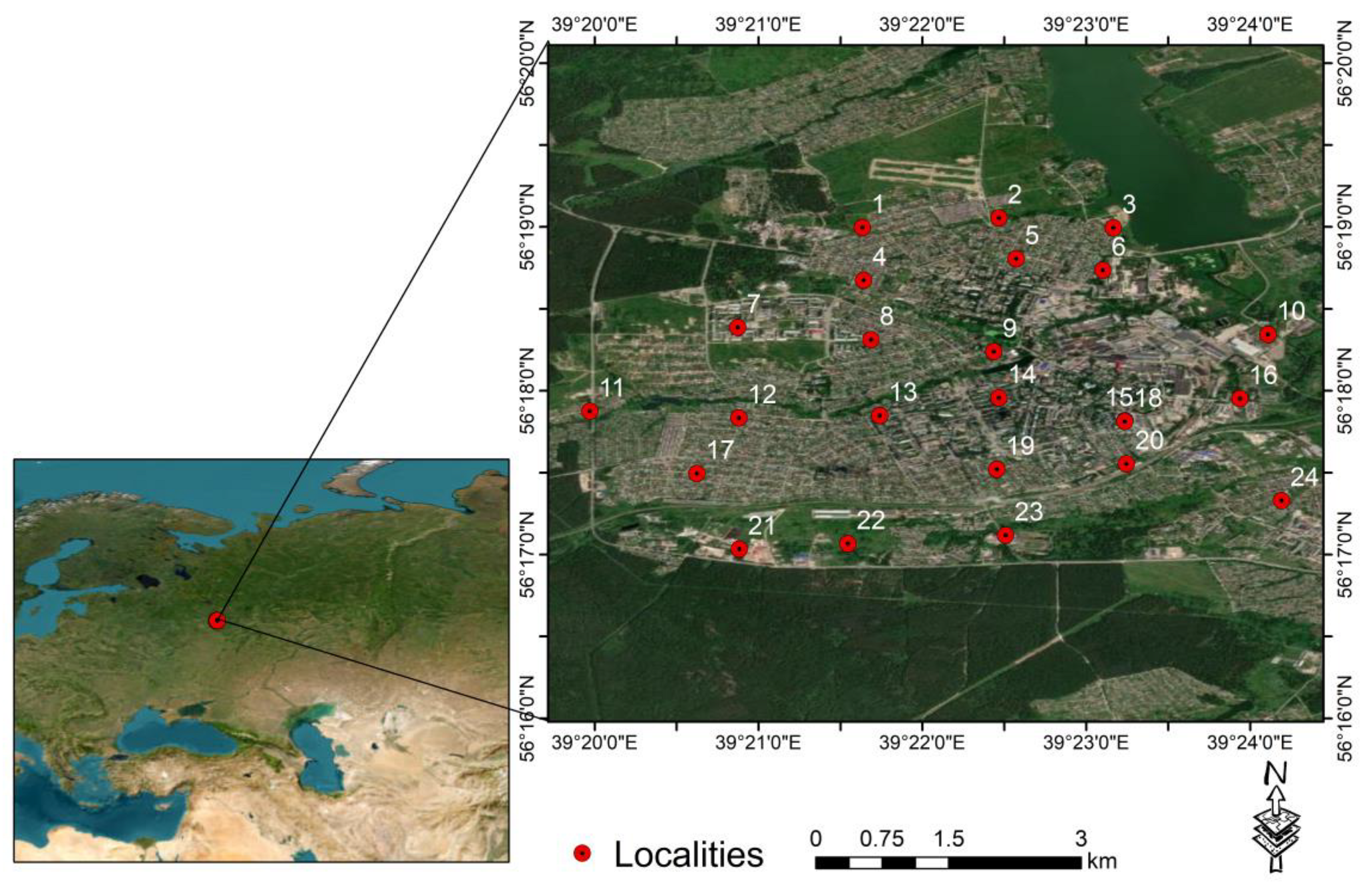
2.1. Sampling Strategy

A total of 24 soil samples were collected each of 1 kg from Kolchugino city, Vladimir Region–Russia. Kolchugino is located at 56°17′57″ N and 39°22′58″ E as shown in the map of localities as in Figure 1. It is characterized by Sod-podzolic soils (Dernovo-podzolistije (Sod-podzolic)) [20]. The samples were collected to cover the industrial pollution points. Therefore, the recommended sampling density was selected to be 1 sample per km2. In addition, a background sample was selected to compare the changes in soil quality in urban areas located at a distance of 5 km outside the city of Kolchugino. All the representative samples were collected by taking four samples 10 m apart at each individual site and mixed together. The samples were collected at 0–10 cm depth each. The samples were cleaned from roots and extraordinary things and transported to the laboratory for analysis. Prior to the analysis, the samples were dried till a constant weight, grinded, sieved, and homogenized.

2.2. Features of the Studied Area

The territory of the Kolchuginsky district belongs to the Central Russian province located in the center of the Russian Plain. Among the soils of the province, sod-podzolic predominates. The soil profile is more clearly differentiated by the eluvial-illuvial type. The soil cover is formed by combinations of sod-podzolic soils of different granulometric compositions and varying degrees of podzol with swamp-podzolic and swamp soils. Marsh-podzolic and marsh soils are confined mainly to lake-glacial and ancient alluvial low plains [21].
Two types are characterized by the soil cover: gray forest and sod-podzolic. Sod-podzolic are predominant. Alluvial soils are represented by other soils (in floodplains of rivers). Gray forest soils of different territories of the Kolchuginsky district differ significantly. On the elevated interfluves in the north, northeast and northwest, gray and light gray forest soils predominate [21].

2.3. Sample Preparation for Analysis

Soil samples were thoroughly mixed with a spatula and quantified. The samples were crushed by hand. The crushed soil was aligned on paper in the shape of a square, divided into four parts, two opposite parts were discarded, and the two remaining parts were mixed. The soil remaining after quartering was aligned on paper, conditionally divided into 6 squares, from the center of which approximately the same amount of soil was taken into a special envelope. The remaining amount of soil was grinded in a porcelain mortar with a wooden pestle and sieved with a diameter of 1 mm. The soil from a special envelope was sieved with a diameter of 0.25 mm.
The soil samples were weighted (1 g each) and then loaded into fluoroplastic reaction chambers. Aliquot of 5 mL of concentrated nitric acid (HNO3) and 0.5 mL of hydrogen peroxide (H2O2) were added. For carbonate soils—7 mL HNO3 and 0.5 mL H2O2 were added.
The reaction chambers were loaded into metal containers and tightly closed. Then, the metal containers were loaded into an autoclave and put to heat up to a temperature of 160 °C for 1 h. After an hour, the device is switched to a value of 180 °C, at this temperature, the hoods are heated for 2 h. Later on, the device is switched again, the temperature is raised to 200 °C and maintained in this mode for 1 h. The heating duration is counted from the moment when the selected temperature is reached (the deviation sensor on the device to show up 0).
After the heating of the hoods was completed, the containers were left to be cooled. After cooling in a special autoclave cooling unit, the containers are carefully opened (due to high internal pressure, the lid may be knocked out). Extracts are transferred quantitatively into measuring flasks (50 mL). The acid is drained, and the extract from the glasses is filtered into the flasks. After filtering, it is necessary to bring the extract to 50 mL of distilled water. The obtained extracts are further used to measure the content of heavy metals.

2.4. Analytical Method

The samples were analyzed at the ecological and analytical laboratory of the department of ecology and earth sciences of the university “Dubna”. The mass fraction of heavy metals was determined using QUANTUM-2A atomic absorption spectrometer (AAS) of NPO Cortec using atomization of the prepared sample in a flame (propane-butane mixture/air, with direct insertion of the sample into the flame). Gas-discharge lamps with a hollow cathode are used as radiation sources, spectral lines are isolated using a diffraction monochromator.
Calibration of the spectrometer was carried out using solutions of salts of the analyzed element prepared from standard samples of the composition. The selection and installation of optimal measurement conditions, as well as the processing of the results obtained, their archiving, storage and printing are carried out by the personal computer included in the device and specialized software.
The quality of the measurement was weighted and discussed (see Supplementary Materials).

2.5. Statistical Data Analysis

The statistical treatment of the results [22] was examined using the normal distribution of the elements’ mass fractions using the Shapiro–Wilk test [23]. All the relevant statistical analyses and infographics were carried out using The R Project for Statistical Computing [24]. The spatial distribution of the pollution patterns was studied using GIS technology and the data were interpolated using the inverse distance weighting (IDW) method.

3. Pollution Extent and Possible Webs

Two pollution indices have been computed to quantify the degree of contamination of soil elements. Pollution indices are effective tools for assessing the state of the environment and forecasting the ecosystem’s future pollution sustainability. The indices are the pollution load index (PLI) and total pollution index (TPI) [25,26]. In addition, the potential ecological and risk indices were calculated for the studied elements [27]. For the assessment of pollution level and associated risk, the background values were used as a baseline data.

3.1. The Pollution Load Index (PLI)

PLI demonstrates a good indicator of soil degradation due to heavy metal accumulation. PLI is calculated using the following equation [26,28].
PLI = i = 1 n P I i n
where n denotes the number of metals and PI denotes the single pollution index, which is defined as the concentration of each element divided by its abundance in continental shale [29]. When (PLI) is more than one, pollution is present. Otherwise, there is no pollution.

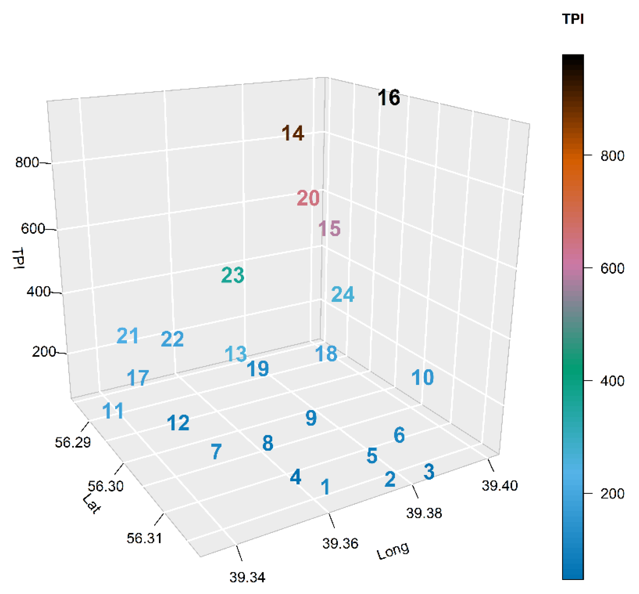
3.2. Total Pollution Index TPI (Zc)

The level of chemical contamination of soil is estimated as an indicator of negative impact on public health using indicators developed in complex geochemical studies. Similar to PLI, TPI is calculated by comparing the chemical concentration of element Ci (mg/kg) with the regional background Cbi. Since the study takes into account the background, the corresponding value of the same element in the background was used to determine the amount of contamination [29,30]. The chemical mass fractions’ coefficient is expressed in Kc and given as:
K c = C i / C b i  
The summation of Kc is TPI and given as:
T P I = i = 1 n K c i n 1  
where n stands for the number of the elements and Kci is the concentration coefficient higher than 1 of i element [30,31,32].

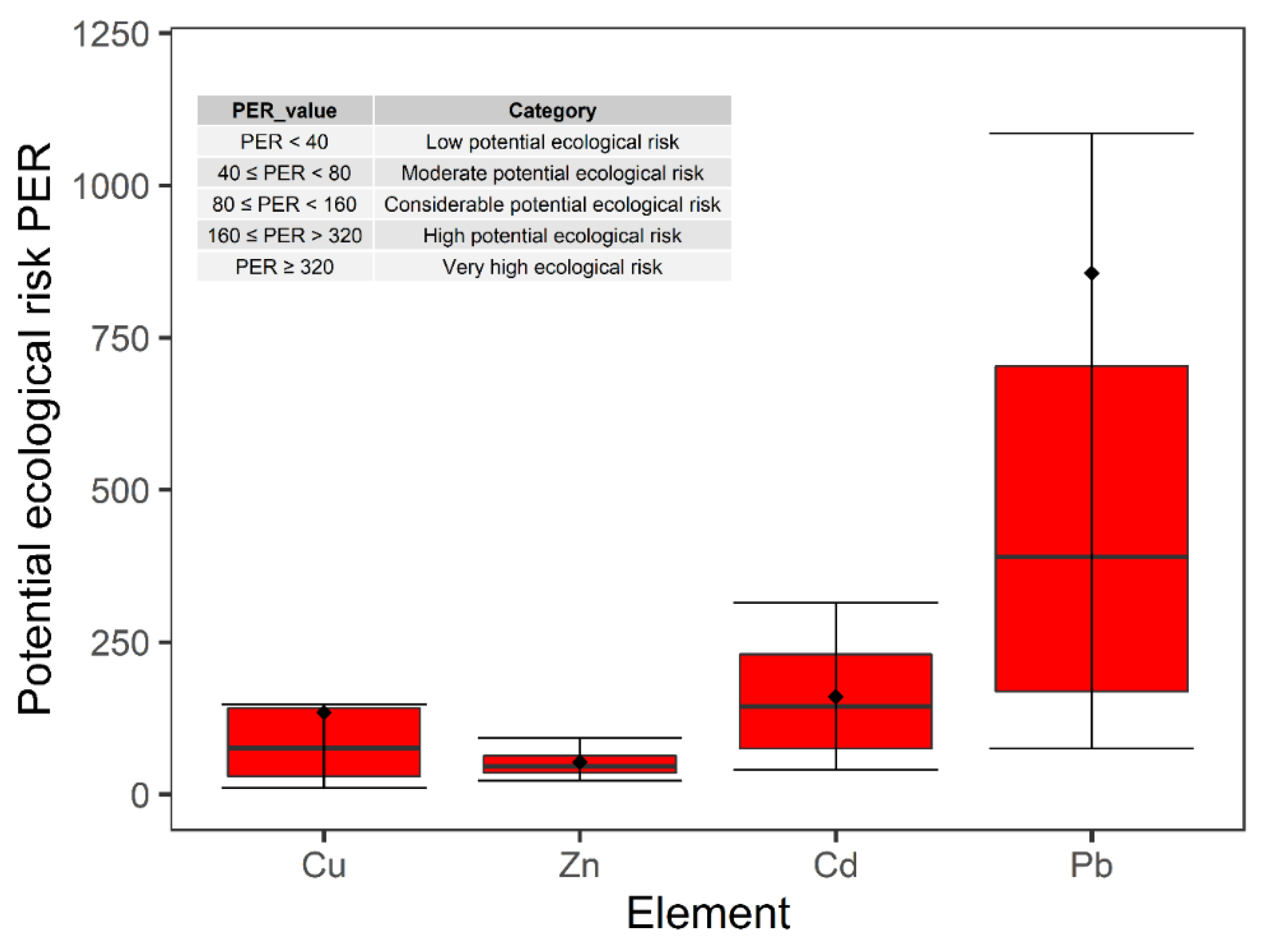
3.3. Potential Ecological Risk Index (PER)

PER is a diagnostic tool for controlling soil pollution and classifying areas that should be given special attention [27]. The formula of P E R f i for single metal pollution is
P E R f i = C f i × T f i
where P E R f i is the potential ecological risk index, C f i is the contamination factor, and T f i is the “toxic-response” coefficient for single metal. The corresponding T f i values are Zn = 1, Pb = Cu = 5, and Cd = 30 [6,27].

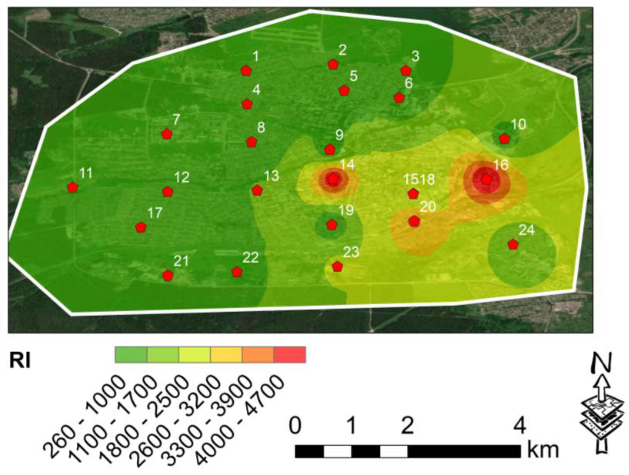
3.4. Risk Index (RI)

RI is an index that joins all of the metals, is given as
R I = P E R f i
where (RI) is the sum of P E R f i for each metal of interest [27]. The interpretation categories for PER are given as an inset in Figure 7. Additionally, RI is given in the Supplementary Materials.

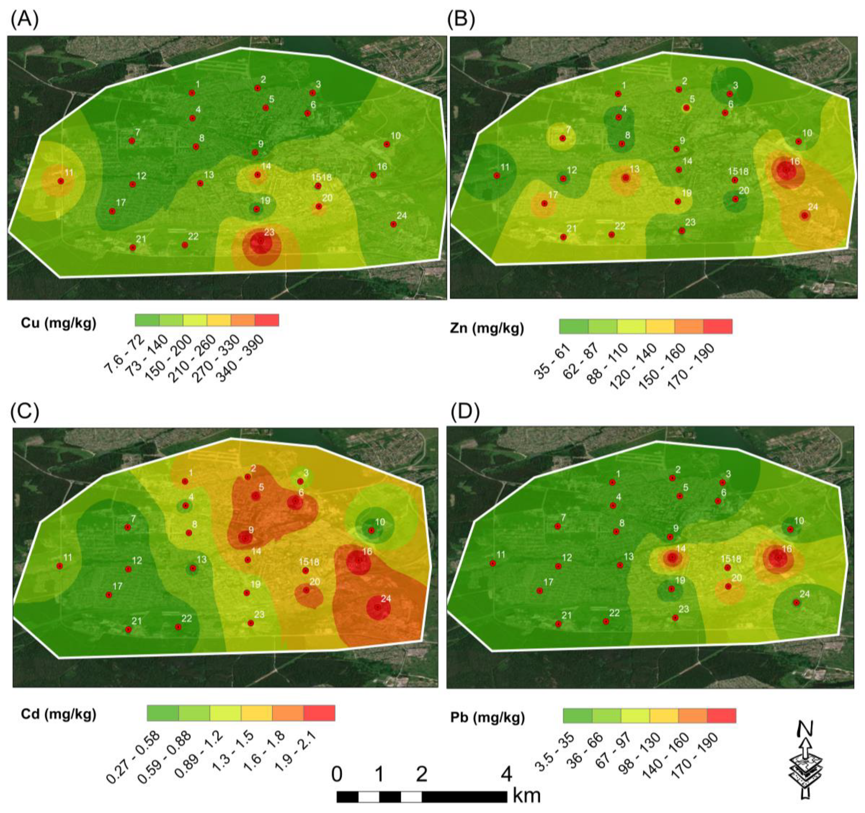
4. Remote Sensing Data and Analysis

Remote sensing images were used to disengage the different land-use land-cover (LULC) in the study area. An Operational Land Imager (OLI), was used which acquired data on 31 July 2021 with 30 m spatial resolution. The maximum likelihood method was applied to classify the satellite images to get LULC map. The reprocessing (radiometric and atmospheric calibration) of satellite images was achieved using ENVI (Exelis Visual Information Solutions, Boulder, CO, USA) software 5.3 (Lillesand et al., 2000). A detailed description of the methodology and its utilization has been widely reported and published elsewhere by Mohamed, et al. [33], Mohamed, et al. [34], Abdel-Fattah, et al. [35].

5. Results and Discussion

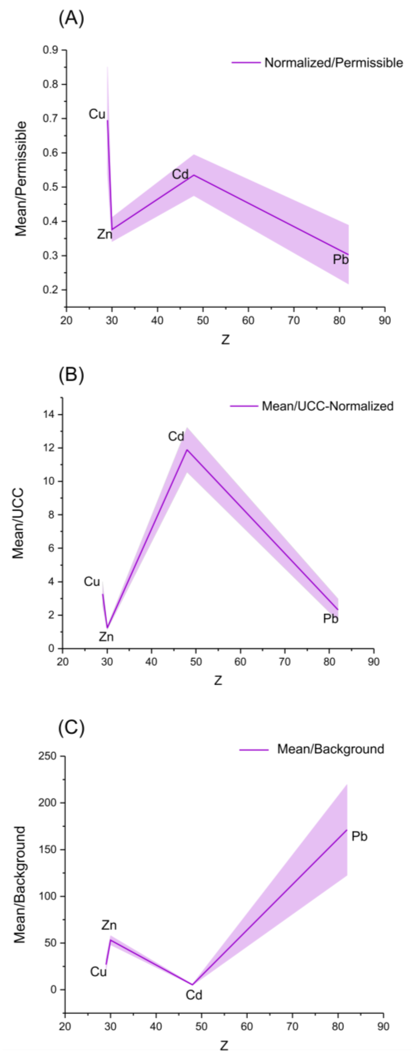
5.1. Elemental Abundances

The descriptive statistics of 24 sod podzolic samples is given in Table 1. The table shows the mass fractions in mg/kg for the studied toxic elements (Cu, Zn, Cd, and Pb). The mean and standard error of Cu were found to be 92 ± 21 mg/kg, with a range of 8 to 391 mg/kg for locations #12 and 23, respectively. Similarly, the average ± se value of Zn was determined to be 83 ± 8 mg/kg, ranging from 35 to 190 mg/kg for locations #11 and 16, respectively. Likewise, the mass fraction of Cd was determined to be 1 ± 0.1 mg/kg, with a range of 0.3 to 2 mg/kg, for locations 7 and 16. Finally, the mass fraction of Pb is calculated to be 39 ± 11 mg/kg, with a range of 3 to 190 mg/kg for locations 3 and 16, respectively. It is obvious that location 16 poses significant amounts of the studied toxic elements. This peculiarity can be explained by the existence of a powerful industrial infrastructure in the investigated city, As the basis of the city’s economy is industrial production, for example mechanical engineering, metalworking, non-ferrous metallurgy, and electric power industry. Therefore, there is a various number of pollution sources in the area under investigation. In addition, the basic descriptive statistical analysis was summarized and provided in Table 2. For comparison purposes, the obtained results were compared by Rudnick and Gao [36] for UCC and Vinogradov [37] for soil. The comparison shows that the obtained results are much higher than those from the literature, which in turn, may pose a significant hazard to humans and the environment.
The mean and median values are quite different except for Cd, and it could be hypothesized that the obtained results of the mass fractions are not normally distributed. The normality test was carried out using the Shapiro–Wilk test [23], with a 95% probability (p ≤ 0.05). The results of the normality test show that the elements are not normally distributed except Cd (p = 0.075). The obtained mass fractions of the toxic elements in soil samples show remarkable variations with a range from a minimum value of 46% for Zn to a maximum value of 139% for Pb with a mean ± sd values of CV% of 88 ± 44. Referring to the fact that high values of CV (>75%), positive skewness (>0), and kurtosis (>3) mostly indicate the non-normal distribution of the mass fractions [38,39,40].
The mass fractions in mg/kg for the determined elements were interpolated and mapped using ArcGIS as clearly shown in Figure 2.
The mass fraction of Cu was mapped to be in considerable amounts in location 23. This finding can be explained by the existence of anthropogenic activities as in Figure 2A.
The map of the spatial distribution of Zn, Figure 2B shows that the peak value was noticed for locations 16 and a little for location 24. Most probably because of the association of the non-ferrous metallurgy plants.
Locations 5, 9, 6, 20, 24, show a high amount of Cd as in Figure 2C. However, location 16 shows the highest contribution and is most likely because of the same pollution source,
Likewise, Figure 2D shows that the mass fractions of Pb are remarkable in locations 14 and 16.
Eventually, the significant contribution of PTMs comes mainly from the same locations 16 and 14, except Cu comes from locations 23.
As a summing up, location 16 has a considerable contribution to the elevated amounts of the mass fractions of the studied elements. Most likely, it comes from the plant of non-ferrous metallurgy.
The results were normalized to three normalizers to eliminate the influence of background element concentrations and to see how far they differed from the corresponding permissible concentration values, the upper continental crust UCC of Rudnick and Gao [36] and the background concentration determined from a representative sample from a clean and undisturbed soil profile. The concept of “background” is quite subjective in terms of the case study and has been discussed in detail by many researchers [38,40,41]. To distinguish between geogenic and anthropogenic influences of elevated mass fractions of determining elements, three approaches were followed on a regional basis using a sample representative of the background, and on a global basis using the corresponding UCC values for normalization [36].
The results of the normalization are plotted and illustrated in Figure 3. The figure of normalization of the elements to the permissible concentrations depicts that there is no considerable pollution and the elements do not pose any hazardous impact to the environment as clearly shown in Figure 3A, whereas the illustrations of the normalization to the corresponding values of UCC and background in Figure 3B,C, respectively shows that there are considerable amounts of toxic elements accumulated in the soil samples of the investigated city. Specifically, the normalization of the mass fractions of the elements to the background values shows rather high pollution in the studied samples, which may lead to adverse effects on public health impacts.
In summary, the first and third approaches seem to underestimate and overestimate, respectively, the ecological situation in terms of pollution. Despite the fact that the second approach is more appropriate, in the present work the regional background has been used for subsequent calculations in order to avoid potential threats to the environment and individuals. Thus, the obtained results can serve as good baseline data that can help decision-makers to get rid of this problem, control the disposal of industrial waste and set limits based on a reliable scientific result that can be only acquired by data accumulation and analysis.

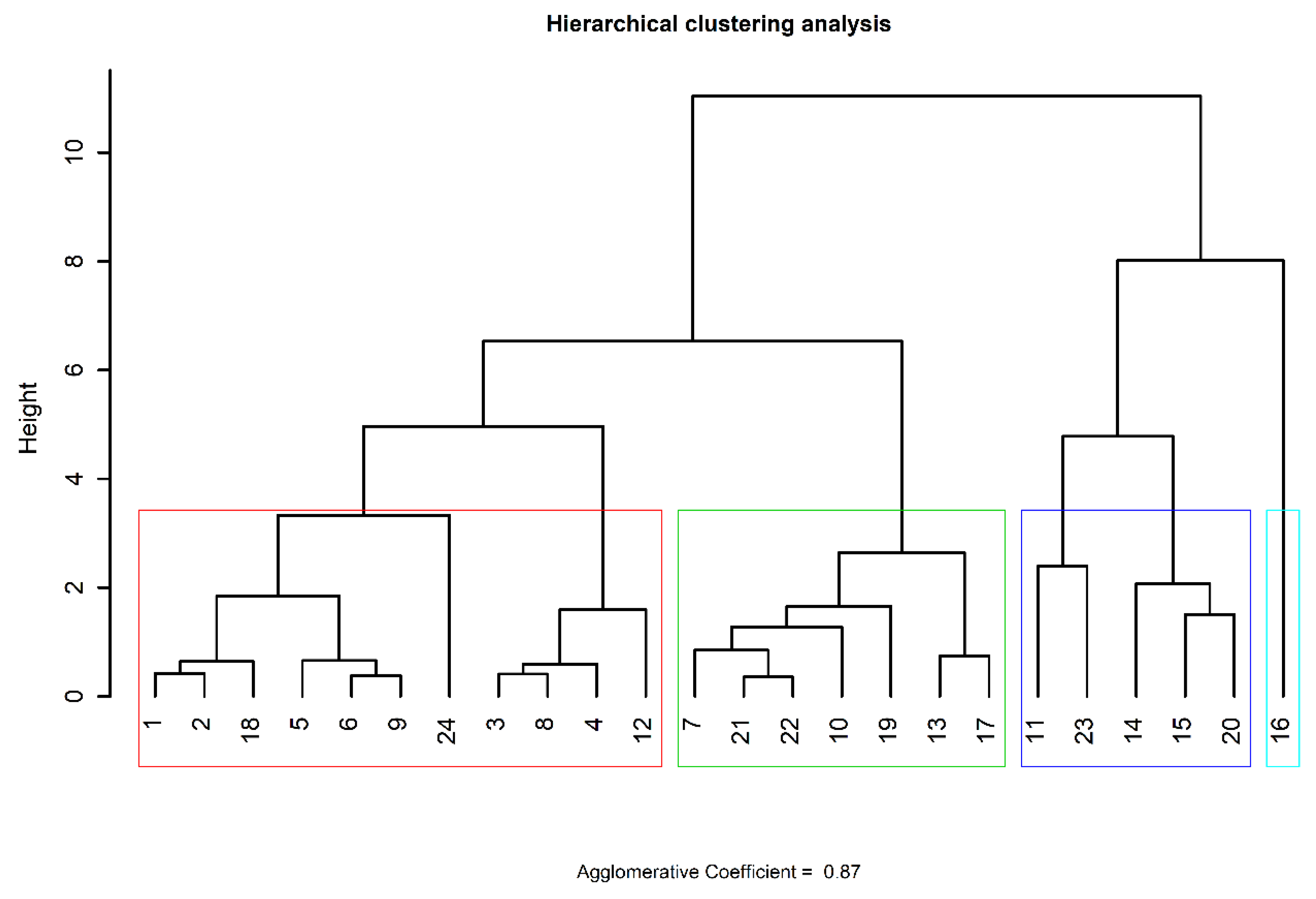
5.2. Hierarchical Clustering Analysis (HCA)

HCA distinguishes itself by offering a broader selection of distance metrics and grouping techniques [42]. HCA was proceeded based on the geochemical data of the determining elements [24]. Specifically, the package “cluster” for agglomerative nesting AGNES was used. Agglomerative hierarchical clustering is the most common type of hierarchical clustering, where observations are linked into groups based on their similarity or dissimilarity. More details about the various functions and applications are published by [43,44]. To extract information on the appropriate metric of similarity matrix reproduction and the proper method of clustering, the most well-known methods for clustering were computed in terms of agglomerative coefficient and the larger the coefficient, the better the method fits the dataset the dataset. Therefore, the Euclidean metric for the creation of similarity/dissimilarity matrix and the ward method for clustering were implemented. The agglomerative coefficients (AC) of different methods were 0.80, 0.75, 0.83, 0.88, and 0.79 for average, single, complete, Ward, and weighted, respectively. Based on the calculated AC, the highest one was noticed for the ward method of clustering. Based on the extracted information about the metric and method of clustering, the agglomerative hierarchical clustering was plotted and illustrated in Figure 4. The figure depicts four groups of locations that are joined based on their similar geochemical data. The four groups can be discussed as:
The first cluster contains 11 locations, namely 1, 2, 18, 5, 6, 9, 24, 3, 8, 4, and 12. In fact, there are almost four subclusters and it seems that location 24 contains a separate one. Most probably, it has different geochemical data over the others and that is why it contains a separate subcluster. Location 24 is characterized by metallurgical plants.
The second cluster includes locations 7, 21, 22, 10, 19, 13, and 17.
The third group has 5 locations, namely 11, 23, 14, 15, and 20. Locations 14 and 20 are characterized by common geochemical traits. Mostly, they share the same sources of pollution.
Location 16 tended to make a separate group and this peculiarity can be explained by the existence of the factories and metallurgical plants which can be considered the main pollution source in the town.

6. Remarks on the Pollution Extent

The pollution by the toxic elements in the soils of Kolchugino city, Vladimir Region has been assessed using different pollution indices. As mentioned above, before the calculation of the PLI and TPI, the single pollution index for every single element was computed and later on the assessment of PLI and TPI was carried out. In the present work, the same approach of PI and Kc calculation is the same. They have been calculated by dividing the mass fraction of element i by the corresponding value of the same element in the background [3,5,6,45]. The average mass fractions ± standard error of the obtained results for Kc are 5.4 ± 0.6 with a minimum value of 1.4 and a maximum value of 10.5 were noticed for locations 7 and 16 for Cd; 26.9 ± 6.0 and a range of 2.2 to 114.7 were noticed for locations 12 and 23 for Cu; 171.2 ± 48.6 and a range from 15.1 to 828.2 were noticed for locations 3 and 16 for Pb; and finally, 53.1 ± 5.0 and a range from 22.5 to 121.8 were noticed for locations 11 and 16 for Zn, respectively. It is apparent from the obtained results of PI and Kc that a remarkable contribution of pollution is linked to location 16. The ranked geochemical spectrum of the toxic elements is as follows; Cd5.4, Cu26.9, Zn53.1, and Pb171.2.
Based on the obtained results of the single pollution index, the pollution load PLI and total pollution indices TPI were calculated. The average value ± standard error of PLI is found to be 256.5 ± 53.6 with a minimum value of 49.6 to a maximum value of 982.2, were noticed for locations 24 and 1, respectively. While for TPI the average value ± se is found to be 253.5 ± 53.6 with a minimum value of 46.6 to a maximum value of 979.2, were noticed for locations 24 and 1, respectively. The results of PLI are mapped and illustrated Figure 5. The results of TPI are illustrated on Figure 6. Based on the interpretation criteria of PLI and TPI, the figures show a good consistency, and depict that location 16 has a significant contribution to the increased pollution in the area under investigation.
PER was calculated based on the studied elements and the results were illustrated and shown in Figure 7. PER was noticed to be significant and the highest value was recorded for Pb and in turn, it is classified as high ecological risk according to the inset table of the interpretation. The risk index (RI) is the summation of PER for each single element. The spatial distribution of RI is mapped Figure 8. The figure depicts the peak values were noticed for locations 14 and 16. In fact, according to their interpretation and classes [6,27,46], all the pollution indices studied have identified the same places as top areas and should be considered with great attention in order to decrease the level of pollution by regulating the waste disposal of factories and enterprises.

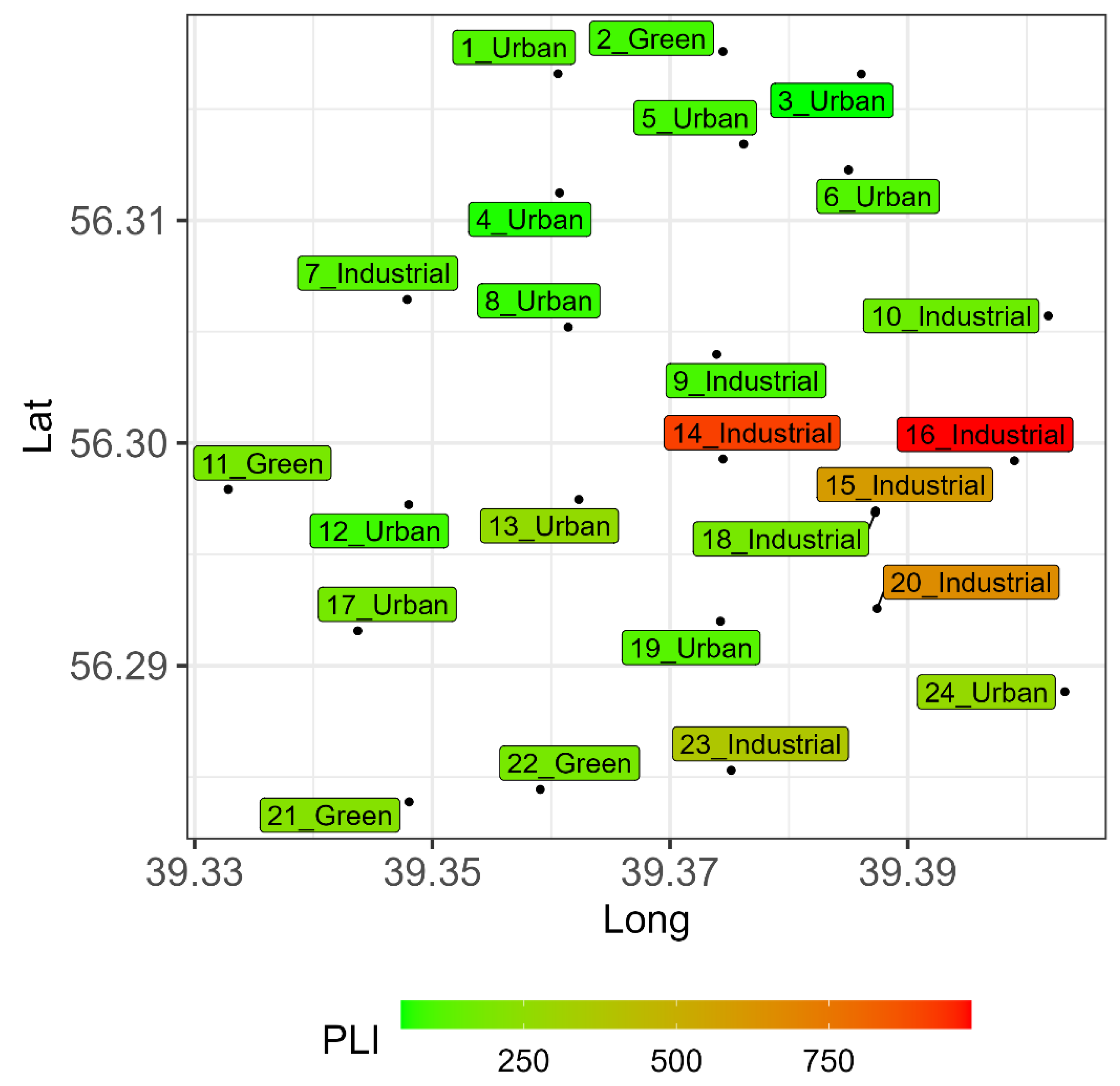
7. Observations of Land-Use/Land-Cover (LCLU)

The maximum likelihood was applied to Operational Land Imager (OLI) to classify the land-use land-cover map. The results revealed six types of land-use/land-cover, namely urban, water, green, forest, swamps, and industrial areas. The results of the land-use land-cover are illustrated and mapped as shown in Figure 9. Furthermore, the map shows that the urban type is dominant. The results of the identification are quite consistent and demonstrate a good agreement with the above discussed observations of the pollution sources. The industrial areas are directly linked to the existence of the ferrous factories and correspond to the locations of the highest association of pollution.
The findings of LULC were linked with the pollution load index (PLI). Comparing the outcomes of (LULC) and (PLI), it was found that the maximum value of (PLI) is 982 and the minimum value is 49.6 for locations 16 (industrial area) and 3 (urban area), respectively. Although there are areas were classified as urban areas, their (PLI) was also significant. These peculiarities can be explained by the fact that these locations are adjacent to the industrial areas and mostly were affected due to the weathering. For instance, locations 24 and 13. The results of the calculated (PLI) and their corresponding areas are plotted and illustrated in Figure 10. Furthermore, detailed information on the pollution indices and the corresponding locations and areas analyzed by LULC is provided in Table 2 (Supplementary Materials).

8. Conclusions

The present work achieves its primary objectives by providing a comprehensive characterization of the four toxic elements Cu, Zn, Cd, and Pb and their associated pollution in soil samples. The data normalized with the three different normalizers have shown that it is appropriate to normalize the data in accordance with the corresponding regional or local values to avoid over- or underestimation of the data. The study identified sites with significant mass fractions, such as location 23 for Cu, location 16 for Zn, locations 5, 6, 9, 16, 20, 24 for Cd, and finally, locations 14 and 16 for Pb. Locations 14 and 16 were classified as polluted areas based on the analyzed results of pollution indices. The LULC shows that the urban class is the dominant one among six classes revealed from the results. The locations of peak spots of pollution were identified as industrial areas and are quite comparable with the obtained results of pollution indices. The obtained data can serve as scientific evidence for the pollution of the industrial city with toxic elements and great attention should be paid to eliminating the pollution sources and regulating waste disposal.

Supplementary Materials

The following supporting information can be downloaded at: https://www.mdpi.com/article/10.3390/land12020439/s1, Figure S1: title; Table S1: the standard mass fraction of the standard and the measured (mg/kg); Table S2: details on the pollution indices and the corresponding areas analyzed by LULC.

Author Contributions

Conceptualization, W.M.B. and I.Z.K.; methodology, S.P.K.; software, W.M.B.; validation, W.M.B., I.Z.K. and S.P.K.; formal analysis, W.M.B.; investigation, I.Z.K.; resources, I.Z.K.; data curation, W.M.B., O.A.M. and S.V.M.; writing—original draft preparation, W.M.B.; writing—review and editing, W.M.B., S.V.M. and O.A.M.; visualization, W.M.B.; supervision, I.Z.K. and W.M.B. All authors have read and agreed to the published version of the manuscript.

Funding

This research received no external funding.

Data Availability Statement

The data are provided in this study.

Conflicts of Interest

The authors declare no conflict of interest.

References

  1. El Behairy, R.A.; El Baroudy, A.A.; Ibrahim, M.M.; Mohamed, E.S.; Rebouh, N.Y.; Shokr, M.S. Combination of GIS and Multivariate Analysis to Assess the Soil Heavy Metal Contamination in Some Arid Zones. Agronomy 2022, 12, 2871. [Google Scholar] [CrossRef]
  2. El-Taher, A.; Badawy, W.M.; Alshahrani, B.; Ibraheem, A.A. Neutron activation and ICP-MS analyses of metals in dust samples-Kingdom of Saudi Arabia: Concentrations, pollution, and exposure. Arab. J. Geosci. 2019, 12, 635. [Google Scholar] [CrossRef]
  3. Badawy, W.M.; Sarhan, Y.; Duliu, O.G.; Kim, J.; Yushin, N.; Samman, H.E.; Hussein, A.A.; Frontasyeva, M.; Shcheglov, A. Monitoring of air pollutants using plants and co-located soil-Egypt: Characteristics, pollution, and toxicity impact. Environ. Sci. Pollut. Res. Int. 2022, 29, 21049–21066. [Google Scholar] [CrossRef]
  4. Madadzada, A.I.; Badawy, W.M.; Hajiyeva, S.R.; Veliyeva, Z.T.; Hajiyev, D.B.; Shvetsova, M.S.; Frontasyeva, M.V. Assessment of atmospheric deposition of major and trace elements using neutron activation analysis and GIS technology: Baku-Azerbaijan. Microchem. J. 2019, 147, 605–614. [Google Scholar] [CrossRef]
  5. Badawy, W.M.; Duliu, O.G.; Frontasyeva, M.V.; El-Samman, H.; Mamikhin, S.V. Dataset of elemental compositions and pollution indices of soil and sediments: Nile River and delta-Egypt. Data Brief 2020, 28, 105009. [Google Scholar] [CrossRef]
  6. Badawy, W.M.; El-Taher, A.; Frontasyeva, M.V.; Madkour, H.A.; Khater, A.E.M. Assessment of anthropogenic and geogenic impacts on marine sediments along the coastal areas of Egyptian Red Sea. Appl. Radiat. Isot. 2018, 140, 314–326. [Google Scholar] [CrossRef]
  7. Morton-Bermea, O.; Hernández-Álvarez, E.; González-Hernández, G.; Romero, F.; Lozano, R.; Beramendi-Orosco, L.E. Assessment of heavy metal pollution in urban topsoils from the metropolitan area of Mexico City. J. Geochem. Explor. 2009, 101, 218–224. [Google Scholar] [CrossRef]
  8. Tong, S.; Li, H.; Wang, L.; Tudi, M.; Yang, L. Concentration, Spatial Distribution, Contamination Degree and Human Health Risk Assessment of Heavy Metals in Urban Soils across China between 2003 and 2019-A Systematic Review. Int. J. Environ. Res. Public Health 2020, 17, 3099. [Google Scholar] [CrossRef]
  9. Shokr, M.S.; Abdellatif, M.A.; El Behairy, R.A.; Abdelhameed, H.H.; El Baroudy, A.A.; Mohamed, E.S.; Rebouh, N.Y.; Ding, Z.; Abuzaid, A.S. Assessment of Potential Heavy Metal Contamination Hazards Based on GIS and Multivariate Analysis in Some Mediterranean Zones. Agronomy 2022, 12, 3220. [Google Scholar]
  10. Hammam, A.A.; Mohamed, W.S.; Sayed, S.E.-E.; Kucher, D.E.; Mohamed, E.S. Assessment of Soil Contamination Using GIS and Multi-Variate Analysis: A Case Study in El-Minia Governorate, Egypt. Agronomy 2022, 12, 1197. [Google Scholar] [CrossRef]
  11. Abuzaid, A.S.; Jahin, H.S.; Shokr, M.S.; El Baroudy, A.A.; Mohamed, E.S.; Rebouh, N.Y.; Bassouny, M.A. A Novel Regional-Scale Assessment of Soil Metal Pollution in Arid Agroecosystems. Agronomy 2023, 13, 161. [Google Scholar] [CrossRef]
  12. Abdusamadzoda, D.; Abdushukurov, D.A.; Duliu, O.G.; Zinicovscaia, I. Assessment of the Toxic Metals Pollution of Soil and Sediment in Zarafshon Valley, Northwest Tajikistan (Part II). Toxics 2020, 8, 113. [Google Scholar] [CrossRef]
  13. Abu-hashim, M.; Lilienthal, H.; Schnug, E.; Kucher, D.E.; Mohamed, E.S. Tempo-Spatial Variations in Soil Hydraulic Properties under Long-Term Organic Farming. Land 2022, 11, 1655. [Google Scholar] [CrossRef]
  14. Abdel-Fattah, M.K.; Mohamed, E.S.; Wagdi, E.M.; Shahin, S.A.; Aldosari, A.A.; Lasaponara, R.; Alnaimy, M.A. Quantitative evaluation of soil quality using Principal Component Analysis: The case study of El-Fayoum depression Egypt. Sustainability 2021, 13, 1824. [Google Scholar] [CrossRef]
  15. Cai, J.S.; Chen, S.Y.; Yu, G.Q.; Zou, Y.F.; Lu, H.X.; Wei, Y.; Tang, J.X.; Long, B.S.; Tang, X.; Yu, D.M.; et al. Comparations of major and trace elements in soil, water and residents? hair between longevity and non-longevity areas in Bama, China. Int. J. Environ. Health Res. 2021, 31, 581–594. [Google Scholar] [CrossRef]
  16. Mohamed, E.; Ali, A.; El Shirbeny, M.; Abd El Razek, A.A.; Savin, I.Y. Near infrared spectroscopy techniques for soil contamination assessment in the Nile Delta. Eurasian Soil Sci. 2016, 49, 632–639. [Google Scholar] [CrossRef]
  17. Li, Y.; Liu, F.; Zhou, X.; Wang, X.; Liu, Q.; Zhu, P.; Zhang, L.; Sun, C. Distribution and Ecological Risk Assessment of Heavy Metals in Sediments in Chinese Collapsed Lakes. Pol. J. Environ. Stud. 2017, 26, 181–188. [Google Scholar] [CrossRef]
  18. Mohamed, E.S.; Baroudy, A.A.E.; El-beshbeshy, T.; Emam, M.; Belal, A.; Elfadaly, A.; Aldosari, A.A.; Ali, A.M.; Lasaponara, R. Vis-nir spectroscopy and satellite landsat-8 oli data to map soil nutrients in arid conditions: A case study of the northwest coast of egypt. Remote Sens. 2020, 12, 3716. [Google Scholar]
  19. Bityukova, V.R. Environmental Problems of Small Towns in Russia. In Bulletin of Moscow University Geography; Geography and Ecology; Moscow University: Moscow, Russia, 2007; Volume 1. [Google Scholar]
  20. IUSS Working Group WRB. World Reference Base for Soil Resources 2014, Update 2015 International Soil Classification System for Naming Soils and Creating Legends for Soil Maps; World Soil Resources Reports No. 106; FAO: Rome, Italy, 2015. [Google Scholar]
  21. The Information System of the Soil-Geographical Database of Russia. Soil of Russia. Available online: https://soil-db.ru/map?lat=56.1149&lng=39.8941&zoom=9 (accessed on 8 February 2022).
  22. Reimann, C.; Filzmoser, P. Normal and lognormal data distribution in geochemistry: Death of a myth. Consequences for the statistical treatment of geochemical and environmental data. Environ. Geol. 2000, 39, 1001–1014. [Google Scholar] [CrossRef]
  23. Shapiro, S.S.; Wilk, M.B. An analysis of variance test for normality (complete samples). Biometrika 1965, 52, 591–611. [Google Scholar] [CrossRef]
  24. R Core Team R: A Language and Environment for Statistical Computing; R Foundation for Statistical Computing: Vienna, Austria, 2020. Available online: https://www.R-project.org/ (accessed on 8 February 2022).
  25. Kowalska, J.; Mazurek, R.; Gąsiorek, M.; Setlak, M.; Zaleski, T.; Waroszewski, J. Soil pollution indices conditioned by medieval metallurgical activity—A case study from Krakow (Poland). Environ. Pollut. 2016, 218, 1023–1036. [Google Scholar] [CrossRef]
  26. Kowalska, J.B.; Mazurek, R.; Gąsiorek, M.; Zaleski, T. Pollution indices as useful tools for the comprehensive evaluation of the degree of soil contamination—A review. Environ. Geochem. Health 2018, 40, 2395–2420. [Google Scholar] [CrossRef] [Green Version]
  27. Hakanson, L. An ecological risk index for aquatic pollution control.a sedimentological approach. Water Res. 1980, 14, 975–1001. [Google Scholar] [CrossRef]
  28. Varol, M. Assessment of heavy metal contamination in sediments of the Tigris River (Turkey) using pollution indices and multivariate statistical techniques. J. Hazard. Mater. 2011, 195, 355–364. [Google Scholar] [CrossRef]
  29. Li, Y.H.; Schoonmaker, J.E. 9.1—Chemical Composition and Mineralogy of Marine Sediments. In Treatise on Geochemistry, 2nd ed.; Holland, H.D., Turekian, K.K., Eds.; Elsevier: Oxford, UK, 2014; pp. 1–32. [Google Scholar]
  30. Saet, Y.E.; Revich, B.A.; Yanin, E.P.; Smirnova, R.S.; Basharkevich, I.L.; Onishchenko, T.L.; Pavlova, L.N.; Trefilova, N.Y.; Achkasov, A.I.; Sarkisyan, S.S. Geochemistry of the Environment; NEDRA: Waltham, MA, USA, 1990. [Google Scholar]
  31. Andreev, D.N.; Dzyuba, E.A. Total soil heavy metal contamination in various biotops at the territory of Vishersky reserve. Gen. Biol. 2016, 64, 5. [Google Scholar]
  32. Shaykhutdinova, A.N. Assessment of the degree of contamination agricultural soils Kuzbass mobile forms of heavy metals. In Proceedings of the V International Scientific Conference Dedicated to the 85th Anniversary of the Department of Soil Science and Soil Ecology of TSU, Tomosk, Russia, 10 August 2015; p. 5. [Google Scholar]
  33. Mohamed, E.S.; Ali, A.; El-Shirbeny, M.; Abutaleb, K.; Shaddad, S.M. Mapping soil moisture and their correlation with crop pattern using remotely sensed data in arid region. Egypt. J. Remote Sens. Space Sci. 2020, 23, 347–353. [Google Scholar] [CrossRef]
  34. Mohamed, E.S.; Abu-hashim, M.; AbdelRahman, M.A.E.; Schütt, B.; Lasaponara, R. Evaluating the Effects of Human Activity over the Last Decades on the Soil Organic Carbon Pool Using Satellite Imagery and GIS Techniques in the Nile Delta Area, Egypt. Sustainability 2019, 11, 2644. [Google Scholar] [CrossRef]
  35. Abdel-Fattah, M.K.; Abd-Elmabod, S.K.; Aldosari, A.A.; Elrys, A.S.; Mohamed, E.S. Multivariate Analysis for Assessing Irrigation Water Quality: A Case Study of the Bahr Mouise Canal, Eastern Nile Delta. Water 2020, 12, 2537. [Google Scholar]
  36. Rudnick, R.L.; Gao, S. Composition of the Continental Crust. In Treatise on Geochemistry; Turekian, K.K., Ed.; Elsevier: Oxford, UK, 2014; pp. 1–51. [Google Scholar]
  37. Vinogradov, A.P. The Geochemistry of Rare and Dispersed Chemical Elements in Soils, 2nd ed.; Consultants Bureau Enterprises: New York, NY, USA, 1959. [Google Scholar]
  38. Allajbeu, S.; Yushin, N.S.; Qarri, F.; Duliu, O.G.; Lazo, P.; Frontasyeva, M.V. Atmospheric deposition of rare earth elements in Albania studied by the moss biomonitoring technique, neutron activation analysis and GIS technology. Environ. Sci. Pollut. Res. 2016, 23, 14087–14101. [Google Scholar] [CrossRef]
  39. Hair, J.F.; Sarstedt, M.; Pieper, T.M.; Ringle, C.M. The use of partial least squares structural equation modeling in strategic management research: A review of past practices and recommendations for future applications. Long Range Plan. 2012, 45, 320–340. [Google Scholar] [CrossRef]
  40. Zhou, X.; Chen, Q.; Liu, C.; Fang, Y. Using moss to assess airborne heavy metal pollution in Taizhou, China. Int. J. Environ. Res. Public Health 2017, 14, 430. [Google Scholar] [CrossRef]
  41. Chaligava, O.; Shetekauri, S.; Badawy, W.M.; Frontasyeva, M.V.; Zinicovscaia, I.; Shetekauri, T.; Kvlividze, A.; Vergel, K.; Yushin, N. Characterization of Trace Elements in Atmospheric Deposition Studied by Moss Biomonitoring in Georgia. Arch. Environ. Contam. Toxicol. 2021, 80, 350–367. [Google Scholar] [CrossRef]
  42. Carlson, D.L. Quantitative Methods in Archaeology Using R; University of Cambridge: Cambridge, UK, 2017. [Google Scholar]
  43. Struyf, A.; Hubert, M.; Rousseeuw, P. Clustering in an Object-Oriented Environment. J. Stat. Softw. 1997, 1, 1–30. [Google Scholar] [CrossRef]
  44. Kaufman, L.; Rousseeuw, P.J. Agglomerative Nesting (Program AGNES). In Finding Groups in Data; John Wiley & Sons: Hoboken, NJ, USA, 1990; pp. 199–252. [Google Scholar]
  45. Badawy, W.; Chepurchenko, O.Y.; El Samman, H.; Frontasyeva, M.V. Assessment of Industrial Contamination of Agricultural Soil Adjacent to Sadat City, Egypt. Ecol. Chem. Eng. S-Chem. I Inz. Ekol. S 2016, 23, 297–310. [Google Scholar] [CrossRef] [Green Version]
  46. Karuppasamy, M.P.; Qurban, M.A.; Krishnakumar, P.K.; Mushir, S.A.; Abuzaid, N. Evaluation of toxic elements As, Cd, Cr, Cu, Ni, Pb and Zn in the surficial sediments of the Red Sea (Saudi Arabia). Mar. Pollut. Bull. 2017, 119, 181–190. [Google Scholar] [CrossRef]
Figure 1. Map of samples’ locations.
Land 12 00439 g001
Figure 2. The spatial distribution of the mass fractions (mg/kg) for Cu, Z, Cd, and Pb from (AD), respectively.
Land 12 00439 g002
Figure 3. Spidergram shows the normalized mass fractions to various normalizers; the permissible values (A), to the upper continental crust UCC (B), and background (C) values.
Land 12 00439 g003
Figure 4. Agglomerative clustering analysis of the studied locations.
Land 12 00439 g004
Figure 5. The spatial distribution of PLI in the studied city.
Land 12 00439 g005
Figure 6. The distribution of the total pollution index (TPI).
Land 12 00439 g006
Figure 7. PER and the corresponding range for each category.
Land 12 00439 g007
Figure 8. The distribution of risk index illustrating locations with significant values.
Land 12 00439 g008
Figure 9. Distribution of land-use/land-cover map illustrating six classes.
Land 12 00439 g009
Figure 10. The distribution of PLI and the corresponding areas obtained by LULC.
Land 12 00439 g010
Table 1. The mass fractions mg/kg of the obtained elements and the corresponding locations.
IDLatLongCuZnCdPb
156.316639.360629.7 ± 1.271.4 ± 2.41.3 ± 0.111.2 ± 0.7
256.317639.374515.5 ± 1.069.0 ± 2.21.5 ± 0.17.5 ± 1.0
356.316639.386113.7 ± 1.040.2 ± 2.21.0 ± 0.13.5 ± 0.5
456.311239.360710.5 ± 0.748.7 ± 2.20.8 ± 0.14.7 ± 1.0
556.313439.376216.1 ± 0.289.6 ± 1.71.8 ± 0.25.0 ± 0.2
656.312339.385029.4 ± 0.769.9 ± 2.72.0 ± 0.110.4 ± 0.5
756.306439.347942.2 ± 1.294.0 ± 4.20.3 ± 0.110.1 ± 0.3
856.305239.361422.0 ± 0.545.4 ± 1.51.1 ± 0.17.9 ± 0.3
956.304039.373915.9 ± 0.779.3 ± 2.01.9 ± 0.16.7 ± 0.8
1056.305739.401895 ± 269.3 ± 2.40.3 ± 0.119.0 ± 0.7
1156.297939.3328239.3 ± 11.735.1 ± 12.40.7 ± 0.120.6 ± 0.9
1256.297239.34807.6 ± 1.055 ± 20.3 ± 0.110.3 ± 0.7
1356.297539.362382.8 ± 2.7144 ± 3.20.5 ± 0.133.1 ± 3.0
1456.299339.3745251.2 ± 1873.7 ± 24.31.2 ± 0.1180.3 ± 12.6
1556.296939.3873236.6 ± 7.755.2 ± 5.01.0 ± 0.1111.5 ± 5.5
1656.299239.398973.9 ± 1.2190.0 ± 48.52.1 ± 0.1190.5 ± 8.5
1756.291639.343758.2 ± 1.2131.8 ± 30.4 ± 0.116.9 ± 0.5
1856.296939.387338.4 ± 0.577.7 ± 2.71.4 ± 0.126.5 ± 0.7
1956.292039.374245.5 ± 2.0103.0 ± 3.20.9 ± 0.17.3 ± 0.5
2056.292639.3874222.2 ± 7.445.5 ± 12.41.7 ± 0.1128.2 ± 5.7
2156.283939.348079.9 ± 1.098.4 ± 5.10.4 ± 0.130.7 ± 1.0
2256.284439.359185.4 ± 1.9100.7 ± 10.20.3 ± 0.121.2 ± 0.7
2356.285339.3751391.2 ± 14.159.4 ± 24.71.0 ± 0.150.0 ± 1.7
2456.288839.4032100.8 ± 1.2140.3 ± 3.91.9 ± 0.232.1 ± 0.7
Table 2. Descriptive statistics of the obtained results in mg/kg.
ElementMean ± SEMedian ± MAD *Min–MaxSkewnessKurtosisPermissible ValueUCC
[36]
Background[37]CV%Statisticp Value
Cu91.8 ± 20.651.9 ± 53.27.6–391.21.431.11132283.41201100.76950.0001
Zn82.8 ± 7.772.5 ± 33.535.1–1901.070.61220671.5650460.90090.0225
Cd1.1 ± 0.11 ± 0.80.3–2.10.20−1.3920.090.200.5560.92490.075
Pb39.4 ± 11.217.9 ± 16.23.5–190.51.761.72130170.23101390.64770.000
*: MAD = Mean absolute deviation.
Disclaimer/Publisher’s Note: The statements, opinions and data contained in all publications are solely those of the individual author(s) and contributor(s) and not of MDPI and/or the editor(s). MDPI and/or the editor(s) disclaim responsibility for any injury to people or property resulting from any ideas, methods, instructions or products referred to in the content.

