Abstract
Urban forms are human-made systems that display a close connection with fractal objects, following organisation patterns that are not as random as believed. In this context, fractal theory can be seriously considered as a powerful tool for characterizing land-use planning. By applying the box-counting method and image-processing methods, the morphology and fractal metrics of urban networks of Chilean cities were measured. This dimension shows a close correlation with area, population and gross domestic product of each entity, revealing significant asymmetries regarding their distribution throughout the country. Such asymmetries have influenced the current shape of cities, issues concerning economic and social inequalities of urban development that still remain in the territory and explained by social segregation process and the historical evolution of cities. Additionally, some interesting allometric scaling laws obtained from these urban forms are also reported. Our results suggest that the use of fractal metrics can be a meaningful and cheap tool for characterizing the complexity of urban networks, providing useful and quick information about the organisation and efficiency of urban planning in developing countries.
1. Introduction
Fractals are geometric structures omnipresent in our environment involved in different scientific areas such as geology, medicine, biology, mathematics, physics, and even finance and stock markets [1,2,3,4,5]. Although the concept of fractals was introduced a long time ago, Mandelbrot [4] popularized and formalized its definition reporting many applications particularly in the area of morphology of complex systems [6,7,8]. In this last one, cities and urban forms are a topic of intense research [9,10]. Today, it is widely accepted that cities and urban forms (see Figure 1a) are scale-free phenomena [11] showing characteristics similar to self-similar and self-affine random fractals [9,12,13,14,15,16,17,18,19,20,21,22], although within a finite range. For this last reason, these objects are also considered pre-fractal systems [23], as usually observed in natural networks (Figure 1b).
The fractal dimension (D) is a positive real number measuring the degree of complexity of a structured network and, in general, any fractal-like object [4]. Such dimension is controlled by the dimension of the topological space where the system is embedded. If a line in has a dimension , a circle in and for a sphere in [24], a fractal object has a dimension strictly comprised between the topological dimension and the dimension of the embedding space [11]. In particular, the fractal dimension of most urban networks projected on a plane typically falls within the range [25,26], suggesting that such structures do not necessarily saturate the embedding space owing to the different ways that they organize into the territory. For this reason, the fractal dimension arises as an interesting parameter in smart city science, particularly for measuring the development degree of urban systems [26,27,28,29].

Figure 1.
Examples of fractal-like structured networks in our environment, (a) an example of urban network (figure extracted from [30]) and (b), a natural network observed in a leaf.

Nevertheless, most research on this topic has been conducted in developed countries [9,10,31], leaving a significant gap when dealing with urban structures in developing regions. In developing countries, the use of a fractal approach to describe the morphology and organisation of urban networks is almost non-existent, constituting therefore a rich and still unexplored source of information for testing the usefulness of this type of metrics. Most of these countries still battle against large poverty rates, social inequality and territorial segregation on land-use planning (cf. Figure 2), issues stemming from weak planning policies, poor connectivity, and a lack of regulation and prompt of building industry, giving rise to different scenarios of territorial expansion still poorly characterized from a quantitative point of view. Analyzing the influence of these elements on the spatial structure of a city can be a complex and resource-intensive task that can, nevertheless, roughly be achieved by introducing some elements of fractal geometry as suggested by [32].
In this case study, such elements were applied for characterizing a collection of cities in Chile which is still considered an emerging economy among the global community [33,34]. These metrics have been used as a planning instrument for promoting sustainable development [35], for studying land use and the dynamics of city expansion and urbanization [36], or for gaining insight about the topological structure and complexity of urban networks [37,38]. Fractal methods are conceptually simple to apply and they usually do not require the use of sophisticated software or conducting extensive surveys. Many of these methods, by the way, are not always available from public institutions in developing countries. In such a context, this study could yield new information about the spatial organisation of Chilean urban forms, as well the influence of local economical, geographical and social conditions on them, in a simple and economical way from the analysis of aerial information collected from remote sensing methods, making this approach an attractive strategy for assessing the efficiency of land-use planning.
1.1. Evolution of Chilean Cities: A Brief Historical Description
To provide more insight about the current structure of Chilean networks, a historical perspective about the evolution of Chilean cities warrants a brief description. According to Bodini [39], Chilean urbanization starts with the arrival of Spanish conquerors at the end of 16th century. The occupations initially assumed a military-type strategy and many of them settled on indigenous regions, although not in the way known from Peru, Mexico or Bolivia, to name a few. During this first chaotic period, the so-called central valley of the country consolidated developing intense agricultural activity and only few cities survived, following the structure of Spanish cities and villages, demonstrated by the presence of a central public square, a market, temples, and government buildings around or near the square. During the Colonial period (17th–18th century), the base of urban networks was developed. Some cities were re-established and settlements became consolidated in the central zone, together with minor occupations (villages). Most cities show more homogeneous morphologies, obeying to the flat topography of the central valley, except for some coastal cities (e.g., Valparaíso). Cities organise in regular grids, a heritage of Spanish foundation, formed by streets and blocks fairly similar between them where a main square in the center can be clearly distinguished facilitating the development of public and commercial activities. The development of churches, convents, squares, gardens and channels, was intensively observed, structuring wide communication routes for the passage of cattle, later transformed into promenades. Natural forms as rivers and hills, especially in largest cities, constituted barriers facilitating the spatial segregation of the population [40].

Figure 2.
Different urban scenarios in Chile. (a,b) A typical camp and poor area in the periphery of a city (picture extracted from [41,42]), (c) a typical middle-class neighbourhood (picture extracted from [43]) and (d) a high-income district in the east-side of the capital. The panoramic view shows the financial district of the capital, also known as “Sanhattan” (picture extracted from [44]).

During the 19th century, large economic, social and cultural modifications took place, shaping many of the country’s cities. Although some political processes stopped demographic and urban development at the beginning of this period, some cities consolidated as important exchange points on the Pacific coast (e.g., Valparaíso). Chile shows the first signs of order and political stability, reactivating the economic activities and the organization of the territory. During the second half of this century, the urbanization process accelerates together with the incorporation of communication technologies; demographic growth is notorious showing well-defined territorial limits supported on international treaties and well-structured urban–regional systems. This structure remains even today. Chilean cities also show large similarities in agreement with the physical–geographical characteristics of the territory [39].
During the 20th century, the country experiences a rapid population growth, intense migration fluxes and a territorial impact caused by economic and industrialisation policies. Cities show significant surface growth, many of them transforming into metropolitan areas with complex functions and shapes, particularly those located close to Santiago (the capital). This pattern of segregation can be observed even today, particularly in the central zone giving rise to an asymmetric expansion of services along the country (e.g., financial, education and healthcare). In addition, new cities establish in the south of Chile and between 1930 and 1960 cities evolve towards urban poles concentrating around 60% of the population. The first conurbations were set-up (e.g., Valparaíso-Viña del Mar), consolidating as large metropolitan areas. The capital of Chile shows strong growth to the end of 1960, explained by the large attractive qualities of the city, its services and migratory fluxes from the countryside, although, poverty is also a daily picture of the country [40]. In the extreme south of Chile, cities’ growth isolated and disconnected. The agrarian reform, during the 60’s and 70’s, changed the historical structure of benefits and ownership for farmers living in rural areas. The aim of the reform was established by the need for modernizing the production of the agrarian sector [45], introducing significant changes in land-use distribution with many properties coming under state control and influencing the rural–urban population mobility that started at the beginning of the century [46]. Infrastructure works, road network improvement, the creation of new regional universities and nationalization of some industries influenced the expansion of cities and increased the effects of poverty, particularly in the periphery. Some institutions were created for promoting policies about urban organisation, the construction of large buildings and liberalisation of land markets [39].
During the 80’s, the consolidation of urban conglomerates comprising more than 100,000 inhabitants was achieved. The urbanisation level exceeds 80% of the total of the country explained by industrialization strategies. Many of such industries are still concentrated in the central zone of the country [47]. Evidence of this behavior presents in the processes of internal migration and the redistribution of the population [48], as well the idea about the importance of regions and cities as strategic territories [49]. These processes led to the current urban map of the country. Even today, numerous camps and precarious settlements can be observed in the periphery of many cities, with high levels of poverty (Figure 2a,b). At the same time, a middle class emerged during the last 30 years, improving living conditions and concentrated in urbanized sectors (Figure 2c). However, these social groups are still far from the high standards of living exhibited by high-income groups in Chile (Figure 2d), a reflection of strong asymmetries still dominant in the country.
2. Methodology
2.1. Region of Study
In the present study, 23 urban forms were analysed distributed throughout the territory. This cadaster considers 16 larger cities in Chile, all of them corresponding to regional capitals, and 7 more cities of smaller area and population that were included for comparison purposes. In the north, the next cities were considered: Arica, Iquique, Antofagasta, Copiapó and La Serena; Valparaíso, Santiago (R.M.), and Rancagua were chosen in the central region; Talca, Chillan, Concepcion, Temuco, Valdivia and Puerto Montt in the south and finally; Coyhaique and Punta Arenas in the austral region. Santiago is the largest city and capital of the country. The characteristics of these entities can be observed in Table 1. Information about network structure was obtained from the Department of Spatial Data Infrastructure [50], a governmental agency belonging to the Ministerio de Bienes Nacionales which manages geospatial information of Chile [51]. The urban area enveloping each network and the political division of the country were obtained from the same institution [52]. The delimitation and estimation of perimeter and center of mass of each network was conducted on the software QGIS. The distance between each city to Santiago, denoted by x, was also included in Table 1, as well the distance to the coastline (denoted by y). A strictly positive value of x corresponds to cities in the north, for Santiago (R.M.), and for southern cities.

Table 1.
Cadaster of Chilean cities ordered from north to south. Big cities: 1 to 16; small cities: 17 to 23. khab = thousands of habitants, MUS$ = millions of dollars (conversion rate used 1US$ = CLP$950 at 25 September 2022). Datasets were obtained from [53,54].
2.2. Morphological Indices
To analyse the morphological characteristics of urban forms, delimitation and image-processing work was carried on every unit as observed in Figure 3. Although there is not yet a clear methodology to delineate the envelope perimeter P of a urban network [55], which is a fractal structure itself, an approximate polygonal joining the vertices of each network was drawn. Taking this into account, some classical dimensionless morphometric indices were estimated: the form factor F, the compactness ratio C and the elongation index E. These parameters are typically used as rough descriptors of drainage basins; however, they can be also used in this case given the similarities with the structure of urban networks. These parameters are defined as follows [56,57]:
where P is the envelope perimeter of each urban form, A the plane area and L a characteristic length. Considering the free-scale character of urban forms [11], it is difficult to find such length for a city. One possible measure is the length of the longest street or avenue of a network. However, this choice could yields to ambiguous values. The diameter of form seems to overcome this problem, where V denotes the set of points and lines constituting the network. This parameter can be estimated as [58]:
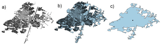
Figure 3.
A typical sequence of image processing used to obtain the structure and shape of street networks, in this case Chillán city (#10, Table 1). (a) The street network directly extracted from public data [50]. (b) A delineation of the network by adopting criteria proposed in [52] and (c) delimitation of the masking area.
By following the observations from Horton [59], when we deal with a perfectly circular shape and for we have squared-shapes. The compactness ratio C measures, instead, the closeness of the object respect to a circular shape. When , we deal with objects of low circularity, and circular or likely circular otherwise. Notice that the definition of C given by Equation (1) is the square root of the circularity index used for fluvial systems. The values of C do not depend on the size of the form [27]. The basin elongation E reads as the ratio of the diameter of a circle of the same area as the basin to the diameter of the system [60], then it is not unusual to classify an urban region from the value of this index, i.e., circular (), oval (), less elongated (), elongated (), and more elongated () [60]. The linear density of the road network is another morphological parameter of interest, that reads as:
where Z is the total length of the streets. This relation is usually adopted for characterising fluvial networks topology [59,61] and it can be interpreted as an Euclidean measure of the degree of saturation of the system.
2.3. Fractal Dimension of Networks
The first formal notion of the topological dimension D of a given set F was given by Hausdorff–Besicovitch [24]. This definition determines this parameter as:
where with , denoting a countable collection of sets covering F ( is the size of each covering subset ). This definition is based on the concept of topological covering of a set, not necessarily connected, leading to fractional dimensions (i.e., non-integer), particularly when dealing with non-Euclidean geometry objects (e.g., Cantor set, Koch curve, Sierpinski set, etc.). Based on this idea, the box-counting method [24] arises as a practical tool frequently applied to measure the fractal dimension of complex systems such as a network. Although some authors have offered some warnings about the reliability of this method [62,63], the box-counting technique can be still considered the best empirical tool to estimate the fractal dimension in almost any complex planar structure [10,11,64].
This method is applied by the software Fractalyse developed at THEMA Laboratory and mostly used for characterizing urban forms [18,22,65]. In the present study, this software was fed with raster and vector images obtained from different SIG data bank [50,51]. Every image was later analyzed by using image-processing tools in QGIS and Matlab software. Figure 3 shows a typical sequence issue from this procedure. Each network can be covered by a finite number of squared-boxes of side s. The box-size s can be reduced step-by-step by following an arithmetic or a geometric progression, increasing the number of boxes covering the figure. According to this method, the fractal dimension of a given network () can be calculated as follows [24,66]:
The parameter can be extracted from the slope of the linear part of the curve vs. . Such linearity is defined into a range of box-sizes, let us say . Beauvais and Montgomery [62] proposed a method to properly chose this range avoiding finite size effects [67] and leading to values strictly comprised into the range 12. In Fractalyse, these points can be easily chosen. Given the variable map scales of our images, the next limits were defined, 1 m. and 2048 m. The choice of agrees with the minimum resolution of each image. With these assumptions, the values of were estimated within a 95% confidence band, with an associated mean error denoted by . This dimension was calculated for map scales ranging from 1:25,000 to 1:500,000. Notice that the variability of is almost negligible into the range 1:50,000 to 1:250,000 as observed in Figure 4, suggesting an appropriate scale to analyse these networks. According to this criterion, the scale 1:100,000 was finally adopted for this study.
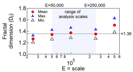
Figure 4.
Variability of for different map scales E. This referential plot corresponds to Chillán (#10 in Table 1). Minimum, average and maximum values of this parameter were included for reference. The horizontal line is a global average.
3. Results
3.1. Morphometry and Patterns of Chilean Street Networks
First, we provide a graphical description about the planar shape of urban forms as depicted in Figure 5. The center of mass of each unit was included for reference (black dots). Arica, Iquique, Antofagasta and La Serena (1, 2, 3 and 5 in Figure 5) are northern cities developing along the coastline. For these entities, the Pacific Ocean becomes a natural frontier limiting their development to the West. These units also locate into desert-like environments where living conditions are adverse for human development (e.g., extreme water scarcity, high temperatures during the day, extreme cold during the night, etc.). The expansion of these cities essentially occurs in the north–south direction, leaving only very small settlements and villages to expand towards inner valleys. On the other hand, as a consequence of poor land-urban planning several precarious settlements are observed in local ravines. These places are, however, exposed to large-scale debris flow risks issue from intense rains during the summer, making these living conditions a typical picture of the north and extreme north of the country. Towards the center of Chile, urbanization increases notoriously. This is the case of Santiago, Rancagua and Valparaíso (see 6, 7 and 8 in Figure 5). Except for this last city, one of the most important ports in the country, most cities in the center tend to develop in valleys around rivers. Santiago and Rancagua show a radial-like expansion with a downtown very strong in commerce and services. This type of expansion was inherited from the historical process of foundation and conquest. Most of the inner migratory fluxes towards this area are explained by its high concentration of schools, universities, companies and industries.
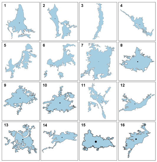
Figure 5.
Shape of Chilean cities analysed in the present study. 1. Arica, 2. Iquique, 3. Antofagasta, 4. Copiapo, 5. La Serena, 6. Valparaiso, 7. Santiago, 8. Rancagua, 9. Talca, 10. Chillan, 11. Concepción, 12. Temuco, 13. Valdivia, 14. Puerto Montt, 15. Coyhaique and 16. Punta Arenas (the center of mass was drawn as black points).
Towards the south of the country cities, large and small, show limited spatial development due to the effects of cordillera de la Costa. This is the case for Concepción, Valdiva and Puerto Montt (11, 13 and 14 in Figure 5). Dendritic forms, as those described by Batty and Longley [9,13], can also be observed in this case. Most of these cities also develop around rivers. Temuco (12 in Figure 5) is another city developing around a river stream, although it growths far from the coast. This city is strongly influenced by indigenous culture developing in a relatively flat landscape, whose expansion is not limited by geographical effects. This city is one of the poorest in the country currently affected by internal guerrillas and terrorism, prompting migratory fluxes to other cities and deceleration of the urbanization process.
In austral regions, the territory is disaggregated forming a very discontinuous landscape. This has significantly limited the possibilities of expansion for many of these cities, as in the cases of Coyhaique and Punta Arenas (15 and 16 in Figure 5). The area and population of these entities are lower than many of the cities of the cadaster and they have not evolved significantly over the last 30 years. These units are still affected by the effects of poor connectivity in the country, which is particularly notorious to the south of the city of Puerto Montt. The urban complexity of these entities is low, the climate is hostile and the level of services is precarious and expensive, making them unattractive for prompting migratory fluxes to these regions. Finally, the cities of Copiapó, Talca and Chillan can be observed in the same figure (4, 9 and 10). These cities grow up into the Central Depression, one the macro-forms of Chilean landscape, and they do not have major geographical restrictions to expand except by Copiapó, which is limited by the presence of mountains and Copiapo River where intense agricultural activity is carried out. Talca and Chillan show radial growth patterns that are also typical of plain areas, as also revealed by Santiago or Rancagua.
Figure 6 shows some street network patterns. Figure 6a, Figure 6k, Figure 6h and Figure 6b show the grids extracted from Arica, Iquique, Antofagasta and La Serena, respectively. These entities show an almost homogeneous distribution of its built area, except by La Serena that shows some signs of density concentration towards the upper sectors, leaving the coast less populated. These features are also shared by Valparaíso (Figure 6e). This city mostly organizes over its surrounding hills and both, population and construction area, decreases towards the coastline, particularly around the port that today suffers a gentrification phenomenon. Camps and middle-class neighborhoods prolifer over the hills, where poverty, precariousness and social insecurity dominate. In addition, a general abandonment state of the city is observed throughout the region, inducing inner migratory displacements towards the nearest city, Viña del Mar. All these elements have significantly contributed to shape the current state of street networks, not only in Valparaiso, but in the whole country as a consequence of the accelerated growth of Chile during the last 30 years. This characteristic was mentioned by Bettencourt [32].
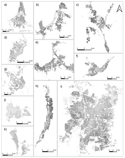
Figure 6.
Network patterns of Chilean cities. (a) Arica, (b) La Serena, (c) Concepción, (d) Punta Arenas, (e) Valparaíso, (f) Temuco, (g) Valdivia, (h) Antofagasta, (i) Santiago, (j) Coyhaique, (k) Iquique. The map scale is E = 1:100,000.
Figure 6c, Figure 6f and Figure 6g show the grid patterns of Concepción, Temuco and Valdivia, respectively. Once again, no significant concentration poles can be observed in Temuco due to the relatively flat character of its urban landscape. However, isolated growth poles do appear in Concepción, Valdivia and Puerto Montt which exhibit a fingering-like pattern. This growing pattern explains by a phenomenon called diffusion-limited aggregation described by Batty [12]. Once again, in these cities educational and commercial activities are concentrated downtown. Remote urban poles are also explained by the presence of important industries related to timber and steel production and manufacturing, although sometimes with high environmental costs. These cities also grow around large rivers that have served to improve people’s life quality, tourism activities and land-valuation, pushing intense building activity around it. It is also important to point out that most of the regions showing growing poles far from downtown, frequently show serious transport connectivity issues. This characteristic has pushed people to use private transport (e.g., cars, motorcycles), contributing to increased country-wide motorization rates and the pollution and saturation of cities. Figure 6d,j show the networks of Coyhaique and Punta Arenas. These entities are of very low complexity as discussed in Section 1.1.
Finally, Figure 6i shows the network pattern of Santiago. The contrasts with the rest of units is clear. This city shows a visibly higher urban density, with radial-like expansion directions. In general, Santiago has grown in a flat valley surrounded by hills, two of them depicted in the same plot (large white gaps in the northeast and southwest. The public transport connectivity works reasonably well particularly near downtown, but its quality and frequency decreases to the periphery. The structure of the city has pushed the appearance of social segregation poles. The wealthiest social classes have moved towards the northeast sectors, while middle classes have settled in central cordons and over the periphery. This peripheral band also concentrates the poorest and vulnerable social groups, particularly in the extreme north and south sectors. These sectors group marginal neighborhoods, where precariousness, social insecurity and a lack of good-quality health and education services become a daily picture. In addition, over the past decades a strong phenomenon of organised crime has emerged there, such that several neighborhoods are today dominated by the presence of gang members closely related with theft and drug dealing activities. In addition, large groups of foreign migrants have settled there, issues from the collapse of migratory regulations. These new phenomena have negatively impacted the interest of the private sector to invest in them and create better projects for housing purposes. The progress of these regions has been then relegated almost exclusively to the role of public institutions.
Table 2 reports the perimeter P, area A, morphological indices and for large and small cities and Figure 7 compares these parameters. Figure 7a, for instance, shows the frequency distribution of . Two significant peaks of index E arise in this plot, one at E = 0.4 and another one at . However, F and C show only one peak at . In addition, Figure 7b reveals that these indices do not show a large variability when compared with A, leading to the mean values 0.52 ± 0.16, 0.23 ± 0.14 and 0.18 ± 0.05, for , respectively. Whatever the case, both plots indicate that the shapes of Chilean cities are very irregular and complex, very influenced by topographical factor, the development of natural frontiers and proximity to the capital of the country. In addition, Table 2 also included the estimation of the box-counting fractal dimension . No significant correlations arise when comparing with network’s density and the morphological indices already introduced, within an arbitrary ±10% scattering band (cf. Figure 7c,d). This behaviour suggests that the fractal dimension is an index evolving almost independently of the remaining morphometric indices.
Table 2.
Morphometric indices of Chilean cities ordered from north to south.
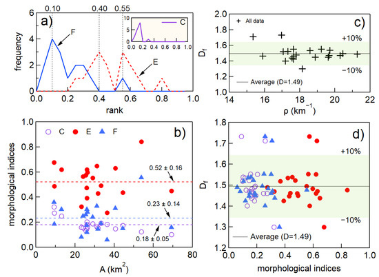
Figure 7.
(a) Frequency distribution of morphological indices . (b) Parameters versus the area of each network A. (c) versus and (d) versus . The horizontal lines are global averages to data. The shadowed region (in green) is an arbitrary ±10% scattering band.
3.2. Fractality of Urban Networks
In this section, we show that some quantitative and graphical relations can be established by analysing the variables introduced in Table 2, by following the guidelines proposed by Shen [26] and Bettencourt [32]. First, Figure 8a compares and the area A of each entity. This area does not considers satellite towns and neighborhoods adjacent to the peripheral of the city. A dataset, obtained from Shen [26] who studied a number of American cities, was included for comparison purposes in the same plot. Once again both sets, Chilean and American cities, can be well characterized by the next fit:
where are fitting parameters estimated with the software IGOR Pro. For Chilean networks we obtain the values , whereas Shen [26] reported . The values obtained for Chilean cities are strictly valid into the range 9.5 km2 ≤ A ≤ 782.5 km2. In addition, the relation between population and area of Chilean cities was depicted in Figure 8a (see inset). In this case, both variables can be fit by a power-law function of the type , where and 1.12. An interesting feature of this comparison is that the slope is different between Chilean and American cities, intercepting at km2, such that for the fractal dimension measured in American cities exceeds the values of Chilean entities. Notice that around the same point , a slight asymmetry on the population distribution arises. The fractal dimension of networks also displays a significant concentration into the range 20 km2 100 km2, leaving two isolated points at the head and tail of the plot. In general, it is possible to conclude that the most populated cities present higher fractality indices as a result of higher levels of complexity and urbanization, leaving the rest of the cities with lower complexity degrees where the fractal dimension is relatively homogeneous. This pattern shows how asymmetric the economic and urban development in the country is, as remarked by Lopez [68].
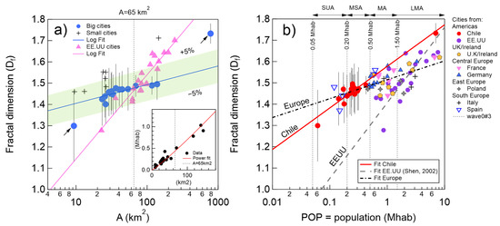
Figure 8.
(a) Relation between vs. for all the entities. Data obtained from [25,26] were included for comparison. Straight lines are given by Equation (6) (SUA = small urban areas, MSA = mid-size urban areas, MA = metropolitan areas, LMA = large-metropolitan areas; according to [69]). (b) Relation between vs. A. American cities were included for comparison. Continuous lines are given by Equation (7) (inset: vs. area A; Mhab = millions of inhabitants. Continuous line is given by , with fitting parameters.)
A similar exercise can be conducted when comparing the fractal dimension and the population of each city, another significant variable of urban development. A clear ordering pattern also arises between both variables as depicted in the plot of Figure 8. Error bands were included for reference, as well as data obtained from some developed cities extracted from the studies from Shen [26] and Lagarias [25]. Once again, both datasets can be fitted by the next function:
where are fitting parameters. Meanwhile for Chilean networks, we obtain the values (1.51,0.11), on the other side we obtain and for American and European cities, respectively. The relations presented in Equations (6) and (7) were also reported by Shen and Bettencourt [26,32]. However, the slope of the curve is once again different for every dataset. According to Batty et al. [14], this parameter can be interpreted as a population saturation rate of the territory, showing different degrees of urban land use. Coincidentally, only Spanish cities fall within the fit calculated for Chilean dataset (given by the continuous red line), maybe explained by historical arguments described in Section 1.1. On the other hand, most of Chilean networks can be classified as small and mid-sized urban areas, that is, SUA and MSA range shown in Figure 8, with only one point in the large-area range (Santiago). The fractal dimension of Chilean units distributes shows large differences from one kind of city to another. This feature is not necessarily observed in developed cities dataset included in this study, which shows a more uniform spread.
From the previous results, it is clear that area and population are two variables closely correlated with the fractal dimension of networks. Both variables give rise to a new parameter called built area to population elasticity [32] defined as:
The concept of elasticity of demand is a parameter of interest in economics and refers to the degree to which demand responds to a change in an economic factor. According to Bettencourt [32] this parameter can be adapted for a better comprehension in the context of city science. Equation (8) leads to the value for Chilean urban forms. However, Molinero and Thurner [70] reported for European cities, whereas the American cities explored in this research lead to . Therefore, by one hand, clear differences on this parameter can be observed from one region to another. However, on the other hand, if American cities show that , for Chilean cities we obtain . The first case suggests that the relation area/population demand follows an elastic-like behavior, whereas the second one, indicates that population changes faster than built area. This last feature can be interpreted as a weakness of market conditions to provide proper coverage to housing demand. In the case of Chile, such features can be easily corroborated throughout territory, worsening in recent decades due to weak public policies incapable of prompting local market conditions and public–private alliances to provide sufficient housing to social groups that cannot access to bank loans. This observation has been objectively corroborated by Castillo and Forray [71].
3.3. Allometric Laws for Chilean Cities
If in the previous section we showed that the fractal dimension is closely related to the urban area and the population of each city, in this section we show that it is possible to establish allometric relationships between some of the geomorphic parameters introduced in Table 2 and the area of each entity. To this concern, Figure 9 displays some scaling laws obtained from the analysis of urban forms in Chile. In particular, Figure 9a,b suggest that the diameter and perimeter of each entity can be fitted by the next generalized function:
where is a characteristic length of the network ( or P), A the area of each city and new fitting parameters. When the next values were obtained (see Figure 9a). Hack’s law [72] was included in the same plot for comparison. Surprisingly, Hack’s coefficients, , are closer to the present measurements. To this concern, it is interesting to recall that Hack’s law was obtained from the analysis of streams networks, by considering as the length of the mainstream. When (Figure 9b), the values were obtained. In this case, the exponent n is even closer to Hack’s exponent.
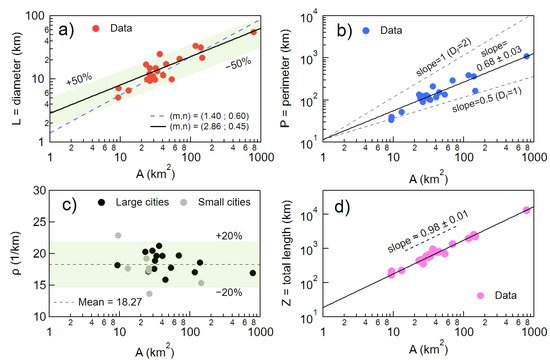
Figure 9.
Allometry of Chilean cities. Relationship between area A and (a) the diameter of each network L, (b) the envelope perimeter P, (c) the the linear density and (d) the total length of each network Z. Shadowed regions (in green) are arbitrary scattering bands. Continuous lines are power-law fitting functions to data.
Figure 9c,d plot the relation between and Z versus A, where Z is the total length of roads of each network. In particular, Figure 9d it follows that:
where . This last value is very close to 1, such that . From Equation (3), it is readily deduced that , where C is a constant. Figure 9c supports this scaling into a ±20% arbitrary scattering band, such that 15.9 km−1 21.3 km−1, suggesting that is an almost homogeneous parameter across the country.
According to Batty [9], the exponent involved on Equation (9) is related to the fractal dimension of the present collection of networks, , in the form . This parameter can be interpreted as a rough measure of the overall fractal degree of such collection. If such a set is constituted by pure fractals objects, that overall value should be the same regardless of the calculation method. To this concern, two additional estimators were introduced for comparison, let us say . All these parameters are defined as follows:
where N is the size of dataset. When 16 we obtain , and ; whereas 1.495 and for (the total data of this study). Then, no significant differences arise when increasing sample’s size (N), but a significant departure can be observed from one estimator to another, such that for . This result reveals that the geometrical features of urban forms considered in this study are far from thos observed in pure fractals (e.g., Cantor, Koch curves set). Indeed, their characteristics are closer to those typically observed in self-affine structures, an observation recently remarked by Martinez et al. [73] working with natural networks in Chile.
Finally, Figure 10 compares and the gross domestic product () differentiated by region (Figure 10a) and by country (Figure 10b). In both cases , characterised by slight positive slope fits. This behaviour reflects that high-income regions usually lead to increasing demands for territorial expansion and then, an increasing degree about the complexity of the systems. This observation has been supported by Batty et al. [9]. Paradoxically, Santiago (R.M.), Antogafasta and Calama do not fall into the fitting curve shown in Figure 10a, even though these two last ones contribute the most to Chile’s GDP, due to intense mining industry activities. However, such contribution has not resulted in significant urban expansion, nor an improvement of the public infrastructure in those regions [74]. This feature is shared by many cities in the country and it is reasonably well captured by the fractal dimension. Figure 10b shows once again a positive correlation between and the global income of countries, where Chile remains at the tail of the distribution.
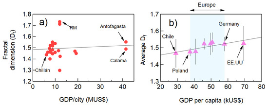
Figure 10.
versus the Gross Domestic Product () at (a) regional level and (b) by country (the parameter was used for these estimations).
4. Discussion
In this study, the box-counting method was applied for estimating the fractal dimension of numerous urban networks distributed throughout the Chilean territory. This method presents as a reliable and robust predictor of this parameter as remarked by D’Acci et al. [10]. We have shown that the fractal dimension is significantly correlated with the area (A) and population () of urban structures as depicted in Figure 8. In total, two fits were proposed to characterize such correlations (Equations (6) and (7)). Although similar fits were already proposed in the literature (see e.g., [26,32]), they are governed by different slopes. This simple result reveals that Chilean cities have progressively occupied the territory at variable saturation rates, which at the same time depend on the local topographical and industrialisation conditions. In addition, the governing parameters of these fits are different compared to similar structures observed in developed countries, suggesting that local cultural and economical factors also help to shape the structure of urban forms. In Chile, the current shape of street networks was the result of an accelerated, but inorganic growing process, particularly during the 20th century. This process still presents serious vulnerabilities owing to poor application of efficient land-use public policies.
In the same context, if urban structures in developed cities expand showing good level of territorial connectivity, good transportation systems and high levels of industrialisation, this is not necessarily the situation observed in developing regions. On the other hand, developed cities try to avoid as much as possible, the appearance of exclusion poles. However, although the Chilean state has strongly fought against poverty and social segregation, social ghettos still remain in peripheral areas of Santiago (the capital) and in many other cities. These asymmetries, inherited since the country’s foundation, have led to strong concentration of services, companies, industries and public institutions in the capital, leaving remote regions under a permanent state of under-development.
To emphasize these characteristics, Figure 11 displays the longitudinal distribution of different metrics, with Santiago (R.M.) playing the role of a center of coordinates and x the distance to Santiago (indicated in Table 1). Figure 11a shows that there is no significant variability of the fractal dimension with respect to x, except for Santiago, Punta Arenas and Coyhaique (the austral cities). The low values of for these last forms are in agreement with their low level of development, by contrast the rest of dimensions show almost similar values. Figure 11b,c show that population and area also increase towards Santiago, a consequence of the concentration of services already mentioned. Such an effect is particularly notorious within the range −1000 km 1000 km. Figure 11d shows that linear density is slightly higher for northern cities, which houses most of the country’s population.
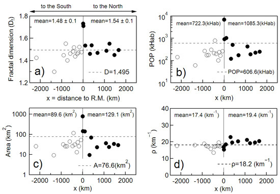
Figure 11.
Longitudinal distribution of different metrics ( for RM.; for northern cities and for southern cities). (a) , (b) (measured in thousands of people ), (c) A and (d) . Global averages were included for reference (dashed lines).
Regarding the morphometry of Chilean urban forms, the indices introduced indicated in Table 2, e.g., , show that Chilean cities display very amorphous shapes. This feature can be easily corroborated in Figure 5 and Figure 6. These last figures also suggest that elongated patterns are the dominant feature of these networks, explained by the strong influence imposed by natural barriers along the territory as the Pacific Ocean to the West, Cordillera de la Costa and Central Depression and Cordillera de los Andes to the East. Then, urban patterns are not only ruled by economical restrictions, but also by the action of the natural characteristics of landscape, together with local environmental characteristics of each region, (e.g., climate, local culture, connectivity, quality of life).
Concerning Equation (10), functional relations of this type have been used for describing the topological structure of fluvial networks [75,76] stating that , where can be seen, once again, as another estimator of the overall fractal dimension of a given collection of structures. If this formula is accepted for this study, it yields to the value . This last one is indeed very close to two suggesting that these systems saturate the available territory in accordance with the space-fillingconcept proposed by Phillips [77]. However, this result contradicts once again the variability of the parameter , whose values are strictly lower than two. Subsequently, although Equation (10) reveals clear ordering patterns for the present urban forms, an overall fractal degree cannot be obtained from this relation.
Following this discussion, the results obtained from Equation (11) emphasize the idea that urban forms behave as self-affine fractal structures, more than self-similar objects. The factors already discussed could explain these patterns. Despite these characteristics, the similarities observed in the structure of urban and natural networks are no less surprising. For example, if the diffusion mechanisms involved in a river network are controlled by natural forces, (e.g., the hydrological cycle, climate influence or the erosive power of streams), the diffusion of an urban form is essentially governed by the need for territorial expansion, land availability, land use, income distribution and rules imposed by public policies, among many other factors. The comprehension about the origin of such similarities, also observed when studying the topology of supply water systems [78], still remains an open question in network science [79].
Finally, it was shown that through the application of routine fractal metrics, it is feasible to obtain significant information about the territorial organization of cities in Chile, in a practical, simple and economical way. This country, still considered as a developing region, can be seen as an interesting source of information in South America for comparing existing databases, most of them built from data obtained in developed contexts. Although some quantitative relations hold, fractal metrics help to describe some asymmetries about urban development arising throughout Chilean territory and an inelastic-like behaviour with respect to area/population demand, that is, in Chile, the population grows faster than the rate areas are built, and public policies have failed to avoid the effects of this phenomenon. Indeed, the current situation of the country still shows a strong degree of concentration in the capital and some nearby cities. However, a poor urban development and connectivity remains further away, particularly at extreme northern and southern regions. These properties are a consequence of the accelerated development of the country in recent decades, but also of some deficits in the construction of an efficient, intelligent and balanced urban planning.
5. Conclusions
Characterizing an urban network is a complex task that can be reasonably achieved with fractal metrics. In this case study, we show that fractal theory provides valuable information about the spatial organization of cities in a simple, quick, and cost-effective manner. This is the first significant effort to provide a fractal characterization of Chilean urban networks by measuring the box-counting fractal dimension of different Chilean cities, together with morphometric indices typically used for characterizing branched structures. These cities display different degrees of fractality, a sign of unequal expansion rates and land-use planning across the country. Such characteristics can be explained by an asymmetric distribution of services, location of industrialisation degree, employment possibilities and quality of life from one region to another. These differences have also induced rural–urban migration disputing territories and resources associated with industrial processes and extractive functions such as mining and agriculture, while leaving extreme cities in a persistent state of isolation and poor development. In addition, strong correlations were observed between fractal dimension, area and population. Although some of them were already reported in the literature, the parameters involved in them show significant differences between developed and developing countries. Citizen income, private/public investment, market conditions and the cultural and organisational historical heritage have, perhaps, contributed to the current structure of urban forms. A significant correlation with the gross domestic product was also reported, suggesting that the country’s income and the degree of investment in building are important variables behind the development of cities.
With these elements, it is possible to affirm that the current shape of Chilean urban networks is the combined result of many factors (culture, economics, public policies) together with the action of natural barriers, imposing clear restrictions for urban expansion. Fractal theory is able to capture these characteristics, leading to reasonable results that help us better understand the spatial organisation of cities in developing countries. However, it is necessary to mention some limitations of these metrics. First, all of the analyses conducted consider planar structures; however, cities expand in all spatial directions. Consequently, when we discuss fractality we must also consider how cities expand in the vertical direction as reported by Dupuy [13]. Another limitation of this study relates to the time-evolution of cities. The fractal degree of a city must also take into account how urban structures, territorial expansion, land use, and population mobility evolve over time. A dedicated study focusing on the variability of these parameters could significantly help to better understand how market conditions, economics, population mobility and environmental conditions have shaped the current state of cities. Finally, in this study we assign a single value of fractality to each city, assuming that these structures behave as homogeneous structures. Nevertheless, this is a simplistic approach. Cities also develop showing different geometrical structures into a given network. Perhaps a multi-fractal analysis and the determination of additional indices as the ht-index proposed by Jiang [80,81] could help in this regard, and will certainly represent the focus of a future study.
Author Contributions
Conceptualization, F.M.; methodology, F.M. and H.M.; software, F.M.; validation, B.S. and F.M.; formal analysis, F.M. and H.M.; investigation, F.M. and B.S.; resources, F.M.; data curation, F.M. and H.M.; writing—original draft preparation, F.M. and H.M.; writing—review and editing, F.M. and H.M.; supervision, F.M.; project administration, F.M.; funding acquisition, F.M. All authors have read and agreed to the published version of the manuscript.
Funding
This study was funded by the grant Investigador Emergente, Code 039.329/2022, from Vicerrectoría de Investigación of the Pontificia Universidad Católica de Valparaíso, Chile.
Informed Consent Statement
Not applicable.
Data Availability Statement
The data are available from the first author upon reasonable request.
Acknowledgments
The authors acknowledge the School of Civil Engineering from PUCV for supporting this research.
Conflicts of Interest
The authors declare no conflict of interest.
References
- Feder, J. Fractals; Physics of Solids and Liquids, Plenum Press: New York, NY, USA, 1988. [Google Scholar]
- Bunde, A.; Havlin, S. Fractals and Disordered Systems; Springer Science & Business Media: Norwell, MA, USA, 2012. [Google Scholar]
- Bunde, A.; Havlin, S. Fractals in Science; Springer: Berlin/Heidelberg, Germany, 2013. [Google Scholar]
- Mandelbrot, B. The Fractal Geometry of Nature; WH Freeman: New York, NY, USA, 1982. [Google Scholar]
- Gouyet, J.F. Physics and Fractal Structures; Elsevier Masson: Paris, France, 1996. [Google Scholar]
- Turcotte, D.L. Fractals in geology and geophysics. Pure Appl. Geophys. 1989, 131, 171–196. [Google Scholar] [CrossRef]
- Mandelbrot, B. How long is the coast of Britain? Statistical self-similarity and fractional dimension. Science 1967, 156, 636–638. [Google Scholar] [CrossRef] [PubMed]
- Scholz, C.H.; Mandelbrot, B.B. Fractals in Geophysics; Springer: Berlin/Heidelberg, Germany, 1989. [Google Scholar]
- Batty, M.; Longley, P.A. Fractal Cities: A Geometry of Form and Function; Academic Press: Cambridge, MA, USA, 1994. [Google Scholar]
- D’Acci, L.; Batty, M. The Mathematics of Urban Morphology; Springer: Berlin/Heidelberg, Germany, 2019. [Google Scholar]
- Chen, Y. Fractal Modeling and fractal dimension description of urban morphology. Entropy 2020, 22, 961. [Google Scholar] [CrossRef] [PubMed]
- Batty, M.; Longley, P.; Fotheringham, S. Urban growth and form: Scaling, fractal geometry, and diffusion-limited aggregation. Environ. Plan. A 1989, 21, 1447–1472. [Google Scholar] [CrossRef]
- Dupuy, G. Villes, Réseaux et Transport: Le Défi Fractal; Economica: Bonn, Germany, 2017. [Google Scholar]
- Batty, M.; Xie, Y. Preliminary evidence for a theory of the fractal city. Environ. Plan. A 1996, 28, 1745–1762. [Google Scholar] [CrossRef]
- Batty, M. Cities and Complexity: Understanding Cities with Cellular Automata, Agent-Based Models, and Fractals; The MIT Press: Cambridge, MA, USA, 2007. [Google Scholar]
- Frankhauser, P. Aspects fractals des structures urbaines. L’Espace GéOgraphique 1990, 45–69. [Google Scholar] [CrossRef]
- Frankhauser, P. La Fractalité des Structures Urbaines. Ph.D. Thesis, Anthropos, Paris, France, 1993. [Google Scholar]
- Frankhauser, P. Fractal geometry for measuring and modelling urban patterns. In The Dynamics of Complex Urban Systems; Springer: Berlin/Heidelberg, Germany, 2008; pp. 213–243. [Google Scholar]
- White, R.; Engelen, G. Urban systems dynamics and cellular automata: Fractal structures between order and chaos. Chaos Solitons Fractals 1994, 4, 563–583. [Google Scholar] [CrossRef]
- Thomas, I.; Frankhauser, P.; De Keersmaecker, M.L. Fractal dimension versus density of built-up surfaces in the periphery of Brussels. Pap. Reg. Sci. 2007, 86, 287–308. [Google Scholar] [CrossRef]
- Thomas, I.; Frankhauser, P.; Biernacki, C. The morphology of built-up landscapes in Wallonia (Belgium): A classification using fractal indices. Landsc. Urban Plan. 2008, 84, 99–115. [Google Scholar] [CrossRef]
- Thomas, I.; Frankhauser, P.; Badariotti, D. Comparing the fractality of European urban neighbourhoods: Do national contexts matter? J. Geogr. Syst. 2012, 14, 189–208. [Google Scholar] [CrossRef]
- Tannier, C. About Fractal Models in Urban Geography and Planning: Refuting the Aesthetics and The Universal Norm, 2018. Blog Post on ‘Cybergeo Conversation’. 13 March 2018. Available online: https://cybergeo.hypotheses.org/223 (accessed on 11 October 2022).
- Falconer, K. Fractal geometry: Mathematical Foundations and Applications; John Wiley & Sons: Hoboken, NJ, USA, 2004. [Google Scholar]
- Lagarias, A.; Prastacos, P. Fractal dimension of European Cities: A comparison of the patterns of built-up areas in the urban core and the peri-urban ring. Cybergeo Eur. J. Geogr. 2021, 987, 37243. [Google Scholar] [CrossRef]
- Shen, G. Fractal dimension and fractal growth of urbanized areas. Int. J. Geogr. Inf. Sci. 2002, 16, 419–437. [Google Scholar] [CrossRef]
- Rodin, V.; Rodina, E. The fractal dimension of Tokyo’s streets. Fractals 2000, 8, 413–418. [Google Scholar] [CrossRef]
- Feng, J.; Chen, Y. Spatiotemporal evolution of urban form and land-use structure in Hangzhou, China: Evidence from fractals. Environ. Plan. Plan. Des. 2010, 37, 838–856. [Google Scholar] [CrossRef]
- Jahanmiri, F.; Parker, D.C. An Overview of Fractal Geometry Applied to Urban Planning. Land 2022, 11, 475. [Google Scholar] [CrossRef]
- Marshall, S. Streets and Patterns; Routledge: London, UK, 2004. [Google Scholar]
- Oliveira, V. Urban Morphology: An Introduction to the Study of the Physical Form of Cities; Springer: Berlin/Heidelberg, Germany, 2016. [Google Scholar]
- Bettencourt, L.M. Introduction to Urban Science: Evidence and Theory of Cities as Complex Systems; MIT Press: Cambridge, MA, USA, 2021. [Google Scholar]
- International Monetary Fund. World Economic Outlook Database. 2022. Available online: https://www.imf.org/en/Publications/WEO/weo-database/2022/April/select-country-group (accessed on 11 October 2022).
- Nuñez, J.; Tartakowsky, A. Inequality of Outcomes vs. Inequality of Opportunities in a Developing Country. An exploratory analysis for Chile. Estud. Econ. 2007, 34, 185–202. [Google Scholar]
- Zhao, C.; Li, Y.; Weng, M. A Fractal Approach to Urban Boundary Delineation Based on Raster Land Use Maps: A Case of Shanghai, China. Land 2021, 10, 941. [Google Scholar] [CrossRef]
- Purevtseren, M.; Tsegmid, B.; Indra, M.; Sugar, M. The fractal geometry of urban land use: The case of Ulaanbaatar city, Mongolia. Land 2018, 7, 67. [Google Scholar] [CrossRef]
- Ma, D.; Guo, R.; Zheng, Y.; Zhao, Z.; He, F.; Zhu, W. Understanding Chinese urban form: The universal fractal pattern of street networks over 298 cities. ISPRS Int. J. Geo-Inf. 2020, 9, 192. [Google Scholar] [CrossRef]
- Karpinski, M.; Kuznichenko, S.; Kazakova, N.; Fraze-Frazenko, O.; Jancarczyk, D. Geospatial Assessment of the Territorial Road Network by Fractal Method. Future Internet 2020, 12, 201. [Google Scholar] [CrossRef]
- Bodini, H. Geografía Urbana de Chile; Instituto Geográfico Militar, Colección Geografía de Chile: Santiago, Chile, 1985; Volume 10. [Google Scholar]
- De Ramón, A. Suburbios y arrabales en un área metropolitana. El caso de Santiago de Chile, 1872–1932. In Ensayos Histórico-Sociales Sobre la Urbanización en América Latina; Hardoy, J.E., Morse, R.M., Schaedel, R.P., Eds.; Ediciones SIAP· CLACSO: Buenos Aires, Argentina, 1978. [Google Scholar]
- Cadaster of Camps in Chile, El Mercurio. Available online: https://www.emol.com/noticias/Economia/2018/12/26/932200/Gobierno-elabora-nuevo-catastro-de-campamentos-en-Chile.html (accessed on 24 October 2022).
- Fundación Ingeniería Sin Fronteras Chile, Proyecto “Escuela Dignidad, Etapa 4 Campamento Dignidad” (2021), La Florida, Región Metropolitana. Available online: https://isf-chile.org/portfolio/proyecto-escuela-dignidad-etapa-1/ (accessed on 24 October 2022).
- Vergara, L. Convivencia y conflictos en barrios de ingresos mixtos. BitáCora Urbano Territ. 2021, 31, 41–52. [Google Scholar] [CrossRef]
- Vista de Las Condes desde la Gran Torre Santiago. Available online: https://es.wikipedia.org/wiki/Sector_nororiente_de_Santiago (accessed on 24 October 2022).
- Manríquez, M.T.; Cáceres, D.F.; Jiménez, D.G. Reforma Agraria en Chile, ¿Palimpsesto de otra ruralidad? Reflexiones y propuestas. Polis. Rev. Latinoam. 2017, 47, 432. [Google Scholar] [CrossRef]
- La Reforma Agraria (1962–1973). Available online: https://www.memoriachilena.gob.cl/602/w3-article-3536.html#presentacion (accessed on 24 October 2022).
- Martínez Pizarro, J. Urbanización, Crecimiento Urbano y Dinámica de la población de las principales ciudades de Chile entre 1952 y 1992. Rev. Geogr. Norte Gd. 1997, 24, 23–30. [Google Scholar]
- Martínez Pizarro, J. Ciudades de Chile, migración interna y redistribución de la población: Algunas evidencias del período 1987–1992. Rev. Geogr. Norte Gd. 2002, 29, 21–38. [Google Scholar]
- Fuentes Arce, L. Competitividad urbana en el contexto latinoamericano: El caso de Santiago de Chile. Rev. Geogr. Norte Gd. 2011, 48, 81–106. [Google Scholar] [CrossRef]
- Ministerio de Bienes Nacionales de Chile, Infraestructura de Datos Geoespaciales (IDE). Red Vial Nacional. 2019. Available online: https://www.ide.cl/index.php/transporte/item/1708-red-vial-nacional (accessed on 5 October 2022).
- Ministerio de Bienes Nacionales de Chile, Infraestructura de Datos Geoespaciales (IDE). ¿Qué es el IDE Chile? 2022. Available online: https://www.ide.cl/ (accessed on 5 October 2022). (In Spanish).
- Ministerio de Bienes Nacionales de Chile, Infraestructura de Datos Geoespaciales (IDE). Área Urbana Consolidada. 2016. Available online: https://www.ide.cl/index.php/planificacion-y-catastro/item/1845-area-urbana-consolidada (accessed on 5 October 2022). (In Spanish).
- Observatorio Social—Ministerio de Desarrollo Social y Familia. Estimación de Tasa de Pobreza por Ingreso por Comuna. 2020. Available online: http://observatorio.ministeriodesarrollosocial.gob.cl/pobreza-comunal-2020 (accessed on 5 October 2022). (In Spanish).
- Observatorio del Sistema Nacional de Ciencia, Tecnología y Conocimiento e Innovación, Ministerio de Ciencias de Chile. PIB Total y per Cápita Regional. 2020. Available online: https://observa.minciencia.gob.cl/indicadores/contexto-socioeconomico/pib-per-capita-regional (accessed on 5 October 2022). (In Spanish).
- Ferreira, J.A.; Condessa, B.; e Almeida, J.C.; Pinto, P. Urban settlements delimitation in low-density areas—An application to the municipality of Tomar (Portugal). Landsc. Urban Plan. 2010, 97, 156–167. [Google Scholar] [CrossRef]
- Gregory, K.; Gregory, P.; Walling, D. Drainage Basin Form and Process: A Geomorphological Approach; Wiley: Hoboken, NJ, USA, 1973. [Google Scholar]
- Zavoianu, I. Morphometry of Drainage Basins; Elsevier: Amsterdam, The Netherlands, 2011. [Google Scholar]
- Rudin, W. Principles of Mathematical Analysis W. Rudin; McGraw-Hill: New York, NY, USA, 1953. [Google Scholar]
- Horton, R.E. Erosional development of streams and their drainage basins; hydrophysical approach to quantitative morphology. Geol. Soc. Am. Bull. 1945, 56, 275–370. [Google Scholar] [CrossRef]
- Schumm, S.A. Evolution of drainage systems and slopes in badlands at Perth Amboy, New Jersey. Geol. Soc. Am. Bull. 1956, 67, 597–646. [Google Scholar] [CrossRef]
- Strahler, A.N. Part II. Quantitative geomorphology of drainage basins and channel networks. In Handbook of Applied Hydrology; McGraw-Hill: New York, NY, USA, 1964; pp. 4–39. [Google Scholar]
- Beauvais, A.A.; Montgomery, D.R. Are channel networks statistically self-similar? Geology 1997, 25, 1063–1066. [Google Scholar] [CrossRef]
- Cheeseman, A.K.; Vrscay, E.R. Estimating the Fractal Dimensions of Vascular Networks and Other Branching Structures: Some Words of Caution. Mathematics 2022, 10, 839. [Google Scholar] [CrossRef]
- Kusák, M. Methods of fractal geometry used in the study of complex geomorphic networks. AUC Geogr. 2014, 49, 99–110. [Google Scholar] [CrossRef]
- Frankhauser, P. Comparing the morphology of urban patterns in Europe—A fractal approach. Eur.-Cities Insights Outskirts Rep. Cost Action 2004, 10, 79–105. [Google Scholar]
- Rodriguez-Iturbe, I.; Rinaldo, A. Fractal River Basins: Chance and Self-organization; Cambridge University Press: Cambridge, UK, 2001. [Google Scholar]
- Labini, F.S.; Gabrielli, A.; Montuori, M.; Pietronero, L. Finite size effects on the galaxy number counts: Evidence for fractal behavior up to the deepest scale. Phys. A Stat. Mech. Its Appl. 1996, 226, 195–242. [Google Scholar] [CrossRef]
- López, R.; Miller, S.J. Chile: The unbearable burden of inequality. World Dev. 2008, 36, 2679–2695. [Google Scholar] [CrossRef]
- Urban Population by City Size, OCDE 2020. Available online: https://data.oecd.org/popregion/urban-population-by-city-size.htm (accessed on 24 October 2022).
- Molinero, C.; Thurner, S. How the geometry of cities explains urban scaling laws and determines their exponents. arXiv 2019, arXiv:1908.07470. [Google Scholar]
- Castillo, M.J.; Forray, R. La vivienda, un problema de acceso al suelo. Arq (Santiago) 2014, 86, 48–57. [Google Scholar] [CrossRef]
- Hack, J.T. Studies of Longitudinal Stream Profiles in Virginia and Maryland; US Government Printing Office: Washington, DC, USA, 1957; Volume 294.
- Martinez, F.; Manriquez, H.; Ojeda, A.; Olea, G. Organization Patterns of Complex River Networks in Chile: A Fractal Morphology. Mathematics 2022, 10, 1806. [Google Scholar] [CrossRef]
- Leiva Gómez, S.; Parra Calderón, M. La voz de los pobres del Norte Grande de Chile: Estudio sobre la pobreza con participación de los afectados. Rev. Geogr. Norte Gd. 2011, 50, 87–104. [Google Scholar] [CrossRef]
- Dodds, P.S.; Rothman, D.H. Unified view of scaling laws for river networks. Phys. Rev. E 1999, 59, 4865. [Google Scholar] [CrossRef]
- Rosso, R.; Bacchi, B.; La Barbera, P. Fractal relation of mainstream length to catchment area in river networks. Water Resour. Res. 1991, 27, 381–387. [Google Scholar] [CrossRef]
- Phillips, J. Interpreting the fractal dimension of river networks. Fractals Geogr. 1993, 7, 142–157. [Google Scholar]
- Di Nardo, A.; Di Natale, M.; Giudicianni, C.; Greco, R.; Santonastaso, G.F. Complex network and fractal theory for the assessment of water distribution network resilience to pipe failures. Water Sci. Technol. Water Supply 2018, 18, 767–777. [Google Scholar] [CrossRef]
- Network Science. Available online: http://networksciencebook.com/ (accessed on 13 January 2023).
- Jiang, B. Head/tail breaks: A new classification scheme for data with a heavy-tailed distribution. Prof. Geogr. 2013, 65, 482–494. [Google Scholar] [CrossRef]
- Jiang, B.; Yin, J. Ht-index for quantifying the fractal or scaling structure of geographic features. Ann. Assoc. Am. Geogr. 2014, 104, 530–540. [Google Scholar] [CrossRef]


Disclaimer/Publisher’s Note: The statements, opinions and data contained in all publications are solely those of the individual author(s) and contributor(s) and not of MDPI and/or the editor(s). MDPI and/or the editor(s) disclaim responsibility for any injury to people or property resulting from any ideas, methods, instructions or products referred to in the content. |
© 2023 by the authors. Licensee MDPI, Basel, Switzerland. This article is an open access article distributed under the terms and conditions of the Creative Commons Attribution (CC BY) license (https://creativecommons.org/licenses/by/4.0/).