Abstract
Developing appropriate tools to understand and protect ecosystems and the services they provide is of unprecedented importance. This work describes the activity performed by ISPRA for the mapping of the types of ecosystems and the evaluation of their related ecosystem services, to meet the needs of the “ecosystem extent account” and “ecosystem services physical account” activities envisaged by the SEEA-EA framework. A map of the types of ecosystems is proposed, obtained by integrating the main Copernicus data with the ISPRA National Land Consumption Map, according to the MAES (Mapping and Assessment of Ecosystems and their Services) classification system. The crop production and carbon stock values for 2018 were then calculated and aggregated with respect to each ecosystem. The ecosystem accounting was based on the land cover map produced by ISPRA integrating, according to an EAGLE compliant classification system, the same Copernicus and National input data used for mapping the types of ecosystems. The analysis shows the importance of an integrated reading of the main monitoring tools and the advantages in terms of compatibility and comparability, with a view to enhancing the potential of Copernicus land monitoring instruments also in the context of ecosystem accounting activities.
Keywords:
ecosystem accounting; Copernicus; land cover; SEEA-EA; MAES; EAGLE; ecosystem services; carbon stock; crop production 1. Introduction
Ecosystems represent the base units to detect land changes and to assess environmental conditions, which enables the recognition of past and current ecological processes and the related services supplied and the analysis of future scenarios [1,2,3]. The ecosystem’s biotic and abiotic characteristics and state affect the energy flow, the nutrient cycle, and the availability of resources, species, and habitat [4,5,6]. In this sense, an exhaustive, effective, and operational ecosystems distribution knowledge is a fundamental aspect in land monitoring activities [7].
The whole legislative framework settled for by the EU in recent years refers to ecosystem accounting, e.g., the Biodiversity Strategy for 2030 [8] and the related European Soil Strategy [9], the Nature Restoration Law [10] adopted by the Commission in June 2022, and the Healthy Soils Law that is under preparation. The United Nations Statistical Commission, in its 52nd session of March 2021, attributed to the National Accounting System and to the System of Environmental Economic Accounting (SEEA) the assessment of the contribution of the environment to the economy and the impact of the economy on the environment. This is in order to provide data, indicators, and statistics to stakeholders, to monitor these interactions, and to identify more sustainable development strategies. SEEA Ecosystem Accounting (SEEA-EA) is now the reference framework under the proposal for the amendment of Regulation (EU) No. 691/2011 on European environmental economic accounts to include a new module on ecosystem accounts [11]. The proposed legal module on ecosystem accounts has been adopted by the Commission in July 2022 and proposed to the Council and Parliament for final approval. Relevant policies consider the SEEA-EA framework, including the Nature Directives, the Marine Strategy Framework Directive, the Common Agriculture Policy, the EU Forest Strategy, and the EU Pollinators Initiative [12,13,14,15]. The SEEA-EA may also support the reporting under the 8th Environmental Action Programme or the revised Regulation on Land Use Land-Use Change, and Forestry (LULUCF) (EU) 2018/841 [11]; it can also be an example for further analysis models to implement in international projects such as the Horizon 2020 project SERENA (Soil Ecosystem seRvices and soil threats modElling aNd mApping), which is conducting an in-depth analysis of models about soil threats, soil ecosystem services, and their bundles at the European level [16]. The Natural Capital Accounting and Ecosystem Service Valuation (NCAVES) project highlighted the potential of the SEEA-EA in supporting the calculation and mainstreaming of many Aichi target indicators and Sustainable Development Goal (SDG) indicators [17] and the link with other key international environmental conventions and platforms, including the UNCCD, Ramsar, and IPBES [18]. The UN Committee of Experts on Environmental-Economic Accounting (UNCEEA) conducted a “Broad Brush Analysis of SDG Indicators” identifying 40 SEEA-relevant SDG indicators that are or can be aligned with the SEEA [19]. In detail, the usefulness of the SEEA as a tool to mainstream the environment and biodiversity into national planning processes is explicitly recognised via SDG Indicator 15.9.1, “Progress towards national targets established in accordance with Aichi Biodiversity Target 2 of the Strategic Plan for Biodiversity 2011–2020”, which in part B requires the “integration of biodiversity values into national accounting and reporting systems, defined as implementation of the SEEA” [20]. The need to produce systematic physical and monetary measurements of the flow of ecosystem services on a national scale is also expressed at the national level by law 221/2015, which requires the development of consolidated statistical and accounting systems for natural capital and the introduction of indicators for assessing the impact of policies on it.
The SEEA-EA is a spatially based integrated framework conceived to create a coherent and comprehensive view of ecosystems, allowing the organisation of biophysical data, the measurement of ecosystem services, the tracking of changes in ecosystem assets, and the linking of this information to economic aspects and other human activity. The SEEA-EA aims to become the tool for ecosystem accounting globally by standardising data production, thus making it accessible and comparable [21,22,23]. In detail, the following set of accounts is defined [22]:
- Ecosystem extent account, which organises information on the extent of different ecosystem types (e.g., forests, wetlands, agricultural areas, marine areas) as a starting point for ecosystem accounting.
- Ecosystem condition account, which considers the ecological integrity of ecosystems, evaluating the distance from a reference condition with respect to different biophysical characteristics.
- Ecosystem services physical and monetary flow account, which measures the supply and use of ecosystem services by economic units.
- Monetary ecosystem asset account, which evaluates stocks and changes in stocks of ecosystem assets, based on the monetary valuation of ecosystem services at the beginning and end of each accounting period.
- Thematic accounts, which organise data on themes of specific policy relevance, such as biodiversity, climate change, urban areas, and oceans.
In order to provide a comprehensive measurement of Natural Capital and Ecosystem Services, the European Commission initiative MAES (Mapping and Assessment of Ecosystems and their Services) is a strong tool to support the effort to map and classify the extent of ecosystems, providing the conceptual framework, methodologies, and indicators to collect information on ecosystems and their services in Europe, in order to address policy decisions. MAES responded to Action 5 of the European Biodiversity Strategy to 2020, which lays the foundation for the development of a methodology for understanding the condition of biodiversity and ecosystems and the pressures they are subject to. In response to this task, since 2012, the MAES working group has developed a classification system for ecosystems [24], and then deepened the issues related to monitoring and analysis of ecosystem services [2]. The ecosystem classification method proposed in MAES is based on the use of CLC classes aggregated on the basis of the relationships between land cover (LC) and land use (LU) classes and EUNIS habitats in order to represent and collect information on large-scale ecosystems [24]. The result is a 12-class classification system, which gathers 7 terrestrial ecosystems, a freshwater one, and 4 related to marine areas. The ecosystem types proposed in MAES were used for the EU ecosystem extent accounts within the INCA project (The official name of the INCA project is knowledge innovation project on an Integrated system of Natural Capital and ecosystem services Accounting for the European Union), which was used to test the System of Environmental-Economic Accounting-Experimental Ecosystem Accounting (SEEA-EEA). The results were included in the most recent version of the SEEA-EA handbook, adopted in 2021 [25]. In this context, the INCA project has shown that by following the SEEA-EA guidelines, it is possible to produce large amounts of data on ecosystem accounting, thus enabling consistent and comparable information on ecosystems and ecosystem services at the European scale.
The MAES classification system has also been adopted by the Copernicus Land Monitoring Service (CLMS) Local Component (details are available at https://land.copernicus.eu/local, accessed on 11 January 2023), which includes high spatial and thematic resolution vector data relating to three main categories of areas that require specific and detailed monitoring: the Riparian Zones data offer a mapping of riparian areas [26], the Coastal Zones data map a buffer zone of 10 km from the coast line [27], and the Natura 2000 data map protected areas [28]. The Copernicus CLMS also includes other relevant LC/LU products, such as the CORINE Land Cover [29], Urban Atlas [30], and the new CLC Plus Backbone data [31], and also numerous other geographic information on soils and related variables (e.g., the state of the vegetation or the water cycle). One of the objectives of Copernicus is to provide data organised according to criteria that guarantee comparability and interchange between different EU countries. This need is particularly important in the context of LC/LU monitoring, where products born in different contexts and for different needs have required the definition of specific classification systems, which are often difficult to compare. In order to coordinate data flows from a thematic point of view, within CLMS, the EAGLE concept (EIONET Action Group on Land monitoring in Europe) was introduced. EAGLE aims to define a conceptual methodology to describe land cover and land use information from different classification systems by tracing them to the three categories: Land cover components (LCC), Land use attributes (LUA), and Landscape characteristics (CH) [32]. This allows the understanding of overlaps and the possible conversions between different classification systems, but also to define new ones. The EAGLE model aims to separate the LC and LU components through data modelling systems applicable at different scales and in different contexts, while maintaining compatibility with existing datasets.
Over the years, the Italian Institute for Environmental Protection and Research (ISPRA) has introduced many different LC and LU products on a national scale for the Italian territory, as much as possible in line with the EAGLE model, both through the classification of Sentinel-1 and -2 data [33,34,35], and through the integration of existing data. In this sense, a methodology was developed for the integration of Copernicus and national data, which made it possible to produce a national scale EAGLE compliant land cover map starting from the integration of CLMS Local (Coastal Zones, Riparian Zones, Urban Atlas, Natura 2000) and Pan European (CORINE Land Cover, CLC Plus Backbone) LC/LU data with the ISPRA National Land Consumption Map (LCM) [36]. This product overcomes some of the main limitations of the CLC and MAES classification systems, such as the widespread use of mixed LC/LU classes, and makes it possible to meet the needs of SEEA-EA Ecosystem services’ physical accounting, becoming the basis for the assessment of ecosystem service proposed by the annual ISPRA report on land consumption [37].
This research is a first attempt to map the MAES ecosystem types at a national scale, in order to provide support data to the ecosystem extent accounting activity with respect to the classes recognised internationally by SEEA-EA and considered at a national level for the future accounting of ecosystem services. In this sense, a map of the types of ecosystems was produced by integrating the main CLMS data and the LCM, while the ecosystem services associated with crop production and carbon stocks in the soil were calculated and expressed as a function of these types of ecosystems.
2. Materials and Methods
2.1. Overview
The following methodology describes the input data and the procedures adopted to produce a map of the MAES types of ecosystems, useful for the activities of ecosystem extent accounting in compliance with the SEEA-EA approach. The ecosystems thus identified were associated with the values of ecosystem services relating to crop production and carbon storage. The two ecosystem services are estimated with reference to the total stock, starting from the LC map produced that integrated the main CLMS data with the LCM [37] according to an EAGLE compliant classification system. The analysis was conducted for the entire national territory, with reference to 2018 (Figure 1).
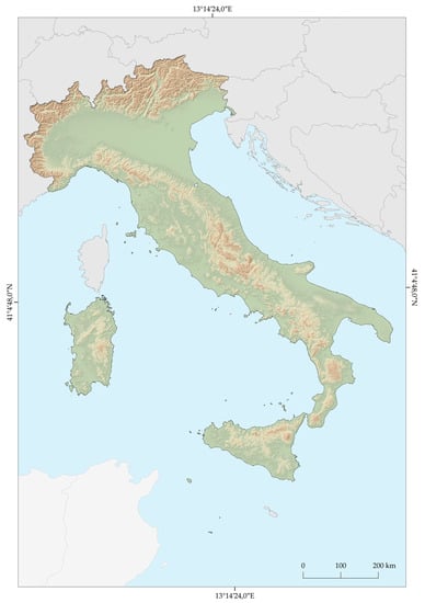
Figure 1.
Study area. The analysis was conducted for the entire Italian national territory.
2.2. SEEA-EA Compliant Types of Ecosystems Map
To produce a map of the ecosystem typologies in compliance with the United Nations SEEA-EA approach [22], the classification system of Table 1 was defined.

Table 1.
MAES ecosystem types adopted for the realisation of the ecosystem type map by integrating Copernicus data with the LCM.
The proposed classification system of the types of ecosystems refers to the MAES classes, which are divided at the first classification level into terrestrial ecosystems, freshwater ecosystems, and marine ecosystems, and then further characterised at the second classification level.
Terrestrial ecosystems are delineated starting from CORINE Land Cover classes and are subdivided into:
- Settlements and other artificial areas, i.e., urban areas where most of the human population live and which also include significant areas for synanthropic species associated with urban habitats. This class significantly affects other ecosystem types and includes urban, industrial, commercial, and transport areas, green urban areas, and mines, dumping, and construction sites.
- Cropland, i.e., areas mainly dedicated to agricultural production, even with the presence of important natural areas.
- Grassland, i.e., areas with a prevalence of herbaceous vegetation, which can include managed pastures and natural and semi-natural pastures.
- Forest and woodland include areas dominated by woody vegetation; they are very important from the point of view of the provision of ecosystem services.
- Heathland and shrub are dominated by moors, heathland, and sclerophyllous vegetation.
- Sparsely vegetated ecosystems are all naturally unvegetated or sparsely vegetated habitats, usually with extreme climatic conditions, such as bare rocks, glaciers, dunes, beaches, and sand plains.
- Inland wetlands include natural or modified mires, bogs, and fens, as well as peat extraction sites. In these areas, water regulation and peat-related processes are associated with specific species of animals and plants.
Freshwater ecosystems include permanent freshwater, inland water courses, and water bodies.
For marine ecosystems, the only class considered was “Marine inlets and transitional water”, which includes coastal wetlands, lagoons, estuaries, i.e., areas on the land–water interface under the influence of tides and with salinity levels greater than 0.5 ‰. The other types of marine ecosystems were not considered as they relate to areas outside the study area; furthermore, they are not considered in CLMS data.
In detail, the map integrates the main local and Pan-European CLMS data and the ISPRA LCM for the year 2018 (Table 2).
Table 2.
Input data used for the mapping of ecosystem types and to produce the land cover map used for the ecosystem services assessment; LC= Land Cover classes, LU= Land Use classes, CLMS= Copernicus Land Monitoring Service.
The input data were reclassified according to ecosystems of Table 1 and merged into a single 10 × 10 m raster mosaic. The proposed typologies represent the basic units for ecosystems state and services assessments from the local to national scale. This map aims to provide a representation of the Italian territory with respect to the MAES classes in order to be a useful support for the ecosystem extent accounting activity.
These ecosystem types have been associated with the values of the services relating to agricultural productivity and organic carbon storage, calculated using the procedure described in the following paragraphs.
2.3. EAGLE Compliant Land Cover for the Assessment of Ecosystem Services
The same input data described before (Table 2) were combined to produce a land cover map for 2018 according to the methodology described in De Fioravante et al. [33].
The input data were converted to a 10 × 10 m resolution raster and reclassified according to the classification system of Table 3, which is based on previous activities of the ISPRA working group [33,36] and adopts a combination of land cover classes directly attributable to the EAGLE model Land Cover Components (LCC), integrated with appropriate Land Characteristics (LCH) in order to increase the thematic detail of the classification system and preserve the information content of the input data.
Table 3.
Land cover map classification system.
At the first classification level, four macro-classes are defined (Abiotic non-vegetated areas, Biotic vegetated areas, Water surfaces, and Wetlands). Abiotic non-vegetated areas include any unvegetated surfaces and are subdivided into man-made artificial structures (artificial abiotic surfaces) and natural material surfaces (natural abiotic surfaces, both consolidated and unconsolidated). Biotic vegetated areas include any vegetated surfaces, with or without anthropogenic influence. At the second classification level, woody and herbaceous vegetation are distinguished. Woody vegetation is further subdivided at the third, fourth, and fifth classification levels in different classes of broad-leaved trees, needle-leaved trees, and shrubs, while for herbaceous vegetation, the classes of natural unmanaged grassland, pastures, and arable land are distinguished. Water surfaces include natural or artificial solid water (permanent ice) and liquid water (regardless of shape, position, salinity, and origin). Wetlands are defined according to the definition provided by CORINE Land Cover, and include inland wetlands (inland marshes and peat bogs) and coastal wetlands (salt marshes, salines, and intertidal flats), while lagoons and estuaries are associated with water bodies. The wetlands class was introduced at the first classification level to preserve the information content of the input data, but it is not directly compatible with the EAGLE model and will be better integrated in the classification system in future studies. For a more detailed description of the classes, reference can be made to [36] and to the official ISPRA [37] and EAGLE group [32] documentation.
The new Copernicus CLC Plus Backbone has allowed the distinguishing of different typologies of LC and LU in the mixed classes. In detail, the woody component from the shrub and herbaceous vegetation and the agricultural use from natural areas have been identified. The reclassified data were then mosaicised, giving priority to the CLMS Local data, which have higher geometric detail than the CLC. The latter was included in the areas not covered by Local data, while the fourth CLC classification level (available for Italy) made it possible to detail the different broad-leaved and needle-leaved classes. The map was used for the evaluation of ecosystem services described in the following two paragraphs.
2.4. Crop Production
Crop production, understood as an ecosystem service, is the ecological contribution to the growth of cultivated crops that can be harvested and used as raw material [38]. Crop production was calculated using the methodology defined by ISPRA [37,39], based on data from the Italian National Institute of Statistics (ISTAT) agricultural census of 2013 [40]. These data are available at the municipality scale and provide information on the area occupied by the different types of crops (expressed in hectares), and on their total production (expressed in quintals (1 Quintal (q): 1 q = 100 kg; the unit is officially used for data published by ISTAT, although it is not part of the International System of Units)), with reference to both herbaceous and woody crops. Five classes of crops have been identified (arable land, pastures, olive groves, vineyards, and orchards), and for each, the productivity in terms of quintals produced per hectare occupied by the class has been assessed. The productivity value was then traced back to the area of the single pixel (equal to 10 × 10 m) for each province and attributed to all the pixels of that class on the 2018 land cover map. The ecosystem service was calculated starting from the classes in Table 3, obtaining a map with agricultural productivity values per pixel, which were then aggregated with respect to the types of ecosystems. In this way, the agricultural production in 2018 associated with each of the five crops classes for each ecosystem type was evaluated.
2.5. Carbon Storage
Carbon storage is a regulation service provided by terrestrial and marine ecosystems thanks to their ability to fix greenhouse gases [41]. This service contributes to the regulation of the climate at a global level and plays a fundamental role in the context of climate change mitigation and adaptation strategies. The analysis of the carbon storage capacity referred to the entire national territory, starting from the methodology reported by ISPRA [37] and De Fioravante et al. [36], applied to the 2018 land cover map described above. The study provided estimates of the stored carbon for each portion of the territory and each type of land cover with reference to four main carbon pools [42], recognised and classified by the Intergovernmental Panel on Climate Change [43]:
- Above-Ground Biomass (AGB) includes all the tissues of plant organisms outside the soil (such as stems, branches, leaves, seeds, etc.). The fraction of stored carbon is calculated starting from the growing stock volume multiplied by specific multiplicative coefficients.
- Below-Ground Biomass (BGB) includes the root system of plants. The volume is calculated according to [44], considering the growing stock volume, the wood basic density, the crown/roots ratio [44,45], and a biomass expansion factor.
- The carbon content in the Dead Organic Substance (DOS) includes the necromass, the woody plant residues, the litter, and the residues not yet decomposed.
- The soil carbon considers organic and mineral layers up to a thickness of 30 cm. The calculation is based on the 1 km resolution raster produced by CREA-ABP, CNR-Ibimet as part of the Global Soil Partnership/FAO initiative [46], the data of the National Inventory of Forests and Forest Carbon Tanks (INFC) [47], and other data from the literature [33], assuming zero carbon stored by artificial areas.
The service was calculated starting from the classes of Table 3, obtaining a map of carbon stock values per pixel, which were then aggregated with respect to the types of ecosystems. In this way, it was possible to evaluate the carbon stock in 2018 for each ecosystem type.
3. Results
3.1. SEEA-EA Compliant Types of Ecosystems Map
Figure 2 shows the map of the types of ecosystems for 2018, obtained from the reclassification of the CLMS and LCM data according to the MAES classes of Table 1.
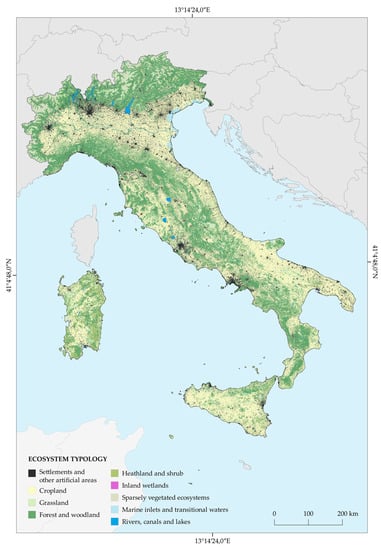
Figure 2.
Ecosystem type map with MAES compliant classification system (2018).
The spatial distribution of the ecosystem typologies of Figure 2 shows the following results (Table 4).
Table 4.
Surface statistics relating to the ecosystem typologies map for the Italian territory (2018).
From the analysis of Figure 2 and Table 4, a prevalence of the “Cropland” class emerges; it occupies more than 40% of the national territory, concentrating in Sicily, Apulia, and Emilia–Romagna, where one third of the class falls. Additionally important is the presence of the “Forest and woodland” class, which occupies approximately 30% of the national territory, with a prevalence in Tuscany, Piedmont, and Trentino–Alto Adige (more than a quarter of the surface occupied by this class falls in these three regions). The “Sparsely vegetated ecosystems” are mainly present in the alpine regions, while the “Heathland and shrub” typologies fall in the two major islands. Almost half of the coastal ecosystems are concentrated in Veneto and Friuli–Venezia Giulia, while more than 60% of those of the “Inland Wetlands” are in Tuscany, Emilia–Romagna, and Lombardy.
3.2. Assessment of Ecosystem Services through an EAGLE Compliant Land Cover Map
The 2018 land cover map used for the assessment of the two ecosystem services is shown in Figure 3.
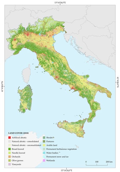
Figure 3.
Land cover map with EAGLE compliant classification system (2018).
The map refers to the EAGLE compliant classification system of Table 3, while the composition of the land cover (Figure 4) shows a prevalence of forest areas, which occupy approximately one third of the national territory (of which more than 80% consists of broad-leaved trees) and arable land, which covers 30% of the national territory. Permanent herbaceous vegetation and areas with sparse or no vegetation prevail in the high-altitude alpine areas, while olive groves and orchards occupy approximately 5% of the national territory and are particularly present in the south.
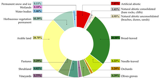
Figure 4.
Surface statistics relating to the classes of the 2018 land cover map for the Italian territory.
The assessment of ecosystem services provided the results displayed in Figure 5 for organic carbon stocks and Figure 6 for agricultural productivity, with both referring to 2018.
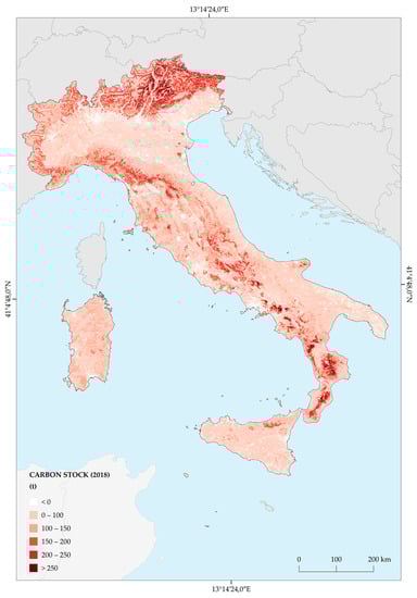
Figure 5.
Carbon stock (2018).
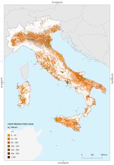
Figure 6.
Crop production (2018).
The highest carbon stock values are recorded in mountainous areas with a high presence of forest cover, in particular in the Central and Eastern Alps and in the southern Apennines. In detail, the maximum value is recorded in Trentino–Alto Adige (Figure 7), due to the significant presence of needle-leaved trees, and in Piedmont, followed by Tuscany, which is the region with the greatest extension of forest cover.
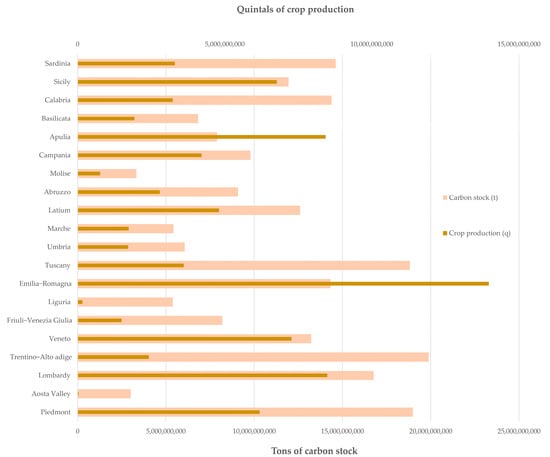
Figure 7.
National and regional values of crop production and carbon stock (2018).
Agricultural productivity varies as a function of the productivity values considered for the different territories; it shows a maximum in the Po Valley and in the hinterland of Naples (Figure 6). The maximum values are relative to Emilia–Romagna, followed by Apulia and Lombardy. Overall, productivity exceeds 10 billion quintals in 6 of the 20 regions (Figure 7).
3.3. Ecosystem Services Provided by the Types of Ecosystems
The results of the ecosystem services assessment refer to the single pixel of 10 × 10 m (Figure 5 and Figure 6). Starting with the spatialised data, the values were aggregated with respect to the types of ecosystems, allowing the results that are shown in Figure 8 and Figure 9, which respectively refer to carbon stocks and crop production by ecosystem, both for 2018.
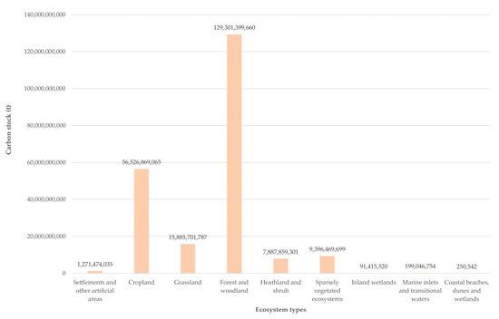
Figure 8.
Carbon stock with respect to the types of ecosystems (2018).
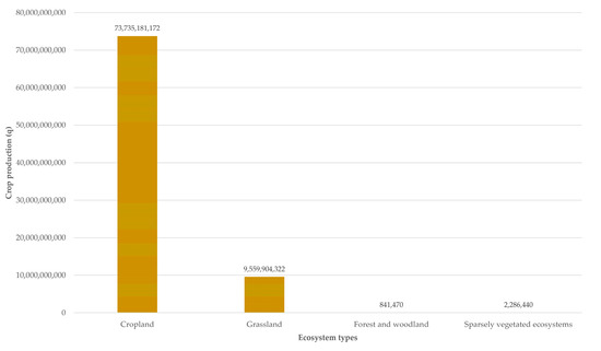
Figure 9.
Crop production with respect to the types of ecosystems (2018).
Figure 8 shows a concentration of carbon stocks in the ecosystem type of “Forest and woodland”, where 58% of the total carbon stock is concentrated, followed by “Croplands” and “Grasslands”. The remaining classes have negligible values, due to the scarce presence of vegetation.
More than 99% of the crop production is concentrated in the “Cropland” and “Grassland” classes, while marginal values can be found in “Forest and woodland” and “Sparsely vegetated ecosystems”.
4. Discussion
The approach adopted by SEEA-EA is increasingly a reference tool in the management and production of environmental data connected with the ecosystem assets and the services they provide, also allowing the analysis of the connections with economic aspects and with other human activities. In Europe, this process is rapidly evolving. Indeed, many countries have started to identify ecosystems’ extent and condition, and assess biodiversity, ecosystems, and ecosystem services at the national scale [48,49]. In some cases, these activities are aimed at improving the degree of thematic detail in ecosystem mapping, supporting the achievement of EU legislative frameworks [50,51]. The assessments require spatially explicit data and information to identify ecosystems and to delimit the LC/LU classes to be considered for the calculation of ecosystem services. Delimiting the ecosystem extent is the first of the five core accounts of SEEA-EA, with the approach defined by MAES and adopted by the UN to perform it based on a classification of the types of ecosystems according to classes derived from CLC. In recent years, several LC/LU CLMS data have been introduced based on the MAES classification system and referring to critical areas for ecosystem conservation and protection, such as Riparian Zones, Coastal Zones, and Natura 2000. This research analyses and elaborates on these data, synthesising them with the ISPRA LCM in a semantically consistent representation of the territory in terms of types of ecosystems, which can be a useful basis for conducting further studies, primarily the activity of the ecosystem extent account. The map constitutes a reference for the aggregation of the results of the physical or economic assessment of ecosystem services, informing about the relevance of each ecosystem in the provision of a given service. It also lends itself to further refinements, for example, through the introduction of geological or climatic data, or additional information for the ecosystem condition accounts, which record the condition of specific characteristics of ecosystems at specific points in time. In this sense, the map of the types of ecosystems is also suitable for conducting diachronic analysis for evaluating the changes that occurred in a given period within an ecosystem, and in its ability to provide ecosystem services or assessing trade-offs and synergies between ecosystem services [44,45,46,52,53,54]. Actually, one of the first future research developments will concern the calculation of the variation in the provision of ecosystem services associated with the LC/LU changes that occurred between 2012 and 2018, to be evaluated starting from the revised version of the ISPRA LC/LU map for 2012.
However, the map of the ecosystem typologies needs to be accompanied by more detailed spatial data for the application of estimation models for the ecosystem services physical flow account. In fact, the methodologies for calculating agricultural productivity and carbon stock described above require a detailed knowledge of the shape and composition of agricultural and natural areas, allowing also to distinguish different types of tree cover or periodic and permanent crops. The ISPRA EAGLE compliant land cover map obtained integrating CLMS data with the LCM is conceived with the aim of maximising the description of the territory from a thematic point of view, distinguishing trees from herbaceous vegetation and shrubs in mixed areas classified as “Heterogeneous agricultural areas” in the CLC and MAES input data, also considering the presence of agricultural activities or natural areas; this allows for the estimation of ecosystem services over a large area with a higher geometric detail and a better thematic characterisation of the territory compared to CLC.
The fact that the land cover map derives from the same input data used for the production of the map of the ecosystem typologies constitutes an added value for the ecosystem services accounting, since the two products are coherent from a geometric point of view and their integrated reading makes it possible to understand the composition of the land cover within a certain ecosystem or, vice versa, to deepen the ecosystem functions of the different portions of the territory pertaining to a given land cover class. In fact, comparing the two products, the map of the ecosystem typologies shows a composition of the territory in line with that found by observing the ISPRA land cover map, with a prevalence of “Cropland” in the lowland areas and of “Forest and woodland” in the alpine and Apennine areas. The shrubs are mainly on the islands, while sparse or herbaceous vegetation prevails at high altitudes. Most of the carbon stocks fall in areas classified as “Forest and woodland”, while almost all agricultural productivity falls in the “Croplands”; however, in the two ecosystems, there are not only the LC/LU classes of (respectively) trees and agricultural areas. The example of Figure 10 shows an agricultural area with a patch of natural vegetation in the central part (Figure 10a), which CLC classifies as 243 “Land principally occupied by agriculture, with significant areas of natural vegetation” (Figure 10b). By tracing the CLC class to the corresponding MAES ecosystem typology, the area falls into the “Cropland” typology (Figure 10d), while in the LC/LU map, the use of the CLC Backbone data allowed the disambiguation of the natural woody vegetation component from the agricultural component.
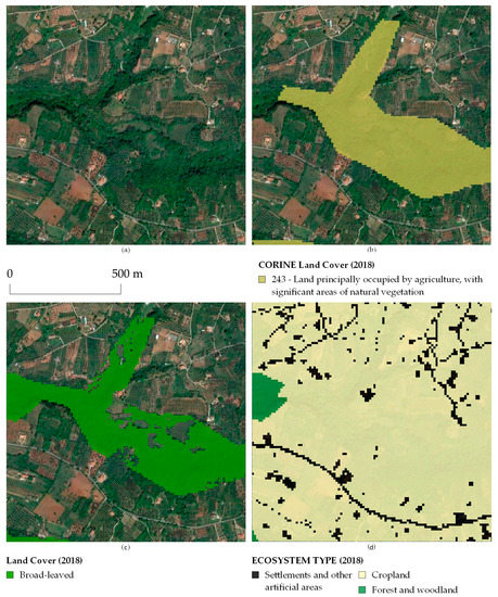
Figure 10.
Examples of land cover and land use classes within the types of ecosystems. In the example there is a patch of natural vegetation surrounded by croplands (a). The area is classified as 243 "Land mainly occupied by agriculture, with significant areas of natural vegetation" by CLC (b) and corresponds to the "Cropland" MAES ecosystem typology (d), while in the land cover map the natural woody vegetation component the from the agricultural component (c) has been disambiguated.
In this sense, the overall values of ecosystem services obtained for each ecosystem (in this case, cropland) should be understood as the synthesis of several different contributions, deriving from the presence of different classes of land cover and land use in each type of ecosystem. Figure 11 shows that the “Forest and woodland” ecosystem type also includes areas with permanent herbaceous land cover. In other cases, areas classified in the LC map as arable land or permanent crops, but also areas covered by arboreal vegetation, both broad-leaved and needle-leaved, fall into the “Cropland” typology.
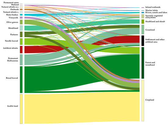
Figure 11.
Flows of land cover and land use classes within the types of ecosystems.
As in many other studies on the mapping of ecosystem types, the proposed methodology uses the CLC as reference data, trying to increase its geometric and thematic detail. Some mapping experiences conducted on a national [55] and regional [47,56] scale exploit classifications of satellite data to increase the detail of the CLC, while in other cases, the improvement is conducted on a national scale by photointerpretation with the help of ancillary data [50] or using national datasets [57,58].
In this research, to increase the detail in the description of the ecosystems, data available for the entire European territory were used (the CLMS Local data), making the methodology also applicable to medium-scale studies in other contexts, generating homogeneous and comparable data (the LCM can be replaced by Copernicus HRL Imperviousness). Furthermore, the application of the methodology is not time consuming, as it does not require significant pre-processing of the input data or intense photo-interpretation activities. The areas not covered by CLMS Local data have a lower spatial detail; however, the use of CLC Plus Backbone data still allows improvement of the description of the territory in the mixed CLC classes, disambiguating the LC classes.
5. Conclusions
This study provides insights on the integration between CLMS-derived EAGLE compliant LC/LU data and the UN approach to ecosystems classification, to supply the SEEA-EA framework for the ecosystem accounting. The five SEEA-EA core accounts integrate the main available and forthcoming data about the ecosystem assets extent, condition, and value at multiple spatial scales into a standardised, robust, and modular framework, also indicating data and knowledge gaps to be filled for a more comprehensive assessment; actually, available data often do not ensure adequate spatial and/or temporal consistency, conditioning the effectiveness of the assessment. This work focuses on ecosystem extent accounting and ecosystem services physical accounting, which require spatial LC/LU data with good thematic detail and broad coverage. The Copernicus Land Monitoring Service framework plays a fundamental role in this area, e.g., CORINE Land Cover (CLC) is one of the most suitable datasets currently used for Ecosystem accounting [24], acting as a proxy of ecosystem types for reporting purposes, although for a detailed assessment of ecosystem condition and ecosystem services physical accounting, more accurate data are needed. In this research, the CLC was integrated with the CLMS Local data and the ISPRA LCM, providing a land cover map and a map of ecosystem typologies that represent the territory in more detail and which satisfy the following requirements:
- -
- They are in line with the EAGLE (the land cover map) and MAES (the ecosystem typology map) standards in terms of classification systems;
- -
- They are comparable and compatible with each other from a geometric and thematic point of view;
- -
- They are suitable for conducting ecosystem extent accounting (the land cover map) and ecosystem services physical accounting (the type of ecosystem map).
The approach adopted by SEEA-EA is increasingly a reference tool in the management and production of environmental data connected with the ecosystem assets and the services they provide, assuming an important role in directives, reporting activities, international projects, international conventions, and platforms such as the UNCCD, Ramsar, and IPBES, and supporting the calculation and mainstreaming of Aichi indicators and SDG indicators. On the other hand, the fact that there are currently few applications of the SEEA-EA methodology [11] makes this field challenging and open to developments, especially for the definition and identification of suitable input data. This research is a first attempt to apply the SEEA-EA methodology to the Italian territory, starting from the currently available data and proposing an approach in line with the UN and EAGLE standards. On the one hand, this can be replicated in other EU territories with CLMS data availability and on the other hand, it has the potential for development, both in the integration of other SEEA-EA account activities (ecosystem condition account, monetary flow account, monetary ecosystem asset account, thematic accounts) and in the refinement of those already conducted, e.g., increasing the information content by integrating future CLC Plus products.
Author Contributions
Conceptualization, P.D.F., F.A., and M.M.; methodology, P.D.F., A.S. and A.C. (Alice Cavalli); software, P.D.F., A.S. and A.C. (Alice Cavalli); validation, P.D.F., A.S., A.C. (Alice Cavalli) and A.C. (Angela Cimini); formal analysis, P.D.F. and A.C. (Angela Cimini); investigation, P.D.F., A.S. and A.C. (Alice Cavalli); resources, M.M.; data curation, P.D.F., A.S., A.C. (Alice Cavalli) and A.C. (Angela Cimini).; writing—original draft preparation, P.D.F. and A.C. (Angela Cimini); writing—review and editing, P.D.F., A.S., A.C. (Alice Cavalli), A.C. (Angela Cimini), F.A. and D.S.; visualization, P.D.F. and A.C. (Angela Cimini); supervision, M.M. and F.A.; project administration, M.M. and F.A.; funding acquisition, M.M. and F.A. All authors have read and agreed to the published version of the manuscript.
Funding
This research was funded by the Italian Institute for Environmental Protection and Research (ISPRA) structural funds.
Data Availability Statement
Data presented in this study are available on request from the corresponding author. The data are not publicly available because they are part of ongoing research.
Conflicts of Interest
The authors declare no conflict of interest.
References
- Simon, F.; Karachepone, N.N.; Paul, L.; Rob, A. The Methodological Assessment Report on Scenarios and Models of Biodiversity and Ecosystem Services; Secretariat of the Intergovernmental Science-Policy Platform on Biodiversity and Ecosystem Services: Bonn, Germany, 2016; pp. 1–348. [Google Scholar]
- Joachim, M.; Anne, T.; Markus, E.; Bruna, G.; José, I.B.; Maria Luisa, P.; Sophie, C.; Francesca, S.; Alberto, O.; Arwyn, J.; et al. Mapping and Assessment of Ecosystems and Their Services. An Analytical Framework for Mapping and Assessment of Ecosystem Condition in EU; European Union: Luxembourg, 2018. [Google Scholar]
- Vargas, L.; Willemen, L.; Hein, L. Assessing the Capacity of Ecosystems to Supply Ecosystem Services Using Remote Sensing and An Ecosystem Accounting Approach. Environ. Manage. 2019, 63, 1–15. [Google Scholar] [CrossRef] [PubMed]
- Bailey, R.G. Ecoregions of the United States. In Ecosystem Geography; Springer: Berlin/Heidelberg, Germany, 1996; pp. 83–104. [Google Scholar]
- Dale, V.H.; Brown, S.; Haeuber, R.A.; Hobbs, N.T.; Huntly, N.; Naiman, R.J.; Riebsame, W.E.; Turner, M.G.; Valone, T.J. Ecological Principles and Guidelines for Managing the Use of Land Sup> 1. Ecol. Appl. 2000, 10, 639–670. [Google Scholar]
- Keith, D.A.; Rodríguez, J.P.; Brooks, T.M.; Burgman, M.A.; Barrow, E.G.; Bland, L.; Comer, P.J.; Franklin, J.; Link, J.; McCarthy, M.A. The IUCN Red List of Ecosystems: Motivations, Challenges, and Applications. Conserv. Lett. 2015, 8, 214–226. [Google Scholar] [CrossRef]
- Keith, D.A.; Ferrer-Paris, J.R.; Nicholson, E.; Bishop, M.J.; Polidoro, B.A.; Ramirez-Llodra, E.; Tozer, M.G.; Nel, J.L.; Mac Nally, R.; Gregr, E.J.; et al. A Function-Based Typology for Earth’s Ecosystems. Nature 2022, 610, 513–518. [Google Scholar] [CrossRef]
- European Commission. EU Biodiversity Strategy for 2030. Bringing Nature Back into Our Lives; European Commission: Brussels, Belgium, 2020. [Google Scholar]
- European Commission. EU Soil Strategy for 2030. Reaping the Benefits of Healthy Soils for People, Food, Nature and Climate; European Commission: Brussels, Belgium, 2021. [Google Scholar]
- European Commission. Regulation of the European Parliament and of the Council on Nature Restoration; European Commission: Brussels, Belgium, 2022. [Google Scholar]
- Vallecillo, S.; Maes, J.; Teller, A.; Babí Almenar, J.; Barredo, J.I.; Trombetti, M.; Malak, A. EU-Wide Methodology to Map and Assess Ecosystem Condition. Towards a Common Approach Consistent with a Global Statistical Standard; European Commission: Brussels, Belgium, 2022; ISBN 9789276570295. [Google Scholar]
- European Union. Establishing a Framework for Community Action in the Field of Marine Environmental Policy (Marine Strategy Framework Directive); European Commission: Brussels, Belgium, 2008. [Google Scholar]
- European Commission. Establishing Rules on Support for Strategic Plans to Be Drawn up by Member States under the Common Agricultural Policy (CAP Strategic Plans) and Financed by the European Agricultural Guarantee Fund (EAGF) and by the European Agricultural Fund for Rural Development (EAFRD) and Repealing Regulation (EU) No1305/2013 of the European Parliament and of the Council and Regulation (EU) No 1307/2013 of the European Parliament and of the Council; European Commission: Brussels, Belgium, 2018. [Google Scholar]
- European Commission. A New EU Forest Strategy: For Forests and the Forest-Based Sector; European Commission: Brussels, Belgium, 2013. [Google Scholar]
- European Commission. EU Pollinators Initiative; European Commission: Brussels, Belgium, 2018. [Google Scholar]
- van Egmond, F.M. Towards Climate-Smart Sustainable Management of Agricultural Soils. Deliverable 6.1. Report on Harmonized Procedures for Creation of Databases and Maps. Available online: https://ejpsoil.eu/fileadmin/projects/ejpsoil/WP6/EJP_SOIL_D6.1_Report_on_harmonized_procedures_for_creation_of_databases_and_maps_revised_vf__1_.pdf (accessed on 10 October 2022).
- United Nations. Transforming Our World: The 2030 Agenda for Sustainable Development; United Nations: New York, NY, USA, 2015. [Google Scholar]
- UNSD. Using the SEEA EA for Calculating Selected SDG Indicators. Report of the NCAVES Project; UNSD: New York, NY, USA, 2020. [Google Scholar]
- UN Cover Note for Area A: Coordination, Discussion on UN Sustainable Development Goals (SDGs). Available online: https://seea.un.org/sites/seea.un.org/files/sdg_cover_note_broadbrush.pdf (accessed on 3 November 2022).
- Secretariat of the Convention on Biological Diversity; UN Environment; UN Statistics Division. SDG Indicator 15.9.1 Metadata. Available online: https://unstats.un.org/sdgs/metadata/files/Metadata-15-09-01.pdf (accessed on 3 November 2022).
- United Nations Committee of Experts on Environmental-Economic Accounting. System of Environmental Economic Accounting 2012: Experimental Ecosystem Accounting 2012; UNCEEA: New York, NY, USA, 2014; ISBN 9789211615753. [Google Scholar]
- UN-Department of economic and social affairs System of Environmental-Economic Accounting-Ecosystem Accounting: Final Draft; UN DESA: New York, NY, USA, 2021.
- Edens, B.; Maes, J.; Hein, L.; Obst, C.; Siikamaki, J.; Schenau, S.; Javorsek, M.; Chow, J.; Chan, J.Y.; Steurer, A.; et al. Establishing the SEEA Ecosystem Accounting as a Global Standard. Ecosyst. Serv. 2022, 54, 101413. [Google Scholar] [CrossRef]
- European Commission. Directorate-General for the Environment. Mapping and Assessment of Ecosystems and Their Services: An Analytical Framework for Ecosystem Assessments under Action 5 of the EU Biodiversity Strategy to 2020: Discussion Paper—Final, April 2013; European Commission: Brussels, Belgium, 2013; ISBN 9789279293696. [Google Scholar]
- Veronika, V.; Joachim, M.; Jan-Erik, P.; Alessandra, L.N.; Sara, V.; Nerea, A.; Eva, I.; Anne, T. Accounting for Ecosystems and Their Services in the European Union (INCA). Final Report from Phase II of the INCA Project Aiming to Develop a Pilot for an Integrated System of Ecosystem Accounts for the EU; Publications office of the European Union: Luxembourg, 2021. [Google Scholar]
- European Environmental Agency. Riparian Zones Nomenclature Guideline 2021; European Environmental Agency: Copenhagen, Denmark, 2021. [Google Scholar]
- European Environmental Agency. Copernicus Land Monitoring Service-Local Component: Coastal Zones Monitoring Nomenclature Guideline 2021; European Environmental Agency: Copenhagen, Denmark, 2021. [Google Scholar]
- Buck, O.; Sousa, A. Copernicus Land Monitoring Service N2K User Manual (Version 1.0); European Environmental Agency: Copenhagen, Denmark, 2021. [Google Scholar]
- Büttner, G.; Kosztra, B.; Maucha, G.; Pataki, R.; Kleeschulte, S.; Hazeu, G.; Vittek, M.; Littkopf, A. Copernicus Land Monitoring Service CORINE Land Cover Product User Manual (Version 1.0); Environmental Agency: Copenhagen, Denmark, 2021.
- European Commission. Mapping Guide v6.2 for a European Urban Atlas Regional Policy; European Commission: Brussels, Belgium, 2020. [Google Scholar]
- Kleeschulte, S.; Banko, G.; Smith, G.; Arnold, S.; Scholz, J.; Kosztra, B.; Maucha, G. Refined Details on CLC+ Backbone Specifications, Criteria for CLC+. Available online: https://land.copernicus.eu/user-corner/technical-library/clc-core-consultations-for-the-technical-specifications (accessed on 3 November 2022).
- Arnold, S.; Kosztra, B.; Banko, G.; Milenov, P.; Smith, G.; Hazeu, G.; Bock, M.; Perger, C.; Caetano, M. Explanatory Documentation of the EAGLE Concept-Version 3.1.2; European Environmental Agency: Copenhagen, Denmark, 2021. [Google Scholar]
- De Fioravante, P.; Luti, T.; Cavalli, A.; Giuliani, C.; Dichicco, P.; Marchetti, M.; Chirici, G.; Congedo, L.; Munafò, M. Multispectral Sentinel-2 and Sar Sentinel-1 Integration for Automatic Land Cover Classification. Land 2021, 10, 611. [Google Scholar] [CrossRef]
- Spadoni, G.L.; Cavalli, A.; Congedo, L.; Munafò, M. Analysis of Normalized Difference Vegetation Index (NDVI) Multi-Temporal Series for the Production of Forest Cartography. Remote Sens. Appl. Soc. Environ. 2020, 20, 100419. [Google Scholar] [CrossRef]
- Luti, T.; De Fioravante, P.; Marinosci, I.; Strollo, A.; Riitano, N.; Falanga, V.; Mariani, L.; Congedo, L.; Munafò, M. Land Consumption Monitoring with SAR Data and Multispectral Indices. Remote Sens. 2021, 13, 1586. [Google Scholar] [CrossRef]
- De Fioravante, P.; Strollo, A.; Assennato, F.; Marinosci, I.; Congedo, L.; Munafò, M. High Resolution Land Cover Integrating Copernicus Products: A 2012–2020 Map of Italy. Land 2022, 11, 35. [Google Scholar] [CrossRef]
- Michele, M. Consumo Di Suolo, Dinamiche Territoriali e Servizi Ecosistemici; Report SNPA, 32/22; Istituto superiore per la protezione e la ricerca ambientale: Roma, Italy, 2022. [Google Scholar]
- Haines-Young, R.; Potschin, M. Common International Classification of Ecosystem Services (CICES) V5.1 Guidance on the Application of the Revised Structure; Fabis Consulting Ltd.: Nottingham, UK, 2018. [Google Scholar]
- Assennato, F.; Smiraglia, D.; Cavalli, A.; Congedo, L.; Giuliani, C.; Riitano, N.; Strollo, A.; Munafò, M. The Impact of Urbanization on Land: A Biophysical-Based Assessment of Ecosystem Services Loss Supported by Remote Sensed Indicators. Land 2022, 11, 236. [Google Scholar] [CrossRef]
- ISTAT 6° Censimento Generale Dell’Agricoltura. Available online: https://www.istat.it/it/files//2014/03/Atlante-dellagricoltura-italiana.-6°-Censimento-generale-dellagricoltura.pdf (accessed on 20 October 2022).
- Hutyra, L.R.; Yoon, B.; Alberti, M. Terrestrial Carbon Stocks across a Gradient of Urbanization: A Study of the Seattle, WA Region. Glob. Chang. Biol. 2011, 17, 783–797. [Google Scholar] [CrossRef]
- Li, S.; Liu, Y.; Yang, H.; Yu, X.; Zhang, Y.; Wang, C. Integrating Ecosystem Services Modeling into Effectiveness Assessment of National Protected Areas in a Typical Arid Region in China. J. Environ. Manage. 2021, 297, 113408. [Google Scholar] [CrossRef] [PubMed]
- Penman, J.; Gytarsky, M.; Hiraishi, T.; Krug, T.; Kruger, D.; Pipatti, R.; Buendia, L.; Miwa, K.; Ngara, T.; Tanabe, K. Good Practice Guidance for Land Use, Land-Use Change and Forestry; Institute for Global Environmental Strategies: Kanagawa, Japan, 2003. [Google Scholar]
- Obiang Ndong, G.; Therond, O.; Cousin, I. Analysis of Relationships between Ecosystem Services: A Generic Classification and Review of the Literature. Ecosyst. Serv. 2020, 43, 101120. [Google Scholar] [CrossRef]
- Saidi, N.; Spray, C. Ecosystem Services Bundles: Challenges and Opportunities for Implementation and Further Research. Environ. Res. Lett. 2018, 13, 113001. [Google Scholar] [CrossRef]
- Renard, D.; Rhemtulla, J.M.; Bennett, E.M. Historical Dynamics in Ecosystem Service Bundles. Proc. Natl. Acad. Sci. USA 2015, 112, 13411–13416. [Google Scholar] [CrossRef]
- Farrell, C.A.; Coleman, L.; Kelly-Quinn, M.; Obst, C.G.; Eigenraam, M.; Norton, D.; O’donoghue, C.; Kinsella, S.; Delargy, O.; Stout, J.C. Applying the System of Environmental Economic Accounting-Ecosystem Accounting (Seea-Ea) Framework at Catchment Scale to Develop Ecosystem Extent and Condition Accounts. One Ecosyst. 2021, 6, e65582. [Google Scholar] [CrossRef]
- Schröter, M.; Albert, C.; Marques, A.; Tobon, W.; Lavorel, S.; Maes, J.; Brown, C.; Klotz, S.; Bonn, A. National Ecosystem Assessments in Europe: A Review. Bioscience 2016, 66, 813–828. [Google Scholar] [CrossRef]
- Alessandra, L.N.; Ioanna, G.; Karsten, G.; David, B.; Beyhan, E. Ecosystem and Ecosystem Services Accounts: Time for Applications; Publications Office of the European Union: Luxembourg, 2021. [Google Scholar]
- Blasi, C.; Capotorti, G.; Alós Ortí, M.M.; Anzellotti, I.; Attorre, F.; Azzella, M.M.; Carli, E.; Copiz, R.; Garfì, V.; Manes, F.; et al. Ecosystem Mapping for the Implementation of the European Biodiversity Strategy at the National Level: The Case of Italy. Environ. Sci. Policy 2017, 78, 173–184. [Google Scholar] [CrossRef]
- Laporta, L.; Domingos, T.; Marta-Pedroso, C. Mapping and Assessment of Ecosystems Services under the Proposed Maes European Common Framework: Methodological Challenges and Opportunities. Land 2021, 10, 1040. [Google Scholar] [CrossRef]
- Vallet, A.; Locatelli, B.; Levrel, H.; Wunder, S.; Seppelt, R.; Scholes, R.J.; Oszwald, J. Relationships Between Ecosystem Services: Comparing Methods for Assessing Tradeoffs and Synergies. Ecol. Econ. 2018, 150, 96–106. [Google Scholar] [CrossRef]
- Zhang, Z.; Liu, Y.; Wang, Y.; Liu, Y.; Zhang, Y.; Zhang, Y. What Factors Affect the Synergy and Tradeoff between Ecosystem Services, and How, from a Geospatial Perspective? J. Clean. Prod. 2020, 257, 120454. [Google Scholar] [CrossRef]
- Raudsepp-Hearne, C.; Peterson, G.D.; Bennett, E.M. Ecosystem Service Bundles for Analyzing Tradeoffs in Diverse Landscapes. Proc. Natl. Acad. Sci. USA 2010, 107, 5242–5247. [Google Scholar] [CrossRef] [PubMed]
- Grunewald, K.; Schweppe-Kraft, B.; Syrbe, R.U.; Meier, S.; Krüger, T.; Schorcht, M.; Walz, U. Hierarchical Classification System of Germany’s Ecosystems as Basis for an Ecosystem Accounting—Methods and First Results. One Ecosyst. 2020, 5, e50648. [Google Scholar] [CrossRef]
- Sieber, I.M.; Hinsch, M.; Vergílio, M.; Gil, A.; Burkhard, B. Assessing the Effects of Different Land-Use/Landcover Input Datasets on Modelling and Mapping Terrestrial Ecosystem Services—Case Study Terceira Island (Azores, Portugal). One Ecosyst. 2021, 6, e69119. [Google Scholar] [CrossRef]
- Černecký, J.; Gajdoš, P.; Špulerová, J.; Halada, Ľ.; Mederly, P.; Ulrych, L.; Ďuricová, V.; Švajda, J.; Černecká, Ľ.; Andráš, P.; et al. Ecosystems in Slovakia. J. Maps 2020, 16, 28–35. [Google Scholar] [CrossRef]
- Vačkář, D.; Grammatikopoulou, I.; Danĕk, J.; Krkoška Lorencová, E. Methodological Aspects of Ecosystem Service Valuation at the National Level. One Ecosyst. 2018, 3, e25508. [Google Scholar] [CrossRef]


Disclaimer/Publisher’s Note: The statements, opinions and data contained in all publications are solely those of the individual author(s) and contributor(s) and not of MDPI and/or the editor(s). MDPI and/or the editor(s) disclaim responsibility for any injury to people or property resulting from any ideas, methods, instructions or products referred to in the content. |
© 2023 by the authors. Licensee MDPI, Basel, Switzerland. This article is an open access article distributed under the terms and conditions of the Creative Commons Attribution (CC BY) license (https://creativecommons.org/licenses/by/4.0/).